Annealed and quenched representations of the Gauss-Rényi measure by “periodic points”

Shintaro Suzuki and Hiroki Takahasi Department of Mathematics, Tokyo Gakugei University, 4-1-1 Nukuikita-machi Koganei-shi, Tokyo, 184-8501, JAPAN shin05@u-gakugei.ac.jp Keio Institute of Pure and Applied Sciences (KiPAS), Department of Mathematics, Keio University, Yokohama, 223-8522, JAPAN hiroki@math.keio.ac.jp

Abstract.

We consider independently identically distributed random compositions of the Gauss and Rényi maps that generate random continued fractions. Using methods of ergodic theory, thermodynamic formalism and large deviations, we show that weighted cycles of this random dynamical system equidistribute with respect to the Gauss-Rényi measure. We present both annealed (sample-averaged) and quenched (samplewise) results.

2020 Mathematics Subject Classification:

11K50, 37A40, 37A44, 37C40

Keywords: random dynamical system; periodic points; the Gauss map; the Rényi map

1. Introduction

One leading idea in the qualitative theory of deterministic dynamical systems is to use the collection of periodic orbits as a spine to structure the dynamics. This idea traces back to Poincaré [32]: “… ce qui nous rend ces solutions périodiques si précieuses, … la seul brèche par où nous puissions esseyer de pénétrer dans une place jusqu’ici réputée inabordable.” Bowen’s pioneering results [7, 8] assert that periodic points of topologically mixing Axiom A diffeomorphisms equidistribute with respect to the measure of maximal entropy. The importance of periodic orbits in descriptions of ergodic properties of natural invariant probability measures has long been recognized in the physics literature, see e.g., [10, 17]. Cvitanović [10] proposed expansions of dynamical characteristics into series or products that consist of infinitely many periodic orbits, to better analyze the characteristics taking advantage of the simple structure of each periodic orbit in the expansions.

By deterministic dynamical systems, we mean ordinary differential equations or iterated maps. Systems with multiple evolution laws, called random dynamical systems [5], are also relevant to consider. For a large class of random dynamical systems, we expect that periodic orbits still play significant roles, but it is not clear how periodic points should be defined.

In discrete time, deterministic dynamical systems are iterations of one fixed map, whereas random dynamical systems are compositions of different maps chosen at random. A naive idea is to use fixed points of random compositions of $n$ maps as substitutes for periodic points of period $n$ . Such “periodic points” have been indeed considered, see e.g., [9, 33, 37]. For other substitutes for the concept of periodic points in the context random dynamical systems, see e.g., [13, 21, 25].

In [37], the authors proved an analogue of Bowen’s equidistribution theorem [7, 8] for random dynamical systems generated by a class of interval maps with finitely many branches. The aim of this paper is to extend this analogue to random dynamical systems generated by the Gauss and Rényi maps. The Gauss map $T_{0}\colon(0,1]\to[0,1)$ and the Rényi map $T_{1}\colon[0,1)\to[0,1)$ are respectively given by

T_{0}x=\frac{1}{x}-\left\lfloor\frac{1}{x}\right\rfloor\quad\text{and}\quad T_{1}x=\frac{1}{1-x}-\left\lfloor\frac{1}{1-x}\right\rfloor.

The graph of $T_{1}$ is obtained by reversing the graph of $T_{0}$ around the axis $\{x=1/2\}$ , as shown in Figure 1. Since both maps have infinitely many branches, the random dynamical systems they generate are beyond the scope of [37].

Refer to caption — Figure 1. The graph of the Gauss map $T_{0}$ (left) and that of the Rényi map $T_{1}$ (right): $T_{0}^{-1}(0)=\{1/k\colon k\in\mathbb{N}\}$ , $T_{1}^{-1}(0)=\{(k-1)/k\colon k\in\mathbb{N}\}$ ; $T_{0}^{-1}(1)=T_{1}^{-1}(1)=\emptyset$ ; $T_{1}0=0$ , $T_{1}^{\prime}0=1$ .

For a sample path $\omega=(\omega_{n})_{n=1}^{\infty}$ in the product space $\Omega=\{0,1\}^{\mathbb{N}}$ of the discrete space $\{0,1\}$ , we consider a random composition

T_{\omega}^{n}=T_{\omega_{n}}\circ T_{\omega_{n-1}}\circ\cdots\circ T_{\omega_{1}}\ \text{ for }n\in\mathbb{N}.

Write $T_{\omega}^{0}$ for the identity map on $[0,1]$ . Let $\Lambda_{\omega}$ denote the set of $x\in[0,1]$ such that $T_{\omega}^{n}x$ is defined for every $n\in\mathbb{N}$ . Each $x\in\Lambda_{\omega}$ has a continued fraction expansion

(1.1)

x=\omega_{1}+\frac{\displaystyle{\hfill{(-1)^{\omega_{1}}}\hfill\;\vrule}}{\displaystyle{\vrule\;\hfill{C_{1}(\omega,x)}\hfill}}+\frac{\displaystyle{\hfill{(-1)^{\omega_{2}}}\hfill\;\vrule}}{\displaystyle{\vrule\;\hfill{C_{2}(\omega,x)}\hfill}}+\frac{\displaystyle{\hfill{(-1)^{\omega_{3}}}\hfill\;\vrule}}{\displaystyle{\vrule\;\hfill{C_{3}(\omega,x)}\hfill}}+\cdots,

where each $C_{n}(\omega,x)$ , $n\in\mathbb{N}$ is a positive integer that is determined by $T_{\omega}^{n-1}x$ , $\omega_{n}$ , $\omega_{n+1}$ , and satisfies $(-1)^{\omega_{n+1}}+C_{n}(\omega,x)\geq 1$ (see $\S$ 2.1 for details). This type of continued fractions was first considered by Perron [29]. In the case $\omega_{n}=0$ for all $n\in\mathbb{N}$ we obtain the well-known regular continued fraction

x=\frac{\displaystyle{\hfill{1}\hfill\;\vrule}}{\displaystyle{\vrule\;\hfill{A_{1}(x)}\hfill}}+\frac{\displaystyle{\hfill{1}\hfill\;\vrule}}{\displaystyle{\vrule\;\hfill{A_{2}(x)}\hfill}}+\frac{\displaystyle{\hfill{1}\hfill\;\vrule}}{\displaystyle{\vrule\;\hfill{A_{3}(x)}\hfill}}+\cdots,

where $A_{n}(x)=\lfloor 1/T_{0}^{n-1}x\rfloor$ for $n\in\mathbb{N}$ . In the case $\omega_{n}=1$ for all $n\in\mathbb{N}$ we obtain the backward continued fraction

x=1-\frac{\displaystyle{\hfill{1}\hfill\;\vrule}}{\displaystyle{\vrule\;\hfill{B_{1}(x)}\hfill}}-\frac{\displaystyle{\hfill{1}\hfill\;\vrule}}{\displaystyle{\vrule\;\hfill{B_{2}(x)}\hfill}}-\frac{\displaystyle{\hfill{1}\hfill\;\vrule}}{\displaystyle{\vrule\;\hfill{B_{3}(x)}\hfill}}-\cdots,

where $B_{n}(x)=\lfloor 1/(1-T_{1}^{n-1}x)\rfloor+1$ for $n\in\mathbb{N}$ . The backward continued fraction was used, for example, in computing certain inhomogeneous approximation constants [31]. For its connection with geodesic flows, see [3].

It is the essential difference between statistical properties of the sequences $(A_{n}(x))_{n=1}^{\infty}$ and $(B_{n}(x))_{n=1}^{\infty}$ that makes the random continued fraction interesting. For Lebesgue almost every irrational $x$ in $(0,1)$ , each positive integer $k$ appears in $(A_{n}(x))_{n=1}^{\infty}$ with frequency $\frac{1}{\log 2}\log\frac{(k+1)^{2}}{k(k+2)}$ , while the frequency of $2$ in $(B_{n}(x))_{n=1}^{\infty}$ is $1$ . This is due to the fact that $T_{0}$ leaves invariant the Gauss measure $d\lambda_{0}=\frac{1}{\log 2}\frac{dx}{x+1}$ , while $T_{1}$ leaves invariant the infinite measure $\frac{dx}{x}$ . More precisely, $x=0$ is a neutral fixed point of $T_{1}$ : $T_{1}0=0$ and $T_{1}^{\prime}0=1$ . For more comparisons of the regular and backward continued fractions as well as more information on the singular behavior of the digit sequence in the backward continued fraction, see [1, 2, 19, 38, 42] for example.

1.1. Statements of results

We consider an independently identically distributed (i.i.d.) random dynamical system generated by $T_{0}$ and $T_{1}$ . This means that $T_{1}$ is chosen with a fixed probability $p\in(0,1)$ at each step. Let $m_{p}$ denote the Bernoulli measure on the sample space $\Omega$ associated with the probability vector $(1-p,p)$ . By [18, Theorem 5.2], there exists a unique Borel probability measure $\lambda_{p}$ on $[0,1]$ that is absolutely continuous with respect to the Lebesgue measure on $[0,1]$ and satisfies $\mu=(1-p)\cdot\mu\circ T_{0}^{-1}+p\cdot\mu\circ T_{1}^{-1}$ . The measure $\lambda_{p}$ , called the Gauss-Rényi measure, is significant since for $m_{p}$ -almost every $\omega\in\Omega$ and Lebesgue almost every $x\in\Lambda_{\omega}$ , we have

\lim_{n\to\infty}\frac{1}{n}\sum_{i=0}^{n-1}f(T_{\omega}^{i}x)=\int fd\lambda_{p}\ \text{ for any continuous $f\colon[0,1]\to\mathbb{R}$.}

For $p\in[0,1)$ , let $h_{p}\colon[0,1]\to[0,\infty)$ denote the Radon-Nikodým derivative of $\lambda_{p}$ with respect to the Lebesgue measure on $[0,1]$ . We know that $h_{0}(x)=\frac{1}{\log 2}\frac{1}{x+1}$ . For any $p\in(0,1)$ , $h_{p}$ is bounded from above and away from $0$ [23, Proposition 3.4]. An explicit formula for $h_{p}$ is desired, since it is related to the frequency of digits in the random continued fraction expansion (2.1). Up to present, no algebraic formula for $h_{p}$ is known except for the case $p=0$ . Kalle et al. proved that $h_{p}$ is $C^{\infty}$ for any $p\in(0,1)$ [24]. Bousoun et al. [6] obtained a functional-analytic formula for $h_{p}$ for $p\in(0,1)$ sufficiently near $0$ .

Our aim here is to represent $\lambda_{p}$ and $h_{p}$ for any $p\in(0,1)$ , using the collection of “periodic points”

\bigcup_{\omega\in\Omega}\bigcup_{n=1}^{\infty}{\rm Fix}(T_{\omega}^{n}),\ \ {\rm Fix}(T_{\omega}^{n})=\{x\in\Lambda_{\omega}\colon T_{\omega}^{n}x=x\}.

Elements of this set are called random cycles [37]. We first present a quenched (samplewise) representation, and then an annealed (sample-averaged) one. For $\omega\in\Omega$ and $n\in\mathbb{N}$ define

(1.2)

Z_{\omega,n}=\sum_{x\in{\rm Fix}(T_{\omega}^{n})}\!\!\!\!\!\!|(T_{\omega}^{n})^{\prime}x|^{-1},

which plays the role of a normalizing constant. The derivatives of $T_{0}$ and $T_{1}$ at their discontinuities are the one-sided derivatives. For a topological space $X$ , let $\mathcal{M}(X)$ denote the space of Borel probability measures on $X$ endowed with the weak* topology. For $\omega\in\Omega$ , $x\in\Lambda_{\omega}$ and $n\in\mathbb{N}$ , let $V_{n}^{\omega}(x)\in\mathcal{M}([0,1])$ denote the uniform probability distribution on the random orbit $(T_{\omega}^{i}x)_{i=0}^{n-1}$ . For $p\in\{0,1\}$ , let $m_{p}$ denote the Borel probability measure on $\Omega$ that is the unit point mass at the point $p^{\infty}=ppp\cdots$ in $\Omega$ . Let $\lambda_{1}\in\mathcal{M}([0,1])$ denote the unit point mass at $0$ .

Theorem 1.1 (quenched representation of the Gauss-Rényi measure).

Let $p\in(0,1)$ . The following statements hold:

(a)

for $m_{p}$ -almost every $\omega\in\Omega$ and any continuous function $F\colon\mathcal{M}([0,1])\to\mathbb{R}$ ,

\lim_{n\to\infty}\frac{1}{Z_{\omega,n}}\sum_{x\in{\rm Fix}(T_{\omega}^{n})}|(T^{n}_{\omega})^{\prime}x|^{-1}F(V_{n}^{\omega}(x))=F(\lambda_{p});

(b)

for $m_{p}$ -almost every $\omega\in\Omega$ and any continuous function $f\colon[0,1]\to\mathbb{R}$ ,

\lim_{n\to\infty}\frac{1}{Z_{\omega,n}}\sum_{x\in{\rm Fix}(T^{n}_{\omega})}|(T_{\omega}^{n})^{\prime}x|^{-1}\int fdV_{n}^{\omega}(x)=\int fd\lambda_{p}.

As already noted, the cases $p=0$ and $p=1$ correspond to the iteration of $T_{0}$ and that of $T_{1}$ respectively. The convergences in Theorem 1.1 in these two cases were established in [40] (see [15] for a closely related result) and [42] respectively. The main concern of this paper is the case $p\in(0,1)$ .

Theorem 1.1(a) implies Theorem 1.1(b) (see §2.4). The latter deserves to be called a quenched representation of $\lambda_{p}$ in terms of random cycles. For $\omega\in\Omega$ , $x\in\Lambda_{\omega}$ , a subset $A$ of $[0,1]$ and $n\in\mathbb{N}$ , let

e_{n}(\omega,x,A)=\frac{\#\{0\leq i\leq n-1\colon T_{\omega}^{i}x\in A\}}{n}.

By the portmanteau theorem, Theorem 1.1(b) is equivalent to the following: for $m_{p}$ -almost every $\omega\in\Omega$ and any Borel subset $A$ of $[0,1]$ with $\lambda_{p}(\partial A)=0$ ,

(1.3)

\lim_{n\to\infty}\frac{1}{Z_{\omega,n}}\sum_{x\in{\rm Fix}(T^{n}_{\omega})}|(T_{\omega}^{n})^{\prime}x|^{-1}e_{n}(\omega,x,A)=\lambda_{p}(A).

The meaning of Theorem 1.1(a) may be a little less intuitive Theorem 1.1(b). By the portmanteau theorem it is equivalent to the following: for for $m_{p}$ -almost every $\omega\in\Omega$ and any Borel subset $\mathcal{A}$ of $\mathcal{M}(\Lambda)$ with $\lambda_{p}\notin\partial\mathcal{A}$ ,

\lim_{n\to\infty}\frac{1}{Z_{\omega,n}}\sum_{\begin{subarray}{c}x\in{\rm Fix}(T_{\omega}^{n})\\ V_{n}^{\omega}(x)\in\mathcal{A}\end{subarray}}|(T^{n}_{\omega})^{\prime}x|^{-1}=\mbox{1}\hskip-2.5pt\mbox{l}_{\mathcal{A}}(\lambda_{p}),

where $\mbox{1}\hskip-2.5pt\mbox{l}_{\mathcal{A}}$ denotes the indicator function of $\mathcal{A}$ . In particular, if $\lambda_{p}\in\mathcal{A}$ then $V_{n}^{\omega}(x)\in\mathcal{A}$ holds for almost every $x\in{\rm Fix}(T_{\omega}^{n})$ as $n\to\infty$ .

To move on to an annealed counterpart, for $p\in[0,1]$ , $n\in\mathbb{N}$ and $\omega\in\Omega$ we set

Z_{p,n}=\int Z_{\omega,n}dm_{p}(\omega),

which plays the role of a normalizing constant.

Theorem 1.2 (annealed representation of the Gauss-Rényi measure).

Let $p\in(0,1)$ . The following statements hold:

(a)

for any continuous function $F\colon\mathcal{M}([0,1])\to\mathbb{R}$ ,

\lim_{n\to\infty}\frac{1}{Z_{p,n}}\int dm_{p}(\omega)\sum_{x\in{\rm Fix}(T_{\omega}^{n})}|(T_{\omega}^{n})^{\prime}x|^{-1}F(V_{n}^{\omega}(x))=F(\lambda_{p});

(b)

for any continuous function $f\colon[0,1]\to\mathbb{R}$ ,

\lim_{n\to\infty}\frac{1}{Z_{p,n}}\int dm_{p}(\omega)\sum_{x\in{\rm Fix}(T_{\omega}^{n})}|(T_{\omega}^{n})^{\prime}x|^{-1}\int fdV^{\omega}_{n}(x)=\int fd\lambda_{p}.

Theorem 1.2(a) implies Theorem 1.2(b) (see §2.3). The latter deserves to be called an annealed representation of $\lambda_{p}$ in terms of random cycles since it is equivalent to the following: for any Borel subset $A$ of $[0,1]$ with $\lambda_{p}(\partial A)=0$ ,

(1.4)

\lim_{n\to\infty}\frac{1}{Z_{p,n}}\int dm_{p}(\omega)\sum_{x\in{\rm Fix}(T^{n}_{\omega})}|(T_{\omega}^{n})^{\prime}x|^{-1}e_{n}(\omega,x,A)=\lambda_{p}(A).

Theorem 1.2(a) is equivalent to the following: for any Borel subset $\mathcal{A}$ of $\mathcal{M}(\Lambda)$ with $\lambda_{p}\notin\partial\mathcal{A}$ ,

\lim_{n\to\infty}\frac{1}{Z_{p,n}}\int dm_{p}(\omega)\sum_{\begin{subarray}{c}x\in{\rm Fix}(T_{\omega}^{n})\\ V_{n}^{\omega}(x)\in\mathcal{A}\end{subarray}}|(T^{n}_{\omega})^{\prime}x|^{-1}=\mbox{1}\hskip-2.5pt\mbox{l}_{\mathcal{A}}(\lambda_{p}).

Since the Radon-Nikodým derivative $h_{p}$ of the Gauss-Rényi measure $\lambda_{p}$ is continuous, from (1.3) and (1.4) we obtain its quenched and annealed representations in terms of random cycles.

Corollary 1.3 (quenched and annealed representations of the Radon-Nikodým derivative).

Let $p\in(0,1)$ . The following statements hold:

(a)

for $m_{p}$ -almost every $\omega\in\Omega$ and any $y\in(0,1)$ ,

h_{p}(y)=\lim_{\varepsilon\to+0}\frac{1}{2\varepsilon}\lim_{n\to\infty}\frac{1}{Z_{\omega,n}}\sum_{x\in{\rm Fix}(T^{n}_{\omega})}|(T_{\omega}^{n})^{\prime}x|^{-1}e_{n}(\omega,x,[y-\varepsilon,y+\varepsilon]);

(b)

for any $y\in(0,1)$ ,

h_{p}(y)=\lim_{\varepsilon\to+0}\frac{1}{2\varepsilon}\lim_{n\to\infty}\frac{1}{Z_{p,n}}\int dm_{p}(\omega)\sum_{x\in{\rm Fix}(T_{\omega}^{n})}|(T_{\omega}^{n})^{\prime}x|^{-1}e_{n}(\omega,x,[y-\varepsilon,y+\varepsilon]).

Our main results altogether assert that the collection of random cycles capture relevant information of the Gauss-Rényi random dynamics. Since random cycles can be defined for general random dynamical systems, their relevance in descriptions of random dynamical properties should be investigated in a much more broader context. Our main results support the relevance, while Buzzi [9] earlier proved that a dynamical zeta function defined with random cycles of certain random matrices cannot be extended beyond its disk of holomorphy, almost surely. Under suitable assumptions, dynamical zeta functions of deterministic dynamical systems can be extended to meromorphic functions, and their zeros/poles are related to statistical properties of the underlying dynamics. With our results including [37] and Buzzi’s one [9] in mind, which information is captured by random cycles and which is not should be closely examined in the future.

1.2. Method of proofs of the main results

A basic strategy for proofs of our main results is to represent the i.i.d. random dynamical system generated by $T_{0}$ and $T_{1}$ as a skew product, and analyze the corresponding deterministic dynamical system. Let $\theta\colon\Omega\to\Omega$ denote the left shift: $(\theta\omega)_{n}=\omega_{n+1}$ for $n\in\mathbb{N}$ . Let

E=\{(\omega,x)\in\Omega\times[0,1]\colon(\omega_{1},x)\in\{(0,0),(1,1)\}\},

and define $R\colon(\Omega\times[0,1])\setminus E\to\Omega\times[0,1]$ by

R(\omega,x)=(\theta\omega,T_{\omega_{1}}x).

Let

\Lambda=\bigcap_{n=0}^{\infty}R^{-n}\left((\Omega\times[0,1])\setminus E\right),

which is a non-compact set. We still denote $R|_{\Lambda}$ by $R$ and call it the Gauss-Rényi map. We have $R^{n}(\omega,x)=(\theta^{n}\omega,T_{\omega}^{n}x)$ for $(\omega,x)\in\Lambda$ and $n\in\mathbb{N}$ , and so

\Lambda_{\omega}=\{x\in[0,1]\colon(\omega,x)\in\Lambda\}

for every $\omega\in\Omega$ . For any $p\in[0,1]$ , the map $R$ leaves invariant the Borel probability measure $m_{p}\otimes\lambda_{p}$ , the restriction of the product measure of $m_{p}$ and $\lambda_{p}$ to $\Lambda$ .

For each $n\in\mathbb{N}$ , let ${\rm Fix}(R^{n})$ denote the set of periodic points of $R$ of period $n$ . A key observation is that $x\in{\rm Fix}(T_{\omega}^{n})$ implies $(\omega^{\prime},x)\in{\rm Fix}(R^{n})$ where $\omega^{\prime}\in\Omega$ is the repetition of the word $\omega_{1}\cdots\omega_{n}$ in $\omega$ . For this reason, properties of random cycles may be analyzed through the analysis of periodic points of $R$ . Much of our effort is devoted to establishing annealed and quenched level-2 large deviations upper bounds for periodic points of $R$ , and derive the desired convergences from the large deviations upper bounds. For $p\in[0,1]$ , $n\in\mathbb{N}$ and $\omega\in\Omega$ , define

Q_{p}^{n}(\omega)=(1-p)^{\#\{1\leq i\leq n\colon\omega_{i}=0\}}p^{\#\{1\leq i\leq n\colon\omega_{i}=1\}},

where we put $0^{0}=1$ for convenience. Notice that

(1.5)

Z_{p,n}=\sum_{(\omega,x)\in{\rm Fix}(R^{n})}Q_{p}^{n}(\omega)|(T^{n}_{\omega})^{\prime}x|^{-1}.

For $(\omega,x)\in\Lambda$ and $n\in\mathbb{N}$ , let $V_{n}^{R}(\omega,x)\in\mathcal{M}(\Lambda)$ denote the uniform probability distribution on the orbit $(R^{i}(\omega,x))_{i=0}^{n-1}$ . Let $\delta_{V_{n}^{R}(\omega,x)}$ denote the Borel probability measure on $\mathcal{M}(\Lambda)$ that is the unit point mass at $V_{n}^{R}(\omega,x)$ . Define a sequence $(\tilde{\mu}_{n})_{n=1}^{\infty}$ of Borel probability measures on $\mathcal{M}(\Lambda)$ by

\tilde{\mu}_{n}=\frac{1}{Z_{p,n}}\sum_{(\omega,x)\in{\rm Fix}(R^{n})}Q_{p}^{n}(\omega)|(T^{n}_{\omega})^{\prime}x|^{-1}\delta_{V_{n}^{R}(\omega,x)}.

Theorem 1.4 (annealed level-2 Large Deviation Principle).

Let $p\in(0,1)$ . The following statements hold:

(a)

$(\tilde{\mu}_{n})_{n=1}^{\infty}$ is exponentially tight, and satisfies the LDP with the convex good rate function $I_{p}\colon\mathcal{M}(\Lambda)\to[0,\infty]:$ for any open subset $\mathcal{G}$ of $\mathcal{M}(\Lambda)$ ,

$\liminf_{n\to\infty}\frac{1}{n}\log\tilde{\mu}_{n}(\mathcal{G})\geq-\inf_{\mathcal{G}}I_{p},$

and for any closed subset $\mathcal{C}$ of $\mathcal{M}(\Lambda)$ ,

$\limsup_{n\to\infty}\frac{1}{n}\log\tilde{\mu}_{n}(\mathcal{C})\leq-\inf_{\mathcal{C}}I_{p}.$

The minimizer of $I_{p}$ is unique and it is $m_{p}\otimes\lambda_{p}$ ;

(b)

for any bounded continuous function $F\colon\mathcal{M}(\Lambda)\to\mathbb{R}$ ,

\lim_{n\to\infty}\frac{1}{Z_{p,n}}\sum_{(\omega,x)\in{\rm Fix}(R^{n})}Q_{p}^{n}(\omega)|(T^{n}_{\omega})^{\prime}x|^{-1}F(V_{n}^{R}(\omega,x))=F(m_{p}\otimes\lambda_{p}).

See $\S$ 2.2 for the definition of the Large Deviation Principle and that of related terms in the statements of Theorem 1.4, including the meaning of level-2. The statements in the cases $p=0$ and $p=1$ were established in [40] and [42] respectively. The main concern of this paper is the case $p\in(0,1)$ .

Moving on to a quenched counterpart, for each $\omega\in\Omega$ we define a sequence $(\tilde{\mu}_{n}^{\omega})_{n=1}^{\infty}$ of Borel probability measures on $\mathcal{M}(\Lambda)$ by

\tilde{\mu}_{n}^{\omega}=\frac{1}{Z_{\omega,n}}\sum_{x\in{\rm Fix}(T^{n}_{\omega})}|(T_{\omega}^{n})^{\prime}x|^{-1}\delta_{V_{n}^{R}(\omega,x)}.

The measure $\int_{\Omega}\tilde{\mu}^{\omega}_{n}(\cdot)dm_{p}(\omega)$ on $\mathcal{M}(\Lambda)$ equals $\tilde{\mu}_{n}(\cdot)$ up to subexponential factors (see Lemma 3.7).

Theorem 1.5 (quenched level-2 large deviations).

Let $p\in(0,1)$ . The following statements hold:

(a)

for $m_{p}$ -almost every $\omega\in\Omega$ , $(\tilde{\mu}_{n}^{\omega})_{n=1}^{\infty}$ is exponentially tight, and for any closed subset $\mathcal{C}$ of $\mathcal{M}(\Lambda)$ ,

$\limsup_{n\to\infty}\frac{1}{n}\log\tilde{\mu}_{n}^{\omega}(\mathcal{C})\leq-\inf_{\mathcal{C}}I_{p};$

(b)

for $m_{p}$ -almost every $\omega\in\Omega$ and any bounded continuous function $F\colon\mathcal{M}(\Lambda)\to\mathbb{R}$ ,

\lim_{n\to\infty}\frac{1}{Z_{\omega,n}}\sum_{x\in{\rm Fix}(T^{n}_{\omega})}|(T_{\omega}^{n})^{\prime}x|^{-1}F(V_{n}^{R}(\omega,x))=F(m_{p}\otimes\lambda_{p}).

The rest of this paper consists of three sections. In §2 we prove Theorem 1.1 and Theorem 1.2 subject to Theorem 1.4 and Theorem 1.5. These deductions are rather straightforward. In §3 we start an analysis of the Gauss-Rényi map $R$ , and prove Theorem 1.5 subject to Theorem 1.4. In §4 we prove Theorem 1.4.

A more precise logical structure is indicated in the diagram below. In §2.3 we show Theorem 1.4(b) $\Longrightarrow$ Theorem 1.2. In §2.4 we show Theorem 1.5(b) $\Longrightarrow$ Theorem 1.1. In §3.5 we show Theorem 1.4(a) $\Longrightarrow$ Theorem 1.5(a) $\Longrightarrow$ Theorem 1.5(b).

{\begin{CD}{\bf Theorem~\ref{level-2-thm}(a)}@>{\S\ref{pf-sample}}>{}>{\bf Theorem~\ref{ldpup-q}(a)}\\ @V{\S\ref{section4-1}}V{}V@V{}V{\S\ref{pf-sample}}V\\ {\bf Theorem~\ref{level-2-thm}(b)}{\bf Theorem~\ref{ldpup-q}(b)}\\ @V{\S\ref{pf-thmb}}V{}V@V{}V{\S\ref{pf-thma}}V\\ {\bf Theorem~\ref{thm-b}}{\bf Theorem~\ref{thm-a}}\\ \end{CD}}

Most of our effort is dedicated to the proof of Theorem 1.4(a). The random dynamical system we consider falls into the class of mean expanding systems that are comprehensively investigated in [4]. Moreover, the restriction of the Perron-Frobenius operator associated with the Gauss-Rényi map $R$ to an appropriate function space has a spectral gap [23, 24]. This property can be used to apply the general results in [4] to deduce nice statistical properties of the dynamical system $(\Lambda,R,m_{p}\otimes\lambda_{p})$ , see [23] for details. Meanwhile, it is not known whether the existence of spectral gap implies the LDP. To prove Theorem 1.4(a), our strategy is to code the Gauss-Rényi map into the countable full shift, establish the LDP there, and then transfer this LDP back to the original system.

Owing to the existence of the neutral fixed point of the Rényi map $T_{1}$ , for the potential function associated with this countable full shift there exists no Gibbs state. To resolve this difficulty, we construct an appropriate induced system that is topologically conjugate to another countable full shift, and then apply the result of the second-named author in [42]. This requires verifying the regularity of the associated induced potential.

The uniqueness of minimizer in Theorem 1.4(a) is important to ensure the convergence in Theorem 1.4(b). To establish this uniqueness, we first show the uniqueness of equilibrium state (see Proposition 4.14), and then show that any minimizer is an equilibrium state. The first step relies on implementing the thermodynamic formalism for countable Markov shifts (see e.g., [27, 34]) with the induced system. Except for the construction of induced system and the verification of regularity of induced potential, the argument follows well-known lines (see e.g., [27, 30]). In the second step we appeal to the result of the second named author [40].

2. Deduction of convergences on random cycles

As a warm up, in $\S$ 2.1 we begin by describing an induction algorithm that generates random continued fractions. In $\S$ 2.2 we summarize basic facts on large deviations. We show Theorem 1.4(b) $\Longrightarrow$ Theorem 1.2 and Theorem 1.5(b) $\Longrightarrow$ Theorem 1.1, respectively in §2.3 and §2.4. Those readers who would like to immediately access the proofs of Theorems 1.1 and 1.2 can pass §2.1, §2.2 and directly go to §2.3 and §2.4.

Notation. For a bounded interval $J$ , let $|J|$ denote its Euclidean length.

2.1. A continued fraction algorithm by the Gauss-Rényi map

Using the Gauss-Rényi map, we describe an induction algorithm generating random continued fractions. Define a function $C\colon(\Omega\times[0,1])\setminus E\to\mathbb{N}$ by

C(\omega,x)=\left\lfloor\frac{1}{(-1)^{\omega_{1}}x+\omega_{1}}\right\rfloor.

For $(\omega,x)\in(\Omega\times[0,1])\setminus E$ and $n\in\mathbb{N}$ , let

C_{n}(\omega,x)=C(R^{n-1}(\omega,x))+\omega_{n+1},

when $R^{n-1}(\omega,x)$ is defined.

For any $(\omega,x)\in(\Omega\times[0,1])\setminus E$ we have

x=\omega_{1}+\frac{(-1)^{\omega_{1}}}{C(\omega,x)+T_{\omega_{1}}x}.

If $R(\omega,x)\notin E$ , then replacing $(\omega,x)$ in (2.1) by $R(\omega,x)$ we have

T_{\omega_{1}}x=\omega_{2}+\frac{(-1)^{\omega_{2}}}{C(R(\omega,x))+T_{\omega}^{2}x}.

Substituting this into the right-hand side of the previous equality yields

x=\omega_{1}+\frac{\displaystyle{\hfill{(-1)^{\omega_{1}}}\hfill\;\vrule}}{\displaystyle{\vrule\;\hfill{C(\omega,x)+\omega_{2}}\hfill}}+\frac{\displaystyle{\hfill{(-1)^{\omega_{2}}}\hfill\;\vrule}}{\displaystyle{\vrule\;\hfill{C(R(\omega,x))+T_{\omega}^{2}x}\hfill}}.

If $n\geq 2$ and $R^{i}(\omega,x)\notin E$ for $i=0,\ldots,n-1$ , then repeating the above process yields

x=\omega_{1}+\frac{\displaystyle{\hfill{(-1)^{\omega_{1}}}\hfill\;\vrule}}{\displaystyle{\vrule\;\hfill{C_{1}(\omega,x)}\hfill}}+\cdots+\frac{\displaystyle{\hfill{(-1)^{\omega_{n-1}}}\hfill\;\vrule}}{\displaystyle{\vrule\;\hfill{C_{n-1}(\omega,x)}\hfill}}+\frac{\displaystyle{\hfill{(-1)^{\omega_{n}}}\hfill\;\vrule}}{\displaystyle{\vrule\;\hfill{C_{n}(\omega,x)-\omega_{n+1}+T_{\omega}^{n}x}\hfill}},

where $(-1)^{\omega_{i+1}}+C_{i}(\omega,x)\geq 1$ for $i=1,\ldots,n$ .

For many $(\omega,x)$ , this algorithm produces a continued fraction expansion of $x$ summarized as follows.

Proposition 2.1.

Let $(\omega,x)\in(\Omega\times[0,1])\setminus E$ .

(a)

If $x\in\Lambda_{\omega}$ , then $(-1)^{\omega_{n+1}}+C_{n}(\omega,x)\geq 1$ for every $n\in\mathbb{N}$ , and the continued fraction

\omega_{1}+\frac{\displaystyle{\hfill{(-1)^{\omega_{1}}}\hfill\;\vrule}}{\displaystyle{\vrule\;\hfill{C_{1}(\omega,x)}\hfill}}+\frac{\displaystyle{\hfill{(-1)^{\omega_{2}}}\hfill\;\vrule}}{\displaystyle{\vrule\;\hfill{C_{2}(\omega,x)}\hfill}}+\frac{\displaystyle{\hfill{(-1)^{\omega_{3}}}\hfill\;\vrule}}{\displaystyle{\vrule\;\hfill{C_{3}(\omega,x)}\hfill}}+\cdots

converges to $x$ .

(b)

If $x\in\Lambda_{\omega}$ , then $x\notin\mathbb{Q}$ if and only if $(-1)^{\omega_{n+1}}+C_{n}(\omega,x)\geq 2$ for infinitely many $n\in\mathbb{N}$ .
(c)

If $x\notin\Lambda_{\omega}$ then $x\in\mathbb{Q}$ .

To prove (a) and (b) we use the next lemma. For related results, see [26, 29, 43].

Lemma 2.2 ([28, Lemma 2.1(a)]).

Let $\omega\in\Omega$ and $(C_{n})_{n\in\mathbb{N}}\in\mathbb{N}^{\mathbb{N}}$ satisfy $(-1)^{\omega_{n+1}}+C_{n}\geq 1$ for every $n\in\mathbb{N}$ . Then the continued fraction

\omega_{1}+\frac{\displaystyle{\hfill{(-1)^{\omega_{1}}}\hfill\;\vrule}}{\displaystyle{\vrule\;\hfill{C_{1}}\hfill}}+\frac{\displaystyle{\hfill{(-1)^{\omega_{2}}}\hfill\;\vrule}}{\displaystyle{\vrule\;\hfill{C_{2}}\hfill}}+\frac{\displaystyle{\hfill{(-1)^{\omega_{3}}}\hfill\;\vrule}}{\displaystyle{\vrule\;\hfill{C_{3}}\hfill}}+\cdots

converges to a number in $[0,1]$ . This number is irrational if and only if $(-1)^{\omega_{n+1}}+C_{n}\geq 2$ for infinitely many $n\in\mathbb{N}$ .

Proof of Proposition 2.1.

Let $x\in\Lambda_{\omega}$ . Applying the algorithm to $(\omega,x)$ we get

(2.1)

x=\omega_{1}+\frac{(-1)^{\omega_{1}}}{C(\omega,x)+T_{\omega_{1}}x},

and for every $n\geq 2$ ,

(2.2)

x=\omega_{1}+\frac{\displaystyle{\hfill{(-1)^{\omega_{1}}}\hfill\;\vrule}}{\displaystyle{\vrule\;\hfill{C_{1}(\omega,x)}\hfill}}+\cdots+\frac{\displaystyle{\hfill{(-1)^{\omega_{n-1}}}\hfill\;\vrule}}{\displaystyle{\vrule\;\hfill{C_{n-1}(\omega,x)}\hfill}}+\frac{\displaystyle{\hfill{(-1)^{\omega_{n}}}\hfill\;\vrule}}{\displaystyle{\vrule\;\hfill{C_{n}(\omega,x)-\omega_{n+1}+T_{\omega}^{n}x}\hfill}},

where $(-1)^{\omega_{i+1}}+C_{i}(\omega,x)\geq 1$ for $i=1,\ldots,n$ . By Lemma 2.2, the continued fraction

\omega_{1}+\frac{\displaystyle{\hfill{(-1)^{\omega_{1}}}\hfill\;\vrule}}{\displaystyle{\vrule\;\hfill{C_{1}(\omega,x)}\hfill}}+\frac{\displaystyle{\hfill{(-1)^{\omega_{2}}}\hfill\;\vrule}}{\displaystyle{\vrule\;\hfill{C_{2}(\omega,x)}\hfill}}+\frac{\displaystyle{\hfill{(-1)^{\omega_{3}}}\hfill\;\vrule}}{\displaystyle{\vrule\;\hfill{C_{3}(\omega,x)}\hfill}}+\cdots

converges to a number $y\in[0,1]$ . For (a) and (b) it suffices to show $x=y$ .

For each $n\in\mathbb{N}$ , let $J_{n}(\omega,x)$ denote the maximal subinterval of $[0,1]$ containing $x$ on which $T_{\omega}^{n}$ is monotone. From (2.2) we have $y\in J_{n}(\omega,x)$ for every $n\in\mathbb{N}$ . Since $(-1)^{\omega_{n+1}}+C_{n}(\omega,x)\geq 1$ , there are four cases:

(i)

$\omega_{n}=\omega_{n+1}=0$ ;
(ii)

$\omega_{n}=1$ and $\omega_{n+1}=0$ ;
(iii)

$\omega_{n}=0$ , $C(R^{n-1}(\omega,x))\geq 2$ and $\omega_{n+1}=1$ ;
(iv)

$\omega_{n}=\omega_{n+1}=1$ .

We estimate the derivatives of the composition using the definitions of $T_{0}$ and $T_{1}$ , $\inf_{(0,1]}|T^{\prime}_{0}|\geq 1$ and $\inf_{[0,1)}|T^{\prime}_{1}|\geq 1$ , the monotonicity of $|T_{0}|$ on $(0,1]$ and that of $|T_{1}^{\prime}|$ on $[0,1)$ . In case (i), for all $y\in T_{\omega}^{n-1}J_{n}(\omega,x)$ we have

|(T_{\omega_{n+1}}\circ T_{\omega_{n}})^{\prime}y|\geq\left|T_{0}^{\prime}\left(\frac{2}{3}\right)\right|=\frac{9}{4}.

In case (ii), for all $y\in T_{\omega}^{n-1}J_{n}(\omega,x)$ we have

|(T_{\omega_{n+1}}\circ T_{\omega_{n}})^{\prime}y|\geq\left|T_{1}^{\prime}\left(\frac{1}{3}\right)\right|=\frac{9}{4}.

In case (iii), for all $y\in T_{\omega}^{n-1}J_{n}(\omega,x)$ we have

|(T_{\omega_{n+1}}\circ T_{\omega_{n}})^{\prime}y|\geq\left|T_{0}^{\prime}\left(\frac{1}{2}\right)\right|>\frac{9}{4}.

Hence, if one of (i) (ii) (iii) occurs infinitely many times then $\inf_{J_{n}(\omega,x)}|(T_{\omega}^{n})^{\prime}|\to\infty$ as $n\to\infty$ . By the mean value theorem, for every $n\in\mathbb{N}$ there exists $\xi_{n}\in J_{n}(\omega,x)$ such that

|x-y|=\frac{|T_{\omega}^{n}x-T_{\omega}^{n}y|}{|(T_{\omega}^{n})^{\prime}\xi_{n}|}\leq\frac{1}{|(T_{\omega}^{n})^{\prime}\xi_{n}|}.

Letting $n\to\infty$ we obtain $x=y$ .

If all (i) (ii) (iii) occur only finitely many times, then there is $k\in\mathbb{N}$ such that $\omega_{n}=1$ for every $n>k$ . Suppose $T_{\omega}^{k}x\notin\mathbb{Q}$ . Then $T_{1}^{n}(T_{\omega}^{k}x)\neq 0$ holds for every $n\in\mathbb{N}$ . Then the formula for $T_{1}$ implies $\inf_{J_{n-k}(1^{\infty},T_{\omega}^{k}x)}|(T_{1}^{n-k})^{\prime}|\to\infty$ as $n\to\infty$ . For every $n\in\mathbb{N}$ there exists $\zeta_{n}\in J_{n-k}(1^{\infty},T_{\omega}^{k}x)$ such that

|T_{\omega}^{k}x-T_{\omega}^{k}y|=\frac{|T_{\omega}^{n}x-T_{\omega}^{n}y|}{|(T_{1}^{n-k})^{\prime}\zeta_{n}|}\leq\frac{1}{|(T_{1}^{n-k})^{\prime}\zeta_{n}|}.

Letting $n\to\infty$ we obtain $T_{\omega}^{k}x=T_{\omega}^{k}y$ . Since the restriction of $T_{\omega}^{k}$ to $J_{k}(\omega,x)$ is injective, we obtain $x=y$ . Suppose $T_{\omega}^{k}x\in\mathbb{Q}$ . Since $T_{1}$ maps all rational points to $0$ , there exists $n\in\mathbb{N}$ such that $T_{1}^{n}(T_{\omega}^{k}x)=0$ . Since the neutral fixed point $0$ of $T_{1}$ is topologically repelling, it follows that $T_{1}^{n}(T_{\omega}^{k}y)=0$ . The restriction of $T_{\omega}^{k+n}$ to $J_{k+n}(\omega,x)$ is injective, and hence $x=y$ . We have verified (a) and (b).

If $x\in(0,1)\setminus\Lambda_{\omega}$ then there exists $n\in\mathbb{N}$ such that $T^{n}_{\omega}x$ is defined and $T^{n+1}_{\omega}x$ is not defined. Then $T^{n}_{\omega}x\in\{0,1\}$ holds and (2.1), (2.2) together imply $x\in\mathbb{Q}$ , verifying (c). The proof of Proposition 2.1 is complete. ∎

2.2. Large Deviation Principle

Our main reference on large deviations is [11]. Let $\mathcal{X}$ be a topological space and let $(\mu_{n})_{n=1}^{\infty}$ be a sequence of Borel probability measures on $\mathcal{X}$ . We say the Large Deviation Principle (LDP) holds for $(\mu_{n})_{n=1}^{\infty}$ if there exists a lower semicontinuous function $I\colon\mathcal{X}\to[0,\infty]$ such that:

(a)

for any open subset $\mathcal{G}$ of $\mathcal{X}$ ,

$\liminf_{n\to\infty}\frac{1}{n}\log\mu_{n}(\mathcal{G})\geq-\inf_{\mathcal{G}}I;$
(b)

for any closed subset $\mathcal{C}$ of $\mathcal{X}$ ,

$\limsup_{n\to\infty}\frac{1}{n}\log\mu_{n}(\mathcal{C})\leq-\inf_{\mathcal{C}}I.$

We say $x\in\mathcal{X}$ is a minimizer if $I(x)=0$ holds. The LDP roughly means that in the limit $n\to\infty$ the measure $\mu_{n}$ assigns all but exponentially small mass to the set $\{x\in\mathcal{X}\colon I(x)=0\}$ of minimizers. The function $I$ is called a rate function. If $\mathcal{X}$ is a metric space and $(\mu_{n})_{n=1}^{\infty}$ satisfies the LDP, the rate function is unique. We say the rate function $I$ is good if the set $\{x\in\mathcal{X}\colon I(x)\leq c\}$ is compact for any $c>0$ .

We say $(\mu_{n})_{n=1}^{\infty}$ is exponentially tight if for any $L>0$ there exists a compact subset $\mathcal{K}$ of $\mathcal{X}$ such that

\limsup_{n\to\infty}\frac{1}{n}\log\mu_{n}(\mathcal{X}\setminus\mathcal{K})\leq-L.

If $(\mu_{n})_{n=1}^{\infty}$ is exponentially tight then it is tight, i.e., for any $\varepsilon>0$ there exists a compact subset $\mathcal{K}^{\prime}$ of $\mathcal{X}$ such that $\mu_{n}(\mathcal{K}^{\prime})>1-\varepsilon$ for all sufficiently large $n$ .

Proposition 2.3.

Let $\mathcal{X}$ , $\mathcal{Y}$ be Hausdorff spaces and let $(\mu_{n})_{n=1}^{\infty}$ be a sequence of Borel probability measures on $\mathcal{X}$ for which the LDP holds with a good rate function $I$ . Let $f\colon\mathcal{X}\to\mathcal{Y}$ be a continuous map. Then the LDP holds for $(\mu_{n}\circ f^{-1})_{n=1}^{\infty}$ with a good rate function $J\colon\mathcal{Y}\to[0,\infty]$ given by

J(y)=\inf\{I(x)\colon x\in\mathcal{X},\ f(x)=y\}.

Moreover, if $y_{0}\in\mathcal{Y}$ is a mininizer of $J$ , then there is a minimizer $x_{0}\in\mathcal{X}$ of $I$ such that $y_{0}=f(x_{0})$ .

The first assertion of Proposition 2.3 is well-known as the Contraction Principle. Here we only include a proof of the second assertion.

Proof of the second assertion of Proposition 2.3.

Let $y_{0}\in\mathcal{Y}$ be a minimizer of $J$ . By the definition of $J$ , there is a sequence $(x_{n})_{n=1}^{\infty}$ in $\mathcal{X}$ such that $y_{0}=f(x_{n})$ and $I(x_{n})<1/n$ for every $n\geq 1$ . Since $I$ is a good rate function, $(x_{n})_{n=1}^{\infty}$ has a limit point, say $x_{0}$ . Since $I$ is lower semicontinuous, $x_{0}$ is a minimizer of $I$ . Since $f$ is continuous, we obtain $y_{0}=f(x_{0})$ . ∎

Let $X$ be a topological space and let $C(X)$ denote the Banach space of real-valued bounded continuous functions on $X$ endowed with the supremum norm. Recall that the weak* topology on $\mathcal{M}(X)$ is the coarsest topology that makes the map $\mu\in\mathcal{M}(X)\mapsto\int fd\mu$ continuous for any $f\in C(X)$ . In this topology, a sequence $(\mu_{n})_{n=1}^{\infty}$ of elements of $\mathcal{M}(X)$ converges to $\mu\in\mathcal{M}(X)$ if and only if $\lim_{n}\int fd\mu_{n}=\int fd\mu$ holds for any $f\in C(X)$ . This condition is equivalent to $\lim_{n}\int fd\mu_{n}=\int fd\mu$ for any $f\in C(X)$ that is uniformly continuous (see [36, Chapter 9]).

Donsker and Varadhan have identified three levels of the LDP, see e.g., [12, Chapter I]. The LDP for a sequence of Borel probability measures on $\mathcal{M}(X)$ is referred to as level-2. The LDP for a sequence of Borel probability measures on $\mathbb{R}$ determined by a real-valued function on $X$ is referred to as level-1. By the Contraction Principle, any level-2 LDP can be transferred to a level-1 LDP.

Notation. For a topological space $X$ , let $\mathcal{M}^{2}(X)$ denote the space of Borel probability measures on $\mathcal{M}(X)$ endowed with the weak* topology. For each $\mu\in\mathcal{M}(X)$ , let $\delta_{\mu}\in\mathcal{M}^{2}(X)$ denote the unit point mass at $\mu$ .

2.3. Proof of Theorem 1.2

We define a sequence $(\tilde{\xi}_{n})_{n=1}^{\infty}$ in $\mathcal{M}^{2}([0,1])$ by

\tilde{\xi}_{n}=\frac{1}{Z_{p,n}}\int dm_{p}(\omega)\sum_{x\in{\rm Fix}(T_{\omega}^{n})}|(T_{\omega}^{n})^{\prime}x|^{-1}\delta_{V_{n}^{\omega}(x)}.

Also, we define a sequence $(\xi_{n})_{n=1}^{\infty}$ in $\mathcal{M}([0,1])$ by

\xi_{n}=\frac{1}{Z_{p,n}}\int dm_{p}(\omega)\sum_{x\in{\rm Fix}(T_{\omega}^{n})}|(T_{\omega}^{n})^{\prime}x|^{-1}V^{\omega}_{n}(x).

The convergence in Theorem 1.2(a) is equivalent to the convergence of $(\tilde{\xi}_{n})_{n=1}^{\infty}$ to $\delta_{\lambda_{p}}$ in $\mathcal{M}^{2}(\Lambda)$ . The convergence in Theorem 1.2(b) is equivalent to the convergence of $(\xi_{n})_{n=1}^{\infty}$ to $\lambda_{p}$ in $\mathcal{M}([0,1])$ .

Let $\Pi\colon\Omega\times[0,1]\to[0,1]$ be the projection to the second coordinate. The restriction of $\Pi$ to $\Lambda$ induces a continuous map $\Pi_{*}\colon\mu\in\mathcal{M}(\Lambda)\mapsto\mu\circ\Pi^{-1}\in\mathcal{M}([0,1])$ , which induces a continuous map $\tilde{\mu}\in\mathcal{M}^{2}(\Lambda)\mapsto\tilde{\mu}\circ\Pi_{*}^{-1}\in\mathcal{M}^{2}([0,1])$ . Note that $\Pi_{*}(\mu)=\nu$ implies $\delta_{\mu}\circ\Pi_{*}^{-1}=\delta_{\nu}.$ In particular, $\delta_{m_{p}\otimes\lambda_{p}}\circ\Pi_{*}^{-1}=\delta_{\lambda_{p}}$ and $\delta_{V_{n}^{R}((\omega,x))}\circ\Pi_{*}^{-1}=\delta_{V_{n}^{\omega}(x)}$ for $(\omega,x)\in{\rm Fix}(R^{n})$ , and the latter yields $\tilde{\mu}_{n}\circ\Pi_{*}^{-1}=\tilde{\xi}_{n}.$ By Theorem 1.4(b), $(\tilde{\mu}_{n})_{n=1}^{\infty}$ converges to $\delta_{m_{p}\otimes\lambda_{p}}$ in $\mathcal{M}^{2}(\Lambda)$ , and hence $(\tilde{\xi}_{n})_{n=1}^{\infty}$ converges to $\delta_{\lambda_{p}}$ in $\mathcal{M}^{2}([0,1])$ as required in Theorem 1.2(a).

We define a continuous map $\Xi\colon\mathcal{M}^{2}([0,1])\to\mathcal{M}([0,1])$ as follows. For each $\tilde{\mu}\in\mathcal{M}^{2}([0,1])$ , consider the positive normalized bounded linear functional on $C([0,1])$ given by

f\in C([0,1])\mapsto\int\left(\int fd\mu\right)d\tilde{\mu}(\mu).

Using Riesz’s representation theorem, we define $\Xi(\tilde{\mu})$ to be the unique element of $\mathcal{M}([0,1])$ such that

\int fd\Xi(\tilde{\mu})=\int\left(\int fd\mu\right)d\tilde{\mu}(\mu)\ \text{ for all $f\in C([0,1])$.}

Clearly $\Xi$ is continuous, satisfies $\Xi(\tilde{\xi}_{n})=\xi_{n}$ for every $n\in\mathbb{N}$ and $\Xi(\delta_{\lambda_{p}})=\lambda_{p}$ . Hence, Theorem 1.2(b) follows from Theorem 1.2(a). ∎

2.4. Proof of Theorem 1.1

For each $\omega\in\Omega$ , define a sequence $({\xi}^{\omega}_{n})_{n=1}^{\infty}$ in $\mathcal{M}^{2}([0,1])$ by

\tilde{\xi}^{\omega}_{n}=\frac{1}{Z_{\omega,n}}\sum_{x\in{\rm Fix}(T^{n}_{\omega})}|(T_{\omega}^{n})^{\prime}x|^{-1}\delta_{V_{n}^{\omega}(x)}.

Also, define a sequence $({\xi}^{\omega}_{n})_{n=1}^{\infty}$ in $\mathcal{M}([0,1])$ by

{\xi}^{\omega}_{n}=\frac{1}{Z_{\omega,n}}\sum_{x\in{\rm Fix}(T^{n}_{\omega})}|(T_{\omega}^{n})^{\prime}x|^{-1}V_{n}^{\omega}(x).

The convergence in Theorem 1.1(a) is equivalent to the convergence of $(\tilde{\xi}^{\omega}_{n})_{n=1}^{\infty}$ to $\delta_{\lambda_{p}}$ in $\mathcal{M}^{2}([0,1])$ . The convergence in Theorem 1.1(b) is equivalent to the convergence of $(\xi^{\omega}_{n})_{n=1}^{\infty}$ to $\lambda_{p}$ in $\mathcal{M}([0,1])$ .

To finish, we trace the proof of Theorem 1.2. By Theorem 1.5(b), $(\tilde{\mu}_{n}^{\omega})_{n=1}^{\infty}$ converges to $\delta_{m_{p}\otimes\lambda_{p}}$ in $\mathcal{M}^{2}(\Lambda)$ . Since $\tilde{\mu}_{n}^{\omega}\circ\Pi_{*}^{-1}=\tilde{\xi}_{n}^{\omega}$ , $(\tilde{\xi}_{n}^{\omega})_{n=1}^{\infty}$ converges to $\delta_{\lambda_{p}}$ in $\mathcal{M}^{2}([0,1])$ as required in Theorem 1.1(a). Since $\Xi(\tilde{\xi}_{n}^{\omega})=\xi_{n}^{\omega}$ and $\Xi(\delta_{\lambda_{p}})=\lambda_{p}$ , $(\xi_{n}^{\omega})_{n=1}^{\infty}$ converges to $\lambda_{p}$ in $\mathcal{M}([0,1])$ as required in Theorem 1.1(b). ∎

3. Fundamental analysis of the Gauss-Rényi map

In this section we start the analysis of the Gauss-Rényi map $R$ . In §3.1 we introduce an inducing scheme and some related objects. In §3.2 we introduce an induced map $\widehat{R}$ and investigate its expansion properties. In §3.3 we introduce an annealed geometric potential $\varphi$ and evaluate distortions of its Birkhoff averages. In §3.4 we prove several preliminary lemmas needed for the proof of Theorem 1.5. The proof of Theorem 1.5 is given in §3.5.

Convention. Since $p\in(0,1)$ is a fixed constant for the rest of the paper, it will be mostly omitted from each statement.

3.1. Inducing scheme

An inducing scheme of a dynamical system $T\colon X\to X$ is a pair $(Y,t_{Y})$ , where $Y$ is a proper subset of $X$ and $t_{Y}\colon Y\to\mathbb{N}\cup\{\infty\}$ is a function given by

t_{Y}(x)=\inf\{n\geq 1\colon T^{n}x\in Y\}.

Given an inducing scheme $(Y,t_{Y})$ of $T\colon X\to X$ , for each $k\in\mathbb{N}$ we set

\{t_{Y}=k\}=\{x\in Y\colon t_{Y}(x)=k\},

and define an induced map

\widehat{T}\colon\bigcup_{k=1}^{\infty}\{t_{Y}=k\}\mapsto{\widehat{T}}^{t_{Y}(x)}x\in Y,

and define an inducing domain

\widehat{X}=\bigcap_{n=0}^{\infty}{\widehat{T}}^{-n}\left(\bigcup_{k=1}^{\infty}\{t_{Y}=k\}\right).

In other words, $t_{Y}$ is the first return time to $Y$ , $\widehat{T}$ is the first return map to $Y$ and $\widehat{X}$ is the domain on which $\widehat{T}$ can be iterated infinitely many times. We still denote by $\widehat{T}$ the restriction of $\widehat{T}$ to $\widehat{X}$ . We call $\widehat{T}\colon\widehat{X}\to\widehat{X}$ an induced system associated with the inducing scheme $(Y,t_{Y})$ .

We will consider an induced system of the Gauss-Rényi map $R\colon\Lambda\to\Lambda$ and its symbolic version. We will attach the symbol “ $\widehat{\cdot}$ ” to denote objects associated with inducing schemes.

3.2. Building uniform expansion

Let $\mathbb{N}_{0}$ and $\mathbb{N}_{1}$ denote the sets of even and odd positive integers respectively. A direct calculation shows that both $T_{0}$ and $T_{1}$ satisfy Rényi’s condition, namely

(3.1)

\sup_{\left(\frac{2}{k+2},\frac{2}{k}\right]}\frac{|T_{0}^{\prime\prime}|}{|T_{0}^{\prime}|^{2}}\leq 2\quad\text{for all }k\in\mathbb{N}_{0}\ \text{ and }\ \sup_{\left[\frac{k-1}{k+1},\frac{k+1}{k+3}\right)}\frac{|T_{1}^{\prime\prime}|}{|T_{1}^{\prime}|^{2}}\leq 2\quad\text{for all }k\in\mathbb{N}_{1}.

Define $a_{1}\colon(\Omega\times[0,1])\setminus E\to\mathbb{N}$ by

(3.2)

a_{1}(\omega,x)=\begin{cases}\vskip 2.84526ptk\in\mathbb{N}_{0}&\text{ if }\omega_{1}=0\text{ and }x\in\displaystyle{\left(\frac{2}{k+2},\frac{2}{k}\right]},\\ k\in\mathbb{N}_{1}&\text{ if }\omega_{1}=1\text{ and }x\in\displaystyle{\left[\frac{k-1}{k+1},\frac{k+1}{k+3}\right)}.\end{cases}

For each $(\omega,x)$ and $n\in\mathbb{N}$ such that $R^{n-1}(\omega,x)$ is defined, let

a_{n}(\omega,x)=a_{1}(R^{n-1}(\omega,x)).

For $n\in\mathbb{N}$ and $a_{1}\cdots a_{n}\in\mathbb{N}^{n}$ , define an $n$ -cylinder

\varDelta(a_{1}\cdots a_{n})=\{(\omega,x)\in(\Omega\times[0,1])\setminus E\colon a_{i}(\omega,x)=a_{i}\text{ for }i=1,\ldots,n\}.

Let $\Pi\colon\Omega\times[0,1]\to[0,1]$ denote the projection to the second coordinate. We write $J(a_{1}\cdots a_{n})$ for $\Pi(\varDelta(a_{1}\cdots a_{n}))$ . If $(\omega,x)\in\varDelta(a_{1}\cdots a_{n})$ then $J(a_{1}\cdots a_{n})$ is the maximal subinterval of $[0,1]$ containing $x$ on which $T_{\omega}^{n}$ is monotone. The collection of $1$ -cylinders defines a Markov partition for $R$ : for every $k\in\mathbb{N}$ , $R$ maps $\varDelta(k)$ bijectively onto its image and $R(\varDelta(k))$ contains $\Omega\times(0,1)$ .

Put

(3.3)

\Omega_{0}=\{(\omega_{n})_{n\in\mathbb{N}}\in\Omega\colon\omega_{n}=0\text{ for infinitely many $n$}\}.

Due to the presence of the neutral fixed point of the Rényi map $T_{1}$ , the random composition of $T_{0}$ and $T_{1}$ is not uniformly expanding in that

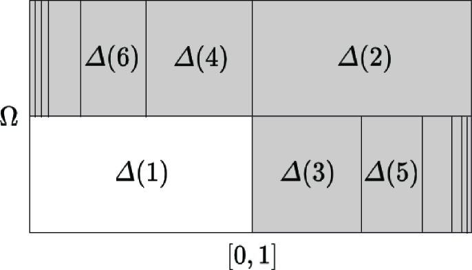
\inf_{\omega\in\Omega_{0}}\inf_{\Lambda_{\omega}}\liminf_{n\to\infty}\frac{1}{n}\log|(T_{\omega}^{n})^{\prime}|=0.

To control the effect of the neutral fixed point, we consider the inducing scheme $(\Lambda\setminus\varDelta(1),t_{\Lambda\setminus\varDelta(1)})$ of $R\colon\Lambda\to\Lambda$ and the associated induced system $\widehat{R}\colon\widehat{\Lambda}\to\widehat{\Lambda}$ , see Figure 2. Let us abbreviate $t_{\Lambda\setminus\varDelta(1)}$ as $t$ . Note that $t(\omega,x)$ is finite if and only if $T_{\omega}x\neq 0$ . The next lemma implies that the induced map $\widehat{R}$ is still not uniformly expanding. However, the lemma after the next one implies that $\widehat{R}^{2}$ is uniformly expanding.

Lemma 3.1.

Let $\omega\in\Omega$ satisfy $\omega_{1}=0$ , $\omega_{2}=1$ , $\omega_{3}=0$ . Then we have

\inf_{x\in\varDelta(2)}|(T_{\omega}^{t(\omega,x)})^{\prime}x|=1.

Proof.

Since $\inf_{(0,1]}|T_{0}^{\prime}|\geq 1$ and $\inf_{[0,1)}|T_{1}^{\prime}|\geq 1$ , we have $\inf_{x\in\varDelta(2)}|(T_{\omega}^{t(\omega,x)})^{\prime}x|\geq 1$ . By the hypothesis on $\omega$ and $T_{0}1=0$ , we have $\lim_{x\to 1-0}t(\omega,x)=2$ . Using this and the monotonicity of $|T_{0}^{\prime}|$ on $\varDelta(2)$ and that of $|T_{1}^{\prime}|$ on $\varDelta(1)$ , we obtain $\inf_{x\in\varDelta(2)}|(T_{\omega}^{t(\omega,x)})^{\prime}x|\leq\lim_{x\to 1-0}|(T_{1}\circ T_{0})^{\prime}x|=1$ . ∎

Lemma 3.2.

If $(\omega,x)\in\Lambda\setminus\varDelta(1)$ , $t(\omega,x)$ and $t(\widehat{R}(\omega,x))$ are finite and $a_{i}(\omega,x)=a_{i}(\varrho,y)$ for $i=1,\ldots,t(\omega,x)+t(\widehat{R}(\omega,x))$ , then

|(T_{\omega}^{t(\omega,x)+t(\widehat{R}(\omega,x))})^{\prime}y|\geq|(T_{\omega}^{t(\omega,x)+t(\widehat{R}(\omega,x))-1})^{\prime}(T_{\omega}y)|\geq\frac{9}{4}.

Proof.

From the definitions of $T_{0}$ and $T_{1}$ , $\inf_{(0,1]}|T^{\prime}_{0}|\geq 1$ , $\inf_{[0,1)}|T^{\prime}_{1}|\geq 1$ , the monotonicity of $|T_{0}|$ on $(0,1]$ and that of $|T_{1}^{\prime}|$ on $[0,1)$ , if $(\omega,x)\notin\varDelta(2)$ then

(T_{\omega}^{t(\omega,x)+t(\widehat{R}(\omega,x))})^{\prime}y|\geq|T_{\omega_{1}}^{\prime}y|\geq\left|T_{0}^{\prime}\left(\frac{1}{2}\right)\right|>\frac{9}{4}.

If $(\omega,x)\in\varDelta(2)$ and $T_{\omega}^{t(\omega,x)}x\in[1/2,1)$ then

(T_{\omega}^{t(\omega,x)+t(\widehat{R}(\omega,x))})^{\prime}y|\geq|T_{t(\omega,x)}^{\prime}y|\geq\left|T_{1}^{\prime}\left(\frac{1}{3}\right)\right|=\frac{9}{4}.

If $(\omega,x)\in\varDelta(2)$ and $T_{\omega}^{t(\omega,x)}x\in(0,1/2)$ then

(T_{\omega}^{t(\omega,x)+t(\widehat{R}(\omega,x))})^{\prime}y|\geq|T^{\prime}(T_{\omega}^{t(\omega,x)}y)|\geq\left|T_{0}^{\prime}\left(\frac{1}{2}\right)\right|>\frac{9}{4}.

Hence the desired inequality holds. ∎

Lemma 3.3 (Uniform decay of cylinders).

There exists $K\geq 1$ such that for every $n\in\mathbb{N}$ and every $a_{1}\cdots a_{n}\in\mathbb{N}^{n}$ ,

|J(a_{1}\cdots a_{n})|\leq\frac{K}{\sqrt{n}}.

Proof.

Take an integer $M\geq 4$ such that for every $n\geq M$ ,

(3.4)

\left(\frac{9}{4}\right)^{-\sqrt{n}/2+1}\leq\frac{1}{\sqrt{n}}.

Set $K=\sqrt{M}/2$ . Clearly we have $|J(k)|\leq 1/2$ for every $k\in\mathbb{N}$ . Hence, for every $1\leq n\leq M$ and every $a_{1}\cdots a_{n}\in\mathbb{N}^{n}$ we have $|J(a_{1}\cdots a_{n})|\leq 1/2=K/\sqrt{M}\leq K/\sqrt{n}$ as required.

Let $n\geq M+1$ and $a_{1}\cdots a_{n}\in\mathbb{N}^{n}$ . We may assume $a_{1}\cdots a_{n}$ contains $1$ , for otherwise a direct calculation shows $|J(a_{1}\cdots a_{n})|\leq 1/(n+1)$ . Let $N\geq 1$ denote the total number of blocks of consecutive $1$ s in $a_{1}\cdots a_{n}$ . A block of length not exceeding $\sqrt{n}$ is called a short block. A block which is not short is called a long block. If $N\geq\sqrt{n}/2$ , then Lemma 3.2 implies $|J(a_{1}\cdots a_{n})|\leq(9/4)^{-\sqrt{n}/2+1}$ . This and (3.4) together yield the desired inequality.

Suppose $N<\sqrt{n}/2$ . If there is no long block, then $\#\{1\leq i\leq n\colon a_{i}\neq 1\}\geq n-\sqrt{n}N>n/2$ . Let $j=\min\{i\geq 1\colon a_{i}\neq 1\}$ and $k=\max\{i\geq 1\colon a_{i}\neq 1\}$ . Define $(\omega_{i})_{i\in\mathbb{N}}\in\Omega$ by $\omega_{i}\equiv a_{i}\mod 2$ . By the mean value theorem and Lemma 3.2, for some $\ell\geq 1$ and all $x\in T_{\omega}^{j-1}(J(a_{1}\cdots a_{n}))$ we have

\begin{split}1\geq&|T_{\theta^{j}\omega}^{k-j+1}\circ T_{\omega}^{j-1}(J(a_{1}\cdots a_{n}))|\\ =&|T_{\theta^{j}\omega}^{t(\theta^{j}\omega,x)+t(\widehat{R}(\theta^{j}\omega,x))+\cdots+t(\widehat{R}^{\ell-1}(\theta^{j}\omega,x))}\circ T_{\omega}^{j-1}(J(a_{1}\cdots a_{n}))|\\ \geq&\left(\frac{9}{4}\right)^{\lfloor\ell/2\rfloor}|T_{\omega}^{j-1}(J(a_{1}\cdots a_{n}))|\geq\left(\frac{9}{4}\right)^{\lfloor\ell/2\rfloor}|J(a_{1}\cdots a_{n})|.\end{split}

Since $\ell\geq\lfloor n/2\rfloor-1\geq n/2-2$ we have $\ell/2\geq n/4-1$ , and so $\lfloor\ell/2\rfloor\geq\lfloor n/4-1\rfloor=\lfloor n/4\rfloor-1$ . Combining this inequality with the above yields $|J(a_{1}\cdots a_{n})|\leq(9/4)^{-\lfloor n/4\rfloor+1}$ . By $n\geq M+1\geq 5$ and (3.4), we obtain $(9/4)^{-\lfloor n/4\rfloor+1}\leq(9/4)^{-\sqrt{n}/2+1}\leq 1/\sqrt{n}$ . If there is a long block, then there exists $1\leq j\leq n-1$ such that $a_{i}=1$ for $i=j,\ldots,j+\lfloor\sqrt{n}\rfloor-1$ , and thus $T_{\omega}^{j-1}(J(a_{1}\cdots a_{n}))\subset J(1^{\lfloor\sqrt{n}\rfloor})\subset[0,1/(\lfloor\sqrt{n}\rfloor+1)$ . By the mean value theorem we obtain $|J(a_{1}\cdots a_{n})|\leq 1/\sqrt{n}$ . ∎

3.3. Annealed geometric potential

We introduce a function $\varphi\colon(\Omega\times[0,1])\setminus E\to\mathbb{R}$ by

\varphi(\omega,x)=\log p(\omega_{1})-\log|T_{\omega_{1}}^{\prime}x|,

where

p(\omega_{1})=\begin{cases}1-p\ &\text{ if }\omega_{1}=0,\\ p\ &\text{ if }\omega_{1}=1.\end{cases}

Note that $\varphi$ is unbounded and $\sup\varphi<0.$ We call $\varphi$ an annealed geometric potential. For $n\in\mathbb{N}$ write $S_{n}\varphi$ for the Birkhoff sum $\sum_{i=0}^{n-1}\varphi\circ R^{i}$ , and put $S_{0}\varphi\equiv 0$ for convenience. The annealed geometric potential ties in with Theorem 1.2. For all $(\omega,x)\in\Lambda$ and all $n\in\mathbb{N}$ we have

\exp(S_{n}\varphi(\omega,x))=Q_{n}^{p}(\omega)|(T_{\omega}^{n})^{\prime}x|^{-1}.

Compare this formula with (1.5). The next distortion estimate is straight forward.

Lemma 3.4.

For all $n\in\mathbb{N}$ , $a_{1}\cdots a_{n}\in\mathbb{N}^{n}$ and any pair $(\omega,x),(\varrho,y)$ of points in $\varDelta(a_{1}\cdots a_{n})$ ,

S_{n}\varphi(\omega,x)-S_{n}\varphi(\varrho,y)\leq 2\sum_{i=1}^{n}|T^{i}_{\omega}x-T^{i}_{\varrho}y|.

Proof.

We have

S_{n}\varphi(\omega,x)-S_{n}\varphi(\varrho,y)=\log\frac{|(T_{\omega}^{n})^{\prime}y|}{|(T_{\omega}^{n})^{\prime}x|}=\log\frac{|(T_{\varrho}^{n})^{\prime}y|}{|(T_{\varrho}^{n})^{\prime}x|}.

Then the desired inequality follows from the chain rule and (3.1). ∎

For each $n\in\mathbb{N}$ define

D_{n}(\varphi)=\sup\{S_{n}\varphi(\omega,x)-S_{n}\varphi(\varrho,y)\colon a_{i}(\omega,x)=a_{i}(\varrho,y),\ i=1,\ldots,n\}.

Note that $D_{1}(\varphi)<\infty$ , and $D_{n}(\varphi)$ is decreasing in $n$ .

Lemma 3.5.

We have $D_{n}(\varphi)=O(\sqrt{n})$ $(n\to\infty).$

Proof.

Let $n\in\mathbb{N}$ , $a_{1}\cdots a_{n}\in\mathbb{N}^{n}$ and let $(\omega,x),(\varrho,y)\in\varDelta(a_{1}\cdots a_{n})$ . Using Lemma 3.4 and then Lemma 3.3, we have

\begin{split}S_{n}\varphi(\omega,x)-S_{n}\varphi(\varphi,y)&\leq 2\sum_{i=1}^{n}|T_{\omega}^{i}x-T_{\varrho}^{i}y|\\ &\leq 2+2\sum_{i=1}^{n-1}|J(a_{i+1}\cdots a_{n})|\leq K\sum_{i=1}^{n}\frac{1}{\sqrt{n-i+1}}=O(\sqrt{n}),\end{split}

which implies the assertion of the lemma. ∎

3.4. Preliminary lemmas for the proof of Theorem 1.5

One key point in the proof of Theorem 1.5 is that the measure $\int_{\Omega}\tilde{\mu}^{\omega}_{n}(\cdot)dm_{p}(\omega)$ equals $\tilde{\mu}_{n}(\cdot)$ up to subexponential factors. To show this, we first provide subexponential bounds on the normalizing constants $Z_{\omega,n}$ in (1.2).

Lemma 3.6.

For all $\omega\in\Omega$ and $n\in\mathbb{N}$ we have

\exp(-D_{n}(\varphi))\leq Z_{\omega,n}\leq\exp(D_{n}(\varphi)).

In particular, $Z_{p,n}$ is finite for all $p\in(0,1)$ and all $n\in\mathbb{N}$ .

Proof.

Let $\omega\in\Omega$ , $n\in\mathbb{N}$ and let $a_{1}\cdots a_{n}\in\mathbb{N}^{\mathbb{N}}$ satisfy $\omega_{i}\equiv a_{i}$ mod $2$ for $i=1,\ldots,n$ . Clearly, $J(a_{1}\cdots a_{n})\cap{\rm Fix}(T_{\omega}^{n})$ is a singleton. Let $x(a_{1}\cdots a_{n})$ denote the element of this singleton. By the mean value theorem, for each $a_{1}\cdots a_{n}\in\mathbb{N}^{n}$ there exists $y(a_{1}\cdots a_{n})\in J(a_{1}\cdots a_{n})$ such that $|(T_{\omega}^{n})^{\prime}y(a_{1}\cdots a_{n})|^{-1}=|J(a_{1}\cdots a_{n})|.$ We have

\exp(-D_{n}(\varphi))|J(a_{1}\cdots a_{n})|\leq|(T_{\omega}^{n})^{\prime}x(a_{1}\cdots a_{n})|^{-1}\leq\exp(D_{n}(\varphi))|J(a_{1}\cdots a_{n})|.

Summing the first inequality over all relevant $a_{1}\cdots a_{n}$ gives

Z_{\omega,n}\geq\exp(-D_{n}(\varphi))\sum_{\begin{subarray}{c}a_{1}\cdots a_{n}\in\mathbb{N}^{n}\\ a_{i}\equiv\omega_{i}\mod 2\\ \ i=1,\ldots,n\end{subarray}}|J(a_{1}\cdots a_{n})|=\exp(-D_{n}(\varphi)),

as required. Summing the second inequality in the double inequalities over all relevant $a_{1}\cdots a_{n}$ yields the required upper bound. ∎

Lemma 3.7.

For any Borel subset $\mathcal{C}$ of $\mathcal{M}(\Lambda)$ and every $n\in\mathbb{N}$ ,

\exp(-2D_{n}(\varphi))\tilde{\mu}_{n}(\mathcal{C})\leq\int_{\Omega}\tilde{\mu}_{n}^{\omega}(\mathcal{C})dm_{p}(\omega)\leq\exp(2D_{n}(\varphi))\tilde{\mu}_{n}(\mathcal{C}).

Proof.

By Lemma 3.6, for all $\omega\in\Omega$ and all $n\in\mathbb{N}$ we have

(3.5)

\exp(-2D_{n}(\varphi))\leq{Z_{\omega,n}\Big{/}\int_{\Omega}Z_{\omega^{\prime},n}dm_{p}(\omega^{\prime})}\leq\exp(2D_{n}(\varphi)).

By the definitions of $\tilde{\mu}_{n}$ and $\tilde{\mu}_{n}^{\omega}$ , for any Borel subset $\mathcal{C}$ of $\mathcal{M}(\Lambda)$ and all $n\in\mathbb{N}$ ,

(3.6)

\begin{split}\tilde{\mu}_{n}(\mathcal{C})&=\frac{1}{Z_{p,n}}\sum_{\begin{subarray}{c}(\omega,x)\in{\rm Fix}(R^{n})\\ V_{n}^{R}(\omega,x)\in\mathcal{C}\end{subarray}}Q_{p}^{n}(\omega)|(T_{\omega}^{n})^{\prime}x|^{-1}\\ &=\int_{\Omega}\sum_{\begin{subarray}{c}x\in{\rm Fix}(T^{n}_{\omega})\\ V_{n}^{R}(\omega,x)\in\mathcal{C}\end{subarray}}|(T_{\omega}^{n})^{\prime}x|^{-1}dm_{p}(\omega)\Big{/}\int_{\Omega}Z_{\omega^{\prime},n}dm_{p}(\omega^{\prime})\\ &=\int_{\Omega}\tilde{\mu}_{n}^{\omega}(\mathcal{C})\left({Z_{\omega,n}\Big{/}\int_{\Omega}Z_{\omega^{\prime},n}dm_{p}(\omega^{\prime})}\right)dm_{p}(\omega).\end{split}

Combining (3.5) and (3.6) yields the desired inequality. ∎

The next lemma gives an upper bound for each closed subset of $\mathcal{M}(\Lambda)$ by the rate function $I_{p}$ , but is not sufficient for Theorem 1.5(a) since the set of permissible samples depends on the closed set in consideration.

Lemma 3.8.

For any closed subset $\mathcal{C}$ of $\mathcal{M}(\Lambda)$ , there exists a Borel subset $\Gamma(\mathcal{C})$ of $\Omega$ such that $m_{p}(\Gamma(\mathcal{C}))=1$ and for every $\omega\in\Gamma(\mathcal{C})$ ,

\limsup_{n\to\infty}\frac{1}{n}\log\tilde{\mu}_{n}^{\omega}(\mathcal{C})\leq-\inf_{\mathcal{C}}I_{p}.

Proof.

Let $\mathcal{C}$ be a closed subset of $\mathcal{M}(\Lambda)$ . We may assume $\inf_{\mathcal{C}}I_{p}>0$ , for otherwise the inequality is obvious. We first consider the case $\inf_{\mathcal{C}}I_{p}<\infty$ . For $\varepsilon\in(0,1)$ and $n\geq 1$ , set

\Omega_{\varepsilon,n}=\left\{\omega\in\Omega\colon\tilde{\mu}_{n}^{\omega}(\mathcal{C})\geq\exp\left(-n(1-\varepsilon)\inf_{\mathcal{C}}I_{p}\right)\right\}.

By Markov’s inequality and the second inequality in Lemma 3.7,

\begin{split}m_{p}(\Omega_{\varepsilon,n})&\leq\exp\left(n(1-\varepsilon)\inf_{\mathcal{C}}I_{p}\right)\int_{\Omega}\tilde{\mu}_{n}^{\omega}(\mathcal{C})dm_{p}(\omega)\\ &\leq\exp(2D_{n}(\varphi))\exp\left(n(1-\varepsilon)\inf_{\mathcal{C}}I_{p}\right)\tilde{\mu}_{n}(\mathcal{C}).\end{split}

By the LDP in Theorem 1.4(a), $m_{p}(\Omega_{\varepsilon,n})$ decays exponentially as $n$ increases. By Borel-Cantelli’s lemma, the inequality $\tilde{\mu}_{n}^{\omega}(\mathcal{C})\geq\exp(-n(1-\varepsilon)\inf_{\mathcal{C}}I_{p})$ holds only for finitely many $n$ for $m_{p}$ -almost every $\omega\in\Omega.$ Since $\varepsilon\in(0,1)$ is arbitrary, we obtain the desired inequality for $m_{p}$ -almost every $\omega\in\Omega$ .

To treat the remaining case $\inf_{\mathcal{C}}I_{p}=\infty$ , for $k,n\in\mathbb{N}$ we set

\Omega_{k,n}=\left\{\omega\in\Omega\colon\tilde{\mu}_{n}^{\omega}(\mathcal{C})\geq e^{-kn}\right\}.

By Markov’s inequality and Lemma 3.7,

m_{p}(\Omega_{k,n})\leq e^{kn}\int_{\Omega}\tilde{\mu}_{n}^{\omega}(\mathcal{C})dm_{p}(\omega)\leq\exp(2D_{n}(\varphi))e^{kn}\tilde{\mu}_{n}(\mathcal{C}).

Since $\mathcal{C}$ is closed, the LDP in Theorem 1.4(a) gives $\limsup_{n}(1/n)\log\tilde{\mu}_{n}(\mathcal{C})\leq-\inf_{\mathcal{C}}I_{p}=-\infty$ . Hence $m_{p}(\Omega_{k,n})$ decays exponentially as $n$ increases. By Borel-Cantelli’s lemma, there exists a Borel subset $\Gamma_{k}(\mathcal{C})$ of $\Omega$ such that $m_{p}(\Gamma_{k}(\mathcal{C}))=1$ , and for any $\omega\in\Gamma_{k}(\mathcal{C})$ the inequality $\tilde{\mu}_{n}^{\omega}(\mathcal{C})\geq e^{-kn}$ holds only for finitely many $n$ . Put $\Gamma(\mathcal{C})=\bigcap_{k=1}^{\infty}\Gamma_{k}(\mathcal{C})$ . We have $m_{p}(\Gamma(\mathcal{C}))=1$ , and $\limsup_{n}(1/n)\log\tilde{\mu}_{n}^{\omega}(\mathcal{C})=-\infty=-\inf_{\mathcal{C}}I_{p}$ for all $\omega\in\Gamma(\mathcal{C})$ as required. ∎

Since $\mathcal{M}(\Lambda)$ is non-compact, we need the following auxiliary lemma that leads to the exponential tightness of $(\tilde{\mu}^{\omega}_{n})_{n=1}^{\infty}$ as in Proposition 1.5(a).

Lemma 3.9.

For any $L>0$ there exists a compact subset $\mathcal{K}_{L}$ of $\mathcal{M}(\Lambda)$ and a Borel subset $\Gamma_{L}$ of $\Omega$ such that $m_{p}(\Gamma_{L})=1$ and for every $\omega\in\Gamma_{L}$ ,

\limsup_{n\to\infty}\frac{1}{n}\log\tilde{\mu}^{\omega}_{n}(\mathcal{M}(\Lambda)\setminus\mathcal{K}_{L})\leq-L.

Proof.

By the exponential tightness of $(\tilde{\mu}_{n})_{n=1}^{\infty}$ in Theorem 1.4(a), for any $L>0$ there is a compact subset $\mathcal{K}_{L}$ of $\mathcal{M}(\Lambda)$ such that

(3.7)

\limsup_{n\to\infty}\frac{1}{n}\log\tilde{\mu}_{n}(\mathcal{M}(\Lambda)\setminus\mathcal{K}_{L})\leq-2L.

For $n\in\mathbb{N}$ , set

\Omega_{L,n}=\left\{\omega\in\Omega\colon\tilde{\mu}_{n}^{\omega}(\mathcal{M}(\Lambda)\setminus\mathcal{K}_{L})\geq e^{-Ln}\right\}.

By Markov’s inequality and Lemma 3.7,

m_{p}(\Omega_{L,n})\leq e^{Ln}\int_{\Omega}\tilde{\mu}_{n}^{\omega}(\mathcal{M}(\Lambda)\setminus\mathcal{K}_{L})dm_{p}(\omega)\\ \leq\exp(2D_{n}(\varphi))e^{Ln}\tilde{\mu}_{n}(\mathcal{M}(\Lambda)\setminus\mathcal{K}_{L}).

By Lemma 3.5 and (3.7), $m_{p}(\Omega_{L,n})$ decays exponentially as $n$ increases. By Borel-Cantelli’s lemma, the number of those $n\in\mathbb{N}$ with $\tilde{\mu}_{n}^{\omega}(\mathcal{M}(\Lambda)\setminus\mathcal{K}_{L})\geq e^{-Ln}$ is finite for $m_{p}$ -almost every $\omega\in\Omega.$ ∎

3.5. Proof of Theorem 1.5

We fix a metric on $\mathcal{M}(\Lambda)$ that generates the weak* topology, and a countable dense subset $\mathcal{D}$ of on $\mathcal{M}(\Lambda)$ . For $\mu\in\mathcal{D}$ , $L\in\mathbb{N}$ let $B(\mu,1/L)$ denote the closed ball of radius $1/L$ about $\mu$ . By Lemma 3.8, there exists a Borel subset $\Gamma(B(\mu,1/L))$ of $\Omega$ with full $m_{p}$ -measure such that if $\omega\in\Gamma(B(\mu,1/L))$ then

(3.8)

\limsup_{n\to\infty}\frac{1}{n}\log\tilde{\mu}_{n}^{\omega}(B(\mu,1/L))\leq-\inf_{B(\mu,1/L)}I_{p}.

In view of Lemma 3.9, we fix an increasing sequence $(\mathcal{K}_{L})_{L=1}^{\infty}$ of compact subsets of $\mathcal{M}(\Lambda)$ and a sequence $(\Gamma_{L})_{L=1}^{\infty}$ of Borel subsets of $\Omega$ with full $m_{p}$ -measure such that $\bigcup_{L=1}^{\infty}\mathcal{K}_{L}=\mathcal{M}(\Lambda)$ , and for all $L\in\mathbb{N}$ and all $\omega\in\Gamma_{L}$ ,

(3.9)

\limsup_{n\to\infty}\frac{1}{n}\log\tilde{\mu}^{\omega}_{n}(\mathcal{M}(\Lambda)\setminus\mathcal{K}_{L})\leq-L.

We set

\Gamma=\left(\bigcap_{\mu\in\mathcal{D}}\bigcap_{L=1}^{\infty}\Gamma(B(\mu,1/L))\right)\cap\left(\bigcap_{L=1}^{\infty}\Gamma_{L}\right).

Clearly we have $m_{p}(\Gamma)=1$ . If $\omega\in\Gamma$ , then $(\tilde{\mu}_{n}^{\omega})_{n=1}^{\infty}$ is exponentially tight by (3.9).

Let $\mathcal{C}$ be a non-empty closed subset of $\mathcal{M}(\Lambda)$ and let $L\in\mathbb{N}$ . Let $\mathcal{G}$ be an open subset of $\mathcal{M}(\Lambda)$ that contains $\mathcal{C}\cap\mathcal{K}_{L}$ . Since $\mathcal{C}\cap\mathcal{K}_{L}$ is compact, there exists a finite subset $\{\mu_{1},\ldots,\mu_{s}\}$ of $\mathcal{D}$ and $L_{1},\ldots,L_{s}\in\mathbb{N}$ such that $\mathcal{C}\cap\mathcal{K}_{L}\subset\bigcup_{i=1}^{s}B(\mu_{i},1/L_{i})\subset\mathcal{G}$ . By (3.8) applied to each of these closed balls, we have

\begin{split}\limsup_{n\to\infty}\frac{1}{n}\log\tilde{\mu}_{n}^{\omega}(\mathcal{C}\cap\mathcal{K}_{L})&\leq\max_{1\leq i\leq s}\limsup_{n\to\infty}\frac{1}{n}\log\tilde{\mu}_{n}^{\omega}(B(\mu_{i},1/L_{i}))\\ &\leq\max_{1\leq i\leq s}\left(-\inf_{B(\mu_{i},1/L_{i})}I_{p}\right)\leq-\inf_{\mathcal{G}}I_{p}.\end{split}

Since $\mathcal{G}$ is an arbitrary open set containing $\mathcal{C}\cap\mathcal{K}_{L}$ and $I_{p}$ is lower semicontinuous,

(3.10)

\limsup_{n\to\infty}\frac{1}{n}\log\tilde{\mu}_{n}^{\omega}(\mathcal{C}\cap\mathcal{K}_{L})\leq-\inf_{\mathcal{C}\cap\mathcal{K}_{L}}I_{p}.

From (3.9) and (3.10), for every $\omega\in\Gamma$ we obtain

(3.11)

\limsup_{n\to\infty}\frac{1}{n}\log\tilde{\mu}^{\omega}_{n}(\mathcal{C})\leq\max\left\{-\inf_{\mathcal{C}\cap\mathcal{K}_{L}}I_{p},-L\right\}.

If $L\geq\inf_{\mathcal{C}\cap\mathcal{K}_{L}}I_{p}$ , then (3.11) yields

\limsup_{n\to\infty}\frac{1}{n}\log\tilde{\mu}^{\omega}_{n}(\mathcal{C})\leq-\inf_{\mathcal{C}\cap\mathcal{K}_{L}}I_{p}\leq-\inf_{\mathcal{C}}I_{p}.

Combining this with (3.9) we obtain the desired inequality. If $L<\inf_{\mathcal{C}\cap\mathcal{K}_{L}}I_{p}$ for all $L\in\mathbb{N}$ , then we obtain $\inf_{\mathcal{C}}I_{p}=\infty$ since $(\mathcal{K}_{L})_{L=1}^{\infty}$ is increasing and $\bigcup_{L=1}^{\infty}\mathcal{K}_{L}=\mathcal{M}(\Lambda)$ . Moreover, (3.11) yields $\limsup_{n}(1/n)\log\tilde{\mu}^{\omega}_{n}(\mathcal{C})=-\infty.$ The proof of Theorem 1.5(a) is complete.

By Theorem 1.5(a), $(\tilde{\mu}_{n}^{\omega})_{n=1}^{\infty}$ is tight for $m_{p}$ -almost every $\omega\in\Omega$ . By Prohorov’s theorem, it has a limit point. Let $(\tilde{\mu}_{n_{j}}^{\omega})_{j=1}^{\infty}$ be an arbitrary convergent subsequence of $(\tilde{\mu}_{n}^{\omega})_{n=1}^{\infty}$ with the limit measure $\tilde{\mu}^{\omega}$ . For a proof of Theorem 1.5(b) it suffices to show $\tilde{\mu}^{\omega}=\delta_{m_{p}\otimes\lambda_{p}}$ .

We fix a metric that generates the weak* topology on $\mathcal{M}(\Lambda)$ . Since $I_{p}$ is a good rate function by Theorem 1.4(a), for any $c>0$ the level set $I_{p}^{c}=\{\mu\in\mathcal{M}(\Lambda)\colon I_{p}(\mu)\leq c\}$ is compact. Let $\nu\in\mathcal{M}(\Lambda)\setminus\{m_{p}\otimes\lambda_{p}\}$ . By the last assertion of Proposition 2.3 we have $I_{p}(\nu)>0$ , and so $\nu\notin I_{p}^{I(\nu)/2}$ . Take $r>0$ such that the closed ball $B(\nu,r)$ of radius $r$ about $\nu$ in $\mathcal{M}(\Lambda)$ does not intersect $I_{p}^{I(\nu)/2}$ . By the weak* convergence of $(\tilde{\mu}_{n_{j}}^{\omega})_{j=1}^{\infty}$ to $\tilde{\mu}^{\omega}$ and the large deviations upper bound for closed sets in Theorem 1.5(a), we have

\begin{split}\tilde{\mu}^{\omega}({\rm int}(B(\nu,r)))&\leq\liminf_{j\to\infty}\tilde{\mu}_{n_{j}}^{\omega}({\rm int}(B(\nu,r)))\leq\limsup_{j\to\infty}\tilde{\mu}_{n_{j}}^{\omega}(B(\nu,r))\\ &\leq\limsup_{j\to\infty}\exp(-I_{p}(\nu)n_{j}/2)=0.\end{split}

Hence, the support of $\tilde{\mu}^{\omega}$ does not contain $\nu$ . Since $\nu$ is an arbitrary element of $\mathcal{M}(\Lambda)$ which is not $m_{p}\otimes\lambda_{p}$ , it follows that $\tilde{\mu}^{\omega}=\delta_{m_{p}\otimes\lambda_{p}}$ . The proof of Theorem 1.5(b) is complete. ∎

Remark 3.10.

Since $\mathcal{M}(\Lambda)$ is non-compact, the tightness in Theorem 1.5(a) was used in establishing the convergence in Theorem 1.5(b). Nevertheless, $\mathcal{M}(\Omega\times[0,1])$ is compact. By applying the Contraction Principle to the inclusion $\mathcal{M}(\Lambda)\hookrightarrow\mathcal{M}(\Omega\times[0,1])$ , one can transfer the LDP in Theorem 1.4(a) to the LDP for the sequence $(\tilde{\mu}_{n})_{n=1}^{\infty}$ viewed as a sequence in $\mathcal{M}^{2}(\Omega\times[0,1])$ . Using the latter LDP, one can establish a version of the upper bound in Theorem 1.5(a) for any closed subset of $\mathcal{M}(\Omega\times[0,1])$ , as well as the convergence of $(\tilde{\mu}_{n})_{n=1}^{\infty}$ to $\delta_{m_{p}\otimes\lambda_{p}}$ in $\mathcal{M}^{2}(\Omega\times[0,1])$ . These are actually sufficient for the proof of Theorem 1.1.

One merit of considering large deviations on the non-compact space $\mathcal{M}(\Lambda)$ rather than on $\mathcal{M}(\Omega\times[0,1])$ is that one can permit bounded continuous functions on $\Lambda$ that are naturally associated with the random continued fraction expansion (1.1), and do not have continuous extensions to $\Omega\times[0,1]$ . See Corollary 4.19 for details.

4. Establishing the LDP for the Gauss-Rényi map

This last section is mostly dedicated to the proof of Theorem 1.4. In §4.1 we summarize results on the thermodynamic formalism for the countable full shift. In §4.2 we consider an inducing scheme of the full shift and introduce a symbolic coding of the associated induced system. In §4.3 we recall the result of the second-named author [42] that give a sufficient condition for the level-2 LDP on periodic points in terms of induced potentials. We also recall the result in [40] on the uniqueness of minimizer of the rate function. In order to implement all these results, in $\S$ 4.4 we show that the Gauss-Rényi map is topologically conjugate to the shift map on the countable full shift. In §4.5 we perform distortion estimates for an induced version of the annealed geometric potential $\varphi$ . In §4.6 we establish the existence and uniqueness of the equilibrium state for the symbolic version of the potential $\varphi$ , and show that this equilibrium state is the symbolic version of the measure $m_{p}\otimes\lambda_{p}$ . In §4.7 we complete the proof of Theorem 1.4. In §4.8 we state two corollaries of independent interest on annealed and quenched level-1 large deviations, and apply them to the problem of frequency of digits in the random continued fraction expansion.

4.1. Thermodynamic formalism for the countable full shift

Consider the countable full shift

(4.1)

\mathbb{N}^{\mathbb{N}}=\{z=(z_{n})_{n=1}^{\infty}\colon z_{n}\in\mathbb{N}\text{ for }n\in\mathbb{N}\},

which is the cartesian product topological space of the discrete space $\mathbb{N}$ . We introduce main constituent components of the thermodynamic formalism for the countable full shift (4.1), and state a variational principle and a relationship between equilibrium states and Gibbs states. Our main reference is [27] that contains results on countable Markov shifts which are not necessarily the full shift.

The left shift $\sigma\colon\mathbb{N}^{\mathbb{N}}\to\mathbb{N}^{\mathbb{N}}$ given by $\sigma(z_{n})_{n=1}^{\infty}=(z_{n+1})_{n=1}^{\infty}$ is continuous. For $n\in\mathbb{N}$ and $a_{1}\cdots a_{n}\in\mathbb{N}^{n}$ , define an $n$ -cylinder

[a_{1}\cdots a_{n}]=\{z\in\mathbb{N}^{\mathbb{N}}\colon z_{i}=a_{i}\text{ for }i=1,\ldots,n\}.

Let $\mathcal{M}(\mathbb{N}^{\mathbb{N}},\sigma)$ denote the set of $\sigma$ -invariant Borel probability measures. For each $\mu\in\mathcal{M}(\mathbb{N}^{\mathbb{N}},\sigma)$ , let $h(\mu)\in[0,\infty]$ denote the measure-theoretic entropy of $\mu$ with respect to $\sigma$ . Let $\phi\colon\mathbb{N}^{\mathbb{N}}\to\mathbb{R}$ be a function, called a potential. For each $n\in\mathbb{N}$ we write $S_{n}\phi$ for the Birkhoff sum $\sum_{i=0}^{n-1}\phi\circ\sigma^{i}$ , and introduce a pressure

P(\phi)=\lim_{n\to\infty}\frac{1}{n}\log\sum_{a_{1}\cdots a_{n}\in\mathbb{N}^{n}}\sup_{[a_{1}\cdots a_{n}]}\exp S_{n}\phi.

This limit exists by the sub-additivity, which is never $-\infty$ . We say:

•

$\phi$ is acceptable if it is uniformly continuous and satisfies

$\sup_{a\in\mathbb{N}}\left(\sup_{[a]}\phi-\inf_{[a]}\phi\right)<\infty;$

•

$\phi$ is locally Hölder continuous if there exist constants $K>0$ and $\gamma\in(0,1)$ such that ${\rm var}_{n}(\phi)\leq K\gamma^{n}$ , where

{\rm var}_{n}(\phi)=\sup\{\phi(z)-\phi(w)\colon z,w\in\mathbb{N}^{\mathbb{N}},\ z_{i}=w_{i}\ \text{ for }i=1,\ldots,n\}.

Let $\phi\colon\mathbb{N}^{\mathbb{N}}\to\mathbb{R}$ be acceptable and satisfy $P(\phi)<\infty$ . Then $\sup\phi$ is finite (see [27, Proposition 2.1.9]). Let

\mathcal{M}_{\phi}(\mathbb{N}^{\mathbb{N}},\sigma)=\left\{\mu\in\mathcal{M}(\mathbb{N}^{\mathbb{N}},\sigma)\colon\int\phi d\mu>-\infty\right\}.

By [27, Theorem 2.1.7], for any $\mu\in\mathcal{M}_{\phi}(\mathbb{N}^{\mathbb{N}},\sigma)$ we have $h(\mu)+\int\phi d\mu\leq P(\phi)<\infty$ , and so $h(\mu)<\infty$ . The following equality is known as the variational principle.

Proposition 4.1 ([27, Theorem 2.1.7, Theorem 2.1.8]).

Let $\phi\colon\mathbb{N}^{\mathbb{N}}\to\mathbb{R}$ be acceptable and satisfy $P(\phi)<\infty$ . Then

P(\phi)=\sup\left\{h(\mu)+\int\phi d\mu\colon\mu\in\mathcal{M}_{\phi}(\mathbb{N}^{\mathbb{N}},\sigma)\right\}.

Let $\phi\colon\mathbb{N}^{\mathbb{N}}\to\mathbb{R}$ be acceptable and satisfy $P(\phi)<\infty$ . A measure $\mu\in\mathcal{M}_{\phi}(\mathbb{N}^{\mathbb{N}},\sigma)$ is called an equilibrium state for the potential $\phi$ if

P(\phi)=h(\mu)+\int\phi d\mu.

A measure $\mu\in\mathcal{M}(\mathbb{N}^{\mathbb{N}})$ is called a Gibbs state for the potential $\phi$ if there exists a constant $K\geq 1$ such that for all $n\in\mathbb{N}$ , all $a_{1}\cdots a_{n}\in\mathbb{N}^{n}$ and all $x\in[a_{1}\cdots a_{n}]$ ,

K^{-1}\leq\frac{\mu([a_{1}\cdots a_{n}])}{\exp(S_{n}\phi(x)-P(\phi)n)}\leq K.

Proposition 4.2 ([27, Theorem 2.2.9, Corollary 2.7.5]).

Let $\phi\colon\mathbb{N}^{\mathbb{N}}\to\mathbb{R}$ be locally Hölder continuous and satisfy $P(\phi)<\infty$ . Then there exists a unique shift-invariant Gibbs state $\mu_{\phi}$ for $\phi$ . If $\int\phi d\mu_{\phi}>-\infty$ , then $\mu_{\phi}$ is the unique equilibrium state for $\phi$ .

4.2. Coding of the induced system

Consider the inducing scheme $(\mathbb{N}^{\mathbb{N}}\setminus[1],t_{\mathbb{N}^{\mathbb{N}}\setminus[1]})$ of the left shift $\sigma\colon\mathbb{N}^{\mathbb{N}}\to\mathbb{N}^{\mathbb{N}}$ . We show that the associated induced system $\widehat{\sigma}\colon{\widehat{\mathbb{N}}}^{\mathbb{N}}\to{\widehat{\mathbb{N}}}^{\mathbb{N}}$ is in a natural way topologically conjugate to the full shift over an infinite alphabet.

We introduce the empty word $\emptyset$ by the rule $\omega\emptyset=\omega=\emptyset\omega$ for any word $\omega$ from $\mathbb{N}$ . For each $n\in\mathbb{N}$ , write $1^{n}$ for $11\cdots 1\in\mathbb{N}^{n}$ , the $n$ -string of $1$ . We set $1^{0}=\emptyset$ for convenience. We introduce an infinite alphabet

(4.2)

\mathbb{M}=\left\{\bigcup_{b\in\mathbb{N}\setminus\{1\}}[a1^{n}b]\colon a\in\mathbb{N}\setminus\{1\}\text{ and }n\in\mathbb{N}\cup\{0\}\right\},

which is a collection of pairwise disjoint subsets of $\mathbb{N}^{\mathbb{N}}\setminus[1]$ . We endow $\mathbb{M}$ with the discrete topology, and introduce the countable full shift

(4.3)

{\mathbb{M}}^{\mathbb{N}}=\{(x_{n})_{n=1}^{\infty}\colon x_{n}\in\mathbb{M}\text{ for }n\in\mathbb{N}\},

which is the cartesian product topological space of $\mathbb{M}$ . Clearly $\mathbb{M}^{\mathbb{N}}$ is topologically isomorphic to $\mathbb{N}^{\mathbb{N}}$ . With a slight abuse of notation let $\sigma\colon{\mathbb{M}}^{\mathbb{N}}\to{\mathbb{M}}^{\mathbb{N}}$ denote the left shift.

We define a map $\iota\colon\mathbb{M}^{\mathbb{N}}\to{\widehat{\mathbb{N}}}^{\mathbb{N}}$ as follows. Let $(x_{n})_{n=1}^{\infty}\in\mathbb{M}^{\mathbb{N}}$ . By the definition of $\mathbb{M}$ in (4.2), for every $n\in\mathbb{N}$ we have $x_{n}=\bigcup_{b\in\mathbb{N}\setminus\{1\}}[a_{n}1^{j_{n}}b]$ where $a_{n}\in\mathbb{N}\setminus\{1\}$ and $j_{n}\in\mathbb{N}\cup\{0\}$ . We set

\iota((x_{n})_{n=1}^{\infty})\in\bigcap_{n=1}^{\infty}[a_{1}1^{j_{1}}a_{2}1^{j_{2}}\cdots a_{n}1^{j_{n}}].

Lemma 4.3.

The map $\iota$ is a homeomorphism, and satisfies $\iota\circ\sigma=\widehat{\sigma}\circ\iota$ .

Proof.

Clearly $\iota$ is continuous and injective. For every $a\in\mathbb{N}\setminus\{1\}$ and every $n\in\mathbb{N}\cup\{0\}$ , the set $\bigcup_{b\in\mathbb{N}\setminus\{1\}}[a1^{n}b]$ is mapped by $\widehat{\sigma}$ bijectively onto $\mathbb{N}^{\mathbb{N}}\setminus[1]$ . Moreover, the collection of sets of this form defines a partition of the set $\bigcup_{k=1}^{\infty}\{t=k\}$ , namely

\bigcup_{k=1}^{\infty}\{t=k\}=\bigcup_{a\in\mathbb{N}\setminus\{1\}}\bigcup_{n\in\mathbb{N}\cup\{0\}}\bigcup_{b\in\mathbb{N}\setminus\{1\}}[a1^{n}b].

All the unions are disjoint unions. It follows that $\iota(\mathbb{M}^{\mathbb{N}})=\widehat{\mathbb{N}}^{\mathbb{N}}$ . The last assertion follows from the definition of $\iota.$ ∎

4.3. Level-2 LDP for the countable full shift

Let $\phi\colon\mathbb{N}^{\mathbb{N}}\to\mathbb{R}$ be acceptable and satisfy $P(\phi)<\infty$ . We are concerned with the LDP a sequence $(\tilde{\nu}_{n})_{n=1}^{\infty}$ of Borel probability measures on $\mathcal{M}(\mathbb{N}^{\mathbb{N}})$ given by

(4.4)

\tilde{\nu}_{n}=\frac{1}{Z_{n}(\phi)}\sum_{x\in{\rm Fix}(\sigma^{n})}\exp(S_{n}\phi(x))\delta_{V_{n}^{\sigma}(x)},

where $V_{n}^{\sigma}(x)\in\mathcal{M}(\mathbb{N}^{\mathbb{N}})$ denotes the uniform probability distribution on the orbit $(\sigma^{i}x)_{i=0}^{n-1}$ , and $\delta_{V_{n}^{\sigma}(x)}$ denotes the Borel probability measure on $\mathcal{M}(\mathbb{N}^{\mathbb{N}})$ that is the unit point mass at $V_{n}^{\sigma}(x)$ , and $Z_{n}(\phi)$ denotes the normalizing constant. We introduce a free energy $F_{\phi}\colon\mathcal{M}(\mathbb{N}^{\mathbb{N}})\to[-\infty,0]$ by

F_{\phi}(\mu)=\begin{cases}h(\mu)+\int\phi d\mu&\text{ if $\mu\in\mathcal{M}_{\phi}(\mathbb{N}^{\mathbb{N}},\sigma)$},\\ -\infty&\text{ otherwise.}\end{cases}

The function $-F_{\phi}+P(\phi)$ is a natural candidate for the rate function of this LDP. However, this function may not be lower semicontinuous since the entropy function is not upper semicontinuous. Hence, we take the lower semicontinuous regularization of $-F_{\phi}+P(\phi)$ . Define $I_{\phi}\colon\mathcal{M}(\mathbb{N}^{\mathbb{N}})\to[0,\infty]$ by

(4.5)

I_{\phi}(\mu)=-\inf_{\mathcal{G}\ni\mu}\sup_{\nu\in\mathcal{G}}F_{\phi}(\nu)+P(\phi),

where the supremum is taken over all measures in an open subset $\mathcal{G}$ of $\mathcal{M}(\mathbb{N}^{\mathbb{N}})$ that contains $\mu$ , and the infimum is taken over all such open subsets. Then $I_{\phi}$ is lower semicontinuous and satisfies $I_{\phi}\leq-F_{\phi}+P(\phi)$ .

If there is a Gibbs state for the potential $\phi$ , then the LDP holds for $(\tilde{\nu}_{n})_{n=1}^{\infty}$ from the result in [38]. Due to the existence of the neutral fixed point of the Rényi map $T_{1}$ , the annealed Gauss-Rényi measure $\eta_{p}$ is not a Gibbs state for the potential $\psi$ (see Lemma 4.12). Hence [38] cannot be applied to $(\mathbb{N}^{\mathbb{N}},\psi)$ . Instead we apply the result in [42] on the LDP for $(\tilde{\nu}_{n})_{n=1}^{\infty}$ when a Gibbs state for $\phi$ does not exist.

Using the conjugacy $\iota$ in §4.2, we introduce a parametrized family of twisted induced potentials $\Phi_{\gamma}\colon{\mathbb{M}}^{\mathbb{N}}\to\mathbb{R}$ ( $\gamma\in\mathbb{R}$ ) by

(4.6)

\Phi_{\gamma}(\iota(x))=S_{t_{\mathbb{N}^{\mathbb{N}}\setminus[1]}(\iota(x))}\phi(\iota(x))-\gamma t_{\mathbb{N}^{\mathbb{N}}\setminus[1]}(\iota(x)).

Theorem 4.4 ([42, Theorem A]).

Let $\phi\colon\mathbb{N}^{\mathbb{N}}\to\mathbb{R}$ be acceptable and satisfy $P(\phi)<\infty$ . Suppose the twisted induced potentials $\Phi_{\gamma}\colon\mathbb{M}^{\mathbb{N}}\to\mathbb{R}$ $(\gamma\in\mathbb{R})$ are locally Hölder continuous, and there exists $\gamma_{0}\in\mathbb{R}$ such that $P(\Phi_{\gamma_{0}})=0$ . Then $(\tilde{\nu}_{n})_{n=1}^{\infty}$ is exponentially tight and satisfies the LDP with the good rate function $I_{\phi}$ .

The uniqueness of minimizer of the rate function $I_{\phi}$ does not follow from Theorem 4.4 and should be examined on a case-by-case basis. An ideal situation is that the shift-invariant Gibbs state for $\phi$ is unique, the equilibrium state for $\phi$ is unique, the minimizer of $I_{\phi}$ is unique, and all these three coincide. However this is not always the case. Under the hypothesis of Theorem 4.4, by virtue of Proposition 4.2 there exists a unique Gibbs state for the potential $\phi$ . If moreover $\phi$ is integrable against the Gibbs state, then it is the unique equilibrium state for $\phi$ , and clearly is a minimizer of $I_{\phi}$ . Conversely, a minimizer of $I_{\phi}$ may not be an equilibrium state for $\phi$ in general: an example of a potential $\phi\colon\mathbb{N}^{\mathbb{N}}\to\mathbb{R}$ can be found in [35] for which there is a Gibbs state $\mu\in\mathcal{M}(\mathbb{N}^{\mathbb{N}},\sigma)$ such that $I_{\phi}(\mu)=0$ and $\mu$ is not an equilibrium state since $\int\phi d\mu=-\infty$ .

Under additional hypothesis on the potential, one can show that any minimizer is an equilibrium state. We say $\phi\colon\mathbb{N}^{\mathbb{N}}\to\mathbb{R}$ is summable if $\sum_{k\in\mathbb{N}}\sup_{[k]}e^{\phi}$ is finite. If $\phi$ is summable, then $P(\phi)<\infty$ . Set

\beta_{\infty}(\phi)=\inf\left\{\beta\in\mathbb{R}\colon\text{$\beta\phi$ is summable}\right\}.

Proposition 4.5.

Let $\phi\colon\mathbb{N}^{\mathbb{N}}\to\mathbb{R}$ be uniformly continuous and summable with $\beta_{\infty}(\phi)<1$ . Then, any minimizer of $I_{\phi}$ is an equilibrium state for the potential $\phi$ .

A proof of this proposition is briefly outline as follows. By the definition (4.5), if $\mu$ is a minimizer of $I_{\phi}$ then there is a sequence $(\mu_{k})_{k=1}^{\infty}$ in $\mathcal{M}_{\phi}(\mathbb{N}^{\mathbb{N}},\sigma)$ that converges to $\mu$ in the weak* topology with $\lim_{k}F_{\phi}(\mu_{k})=0$ . Based on this information we show that $\mu$ is an equilibrium state for $\phi$ . The case $\lim_{k}h(\mu_{k})=0$ is easy to handle, while the case $\lim_{k}h(\mu_{k})=\infty$ (and hence $\lim_{k}\int\phi d\mu_{k}\to-\infty$ ) requires attention. A key ingredient in the latter case is the upper semicontinuity of the map $\mu_{k}\mapsto h(\mu_{k})/(-\int\phi d\mu_{k})$ , as proved in [40, Theorem 2.4] inspired by [14, Lemma 6.5].

Proof of Proposition 4.5.

The following proof is almost a repetition of the proof of [40, Theorem 2.1] for the reader’s convenience. Considering $\phi-P(\phi)$ instead of $\phi$ , we may assume $P(\phi)=0$ . Let $\mu\in\mathcal{M}(\mathbb{N}^{\mathbb{N}},\sigma)$ be a minimizer of $I_{\phi}$ . Since $\mathcal{M}(\mathbb{N}^{\mathbb{N}},\sigma)$ is a closed subset of $\mathcal{M}(\mathbb{N}^{\mathbb{N}},\sigma)$ , $\mu$ is shift-invariant. By the definition (4.5), there is a sequence $(\mu_{k})_{k=1}^{\infty}$ in $\mathcal{M}_{\phi}(\mathbb{N}^{\mathbb{N}},\sigma)$ that converges to $\mu$ in the weak* topology with $\lim_{k}F_{\phi}(\mu_{k})=0$ . By [40, Lemma 2.3], we have $\inf_{k}\int\phi d\mu_{k}>-\infty$ . By this and $\sup\phi<\infty$ , a simple upper semicontinuity argument as in [40, Remark 2.5] shows $\int\phi d\mu>-\infty$ . If $\liminf_{k}h(\mu_{k})=0$ , then for any subsequence $(\mu_{k_{j}})_{j=1}^{\infty}$ with $\lim_{j}h(\mu_{k_{j}})=0$ we have

0=\lim_{j\to\infty}F_{\phi}(\mu_{k_{j}})\leq\int\phi d\mu\leq h(\mu)+\int\phi d\mu=F_{\phi}(\mu).

Since $F_{\phi}(\mu)\leq P(\phi)=0$ , $\mu$ is an equilibrium state for $\phi$ . If $\liminf_{k}h(\mu_{k})>0$ , then we have $\liminf_{k}(-\int\phi d\mu_{k})>0$ and

0=\lim_{k\to\infty}F_{\phi}(\mu_{k})=\lim_{k\to\infty}\left(-\int\phi d\mu_{k}\right)\left(\frac{h(\mu_{k})}{-\int\phi d\mu_{k}}-1\right).

It follows that

\lim_{k\to\infty}\left(\frac{h(\mu_{k})}{-\int\phi d\mu_{k}}-1\right)=0.

We have $-\int\phi d\mu\geq h(\mu)$ . If $-\int\phi d\mu=0$ , then clearly $\mu$ is an equilibrium state for $\phi$ . If $-\int\phi d\mu>0$ , then by [40, Theorem 2.4] we have

\frac{h(\mu)}{-\int\phi d\mu}-1\geq 0,

namely $F_{\phi}(\mu)\geq 0$ . Since $F_{\phi}(\mu)\leq 0$ , $\mu$ is an equilibrium state for $\phi$ . The proof of Proposition 4.5 is complete. ∎

4.4. Symbolic coding of the Gauss-Rényi map

The next proposition allows us to introduce a symbolic representation of the Gauss-Rényi map.

Proposition 4.6.

The following statements hold.

(a)

For every $(a_{n})_{n\in\mathbb{N}}\in\mathbb{N}^{\mathbb{N}}$ we have $\bigcap_{n=1}^{\infty}\varDelta(a_{1}\cdots a_{n})=\{(\omega,x)\}\subset\Lambda$ , where $\omega_{n}\equiv a_{n}\mod 2$ , $C_{n}=(a_{n}+\omega_{n})/2+\omega_{n+1}$ and

x=\omega_{1}+\frac{\displaystyle{\hfill{(-1)^{\omega_{1}}}\hfill\;\vrule}}{\displaystyle{\vrule\;\hfill{C_{1}}\hfill}}+\frac{\displaystyle{\hfill{(-1)^{\omega_{2}}}\hfill\;\vrule}}{\displaystyle{\vrule\;\hfill{C_{2}}\hfill}}+\frac{\displaystyle{\hfill{(-1)^{\omega_{3}}}\hfill\;\vrule}}{\displaystyle{\vrule\;\hfill{C_{3}}\hfill}}+\cdots.

(b)

For every $(\omega,x)\in\Lambda$ we have $\{(\omega,x)\}=\bigcap_{n=1}^{\infty}\varDelta(a_{1}\cdots a_{n})$ , where $a_{n}=2C_{n}(\omega,x)+\omega_{n}-2\omega_{n+1}$ .

Proof.

As for (a), let $(a_{n})_{n\in\mathbb{N}}\in\mathbb{N}^{\mathbb{N}}$ . Define $(\omega_{n})_{n\in\mathbb{N}}\in\{0,1\}^{\mathbb{N}}$ by $\omega_{n}\equiv a_{n}\mod 2$ , and $C_{n}=(a_{n}+\omega_{n})/2+\omega_{n+1}$ for $n\in\mathbb{N}$ . Note that $(-1)^{\omega_{n+1}}+C_{n}\geq 1$ for every $n\in\mathbb{N}$ . By Lemma 2.2, the displayed continued fraction converges to a number $x\in[0,1]$ , and thus $(\omega,x)\in\bigcap_{n=1}^{\infty}\varDelta(a_{1}\cdots a_{n})$ . The algorithm described in §2.1 shows $\{(\omega,x)\}=\bigcap_{n=1}^{\infty}\varDelta(a_{1}\cdots a_{n})$ . Since $R^{n}(\omega,x)=(\theta^{n}\omega,T_{\omega}^{n}x)$ we have

T_{\omega}^{n}x=\omega_{n+1}+\frac{\displaystyle{\hfill{(-1)^{\omega_{n+1}}}\hfill\;\vrule}}{\displaystyle{\vrule\;\hfill{C_{n+1}}\hfill}}+\frac{\displaystyle{\hfill{(-1)^{\omega_{n+2}}}\hfill\;\vrule}}{\displaystyle{\vrule\;\hfill{C_{n+2}}\hfill}}+\frac{\displaystyle{\hfill{(-1)^{\omega_{n+3}}}\hfill\;\vrule}}{\displaystyle{\vrule\;\hfill{C_{n+3}}\hfill}}+\cdots.

Hence $(\omega,x)\in\Lambda$ holds.

To prove (b), let $(\omega,x)\in\Lambda$ . Define $a_{n}=2C_{n}(\omega,x)-\omega_{n}-2\omega_{n+1}$ for $n\in\mathbb{N}$ . We have $(-1)^{\omega_{n+1}}+C_{n}(\omega,x)\geq 1$ for every $n\in\mathbb{N}$ . Proposition 2.1(a) gives

x=\omega_{1}+\frac{\displaystyle{\hfill{(-1)^{\omega_{1}}}\hfill\;\vrule}}{\displaystyle{\vrule\;\hfill{C_{1}(\omega,x)}\hfill}}+\frac{\displaystyle{\hfill{(-1)^{\omega_{2}}}\hfill\;\vrule}}{\displaystyle{\vrule\;\hfill{C_{2}(\omega,x)}\hfill}}+\frac{\displaystyle{\hfill{(-1)^{\omega_{3}}}\hfill\;\vrule}}{\displaystyle{\vrule\;\hfill{C_{3}(\omega,x)}\hfill}}+\cdots,

which implies $(\omega,x)\in\bigcap_{n=1}^{\infty}\varDelta(a_{1}\cdots a_{n})$ . Proposition 4.6(a) yields $\{(\omega,x)\}=\bigcap_{n=1}^{\infty}\varDelta(a_{1}\cdots a_{n})$ . ∎

Define a coding map $\pi\colon\mathbb{N}^{\mathbb{N}}\to\Lambda$ by

(4.7)

\pi((z_{n})_{n=1}^{\infty})\in\bigcap_{n=1}^{\infty}\varDelta(z_{1}\cdots z_{n}).

By Proposition 4.6, $\pi$ is well-defined and surjective. Obviously $\pi$ is continuous, injective and satisfies $R\circ\pi=\pi\circ\sigma$ . It is not hard to show that $\pi$ maps Borel sets to Borel sets. We set

(4.8)

\eta_{p}=(m_{p}\otimes\lambda_{p})\circ\pi,

and call $\eta_{p}$ the annealed Gauss-Rényi measure. From (b) and (c) in Proposition 2.1, we have $\Lambda_{\omega}=(0,1)\setminus\mathbb{Q}$ for every $\omega\in\Omega_{0}$ . This implies $\Omega_{0}\times((0,1)\setminus\mathbb{Q})\subset\Lambda$ , and so $(m_{p}\otimes\lambda_{p})(\Lambda)=1$ . Hence $\eta_{p}$ is a probability. The measure $m_{p}\otimes\lambda_{p}$ is $R$ -invariant [23, Theorem 3.2] and by [23, Theorem 3.3] it is mixing. Hence $\eta_{p}$ is $\sigma$ -invariant and mixing.

By Lemma 4.3, the induced system $\widehat{\sigma}\colon{\widehat{\mathbb{N}}}^{\mathbb{N}}\to{\widehat{\mathbb{N}}}^{\mathbb{N}}$ is topologically conjugate to $\sigma\colon\mathbb{M}^{\mathbb{N}}\to\mathbb{M}^{\mathbb{N}}$ via $\iota$ . Since $R\colon\Lambda\to\Lambda$ is topologically conjugate to $\sigma\colon\mathbb{N}^{\mathbb{N}}\to\mathbb{N}^{\mathbb{N}}$ via $\pi$ , the two induced systems $\widehat{R}\colon\widehat{\Lambda}\to\widehat{\Lambda}$ and $\widehat{\sigma}\colon{\widehat{\mathbb{N}}}^{\mathbb{N}}\to{\widehat{\mathbb{N}}}^{\mathbb{N}}$ are topologically conjugate via $\pi$ . The three dynamical systems are summarized in the following diagram.

(4.9)

\begin{CD}\mathbb{M}^{\mathbb{N}}@>{\sigma}>{}>\mathbb{M}^{\mathbb{N}}\\ @V{\iota}V{}V@V{}V{\iota}V\\ {\widehat{\mathbb{N}}}^{\mathbb{N}}@>{\widehat{\sigma}}>{}>{\widehat{\mathbb{N}}}^{\mathbb{N}}\\ @V{\pi}V{}V@V{}V{\pi}V\\ \widehat{\Lambda}@>{\widehat{R}}>{}>\widehat{\Lambda}\\ \end{CD}

4.5. Refined distortion estimates

The distortion estimate in Lemma 3.4 does not suffice when $a_{1}\cdots a_{n}$ contains a long block of $1$ that contains $a_{n}$ . The next lemma provides refined estimates in this case.

Lemma 4.7.

There exists a constant $K>0$ such that if $n\in\mathbb{N}$ , $a_{i}=1$ for $i=1,\ldots,n$ and $a_{n+1}\neq 1$ then for any pair $(\omega,x),(\varrho,y)$ of points in $\varDelta(a_{1}\cdots a_{n+1})$ ,

S_{n}\varphi(\omega,x)-S_{n}\varphi(\varrho,y)\leq\begin{cases}K|T_{\omega}^{n}x-T_{\varrho}^{n}y|&\text{ if }a_{n+1}\in\mathbb{N}_{1},\\ K|T_{\omega}^{n}x-T_{\varrho}^{n}y|^{\frac{1}{2}}&\text{ if }a_{n+1}\in\mathbb{N}_{0}.\end{cases}

Proof.

Let $n\in\mathbb{N}$ and suppose $a_{i}=1$ for $i=1,\ldots,n$ and $a_{n+1}\neq 1$ . For $i=0,\ldots,n$ put

q_{i}=\begin{cases}\vskip 3.69885pt\displaystyle{\frac{1}{i+2}}&\text{ if }a_{n+1}\in\mathbb{N}_{1},\\ \displaystyle{\frac{2}{2i+a_{n+1}}}&\text{ if }a_{n+1}\in\mathbb{N}_{0},\end{cases}

and $J_{i}=\left[q_{i+1},q_{i}\right)$ . Let $(\omega,x),(\varrho,y)\in\varDelta(a_{1}\cdots a_{n+1})$ . We have $T_{1}(q_{i+1})=q_{i}$ for $i=0,\ldots,n-1$ and $x,y\in J_{n-1}$ . If $a_{n+1}\in\mathbb{N}_{1}$ then by Lemma 4.8 below applied to $f=T_{1}|[0,1/2)$ , there exists a uniform constant $K_{1}>0$ such that

(4.10)

S_{n}\varphi(\omega,x)-S_{n}\varphi(\varrho,y)\leq K_{1}|T_{\omega}^{n}x-T_{\varrho}^{n}y|.

If $a_{n+1}\in\mathbb{N}_{0}$ then we have

(4.11)

|J_{0}|=\frac{4}{a_{n+1}^{2}+2a_{n+1}}\ \text{ and }\ \sum_{i=0}^{n-1}|J_{i}|\leq\frac{2}{a_{n+1}}.

By Lemma 4.8 below applied to the restriction $f=T_{1}|_{[0,2/a_{n+1})}$ , there exists a uniform constant $K_{2}>0$ such that

S_{n}\varphi(\omega,x)-S_{n}\varphi(\varrho,y)\leq K_{2}\frac{|T_{\omega}^{n}x-T_{\varrho}^{n}y|}{|J_{0}|}\sum_{i=0}^{n-1}|J_{i}|.

Since $R^{n}(\omega,x),R^{n}(\varrho,y)\in\varDelta(a_{n+1})$ , the points $T_{\omega}^{n}x$ , $T_{\varrho}^{n}y$ belong to the closure of $J_{0}$ , and thus $|T_{\omega}^{n}x-T_{\varrho}^{n}y|/|J_{0}|\leq 1$ . By this and (4.11),

(4.12)

\begin{split}S_{n}\varphi(\omega,x)-S_{n}\varphi(\varrho,y)&\leq K_{2}\frac{|T_{\omega}^{n}x-T_{\varrho}^{n}y|}{|J_{0}|}\sum_{i=0}^{n-1}|J_{i}|\\ &\leq K_{2}\frac{|T_{\omega}^{n}x-T_{\varrho}^{n}y|^{\frac{1}{2}}}{|J_{0}|^{\frac{1}{2}}}\sum_{i=0}^{n-1}|J_{i}|\\ &\leq K_{2}\frac{\sqrt{a_{n+1}^{2}+2a_{n+1}}}{a_{n+1}}|T_{\omega}^{n}x-T_{\varrho}^{n}y|^{\frac{1}{2}}\\ &\leq\sqrt{2}K_{2}|T_{\omega}^{n}x-T_{\varrho}^{n}y|^{\frac{1}{2}}.\end{split}

By (4.10) and (4.12), taking $K=\max\{K_{1},\sqrt{2}K_{2}\}$ yields the desired inequalities. ∎

The next general lemma on distortions for iterations of an interval map with a neutral fixed point was shown in the proof of [20, Lemma 5.3].

Lemma 4.8 (cf. [20, Lemma 5.3]).

Let $r>0$ and let $f\colon[0,r)\to\mathbb{R}$ be a $C^{2}$ map satisfying $f0=0$ , $f^{\prime}0=1$ and $f^{\prime}x>1$ for all $x\in(0,r)$ . There exists a constant $K>0$ such that for every $n\in\mathbb{N}$ and any pair $x,y$ of points in $J_{n-1}$ ,

\log\frac{|(f^{n})^{\prime}y|}{|(f^{n})^{\prime}x|}\leq K|f^{n}x-f^{n}y|\sum_{i=0}^{n-1}\frac{|J_{i}|}{|J_{0}|},

where $q_{0}=r$ , $fq_{i+1}=q_{i}$ and $J_{i}=[q_{i+1},q_{i})$ for $i=0,\ldots,n-1$ .

We now proceed to distortion estimates of an induced potential. Notice that

\widehat{\Lambda}=(\Lambda\setminus\varDelta(1))\setminus\bigcup_{n=1}^{\infty}R^{-n}((1^{\infty},0)).

Define an induced annealed geometric potential $\widehat{\varphi}\colon\widehat{\Lambda}\to\mathbb{R}$ by

\widehat{\varphi}(\omega,x)=S_{t(\omega,x)}\varphi(\omega,x).

For a pair $(\omega,x),(\varrho,y)$ of distinct points in $\widehat{\Lambda}$ contained in the same $1$ -cylinder, we introduce their separation time

s((\omega,x),(\varrho,y))=\min\{n\geq 1\colon a_{1}(\widehat{R}^{n}(\omega,x))\neq a_{1}(\widehat{R}^{n}(\varrho,y))\}.

Note that $s((\omega,x),(\varrho,y))\geq 2$ implies $t(\omega,x)=t(\varrho,y)$ . We evaluate the quantity

\widehat{\varphi}(\omega,x)-\widehat{\varphi}(\varrho,y)=\log\frac{|(T_{\omega}^{t(\omega,x)})^{\prime}y|}{|(T_{\omega}^{t(\omega,x)})^{\prime}x|}.

Lemma 4.9.

There exist constants $K>0$ and $\tau\in(0,1)$ such that for any pair $(\omega,x),(\varrho,y)$ of points in $\widehat{\Lambda}$ with $s((\omega,x),(\varrho,y))\geq 2$ ,

\widehat{\varphi}(\omega,x)-\widehat{\varphi}(\varrho,y)\leq K\tau^{s((x,\omega),(\varrho,y))}.

Proof.

For $(\omega,x),(\varrho,y)\in\widehat{\Lambda}$ as in the statement, put

k=\min\{i\geq 1\colon R^{i}(\omega,x)\in\varDelta(1)\}\text{ and }n=t(\omega,x),

and decompose $R^{n}=R^{n-k}\circ R^{k}$ . We estimate contributions from the first $k$ iteration and the remaining $n-k$ iteration separately. Lemma 3.4 gives

(4.13)

S_{k}\varphi(\omega,x)-S_{k}\varphi(\varrho,y)\leq 2|T^{k}_{\omega}x-T^{k}_{\varrho}y|\ \text{ if $k=1$}.

By Lemma 3.4 and Lemma 3.2,

(4.14)

\begin{split}S_{k}\varphi(\omega,x)-S_{k}\varphi(\varrho,y)&\leq 2\sum_{i=1}^{k}|T^{i}_{\omega}x-T^{i}_{\varrho}y|\\ &\leq 2\left(1+\sum_{i=1}^{k-1}\left(\frac{4}{9}\right)^{\lfloor(k-i)/2\rfloor}\right)|T^{k}_{\omega}x-T^{k}_{\varrho}y|\ \text{ if $k>1$}.\end{split}

Put $\tau=(4/9)^{\frac{1}{4}}\in(0,1)$ and $K_{0}=2\left(1+\sum_{i=0}^{\infty}(4/9)^{\lfloor i/2\rfloor}\right)$ . By the mean value theorem, there exists $(\theta^{n}\omega,z)\in\varDelta(a_{n+1}(\omega,x))$ such that

\begin{split}|T_{\omega}^{k}x-T_{\omega}^{k}y|&\leq|T_{\omega}^{n}x-T_{\omega}^{n}y|\\ &=\frac{|T_{\omega}^{\sum_{i=0}^{s((\omega,x),(\varrho,y))-1}t(\widehat{R}^{i}(\omega,x))}x-T_{\omega}^{\sum_{i=0}^{s((\omega,x),(\varrho,y))-1}t(\widehat{R}^{i}(\omega,x))}y|}{|(T_{\theta^{n}\omega}^{\sum_{i=0}^{s((\omega,x),(\varrho,y))-1}t(\widehat{R}^{i}(\omega,x))-n})^{\prime}z|}.\end{split}

By Lemma 3.2, there exists a uniform constant $K_{1}>0$ such that

(4.15)

|T_{\omega}^{n}x-T_{\omega}^{n}y|\leq\frac{1}{|(T_{\theta\omega}^{\sum_{i=0}^{s((\omega,x),(\varrho,y))-1}t(\widehat{R}^{i}(\omega,x))-n})^{\prime}z|}\leq K_{1}\tau^{2s((\omega,x),(\varrho,y))}.

By Lemma 4.7, there exists a uniform constant $K_{2}>0$ such that

(4.16)

|S_{n-k}\varphi(R^{k}(\omega,x))-S_{n-k}\varphi(R^{k}(\varrho,y))|\leq K_{2}|T_{\omega}^{n}x-T_{\varrho}^{n}y|^{\frac{1}{2}}.

Combining (4.13), (4.14), (4.15) and (4.16) we obtain

\begin{split}\widehat{\varphi}(\omega,x)-\widehat{\varphi}(\varrho,y)&=S_{n}\varphi(\omega,x)-S_{n}\varphi(\varrho,y)\\ &\leq|S_{k}\varphi(\omega,x)-S_{k}\varphi(\varrho,y)|+|S_{n-k}\varphi(R^{k}(\omega,x))-S_{n-k}\varphi(R^{k}(\varrho,y))|\\ &\leq K_{0}K_{1}\tau^{2s((\omega,x),(\varrho,y))}+K_{2}|T_{\omega}^{n}x-T_{\varrho}^{n}y|^{\frac{1}{2}}\\ &\leq(K_{0}K_{1}+K_{2}\sqrt{K_{1}})\tau^{s((\omega,x),(\varrho,y))}.\end{split}

Setting $K=K_{0}K_{1}+K_{2}\sqrt{K_{1}}$ yields the desired inequality. ∎

For each $n\in\mathbb{N}$ define

V_{n}(\widehat{\varphi})=\sup\{\widehat{\varphi}(\omega,x)-\widehat{\varphi}(\varrho,y)\colon(\omega,x),(\varrho,y)\in\widehat{\Lambda},\ s((\omega,x),(\varrho,y))\geq n\}.

Corollary 4.10.

There exist constants $K>0$ and $\gamma\in(0,1)$ such that for every $n\geq 1$ we have $V_{n}(\widehat{\varphi})\leq K\gamma^{n}$ .

Proof.

Follows from Lemma 4.7 and Lemma 4.9.∎

4.6. Variational characterization of the annealed Gauss-Rényi measure

Define a potential $\psi\colon\mathbb{N}^{\mathbb{N}}\to\mathbb{R}$ by

(4.17)

\psi=\varphi\circ\pi

and an induced potential $\widehat{\psi}:\mathbb{N}^{\mathbb{N}}\setminus[1]\to\mathbb{R}$ by

(4.18)

\widehat{\psi}=\widehat{\varphi}\circ\pi|_{\mathbb{N}^{\mathbb{N}}\setminus[1]}.

Lemma 4.11.

The potential $\psi$ is unbounded and $\sup\psi<0$ . It is acceptable.

Proof.

The first assertion follows from the fact that $\varphi$ is unbounded and $\sup\varphi<0$ . The second one follows from Rényi’s condition (3.1) and Lemma 3.3. ∎

The annealed Gauss-Rényi measure $\eta_{p}$ has the so-called ‘weak Gibbs property’.

Lemma 4.12.

There exists $K\geq 1$ such that for all $n\geq 1$ , all $a_{1}\cdots a_{n}\in\mathbb{N}^{n}$ and all $x\in[a_{1}\cdots a_{n}]$ ,

K^{-1}\exp(-D_{n}(\varphi))\leq\frac{\eta_{p}([a_{1}\cdots a_{n}]}{\exp S_{n}\psi(x)}\leq K\exp(D_{n}(\varphi)).

Proof.

Follows from the fact that $h_{p}$ is bounded from above and away from $0$ .∎

Lemma 4.13.

We have $P(\psi)=0$ .

Proof.

By Lemma 4.12, for all $n\geq 1$ and all $a_{1}\cdots a_{n}\in\mathbb{N}^{n}$ we have

K^{-1}\exp(-D_{n}(\varphi))\eta_{p}([a_{1}\cdots a_{n}])\leq\sup_{[a_{1}\cdots a_{n}]}\exp S_{n}\psi\leq K\exp(D_{n}(\varphi))\eta_{p}([a_{1}\cdots a_{n}]).

Since $\eta_{p}$ is a probability and $n$ -cylinders are pairwise disjoint, summing the double inequalities over all $a_{1}\cdots a_{n}\in\mathbb{N}^{n}$ , taking logarithms, dividing by $n$ and using Lemma 3.5 we obtain $P(\psi)=0$ . ∎

By Lemma 4.11 and Lemma 4.13, $\psi$ is acceptable and satisfies $P(\psi)<\infty$ . By Proposition 4.1, the variational principle holds for $\psi$ . Due to the existence of the neutral fixed point of the Rényi map $T_{1}$ , $\psi$ is not locally Hölder continuous. Nevertheless the following holds.

Proposition 4.14.

The annealed Gauss-Rényi measure $\eta_{p}$ is the unique equilibrium state for the potential $\psi$ .

Proof.

A proof of Proposition 4.14 breaks into two steps. We first show that $\eta_{p}$ is an equilibrium state for the potential $\psi$ . We then establish the uniqueness of equilibrium state for the potential $\psi$ . To overcome the lack of regularity of $\psi$ in the second step, we take an inducing procedure that is now familiar in the construction of equilibrium states (see e.g., [27, Section 8], [30]).

Step 1: identifying $\eta_{p}$ as an equilibrium state. Since $\log|T_{0}^{\prime}|$ and $\log|T_{1}^{\prime}|$ are Lebesgue integrable, and since the Radon-Nikodým derivative $h_{p}$ is bounded from above, $\psi$ is $\eta_{p}$ -integrable. Since $P(\psi)$ is finite by Lemma 4.13, the measure-theoretic entropy $h(\eta_{p})$ is finite (see §4.1). The family of $1$ -cylinders generates the Borel sigma algebra on $\mathbb{N}^{\mathbb{N}}$ . Since $h_{p}$ is bounded from above and away from $0$ , using the Lebesgue measure on $[0,1]$ and (3.2) one can show that $-\sum_{k\in\mathbb{N}}\eta_{p}([k])\log\eta_{p}([k])$ is finite. Since $\eta_{p}$ is mixing, it is ergodic. The Shannon-McMillan-Breimann theorem yields

\lim_{n\to\infty}\frac{1}{n}\log\eta_{p}([x_{1}\cdots x_{n}])=-h(\eta_{p})\ \text{ $\eta_{p}$-a.e.}

Meanwhile, from Lemma 4.12 and Lemma 3.5 it follows that

\lim_{n\to\infty}\frac{1}{n}\log\eta_{p}([x_{1}\cdots x_{n}])=\int\psi d\eta_{p}\ \text{ $\eta_{p}$-a.e.}

We have verified that $h(\eta_{p})+\int\psi d\eta_{p}=0$ . Since $P(\psi)=0$ by Lemma 4.13, $\eta_{p}$ is an equilibrium state for $\psi$ .

Step 2: establishing the uniquness of equilibrium state. Recall that $\widehat{\sigma}\colon{\widehat{\mathbb{N}}}^{\mathbb{N}}\to{\widehat{\mathbb{N}}}^{\mathbb{N}}$ is the induced system associated with the inducing scheme $(\mathbb{N}^{\mathbb{N}}\setminus[1],t_{\mathbb{N}^{\mathbb{N}}\setminus[1]})$ of the left shift $\sigma\colon\mathbb{N}^{\mathbb{N}}\to\mathbb{N}^{\mathbb{N}}$ (see §4.2). For the induced potential $\widehat{\psi}$ in (4.18), define $\Psi\colon\mathbb{M}^{\mathbb{N}}\to\mathbb{R}$ by

\Psi=\widehat{\psi}\circ\iota.

Lemma 4.15.

The potential $\Psi$ is locally Hölder continuous.

Proof.

Follows from Corollary 4.10.∎

Next we compute the pressure $P(\Psi)$ .

Lemma 4.16.

We have $P(\Psi)=0$ .

Proof.

Put $K_{0}=\sum_{n=1}^{\infty}{\rm var}_{n}(\Psi)$ . By Lemma 4.15, $K_{0}$ is finite. For all $n\geq 1$ and all $\alpha_{1}\cdots\alpha_{n}\in\mathbb{M}^{n}$ we have

\sup_{\eta,\zeta\in[\alpha_{1}\cdots\alpha_{n}]}\left(S_{n}\Psi(\eta)-S_{n}\Psi(\zeta)\right)\leq\sum_{k=1}^{n}{\rm var}_{k}(\Psi)\leq K_{0}.

Since $h_{p}$ is bounded from above and away from $0$ , there is a constant $K_{1}\geq 1$ such that for all $n\geq 1$ and all $\alpha_{1}\cdots\alpha_{n}\in\mathbb{M}^{n}$ , we have

K_{1}^{-1}\eta_{p}([\alpha_{1}\cdots\alpha_{n}])\leq\sup_{[\alpha_{1}\cdots\alpha_{n}]}\exp S_{n}\Psi\leq K_{1}\eta_{p}([\alpha_{1}\cdots\alpha_{n}]).

Summing these double inequalities over all $\alpha_{1}\cdots\alpha_{n}\in\mathbb{M}^{n}$ ,

K_{1}^{-1}\sum_{\alpha_{1}\cdots\alpha_{n}\in\mathbb{M}^{n}}\eta_{p}([\alpha_{1}\cdots\alpha_{n}])\leq\sum_{\alpha_{1}\cdots\alpha_{n}\in\mathbb{M}^{n}}\sup_{[\alpha_{1}\cdots\alpha_{n}]}\exp S_{n}\Psi\leq K_{1}.

By the definition of $\widehat{\Lambda}$ and the fact that $m_{p}\otimes\lambda_{p}$ has no atom,

\sum_{\alpha_{1}\cdots\alpha_{n}\in\mathbb{M}^{n}}\eta_{p}([\alpha_{1}\cdots\alpha_{n}])=\eta_{p}(\Sigma)=(m_{p}\otimes\lambda_{p})(\widehat{\Lambda})=(m_{p}\otimes\lambda_{p})(\Lambda\setminus\varDelta(1))>0.

Hence, taking logarithms of the above double inequalities, dividing the result by $n$ and letting $n\to\infty$ yields $P(\Psi)=0$ . ∎

Since $\Psi$ is acceptable by Lemma 4.15 and $P(\Psi)$ is finite by Lemma 4.16, the variational prinicple holds by Proposition 4.1. By Proposition 4.2 and $P(\Psi)=0$ from Lemma 4.16, there exists a unique shift-invariant Gibbs state $\widehat{\mu}\in\mathcal{M}(\mathbb{M}^{\mathbb{N}},\sigma)$ , namely, there exists a constant $K\geq 1$ such that for every $n\geq 1$ , every $\alpha_{1}\cdots\alpha_{n}\in\mathbb{M}^{n}$ and every $z\in[\alpha_{1}\cdots\alpha_{n}]$ ,

(4.19)

K^{-1}\leq\frac{\widehat{\mu}([\alpha_{1}\cdots\alpha_{n}])}{\exp S_{n}\Psi(z)}\leq K.

Lemma 4.17.

Both $\int t_{\mathbb{N}^{\mathbb{N}}\setminus[1]}\circ\iota d\widehat{\mu}$ and $\int\Psi d\widehat{\mu}$ are finite.

Proof.

The function $t_{\mathbb{N}^{\mathbb{N}}\setminus[1]}\circ\iota$ is constant on $[\alpha]$ for each $\alpha\in\mathbb{M}$ . Let $t_{\alpha}$ denote this constant. By the second inequality in (4.19), for all $(\omega,x)\in\pi\circ\iota([\alpha])$ we have

\widehat{\mu}([\alpha])\leq K(1-p)p^{t_{\alpha}-1}|(T_{\omega}^{t_{\alpha}})^{\prime}x|^{-1}\leq K(1-p)p^{t_{\alpha}-1}|T_{\omega}^{\prime}x|^{-1}.

For every $k\in\mathbb{N}\setminus\{1\}$ , there is $\alpha\in\mathbb{M}$ such that $\pi([\alpha])\subset\varDelta(k)$ and $t_{\alpha}=n$ . Hence

(4.20)

\begin{split}\sum_{\begin{subarray}{c}\alpha\in\mathbb{M}\\ t_{\alpha}=n\end{subarray}}\widehat{\mu}([\alpha])&\leq K(1-p)p^{n-1}\left(\sum_{k=1}^{\infty}\sup_{\varDelta(2k)}|T_{0}^{\prime}|^{-1}+\sum_{k=2}^{\infty}\sup_{\varDelta(2k-1)}|T_{1}^{\prime}|^{-1}\right)\\ &\leq 2e^{2}K(1-p)p^{n-1}\left(\sum_{k=1}^{\infty}|J(2k)|+\sum_{k=2}^{\infty}|J(2k-1)|\right)\\ &=3e^{2}K(1-p)p^{n-1}.\end{split}

To deduce the second inequality we have used (3.1). Therefore

\int t_{\mathbb{N}^{\mathbb{N}}\setminus[1]}\circ\iota d\widehat{\mu}=\sum_{n=1}^{\infty}n\sum_{\begin{subarray}{c}\alpha\in\mathbb{M}\\ t_{\alpha}=n\end{subarray}}\widehat{\mu}([\alpha])<\infty,

as required.

There exist constants $K>0$ and $c>1$ such that if $n\in\mathbb{N}$ and $x\in J(1)$ are such that $x,\ldots,T_{1}^{n-1}x\in J(1)$ then $|(T_{1}^{n})^{\prime}x|\leq Kc^{n}$ . Moreover, $c$ can be taken arbitrarily close to $1$ at the expense of enlarging $K$ . Now, let $n\in\mathbb{N}$ , $\alpha\in\mathbb{M}$ satisfy $t_{\alpha}=n$ . For $\zeta=(\omega,x)\in[\alpha]$ we have

\Psi(\zeta)=\log p(\omega_{1})-\log|(T_{\omega_{1}})^{\prime}x|+(n-1)\log p-\log|(T_{1}^{n-1})^{\prime}T_{\omega_{1}}x|,

where $T_{\omega_{1}}x,\ldots,T_{\omega_{1}}^{n-1}x\in J(1)$ provided $n\geq 2$ . It follows that there exists a constant $K>0$ independent of $n$ , $\alpha$ , $\zeta$ such that

(4.21)

|\Psi(\zeta)|\leq Kn.

From (4.20) and (4.21) we obtain

\left|\int\Psi d\widehat{\mu}\right|\leq\int|\Psi|d\widehat{\mu}\leq\sum_{n=1}^{\infty}\sum_{\begin{subarray}{c}\alpha\in\mathbb{M}\\ t_{\alpha}=n\end{subarray}}\widehat{\mu}([\alpha])\sup_{[\alpha]}|\Psi|\leq\sum_{n=1}^{\infty}Kn\sum_{\begin{subarray}{c}\alpha\in\mathbb{M}\\ t_{\alpha}=n\end{subarray}}\widehat{\mu}([\alpha])<\infty,

as required. ∎

Since $\int\Psi d\widehat{\mu}$ is finite by Lemma 4.17, $\widehat{\mu}$ is the unique equilibrium state for the potential $\Psi$ by Proposition 4.2. In particular we have

(4.22)

P(\Psi)=h(\widehat{\mu})+\int\Psi d\widehat{\mu}.

By the finiteness of $\int t_{\mathbb{N}^{\mathbb{N}}\setminus[1]}\circ\iota d\widehat{\mu}$ in Lemma 4.17, the measure

\mu=\frac{1}{\int t_{\mathbb{N}^{\mathbb{N}}\setminus[1]}\circ\iota d\widehat{\mu}}\sum_{n=1}^{\infty}\sum_{i=0}^{n-1}\widehat{\mu}|_{\{t_{\mathbb{N}^{\mathbb{N}}\setminus[1]}\circ\iota=n\}}\circ\iota^{-1}\circ\sigma^{-i}

belongs to $\mathcal{M}(\mathbb{N}^{\mathbb{N}},\sigma),$ and by Abramov-Kac’s formula [30, Theorem 2.3]

(4.23)

h(\widehat{\mu})+\int\Psi d\widehat{\mu}=\left(h(\mu)+\int\psi d\mu\right)\int t_{\mathbb{N}^{\mathbb{N}}\setminus[1]}\circ\iota d\widehat{\mu}.

Combining (4.22), (4.23) and $P(\Psi)=0$ in Lemma 4.16 we obtain $h(\mu)+\int\psi d\mu=0$ . Since $P(\psi)=0$ by Lemma 4.13, $\mu$ is an equilibrium state for the potential $\psi$ .

We claim that $\mu$ is the unique equilibrium state for the potential $\psi$ . Indeed, let $\nu\in\mathcal{M}_{\psi}(\mathbb{N}^{\mathbb{N}},\sigma)$ be an equilibrium state for $\psi$ with $\nu(\widehat{\mathbb{N}}^{\mathbb{N}})>0$ . The normalized restriction of $\nu$ to $\widehat{\mathbb{N}}^{\mathbb{N}}$ , denoted by $\widehat{\nu}$ , belongs to $\mathcal{M}(\widehat{\mathbb{N}}^{\mathbb{N}},\widehat{\sigma}_{\widehat{\mathbb{N}}^{\mathbb{N}}})$ . From $P(\psi)=0$ , Abramov-Kac’s formula and $P(\Psi)=0$ , $\widehat{\nu}$ is an equilibrium state for the potential $\Psi$ , namely $\widehat{\mu}=\widehat{\nu}$ . It follows that $\mu=\nu$ . Moreover, the only measure in $\mathcal{M}_{\psi}(\mathbb{N}^{\mathbb{N}},\sigma)$ which does not give positive weight to $\widehat{\mathbb{N}}^{\mathbb{N}}$ is the unit point mass at $\pi^{-1}(1^{\infty},0)$ , which is precisely the fixed point of $\sigma$ in the $1$ -cylinder $[1]$ . Since $h(\delta_{\pi^{-1}(1^{\infty},0)})=0$ and $|T_{1}^{\prime}0|=1$ , we have $h(\delta_{\pi^{-1}(1^{\infty},0)})+\int\psi d\delta_{\pi^{-1}(1^{\infty},0)}=\log p<0=P(\psi).$ Therefore the claim holds. The proof of Proposition 4.14 is complete. ∎

4.7. Proof of Theorem 1.4

We define a sequence $(\tilde{\nu}_{n})_{n=1}^{\infty}$ of Borel probability measures on $\mathcal{M}(\mathbb{N}^{\mathbb{N}})$ replacing $\phi$ in (4.4) by $\psi$ in (4.17). Define a parametrized family of twisted induced potentials $\Psi_{\gamma}\colon\mathbb{M}^{\mathbb{N}}\to\mathbb{R}$ $(\gamma\in\mathbb{R})$ replacing $\phi$ in (4.6) by $\psi$ . Then $\Psi_{\gamma}$ is locally Hölder continuous for all $\gamma\in\mathbb{R}$ by Lemma 4.15, and $P(\Psi_{0})=0$ by Lemma 4.16. By Theorem 4.4, $(\tilde{\nu}_{n})_{n=1}^{\infty}$ is exponentially tight and satisfies the LDP with the good rate function $I_{\psi}$ .

The coding map $\pi\colon\mathbb{N}^{\mathbb{N}}\to\Lambda$ in (4.7) induces a continuous map $\pi_{*}\colon\nu\in\mathcal{M}(\mathbb{N}^{\mathbb{N}})\mapsto\nu\circ\pi^{-1}\in\mathcal{M}(\Lambda)$ . Since $\tilde{\nu}_{n}\circ\pi_{*}^{-1}=\tilde{\mu}_{n}$ for every $n\geq 1$ , by the Contraction Principle in Proposition 2.3, $(\tilde{\mu}_{n})_{n=1}^{\infty}$ is exponentially tight and satisfies the LDP with the good rate function $I_{p}$ given by

I_{p}(\mu)=\inf\{I_{\psi}(\nu)\colon\nu\in\mathcal{M}(\mathbb{N}^{\mathbb{N}}),\ \pi_{*}(\nu)=\mu\}.

Since $I_{\psi}$ is convex, so is $I_{p}$ . Since $\eta_{p}$ is an equilibrium state for $\psi$ by Proposition 4.14, it is a minimizer of $I_{\psi}$ . The equation $\pi_{*}(\eta_{p})=m_{p}\otimes\lambda_{p}$ shows that $m_{p}\otimes\lambda_{p}$ is a minimizer of $I_{p}$ .

By the last assertion of Proposition 2.3, to conclude the uniqueness of minimizer of $I_{p}$ it suffices to show the uniqueness of minimizer of $I_{\psi}$ . Since $\psi$ is acceptable by Lemma 4.11, it is uniformly continuous. By virtue of Proposition 4.5, it suffices to show $\beta_{\infty}(\psi)<1$ . Direct calculations show that there exist constants $K_{1}>K_{0}>0$ such that

\frac{4K_{0}(1-p)}{k(k+2)}\leq\sup_{[k]}e^{\psi}\leq\frac{4K_{1}(1-p)}{k(k+2)}

for all $k\in\mathbb{N}_{0}$ , and

\frac{4K_{0}p}{(k+1)(k+3)}\leq\sup_{[k]}e^{\psi}\leq\frac{4K_{1}p}{(k+1)(k+3)}

for all $k\in\mathbb{N}_{1}$ . Since $\sup_{[k]}e^{\beta\psi}=(\sup_{[k]}e^{\psi})^{\beta}$ , these estimates imply $\beta_{\infty}(\psi)=1/2$ .

The deduction of Theorem 1.4(b) from Theorem 1.4(a) is much simpler than that of Theorem 1.5(b) from Theorem 1.5(a) carried out in §3.5. The exponential tightness in Theorem 1.4(a) implies the tightness, which ensures the existence of a limit point by Prohorov’s theorem. The LDP and the uniqueness of minimizer in Theorem 1.4(a) together rule out the existence of a limit point that is different from the unit point mass at the minimizer. The proof of Theorem 1.4 is complete. ∎

4.8. Annealed and quenched level-1 large deviations for the Gauss-Rényi map

For $p\in(0,1)$ and a bounded continuous function $f\colon\Lambda\to\mathbb{R}$ , define a function $I_{p,f}\colon\mathbb{R}\to[0,\infty]$ by

I_{p,f}(\alpha)=\inf\left\{I_{p}(\nu)\colon\nu\in\mathcal{M}(\Lambda),\ \int fd\nu=\alpha\right\}.

By Theorem 1.4(a), $I_{p,f}$ is convex and vanishes only at the mean $\alpha=\int fd(m_{p}\otimes\lambda_{p})$ . Put

\underline{f}=\inf\left\{\int fd\nu\colon\nu\in\mathcal{M}(\Lambda)\right\}\ \text{ and }\ \overline{f}=\sup\left\{\int fd\nu\colon\nu\in\mathcal{M}(\Lambda)\right\}.

The next corollary of independent interest follows from the Contraction Principle applied to the level-2 LDP in Theorem 1.4(a).

Corollary 4.18 (annealed level-1 LDP).

Let $f\colon\Lambda\to\mathbb{R}$ be a bounded continuous function such that $\underline{f}<\overline{f}$ . For any $p\in(0,1)$ the following statements hold:

(a)

if $\int fd(m_{p}\otimes\lambda_{p})<\alpha\leq\overline{f}$ then

\lim_{n\to\infty}\frac{1}{n}\log\sum_{\begin{subarray}{c}(\omega,x)\in{\rm Fix}(R^{n})\\ (1/n)\sum_{i=0}^{n-1}f(R^{i}(\omega,x))\geq\alpha\end{subarray}}Q_{p}^{n}(\omega)|(T^{n}_{\omega})^{\prime}x|^{-1}=-I_{p,f}(\alpha)<0;

(b)

if $\underline{f}\leq\alpha<\int fd(m_{p}\otimes\lambda_{p})$ then

\lim_{n\to\infty}\frac{1}{n}\log\sum_{\begin{subarray}{c}(\omega,x)\in{\rm Fix}(R^{n})\\ (1/n)\sum_{k=0}^{n-1}f(R^{k}(\omega,x))\leq\alpha\end{subarray}}Q_{p}^{n}(\omega)|(T^{n}_{\omega})^{\prime}x|^{-1}=-I_{p,f}(\alpha)<0.

We apply Corollary 4.18 to the problem of frequency of digits in the random continued fraction expansion (1.1). Recall the algorithm in §2.1, and let us use the square bracket to denote the $2$ -cylinders in $\Omega$ : for $i,j\in\{0,1\}$ ,

[ij]=\{\omega\in\Omega\colon\omega_{1}=i,\omega_{2}=j\}.

Let $n\in\mathbb{N}$ and $(\omega,x)\in\Lambda$ . For each $k\in\mathbb{N}$ , $C_{n}(\omega,x)=k$ holds if and only if $C(R^{n-1}(\omega,x))=k$ and $\omega_{n+1}=0$ , or else $C(R^{n-1}(\omega,x))=k-1$ and $\omega_{n+1}=1$ . For each $m\in\mathbb{N}$ , $C(\omega,x)=m$ holds if and only if $\lfloor 1/x\rfloor=m$ and $\omega_{1}=0$ , or else $\lfloor 1/(1-x)\rfloor=m$ and $\omega_{1}=1$ .

If $k=1$ then define

A_{k}=[00]\times\left(\frac{1}{k+1},\frac{1}{k}\right].

If $k\geq 2$ then define

\begin{split}A_{k}=&\left([00]\times\left(\frac{1}{k+1},\frac{1}{k}\right]\right)\cup\left([10]\times\left[\frac{k-1}{k},\frac{k}{k+1}\right)\right)\\ &\cup\left([01]\times\left(\frac{1}{k},\frac{1}{k-1}\right]\right)\cup\left([11]\times\left[\frac{k-2}{k-1},\frac{k-1}{k}\right)\right).\end{split}

Notice that $C_{n}(\omega,x)=k$ holds if and only if $R^{n-1}(\omega,x)\in A_{k}$ . Let $\mbox{1}\hskip-2.5pt\mbox{l}_{k}\colon\Lambda\to\mathbb{R}$ denote the indicator function of $A_{k}\cap\Lambda$ . Let $p\in(0,1)$ . By Birkhoff’s ergodic theorem, for $m_{p}\otimes\lambda_{p}$ -almost every $(\omega,x)\in\Lambda$ we have

\lim_{n\to\infty}\frac{\#\{1\leq i\leq n\colon C_{i}(\omega,x)=k\}}{n}=\int\mbox{1}\hskip-2.5pt\mbox{l}_{k}d(m_{p}\otimes\lambda_{p}).

Clearly, $\mbox{1}\hskip-2.5pt\mbox{l}_{k}$ is bounded continuous and satisfies $\underline{\mbox{1}\hskip-2.5pt\mbox{l}_{k}}=0$ , $\overline{\mbox{1}\hskip-2.5pt\mbox{l}_{k}}=1$ , $0<\int\mbox{1}\hskip-2.5pt\mbox{l}_{k}d(m_{p}\otimes\lambda_{p})<1$ . By Corollary 4.18 the following hold:

•

if $\int\mbox{1}\hskip-2.5pt\mbox{l}_{k}d(m_{p}\otimes\lambda_{p})<\alpha\leq 1$ then

\lim_{n\to\infty}\frac{1}{n}\log\sum_{\begin{subarray}{c}(\omega,x)\in{\rm Fix}(R^{n})\\ \frac{\#\{1\leq i\leq n\colon C_{i}(\omega,x)=k\}}{n}\geq\alpha\end{subarray}}Q_{p}^{n}(\omega)|(T^{n}_{\omega})^{\prime}x|^{-1}=-I_{p,\mbox{1}\hskip-2.04861pt\mbox{l}_{k}}(\alpha)<0;

•

if $0\leq\alpha<\int\mbox{1}\hskip-2.5pt\mbox{l}_{k}d(m_{p}\otimes\lambda_{p})$ then

\lim_{n\to\infty}\frac{1}{n}\log\sum_{\begin{subarray}{c}(\omega,x)\in{\rm Fix}(R^{n})\\ \frac{\#\{1\leq i\leq n\colon C_{i}(\omega,x)=k\}}{n}\leq\alpha\end{subarray}}Q_{p}^{n}(\omega)|(T^{n}_{\omega})^{\prime}x|^{-1}=-I_{p,\mbox{1}\hskip-2.04861pt\mbox{l}_{k}}(\alpha)<0.

Recall the notation in §3.2. If $n\geq 2$ then the indicator function of $A_{k}$ is constant on each $n$ -cylinder $\varDelta(a_{1}\cdots a_{n})$ . Moreover, each $n$ -cylinder contains exactly one point from ${\rm Fix}(R^{n})$ , and if $(\omega,x)\in\varDelta(a_{1}\cdots a_{n})\cap{\rm Fix}(R^{n})$ then by Lemma 3.5, $Q_{p}^{n}(\omega)|(T^{n}_{\omega})^{\prime}x|^{-1}$ is comparable to $(m_{p}\otimes\lambda_{p})(\varDelta(a_{1}\cdots a_{n}))$ up to the subexponential factor $\exp(D_{n}(\varphi))$ . Hence, the above annealed level-1 LDP for periodic points of $R$ extends to an annealed level-1 LDP for $m_{p}\otimes\lambda_{p}$ -typical points:

•

if $\int\mbox{1}\hskip-2.5pt\mbox{l}_{k}d(m_{p}\otimes\lambda_{p})<\alpha\leq 1$ then

\lim_{n\to\infty}\frac{1}{n}\log(m_{p}\otimes\lambda_{p})\left\{(\omega,x)\in\Lambda\colon\frac{\#\{1\leq i\leq n\colon C_{i}(\omega,x)=k\}}{n}\geq\alpha\right\}=-I_{p,\mbox{1}\hskip-2.04861pt\mbox{l}_{k}}(\alpha);

•

if $0\leq\alpha<\int\mbox{1}\hskip-2.5pt\mbox{l}_{k}d(m_{p}\otimes\lambda_{p})$ then

\lim_{n\to\infty}\frac{1}{n}\log(m_{p}\otimes\lambda_{p})\left\{(\omega,x)\in\Lambda\colon\frac{\#\{1\leq i\leq n\colon C_{i}(\omega,x)=k\}}{n}\leq\alpha\right\}=-I_{p,\mbox{1}\hskip-2.04861pt\mbox{l}_{k}}(\alpha).

We now move on to a quenched counterpart. The next corollary of independent interest is a consequence of Theorem 1.5(a). Since it only gives an upper bound for closed sets, we only get inequalities for upper limits which should not be optimal.

Corollary 4.19 (quenched level-1 upper bounds).

Let $f\colon\Lambda\to\mathbb{R}$ be a bounded continuous function such that $\underline{f}<\overline{f}$ . For any $p\in(0,1)$ the following statements hold:

(a)

if $\int fd(m_{p}\otimes\lambda_{p})<\alpha\leq\overline{f}$ then for $m_{p}$ -almost every $\omega\in\Omega$ ,

\limsup_{n\to\infty}\frac{1}{n}\log\sum_{\begin{subarray}{c}x\in{\rm Fix}(T_{\omega}^{n})\\ (1/n)\sum_{i=0}^{n-1}f(T_{\omega}^{i}x)\geq\alpha\end{subarray}}|(T^{n}_{\omega})^{\prime}x|^{-1}\leq-I_{p,f}(\alpha)<0;

(b)

if $\underline{f}\leq\alpha<\int fd(m_{p}\otimes\lambda_{p})$ then for $m_{p}$ -almost every $\omega\in\Omega$ ,

\limsup_{n\to\infty}\frac{1}{n}\log\sum_{\begin{subarray}{c}x\in{\rm Fix}(T_{\omega}^{n})\\ (1/n)\sum_{i=0}^{n-1}f(T_{\omega}^{i}x)\leq\alpha\end{subarray}}|(T^{n}_{\omega})^{\prime}x|^{-1}\leq-I_{p,f}(\alpha)<0.

Let $p\in(0,1)$ and $k\in\mathbb{N}$ . By Birkhoff’s ergodic theorem and Fubini’s theorem, for $m_{p}$ -almost every $\omega\in\Omega$ and $\lambda_{p}$ -almost every $x\in\Lambda_{\omega}$ we have

\lim_{n\to\infty}\frac{\#\{1\leq i\leq n\colon C_{i}(\omega,x)=k\}}{n}=\int\mbox{1}\hskip-2.5pt\mbox{l}_{k}d(m_{p}\otimes\lambda_{p}).

Corollary 4.19 yields the following:

•

if $\int\mbox{1}\hskip-2.5pt\mbox{l}_{k}d(m_{p}\otimes\lambda_{p})<\alpha\leq 1$ then for $m_{p}$ -almost every $\omega\in\Omega$ ,

\limsup_{n\to\infty}\frac{1}{n}\log\sum_{\begin{subarray}{c}x\in{\rm Fix}(T_{\omega}^{n})\\ \frac{\#\{1\leq i\leq n\colon C_{i}(\omega,x)=k\}}{n}\geq\alpha\end{subarray}}|(T^{n}_{\omega})^{\prime}x|^{-1}\leq-I_{p,\mbox{1}\hskip-2.04861pt\mbox{l}_{k}}(\alpha);

•

if $0\leq\alpha<\int\mbox{1}\hskip-2.5pt\mbox{l}_{k}d(m_{p}\otimes\lambda_{p})$ then for $m_{p}$ -almost every $\omega\in\Omega$ ,

\limsup_{n\to\infty}\frac{1}{n}\log\sum_{\begin{subarray}{c}x\in{\rm Fix}(T_{\omega}^{n})\\ \frac{\#\{1\leq i\leq n\colon C_{i}(\omega,x)=k\}}{n}\leq\alpha\end{subarray}}|(T^{n}_{\omega})^{\prime}x|^{-1}\leq-I_{p,\mbox{1}\hskip-2.04861pt\mbox{l}_{k}}(\alpha).

Recall the notation in §3.2 again. Let $\omega\in\Omega$ , $n\in\mathbb{N}$ and let $a_{1}\cdots a_{n}\in\mathbb{N}^{\mathbb{N}}$ satisfy $\omega_{i}\equiv a_{i}$ mod $2$ for $i=1,\ldots,n$ . If $n\geq 2$ then the restriction of the indicator function of $A_{k}$ to $\{\omega\}\times J(a_{1}\cdots a_{n})$ is constant. Clearly, $J(a_{1}\cdots a_{n})\cap{\rm Fix}(T_{\omega}^{n})$ is a singleton. If $x\in J(a_{1}\cdots a_{n})\cap{\rm Fix}(T_{\omega}^{n})$ , then by Lemma 3.5, $|(T^{n}_{\omega})^{\prime}x|^{-1}$ is comparable to $\lambda_{p}(J(a_{1}\cdots a_{n}))$ up to the subexponential factor $\exp(D_{n}(\varphi))$ . Hence, the above quenched level-1 upper bounds extend to quenched level-1 upper bounds for $\lambda_{p}$ -typical points:

•

if $\int\mbox{1}\hskip-2.5pt\mbox{l}_{k}d(m_{p}\otimes\lambda_{p})<\alpha\leq 1$ then for $m_{p}$ -almost every $\omega\in\Omega$ ,

\limsup_{n\to\infty}\frac{1}{n}\log\lambda_{p}\left\{x\in(0,1)\setminus\mathbb{Q}\colon\frac{\#\{1\leq i\leq n\colon C_{i}(\omega,x)=k\}}{n}\geq\alpha\right\}\leq-I_{p,\mbox{1}\hskip-2.04861pt\mbox{l}_{k}}(\alpha);

•

if $0\leq\alpha<\int\mbox{1}\hskip-2.5pt\mbox{l}_{k}d(m_{p}\otimes\lambda_{p})$ then for $m_{p}$ -almost every $\omega\in\Omega$ ,

\limsup_{n\to\infty}\frac{1}{n}\log\lambda_{p}\left\{x\in(0,1)\setminus\mathbb{Q}\colon\frac{\#\{1\leq i\leq n\colon C_{i}(\omega,x)=k\}}{n}\leq\alpha\right\}\leq-I_{p,\mbox{1}\hskip-2.04861pt\mbox{l}_{k}}(\alpha).

Appendix A Periodic continued fractions

The classical Lagrange theorem asserts that the regular continued fraction expansion of a quadratic irrational is eventually periodic. So, any quadratic irrational in $(0,1)$ is eventually periodic under the iteration of the Gauss map. This appendix is a brief summary of known characterizations of periodic continued fractions in terms of iterations of the Gauss and Rényi maps. For a quadratic irrational $x\in\mathbb{R}$ , let $x^{\dagger}$ denote its Galois conjugate.

Proposition A.1 ([16]).

Let $x\in(0,1)$ . The following are equivalent:

(a)

$x$ is a quadratic irrational and $x^{\dagger}<-1$ .
(b)

There exists $n\in\mathbb{N}$ such that $T_{0}^{n}x=x$ .

Although much less known, statements analogous to Proposition A.1 hold for the Rényi map.

Proposition A.2.

Let $x\in(0,1)$ . The following are equivalent:

(a)

$x$ is a quadratic irrational and $x^{\dagger}<0$ .
(b)

There exists $n\in\mathbb{N}$ such that $T_{1}^{n}x=x$ .

For the reader’s convenience we include a proof of Proposition A.2 below. The idea is to translate analogous statements in [22] on the minus continued fraction to the backward continued fraction via simple algebraic manipulations.

Let $x\in\mathbb{R}$ . We define a sequence $(x_{n})_{n=0}^{\infty}$ of real numbers by

x_{0}=x\ \text{ and }\ x_{n}=\frac{1}{\lfloor x_{n-1}\rfloor+1-x_{n-1}}\ \text{ for }n\geq 1.

For $n\geq 0$ put

D_{n}(x)=\lfloor x_{n}\rfloor+1.

For $n\geq 1$ , note that $D_{n}(x)\geq 2$ since $x_{n}\geq 1$ . For $n\geq 1$ we set

r_{n}(x)=D_{0}(x)-\frac{\displaystyle{\hfill{1}\hfill\;\vrule}}{\displaystyle{\vrule\;\hfill{D_{1}(x)}\hfill}}-\cdots-\frac{\displaystyle{\hfill{1}\hfill\;\vrule}}{\displaystyle{\vrule\;\hfill{D_{n}(x)}\hfill}}.

By [22, Theorem 1.1] we obtain $x=\lim_{n}r_{n}(x)$ , which is the minus continued fraction expansion of $x$ :

x=D_{0}(x)-\frac{\displaystyle{\hfill{1}\hfill\;\vrule}}{\displaystyle{\vrule\;\hfill{D_{1}(x)}\hfill}}-\frac{\displaystyle{\hfill{1}\hfill\;\vrule}}{\displaystyle{\vrule\;\hfill{D_{2}(x)}\hfill}}-\cdots-\frac{\displaystyle{\hfill{1}\hfill\;\vrule}}{\displaystyle{\vrule\;\hfill{D_{n}(x)}\hfill}}-\cdots.

We say $x$ has a purely periodic minus continued fraction expansion of period $N+1$ if there exists $N\in\mathbb{N}$ such that

x=D_{0}(x)-\frac{\displaystyle{\hfill{1}\hfill\;\vrule}}{\displaystyle{\vrule\;\hfill{D_{1}(x)}\hfill}}-\frac{\displaystyle{\hfill{1}\hfill\;\vrule}}{\displaystyle{\vrule\;\hfill{D_{2}(x)}\hfill}}-\cdots-\frac{\displaystyle{\hfill{1}\hfill\;\vrule}}{\displaystyle{\vrule\;\hfill{D_{N}(x)}\hfill}}-\frac{\displaystyle{\hfill{1}\hfill\;\vrule}}{\displaystyle{\vrule\;\hfill{x}\hfill}}.

Proposition A.3 ([22, Theorem 1.4]).

Let $x\in\mathbb{R}$ be a quadratic irrational. Then $x$ has a purely periodic minus continued fraction expansion if and only if $x>1$ and $0<x^{\dagger}<1$ .

Proof of Proposition A.2.

Let $x\in(0,1)$ be a quadratic irrational. There is a quadratic equation $az^{2}+bz+c=0$ with integer coefficients whose solutions are $x,x^{\dagger}$ . This equation is equivalent to $a(1-z)^{2}-(b+2a)(1-z)+(a+b+c)=0$ . We have $a+b+c\neq 0$ , for otherwise $z=1$ would be a solution of the equation. For $z\in\{x,x^{\dagger}\}$ we have

(a+b+c)\Bigl{(}(1-z)^{-1}\Bigr{)}^{2}-(b+2a)(1-z)^{-1}+a=0.

Hence, $(1-x)^{-1}$ is a quadratic irrational whose Galois conjugate is $(1-x^{\dagger})^{-1}$ .

Let $x\in(0,1)$ be a quadratic irrational and suppose $x^{\dagger}<0$ . Then $0<(1-x^{\dagger})^{-1}<1$ holds. Since $(1-x)^{-1}>1$ , by Proposition A.3 there exists an integer $n\geq 2$ such that the minus continued fraction expansion of $(1-x)^{-1}$ is periodic of period of $n$ :

\frac{1}{1-x}=D_{0}(x)-\frac{\displaystyle{\hfill{1}\hfill\;\vrule}}{\displaystyle{\vrule\;\hfill{D_{1}(x)}\hfill}}-\cdots-\frac{\displaystyle{\hfill{1}\hfill\;\vrule}}{\displaystyle{\vrule\;\hfill{D_{n-1}(x)}\hfill}}-\cdots\-\frac{\displaystyle{\hfill{1}\hfill\;\vrule}}{\displaystyle{\vrule\;\hfill{D_{0}(x)}\hfill}}-\cdots-\frac{\displaystyle{\hfill{1}\hfill\;\vrule}}{\displaystyle{\vrule\;\hfill{D_{n-1}(x)}\hfill}}-\cdots,

where $D_{i}(x)\geq 2$ for $i=0,\ldots,n-1$ . Rearranging this equality gives

x=1-\frac{\displaystyle{\hfill{1}\hfill\;\vrule}}{\displaystyle{\vrule\;\hfill{D_{0}(x)}\hfill}}-\cdots-\frac{\displaystyle{\hfill{1}\hfill\;\vrule}}{\displaystyle{\vrule\;\hfill{D_{n-1}(x)}\hfill}}-\frac{\displaystyle{\hfill{1}\hfill\;\vrule}}{\displaystyle{\vrule\;\hfill{D_{0}(x)}\hfill}}-\cdots.

From this and the uniqueness of the backward continued fraction given by the Rényi map $T_{1}$ , we obtain $T^{n}_{1}x=x$ .

Conversely, suppose there exists $n\in\mathbb{N}$ such that $T_{1}^{n}x=x$ . Then the backward continued fraction of $x$ given by $T_{1}$ is periodic of period $n$ , and we have

x=1-\frac{\displaystyle{\hfill{1}\hfill\;\vrule}}{\displaystyle{\vrule\;\hfill{B_{1}(x)}\hfill}}-\cdots-\frac{\displaystyle{\hfill{1}\hfill\;\vrule}}{\displaystyle{\vrule\;\hfill{B_{n}(x)-1-x}\hfill}},

where $B_{i}(x)=\lfloor 1/(1-T_{1}^{i-1}x)\rfloor+1$ for $i=1,\ldots,n$ . Since this fraction can be represented by $ax+b/(cx+d)$ for some $a,b,c,d\in\mathbb{Z}$ with $ad-bc=1$ (see e.g., [19]), $x$ is a quadratic irrational. As in the first paragraph, $(1-x)^{-1}$ is a quadratic irrational whose Galois conjugate is $(1-x^{\dagger})^{-1}$ . Since the backward continued fraction expansion of $x$ is periodic, the minus continued fraction expansion of $(1-x)^{-1}$ is periodic. Proposition A.3 yields $0<(1-x^{\dagger})^{-1}<1$ , and so $x^{\dagger}<0$ as required. ∎

Acknowledgments

We thank Karma Dajani and Cor Kraaikamp for fruitful discussions during their visit to Keio University. SS was supported by the JSPS KAKENHI 24K16932, Grant-in-Aid for Early-Career Scientists. HT was supported by the JSPS KAKENHI 25K21999, Grant-in-Aid for Challenging Research (Exploratory).

References

[1] Jon Aaronson, Random $f$ -expansions, Ann. Prob. 14 (1986) 1037–1057.
[2] Jon Aaronson and Hitoshi Nakada, Trimmed sums for non-negative, mixing stationary processes, Stochastic Processes and Their Applications 104 (2003) 173–192.
[3] Roy L. Adler and Leopold Flatto, The backward continued fraction map and geodesic flow, Ergodic Theory Dynam. Systems 4 (1984) 487–492.
[4] Romain Aimino, Matthew Nicol, and Sandro Vaienti, Annealed and quenched limit theorems for random expanding dynamical systems, Probab. Theory Relat. Fields 162 (2015) 233–274.
[5] Ludwig Arnold, Random Dynamical Systems, Springer Monographs in Mathematics. Springer-Verlag, Berlin, 1998.
[6] Wael Bahsoun, Marks Ruziboev, and Benoît Saussol, Linear response for random dynamical systems, Adv. Math. 364 (2020) 107011.
[7] Rufus Bowen, Periodic points and measures for Axiom A diffeomorphisms, Trans. Amer. Math. Soc. 154 (1971) 377–397.
[8] Rufus Bowen, Some systems with unique equilibrium states, Math. Systems Theory 8 (1974) 193–202.
[9] Jérôme Buzzi, Some remarks on random zeta functions, Ergodic Theory Dynam. Systems (2002) 22 1031–1040.
[10] Predrag Cvitanović, Periodic orbits as the skeleton of classical and quantum chaos, Physica D 51 (1991) 138–151.
[11] Amir Dembo and Ofer Zeitouni, Large deviations techniques and applications, Applications of Mathematics 38, Springer, second edition (1998)
[12] Richard S. Ellis, Entropy, large deviations, and statistical mechanics, Grundlehren der Mathematischen Wissenschaften 271 Springer (1985)
[13] Roberta Fabbri, Tobias Jäger, Russel Johnson, and Gerhard Keller, A Sharkovskii-type theorem for minimally forced interval maps, Topological Methods in Nonlinear Analysis Journal of the Juliusz Schauder Center 26 2005, 163–188
[14] Ai-Hua Fan, Thomas Jordan, Lingmin Liao, and Michał Rams, Multifractal analysis for expanding interval maps with infinitely many branches, Trans. Amer. Math. Soc. 367 (2015) 1847–1870.
[15] Doris Fiebig, Ulf-Rainer Fiebig, and Michiko Yuri, Pressure and equilibrium states for countable state Markov shifts, Israel J. Math. 131 (2002) 221–257.
[16] Évariste Galois, Analyse algébrique. Démonstration d’un théorème sur les fractions continues périodiques, Annales de mathématiques pures et appliquées. 19 (1828-29) 294–301.
[17] Celso Grebogi, Edward Ott, and James A. Yorke, Unstable periodic orbits and the dimensions of multifractal chaotic attractors, Phys. Rev. A 37 (1988) 1711–1725.
[18] Tomoki Inoue, Invariant measures for position dependent random maps with continuous random parameters, Stud. Math. 208 (2012) 11–29.
[19] Marius Iosifescu and Cor Kraaikamp, Metrical theory of continued fractions, Mathematics and its Applications, 547 Kluwer Academic Publishers, Dordrecht, 2002
[20] Johannes Jaerisch and Hiroki Takahasi, Mixed multifractal spectra of Birkhoff averages for non-uniformly expanding one-dimensional Markov maps with countably many branches, Adv. Math. 385 (2021) 107778
[21] Tobias Jäger and Gerhard Keller, Random minimality and continuity of invariant graphs in random dynamical systems, Trans. Amer. Math. Soc. 368(2016) 6643–6662.
[22] Svetlana Katok, Continued fractions, hyperbolic geometry and quadratic forms, course notes for Math 497A, summer 2001 (accessed 24th July, 2025) http://skatok.s3-website-us-east-1.amazonaws.com/pub/reu-book.pdf
[23] Charlene Kalle, Tom Kempton, and Evgeny Verbitskiy, The random continued fraction transformation, Nonlinearity 30 (2017) 1182–1203
[24] Charlene Kalle, Valentine Matache, Masato Tsujii, and Evgeny Verbitskiy, Invariant densities for random continued fractions, J. Math. Anal. Appl. 512 (2022) 126163
[25] Yuri Kifer, Random $f$ -expansions, in: Proceedings of Symposia in Pure Mathematics, 2000.
[26] Cor Kraaikamp, A new class of continued fraction expansions, Acta Arith. 57 (1991), 1–39.
[27] R. Daniel Mauldin and Mariusz Urbański, Graph directed Markov systems. Geometry and Dynamics of Limit Sets, Cambridge Tracts in Mathematics 148 Cambridge University Press (2003)
[28] Yuto Nakajima and Hiroki Takahasi, Hausdorff dimension of sets with restricted, slowly growing partial quotients in semi-regular continued fractions, J. Math. Soc. Japan 77 (2025) 903–916.
[29] Oskar Perron, Die Lehre von den Kettenbrüchen, Second edition. Chelsea Publishing Co., New York 1950.
[30] Yakov Pesin and Samuel Senti, Equilibrium measures for maps with inducing schemes, J. Mod. Dyn. 3 (2008) 397–430.
[31] Christopher G. Pinner, More on inhomogeneous Diophantine approximation, J. Théor. Nombres Bordeaux 13 539–557 (2001)
[32] Henri Poincaré, Les méthodes nouvelles de la méchanique céleste, Les Grandes Classiques Gauthier-Villars, 1892.
[33] David Ruelle, An extension of the theory of Fredholm determinants, Publ. Math. IHÉS 72 (1990) 175–193.
[34] Omri Sarig, Thermodynamic formalism for countable Markov shifts, Ergodic Theory Dynam. Systems 19 (1999) 1565–1593.
[35] Omri Sarig, Existence of Gibbs measures for countable Markov shifts, Proc. Amer. Math. Soc. 131 (2003) 1751–1758.
[36] Daniel W. Stroock, Probability theory, an analytic view. Third edition, Cambridge University Press, Cambridge, 2025.
[37] Shintaro Suzuki and Hiroki Takahasi, Distribution of cycles for one-dimensional random dynamical systems, J. Math. Anal. Appl. 527 (2023) 127465.
[38] Hiroki Takahasi, Large deviation principles for countable Markov shifts, Trans. Amer. Math. Soc. 372 (2019) 7831–7855.
[39] Hiroki Takahasi, Large Deviation Principle for arithmetic functions in continued fraction expansion, Monatshefte für Mathematik 190 (2019) 137–152.
[40] Hiroki Takahasi, Uniqueness of minimizer for countable Markov shifts and equidistribution of periodic points, J. Stat. Phys. 181 (2020) 2415–2431.
[41] Hiroki Takahasi, Large deviation principle for the backward continued fraction expansion, Stochastic Processes and Their Applications, 144 (2022) 153–172.
[42] Hiroki Takahasi, Level-2 large deviation principle for countable Markov shifts without Gibbs states, J. Stat. Phys. 190 (2023) 120.
[43] Heinrich Tietze, Über Kriterien für Konvergenz und Irrationalität unendlicher Kettenbrüche, Math. Ann. 70 (1911) 236–265.