Anomalies in Muon-Induced Neutron Emissions from Pb

W. H. Trzaska A. Barzilov T. Enqvist K. Jedrzejczak M. Kasztelan P. Kuusiniemi K. K. Loo J. Orzechowski M. Słupecki J. Szabelski and T. E. Ward

Abstract

This paper analyses neutron multiplicity spectra from massive targets at depths of 3, 40, 210, 583, 1166, and 4000 m.w.e. The measurements, conducted between 2001 and 2024, utilised three experimental setups with either 14 or 60 He-3 neutron detectors and lead (Pb) targets weighing 306, 565, or 1134 kg. The total acquisition time exceeded six years. When available, the acquired spectra were compared with Monte Carlo simulations. Our data challenges the practice of approximating the muon-induced neutron multiplicity spectra with one power-law function $k\times m^{-p}$ , where m is the multiplicity, k is the depth-related parameter decreasing with overburden, and p is the slope parameter that remains unchanged with depth. Instead, we see the emergence of a second component. It is evident already in the muon-suppressed spectrum collected on the surface and dominates the spectra at 1166 and 4000 m.w.e. In addition, we see indications of a possible structure in the second component that resembles emissions of approximately 74, 106, 143, and 214 neutrons from the target. Since the anomaly varies only slightly with depth, it is not directly correlated with the muon flux. We propose new underground measurements employing low-cost, large-area, position-sensitive neutron counters to verify and investigate the observed anomalies and ascertain their origin.

1 Introduction

There are at least two important reasons for detailed investigations of yields, energy, and multiplicity spectra of neutrons originating from metallic targets placed deep underground. First, this information is essential for realistic neutron background determination to benefit high-precision, deep-underground experiments. While most background studies rely on Monte Carlo (MC) simulations, their ability to predict subtle effects still needs to be improved. Indeed, recent GEANT4-based MC studies [1, 2, 3] of muon-induced neutron yields reveal discrepancies between the measured and computed values. New large-statistics experimental data sets would provide the necessary reference points for verification and fine-tuning the algorithms and interaction cross-sections.

Second, if some neutron emission anomalies exist, they may be an indirect sign of Dark Matter (DM) interaction or other exotic processes. The most prevalent theoretical models expect DM to be in the form of Weakly Interacting Massive Particles (WIMPs) with mass in the GeV range. If such particles exist, they must scatter on normal matter. Practically, all terrestrial DM searches look for the tiny signals expected from particles recoiling after a WIMP collision, a direct interaction. So far, no such events have been identified [4, 5]. However, if WIMPs exist, they should also decay or annihilate, albeit with a small cross-section.

Many theorists expect WIMPs to be Majorana particles [6]. In that case, they would require another WIMP to annihilate. Nonetheless, it is prudent to consider and verify alternative scenarios, such as dark matter annihilation or self-annihilation with baryonic matter. If this occurs within a massive target, the resultant high-energy gamma rays, energetic leptons, and particularly neutrons could provide a detectable signature of such a phenomenon. Thus, one should investigate potential anomalies in the neutron multiplicity spectra emitted from massive targets, preferably lead (Pb), situated at various depths, as was first proposed in 2002 [7]. Pb is preferred due to its large atomic number, high density, and availability. Moreover, while Pb is an effective absorber of gamma rays and charged particles, it is nearly transparent to neutrons, having a low absorption cross section for thermal neutrons (152 mb; resulting in an absorption mean-free path of 199 cm) and a high elastic scattering cross section for 1-MeV neutrons (11 b) [8]. The HDPE moderator layer surrounding the detectors assures thermalisation of the MeV-range neutrons before the detection.

Energetic cosmic rays reaching Earth interact with the upper layers of the atmosphere, generating Extensive Air Showers (EAS), which are cascades of subatomic particles and ionised nuclei that spread in the direction of the initial projectile. Most constituents of EAS are absorbed in the air or the surface layers of soil; however, neutrinos and high-energy muons penetrate deep underground. In most instances, neutrino interactions can be disregarded, while muons continue producing secondary showers in the rock and other materials they encounter along their path. They are the primary source of high-multiplicity neutrons detected in deep locations. Since many cutting-edge experiments must deal with this background, several studies, primarily based on simulations, have been dedicated to this topic. For a comprehensive evaluation of muon-induced neutron production in lead, see, for instance, [9]. The production of neutrons due to muonic bremsstrahlung is the dominant reaction in muon-matter interactions, resulting in neutron multiplicities ranging from M=1 to $\sim$ 100 in lead. Conversely, photonuclear hadronic interactions cause nucleon spallation reactions in lead with substantial neutron multiplicities, ranging from M=1 to $\sim$ 200. The intensity of muon-induced hadronic reactions at 80 GeV to 80 TeV is approximately 1% and 2%, respectively, of the total muon interactions and correlates with the muon intensity at depth [10, 11].

The computed neutron spectra exhibit long tails that extend to very high multiplicities [12]. With the decreased muon flux at deeper locations, the simulated neutron multiplicity spectra diminish in intensity but maintain their shape. The primary shortcoming of the existing studies on muon-induced neutron yields in various materials, including lead, is the lack of experimental data. Although the general characteristics of underground neutron multiplicity spectra are well understood, there is a deficiency of long-exposure, high-precision data with adequate sensitivity to investigate the existence and properties of potential anomalies, particularly at the high-multiplicity end of the spectra.

This paper partially addresses this problem. We have collected and analysed the results of six measurements conducted over the past two decades, involving three experimental setups at different locations and depths. We focused on identifying anomalies, characterising them, and considering possible explanations.

Data at 3 m.w.e. were obtained from the Khloplin Radium Institute in St. Petersburg, Russia. The data at 40 m.w.e. originate from the underground laboratory of the Cosmic Ray Laboratory at the National Centre for Nuclear Research (NCBJ) in Łódź, Poland. Data at 210, 583, 1166, and 4000 m.w.e. were collected in the Pyhäsalmi mine in Finland. The cumulative data acquisition time for the analysed experiments exceeds six years. Partial results from these measurements were presented at conferences and appeared in the proceedings [13, 14, 15, 16] but were not published earlier because none of the individual experiments were conclusive due to the low statistics. However, when evaluated together, they provide a valid case for the existence of anomalies in muon-induced neutron multiplicity spectra emitted from lead.

2 Low-statistics Techniques

As the flux of cosmic-ray-induced muons decreases rapidly with depth, obtaining statistically significant spectra necessitates large targets, prolonged exposures, and extensive detector arrays. Even so, the power-law dependence of occurrence frequency as a function of neutron multiplicity presents a challenge in data analysis, especially when comparing spectra from different measurements. Below, we discuss mitigation techniques that have aided us in tackling these issues.

2.1 Spectra Integration

Utilising integrated spectra instead of original spectra is a common technique for handling low statistics. The integrated spectrum is derived by summing all events of the registered spectrum at and above a specified value. In other words, the number of events in the integrated neutron spectrum as a function of neutron multiplicity $F(m)$ is equal to the sum of events in the original spectrum $f(m)$ for multiplicities that are equal to or greater than $m$ :

F(m)=f(m)+f(m+1)+f(m+2)+...

(2.1)

The advantage of handling integrated spectra lies in the absence of gaps in the data, as $F(m)>0$ for all multiplicities between 1 and the highest registered value. Furthermore, statistical errors play a less obtrusive role as the numbers of events accumulate rapidly. The only major disadvantage is that summing distorts the spectrum, flattening potential structures and shifting their peak position. For instance, if the initial spectrum had a Gaussian peak atop a flat background, the integrated spectrum would appear as a diffused step function reaching a maximum at approximately three sigma lower multiplicity. However, spectrum integration (or summing) is a common and effective practice for dealing with low statistics.

2.2 Smoothing

Instead of integrating spectra, one can apply a smoothing procedure. Binning, which involves adding content from neighbouring channels, is the most widely used smoothing technique. This method is effective when the number of channels exceeds the desired granularity. Another option is to average the content of 3, 5, or 7 neighbouring channels. Unlike binning, this method does not compress the spectra; however, as the averaging width remains constant, the smoothing is most pronounced for small $m$ -values (where it is unnecessary) and weakest for large $m$ -values.

Spallation, the dominant mechanism for muon-induced neutron generation, follows Poisson’s statistics. Events with neutron multiplicity equal to m are distributed within the $m\pm\sqrt{m}$ range. Therefore, the smoothing width should increase accordingly. This can be achieved, for example, by using Gaussian smoothing. In the resulting smoothed spectrum, events recorded with a multiplicity equal to $m$ are distributed among the neighbouring channels using a Gaussian distribution, with the $\sigma$ parameter (spread) increasing with the square root of multiplicity. Consequently, the number of events at each multiplicity will no longer be an integer, but the total number of events remains unchanged. Because the smoothing operation is independent (orthogonal) to the statistics, smoothing with $\sigma=\sqrt{m}$ produces a $\sigma=\sqrt{2}\sqrt{m}$ flattening of the spectrum. One may use $\sigma\leq\sqrt{m}$ to reduce the smoothing effect, providing it does not lead to artefacts such as multiple non-physical structures in the spectrum.

3 NMDS Setup and Measurements

NMDS stands for Neutron Multiplicity Detection System. The setup was constructed in the early 2000s at St. Petersburg’s Khlopin Radium Institute by the team led by A.A. Rimsky-Korsakov as part of the Nunn-Lugar Cooperative Threat Reduction Programme. NMDS is schematically illustrated in figure 1 It comprised a 30 cm cube of lead (Pb) weighing 306 kg, surrounded by a 15 cm thick layer of high-density polyethylene (PE), which served as a moderator (Cestilene HD-500), with 60 embedded He-3 neutron counters operating in proportional mode and placed symmetrically around the target. Their positions were optimised to provide uniform detection efficiency for neutrons emanating from any point within the Pb cube. The active volume of each tube was a 28.5 cm long cylinder with a 1.55 cm diameter, filled with a 4 atm mixture of ³He (75%) and Ar (25%).

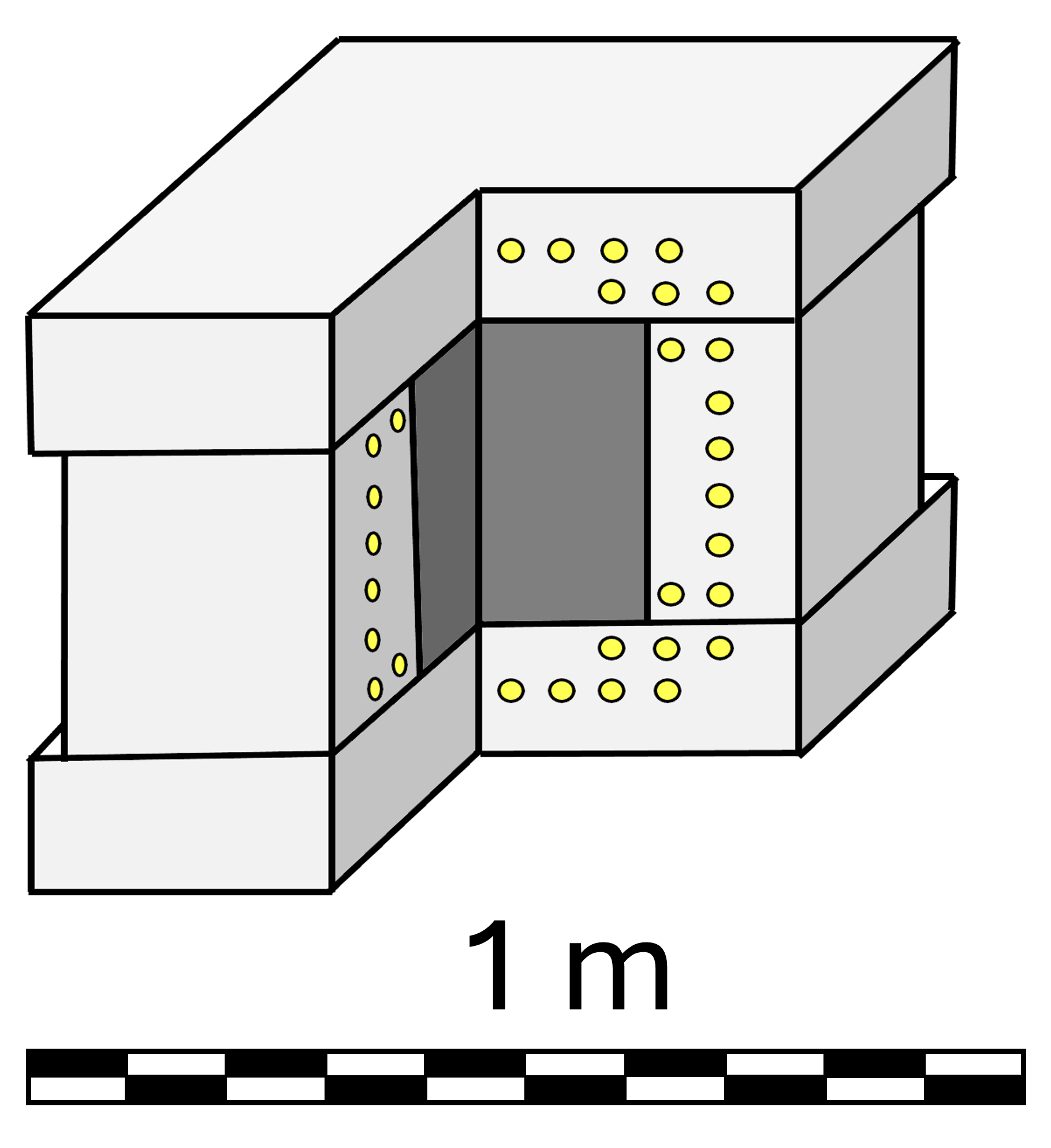
Refer to caption — Figure 1: Schematic representation of the NMDS setup: a 30 cm cube Pb target (dark grey) surrounded by a 15 cm polyethylene moderator (light grey) inlaid with 60 helium-3 neutron counters (yellow).

Each tube was equipped with a preamplifier and connected to a 1400 V high-voltage power supply. The computer-controlled high-voltage units were part of the acquisition system that collected data to a standard PC. The digitiser had a time resolution of 1 $\mu$ s and a 16-bit capacity. When a neutron was detected in any of the tubes, it was assigned to the time-bin #0, and the acquisition remained open for the registration of subsequent neutrons for the next 255 microseconds. After this period, the system was reset to prepare for the next event. The same neutron tube could register multiple events, provided they were spaced by 10 $\mu$ s or more. Assuming a neutron lifetime of 65 $\mu$ s in NMDS, roughly 94% of neutrons from a single event were moderated to the thermal energy range (thermalised) within the 256 $\mu$ s gate. Consequently, a 6% correction was applied during the analysis, reducing the efficiency for detecting multi-neutron events from $23.2\pm 0.2$ %, as determined in experiments using a ²⁵²Cf source, to $22\pm 2$ %. Measurements with the source and Monte Carlo (MC) simulations also confirmed that the detection efficiency is uniform throughout the Pb target volume. In some measurements, the system was enhanced with a $60\times 60$ cm² shield of Geiger counters placed on the top of the setup, detecting the traversing charged particles.

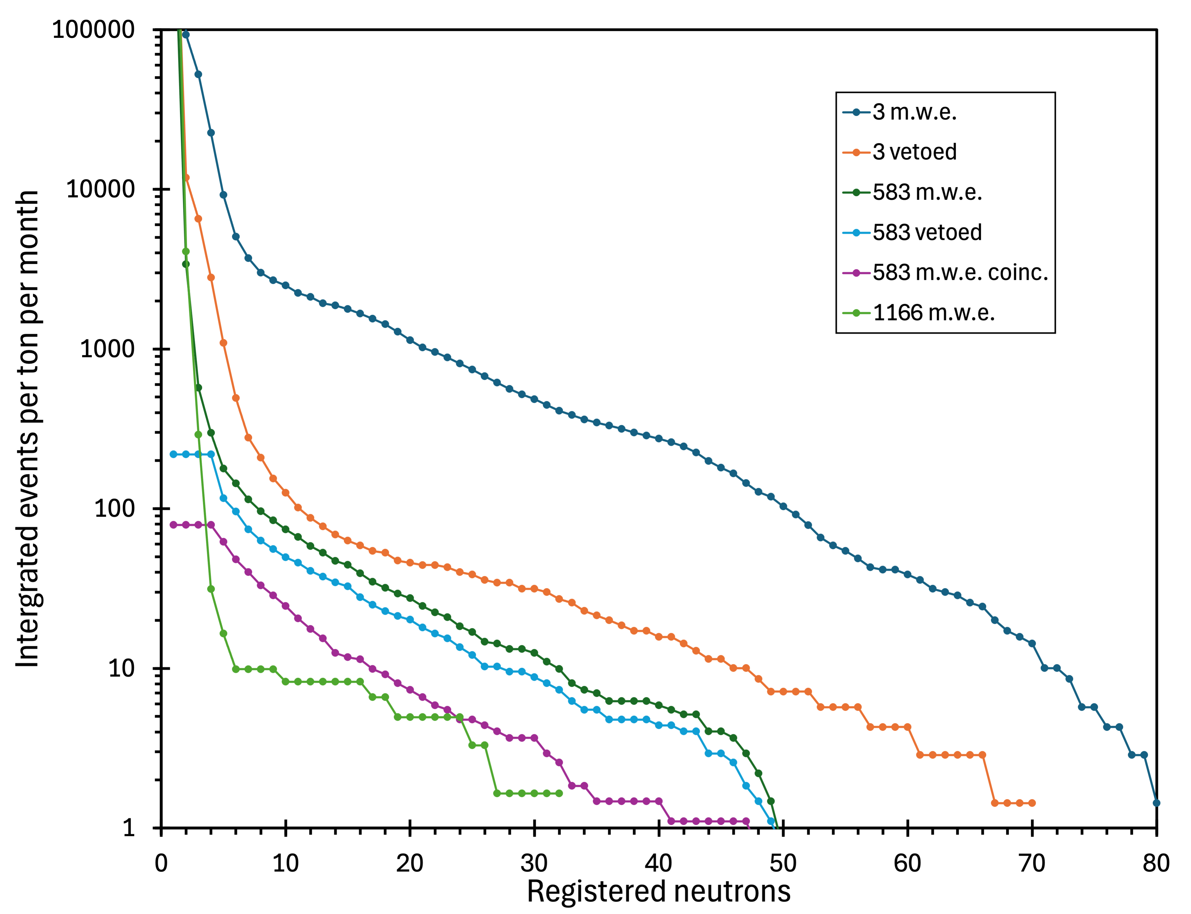
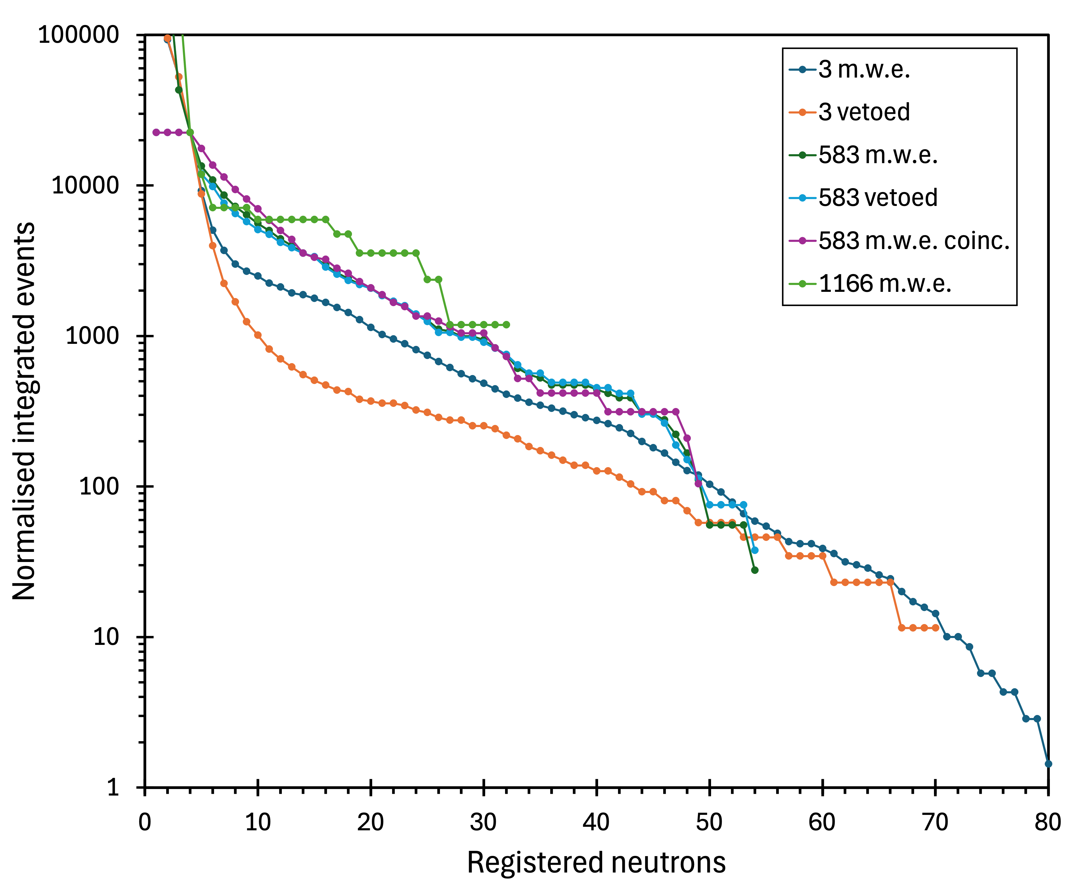
Figure 2 shows all integrated neutron multiplicity spectra measured using the NMDS setup. As the legend indicates, the measured data are derived from six observations at three different depths. The vertical scale (neutron events per ton per month) has been chosen to account for variations in the data acquisition times.

3.1 Measurements at 440 m (1166 m.w.e)

Measurements at the 440 m level in the Pyhäsalmi mine, corresponding to an overburden of 1166 m.w.e., commenced in September 2001. At that time, it was the deepest site accessible to our team. The measurements continued until January 2002, during which 1440 hours of data were acquired (0.612 ton-month). The results are shown in figure 3. Subsequent measurements [17] determined that the muon flux at that depth was 0.014 muons per square metre per second, that is, 1210 muons per square metre per day.

3.2 Measurements at 220 m (583 m.w.e)

In February 2002, NMDS was relocated to a shallower site, offering better infrastructure and accessibility. At the same time, a Geiger counter array was added directly on top of the setup. It consisted of two layers of densely packed Geiger tubes, with an active volume of $60\times 60\times 10$ cm³. Although the coverage of this veto detector was only 1.8 steradians of the total solid angle, it was adequate to provide a sample of coincidence and anti-coincidence (vetoed) neutron multiplicity spectra.

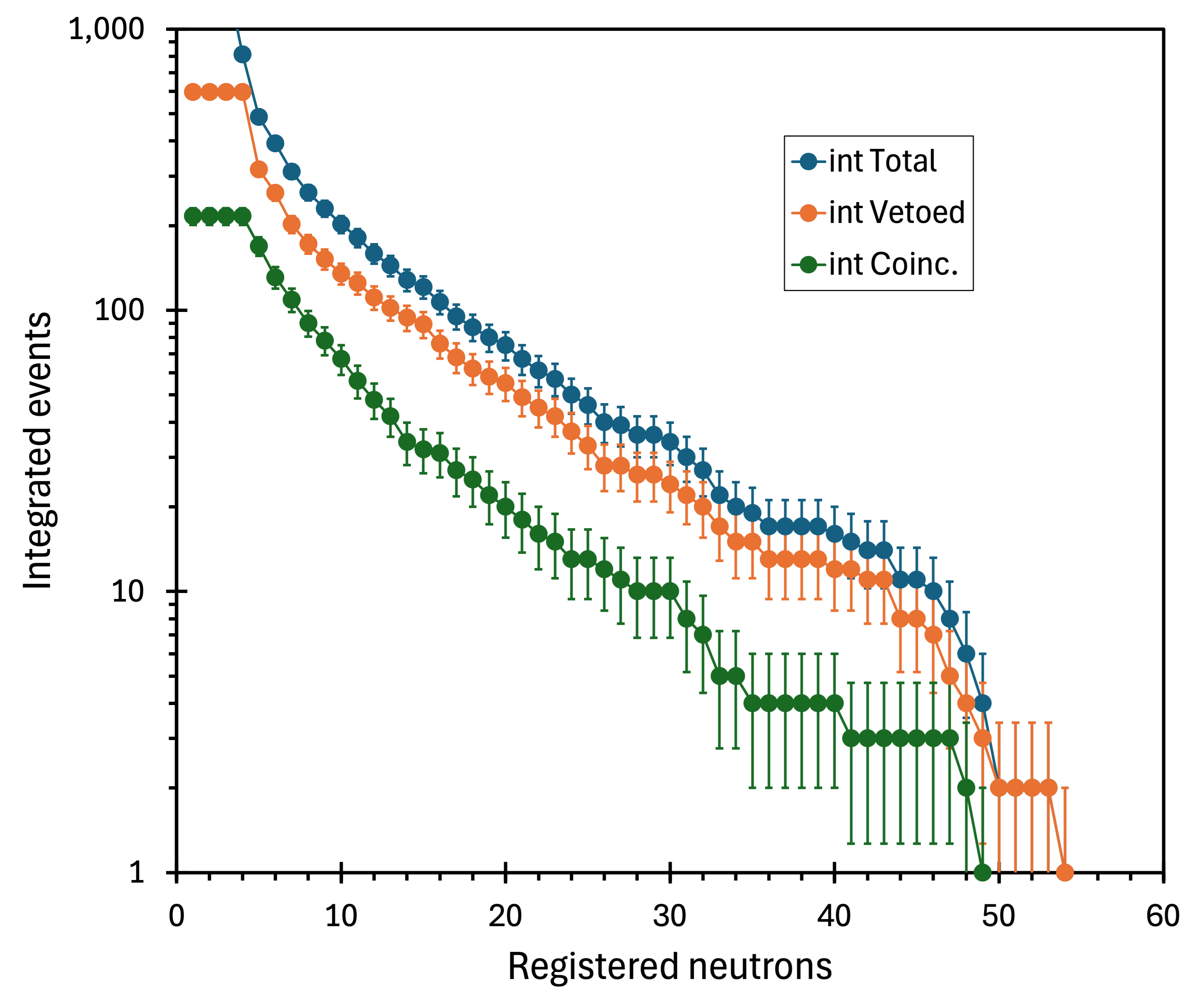
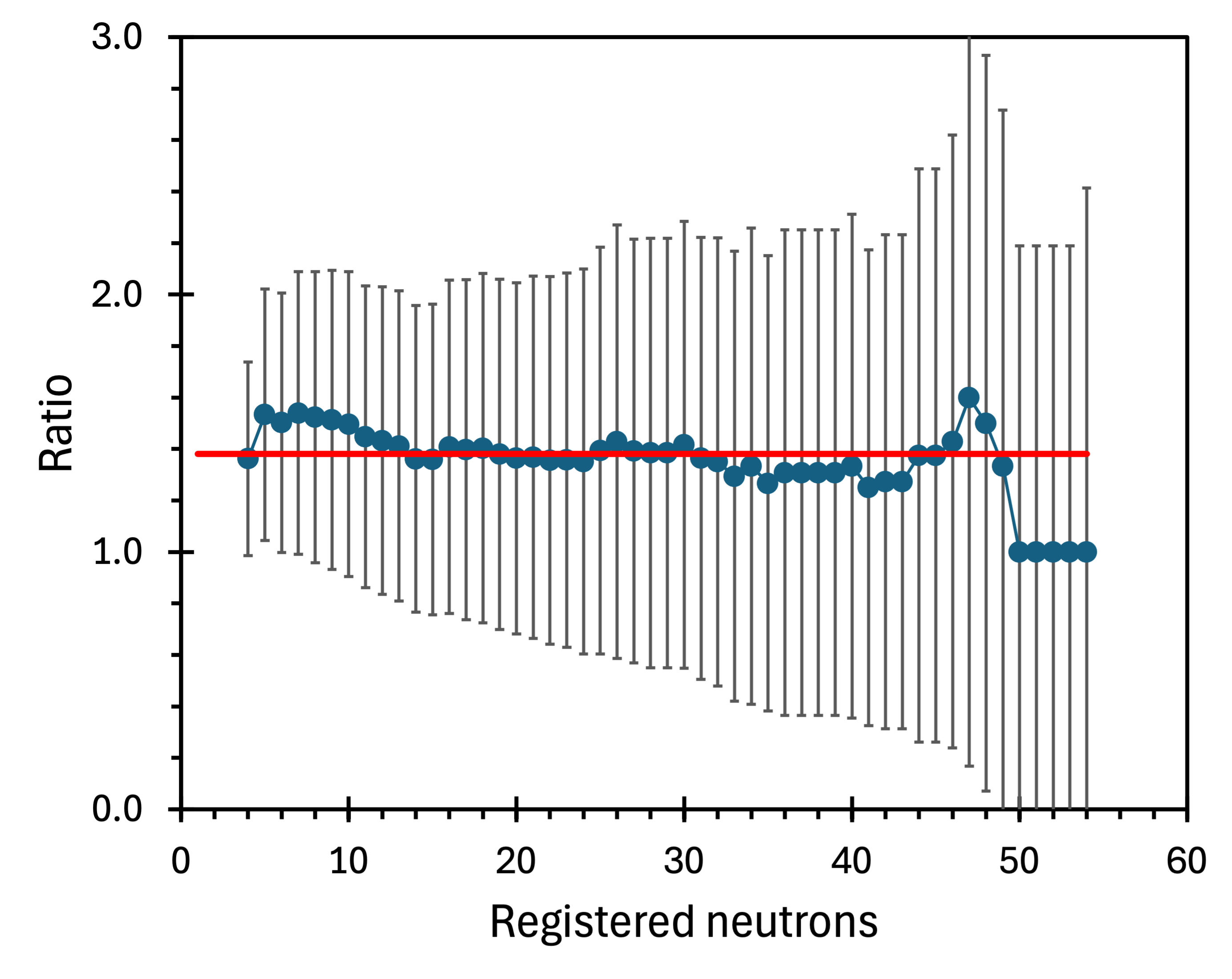
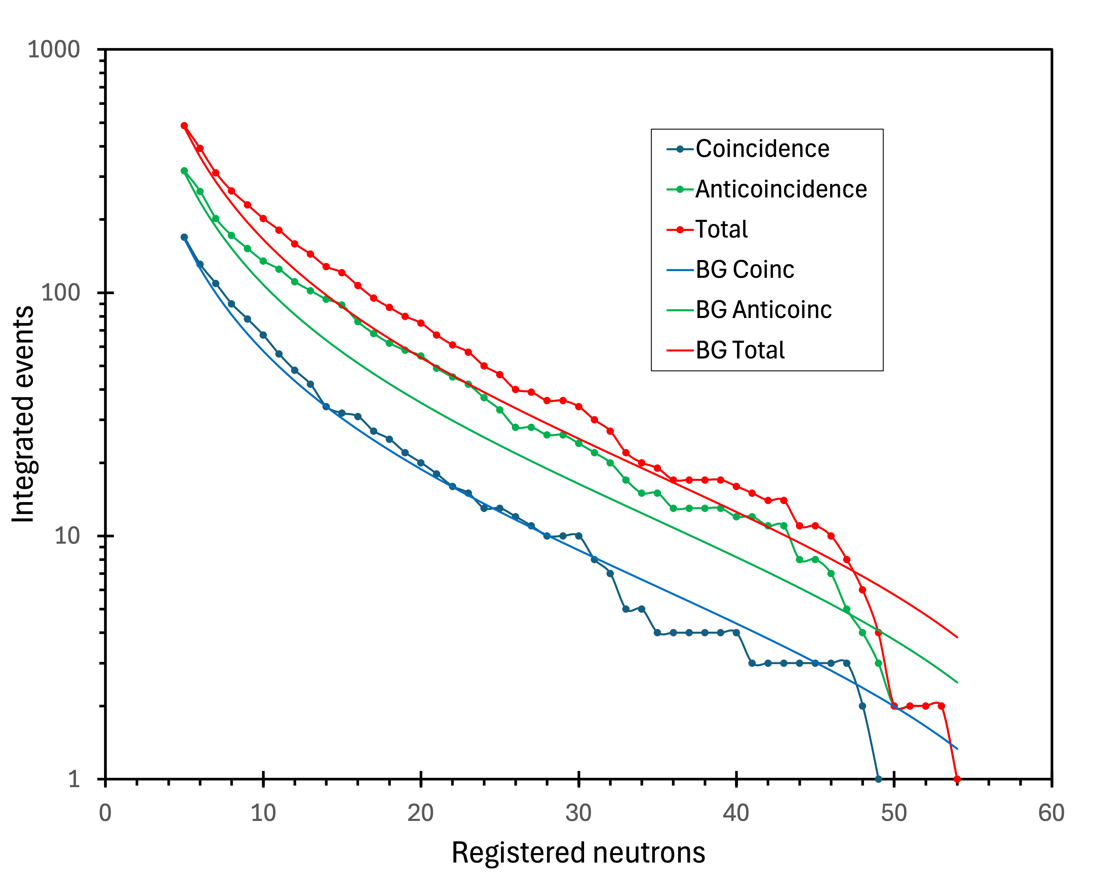
Figure 4 shows the integrated muon multiplicity spectra taken at 583 m.w.e. The top series (blue) represents all the data, the middle (orange points) was taken in anti-coincidence (vetoed) with the Geiger array, and the bottom (green points) was in coincidence with the Geiger array. The spectra exhibit similar shapes, especially the top and the middle. The average ratio between the total and vetoed points is $1.38\pm 0.17$ and remains nearly constant at all neutron multiplicities (figure 5). Spectra collected at 583 m.w.e. represent the best data in this compilation of six measurements conducted over the past two decades, utilising three experimental setups at different sites.

3.3 Measurements in the Lab (3 m.w.e)

The measurements were conducted in room #234 (one floor above the ground level) of the Khlopin Radium Institute building in St. Petersburg. Three metres of water equivalent corresponds to approximately one metre of concrete, accounting for the roofs and ceilings of the floors above. Data were collected for 1668 hours from May to July 2008 using a modified NMDS setup shown in the right panel of figure 6.

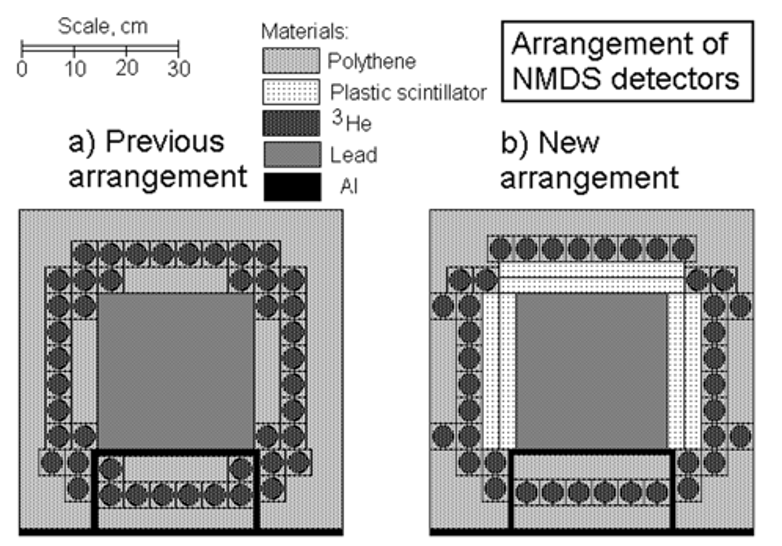
The modification involved adding 18 kg of a plastic scintillator, arranged as five detectors on the four sides and the top of the Pb cube, as illustrated in figure 6. Each detector comprised a sandwich of two scintillator plates measuring $30\times 30\times 2$ cm³. Each plate was coupled with a Hamamatsu R6231-01 PMT. Adding five detectors in direct contact with the target necessitated a slight rearrangement of some of the 60 He-3 neutron counters and the removal of parts of the PE moderator. However, as the scintillator’s moderating properties closely resemble PE’s, the overall change in neutron detection efficiency was minimal. The modified NMDS retained 90% of the original setup’s neutron detection efficiency.

A programmable logic controller processed the amplified and shaped signals from ten PMTs. The acceptance threshold was set at 3 MeV, just below the signal’s amplitude associated with charged particles. To ensure compatibility with the old data format, the coincidence signal from the scintillator shield was added as input #0 among the 60 inputs designated for the neutron detectors. Naturally, some high-energy gamma rays could also generate a trigger. Since neutron detection did not accompany 92.4% of the scintillator triggers, data were recorded only if at least one neutron was present. The collected neutron multiplicity spectra are shown in figure 7.

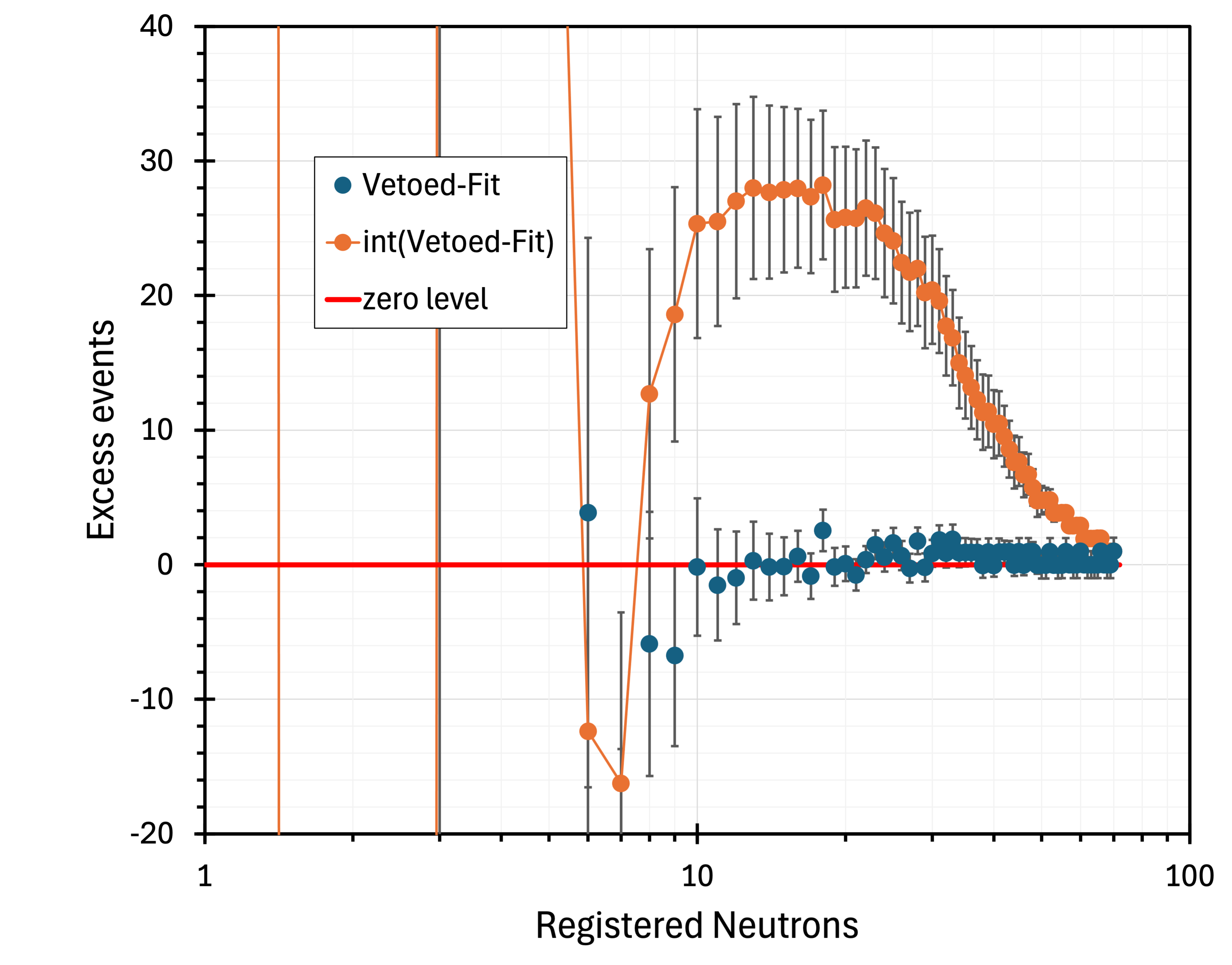
As explained in the Introduction, the instrumentation on the Earth’s surface and at shallow locations is subject not only to muons but also to heavier charged particles originating from CR-induced showers. Therefore, we have searched for anomalies at 3 m.w.e. in the vetoed neutron multiplicity spectrum rather than the total spectrum. Figure 8 shows the excess events (blue points) remaining after subtracting the power-law function fitted to the data with multiplicity $3\leq m\leq 20$ , indicated in figure 7 as a solid red line. The integrated difference is the orange points in figure 8. It reaches a maximum at $m=13$ with $28\pm 7$ integrated excess events. Since the exposure was 0.7089 ton-month, the detected excess corresponds to $40\pm 10$ events per ton per month.

4 Evaluation of NMDS Spectra

4.1 Normalised NMDS Spectra

To search for and emphasise possible trends emerging from the NMDS measurements, we have replotted figure 2 by normalising the spectra at a low neutron multiplicity. Due to the limitations of how the vetoed spectrum at 583 m.w.e. was acquired (with no data for $m<4$ ), the lowest available normalisation point was $m=4$ . However, normalising at a slightly different neutron multiplicity would not fundamentally alter the overall picture. The outcome is illustrated in figure 9. The normalisation appears to have reversed the trend visible in figure 2, where, as expected, the neutron multiplicity spectra progressively weakened with the increase in the overburden and the decline in the muon flux. Normalising the spectra at $m=4$ (figure 9) shows a clear rise in the relative intensity of the mid-multiplicity ( $6<m<46$ ) with the depth. When the registered multiplicity ( $m$ ) is converted to the actual multiplicity ( $M$ ), the range becomes $27<M<209$ . For the conversion, the registered multiplicity ( $m$ ) was divided by the 22% detection efficiency measured with a ²⁵²Cf source and corrected for the fixed 256-microsecond data acquisition time gate, as explained in Section 3.

4.2 Normalised and linearised NMDS Spectra

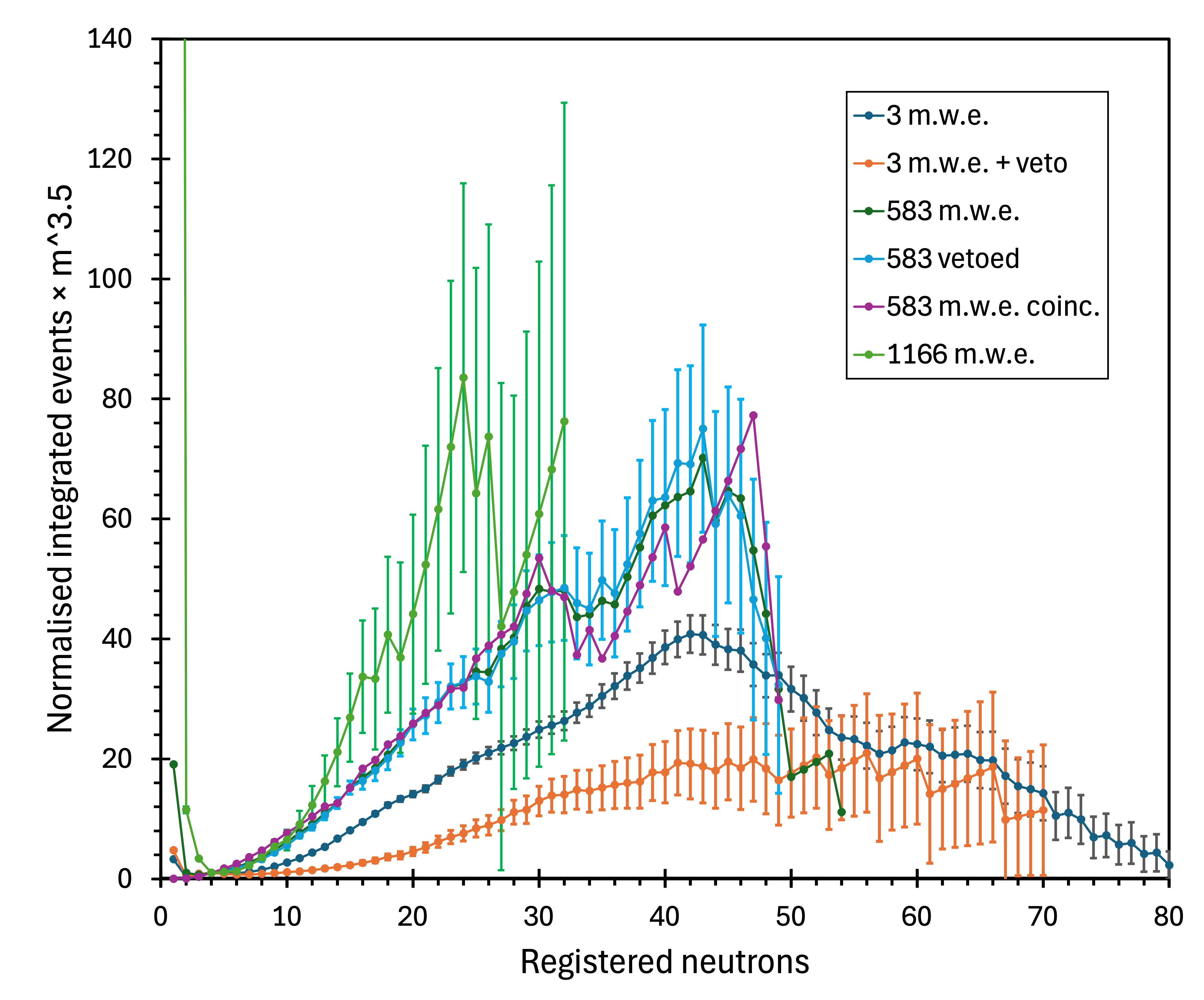
As the number of registered events at any depth decreases by many orders of magnitude between low and high neutron multiplicity values, evaluating linearised plots is a more convenient way to assess spectral shape changes. To do so, the data from figure 9 was multiplied by $m^{3.5}$ (neutron multiplicity to the power of 3.5) and renormalised in figure 10.

4.3 NMDS Monte Carlo Simulations

Significant effort and resources were committed to simulating muon-induced neutron generation in and around the NMDS setup at 583 and 1166 m.w.e. and their subsequent detection in the 60 He-3 counters. These simulations were the focus of a PhD Dissertation defended by Haichuan Cao in May 2023 at the Department of Physics and Astronomy at Purdue University, Indiana, USA [18] and summarised in a paper [3].

The primary outcome of this dissertation is that Geant4 simulations of the registered neutron multiplicity spectra are well-approximated by a two-parameter power-law function $k\times m^{-p}$ , where $k$ and $p$ are the parameters and $m$ is the registered neutron multiplicity. While the simulation accurately determines the slope parameter $p$ , the Geant4-predicted amplitude parameter $k$ is by a factor of two larger than the one fitted to the experimental data. Therefore, for a good agreement, the amplitude must be extracted from the fitting or reduced 50%. It was also concluded that the slope parameters $p$ , measured and simulated, at 583 m.w.e. and 1166 m.w.e. are practically the same. The results for 583 m.w.e. are: $p_{\text{MC}}=2.37\pm 0.01$ and $p_{\text{fit}}=2.36\pm 0.10$ . For 1166 m.w.e., the corresponding values are: $p_{\text{MC}}=2.3\pm 0.01$ and $p_{\text{fit}}=2.50\pm 0.35$ . The amplitude parameters (in thousands) are $k_{\text{MC}}=11.6\pm 0.28$ and $k_{\text{fit}}=5.2\pm 1.2$ for 583 m.w.e., and $k_{\text{MC}}=0.44\pm 0.11$ and $k_{\text{fit}}=0.19\pm 0.17$ for 1166 m.w.e. The quoted errors are statistical only.

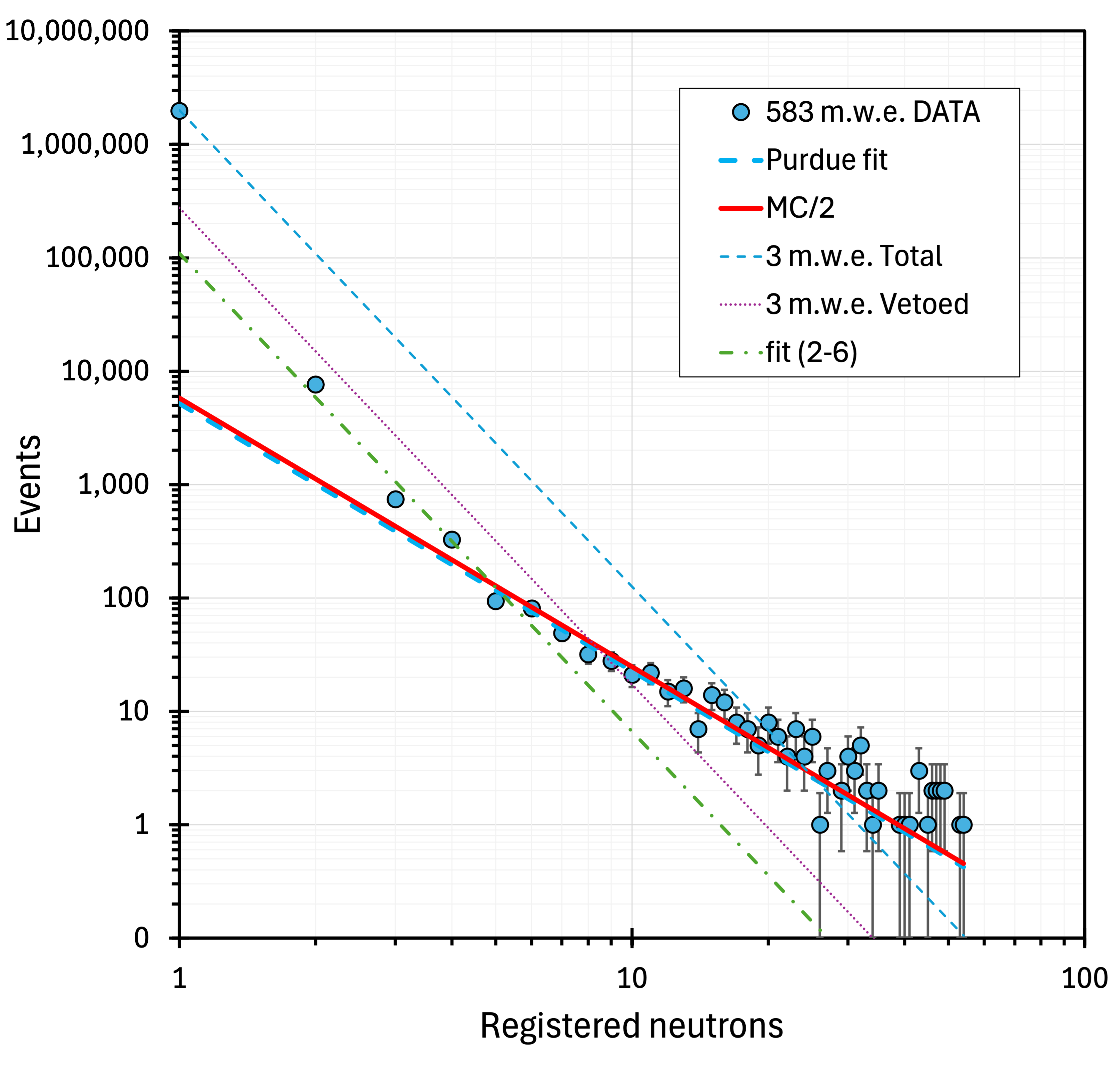
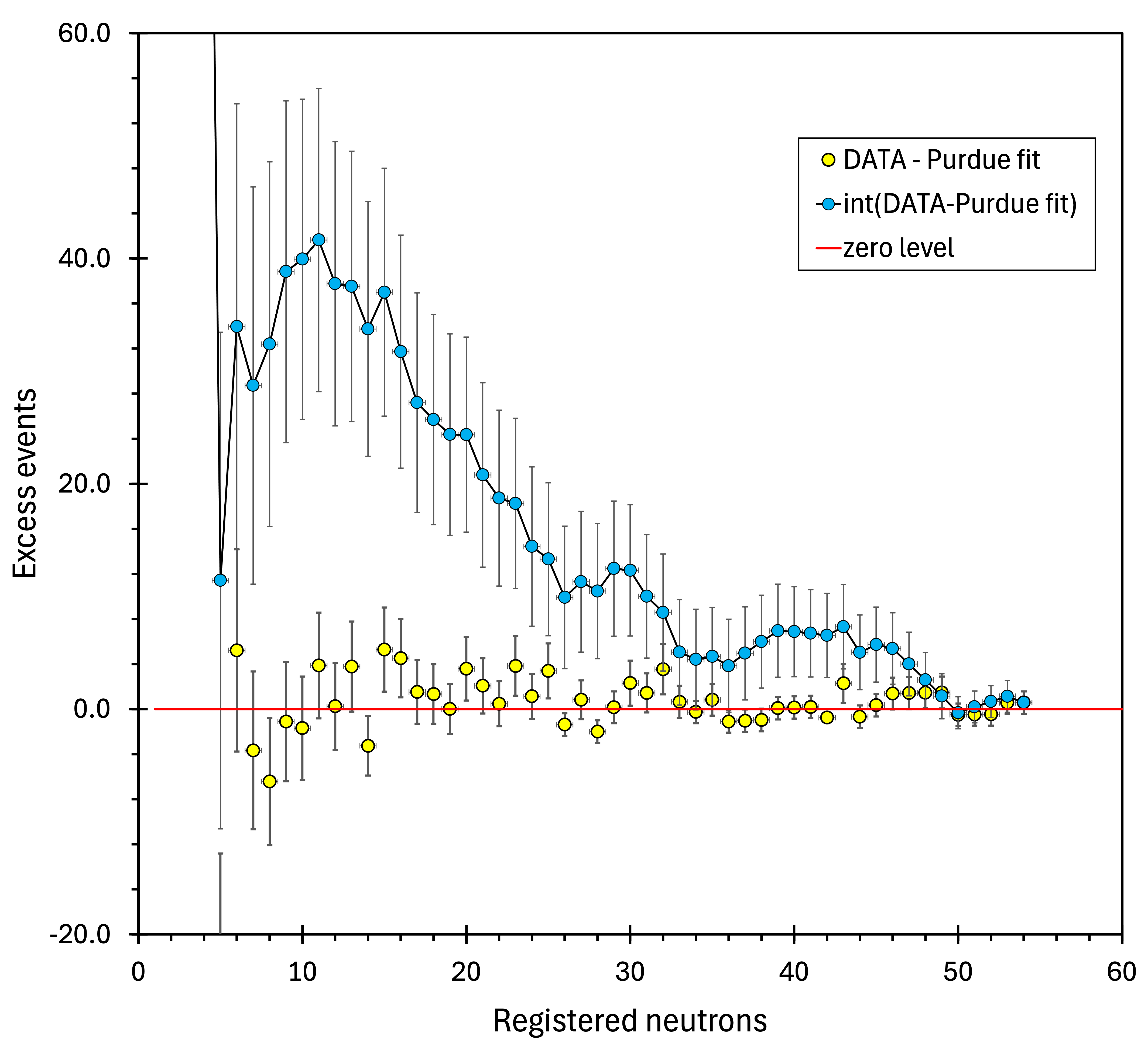
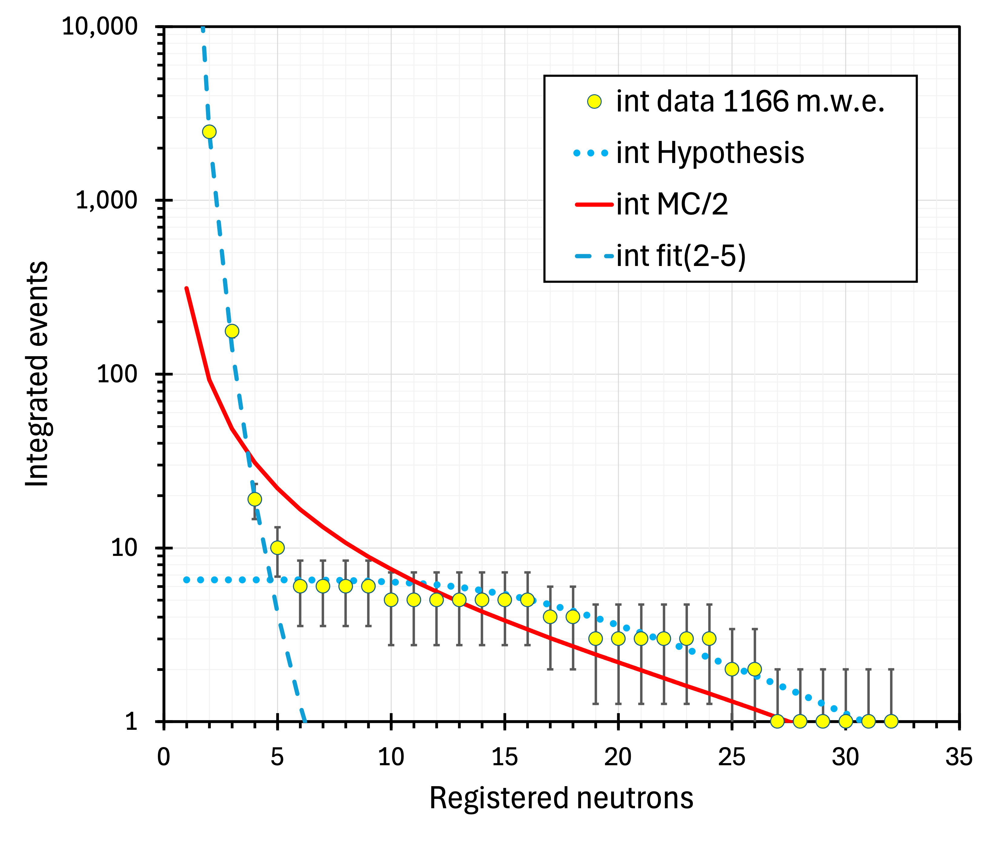
Figure 11 shows the NMDS total spectrum measured at 583 m.w.e. (points with error bars). The thick blue dashed line is the Purdue power-law fit ( $p=2.36$ , $k=5200$ ). It practically overlaps with the fit to the MC outcome (solid red line). We treat the fitted line as a reliable parametrisation of the muon-induced neutron contribution and subtract it from the measured spectrum. If anomalies are present, they would manifest themselves as statistically significant bumps in the subtracted spectrum. Otherwise, the resulting points would be evenly distributed above and below the zero line. Integrating the background-subtracted spectra may further enhance the visibility and strengthen the evidence for anomalies. In figure 12, the fitted function ( $p=2.36$ , $k=5200$ ) was subtracted from the data (yellow points). The blue points represent the integrated difference between the data and the fit. Although the yellow points oscillate around zero, as they should, the integrated values (blue points) cumulate an excess of events for multiplicities $5<m<50$ , peaking at $m\sim 11$ with $42\pm 14$ events, i.e., $15\pm 5$ events per ton-month, a clear three-sigma effect.

To incorporate the fitted function and the MC-simulated trends into figure 10, integrated and normalised values of these power-law dependencies are needed. Integrating data is noncontroversial. Integration ends with the last channel containing data. However, it is not obvious how to deal with power-law functions. The problem is illustrated in figure 13. Integrated experimental data points are shown as dots with error bars. The top line is the outcome of the integration of the Purdue fit up to multiplicity 200; the middle, up to $m=64$ (ten channels above the highest recorded event), and the bottom, up to $m=54$ (the highest recorded event). None of the trends fully represent the measured data. Still, the middle red curve gives the best match, and it is used (for visualisation only) in figure 14. Otherwise, the integrated power-law functions are not needed for the analysis. The quantitative values are extracted by integrating the difference between the measured data and the power-law function; therefore, the integration range ambiguity is resolved.

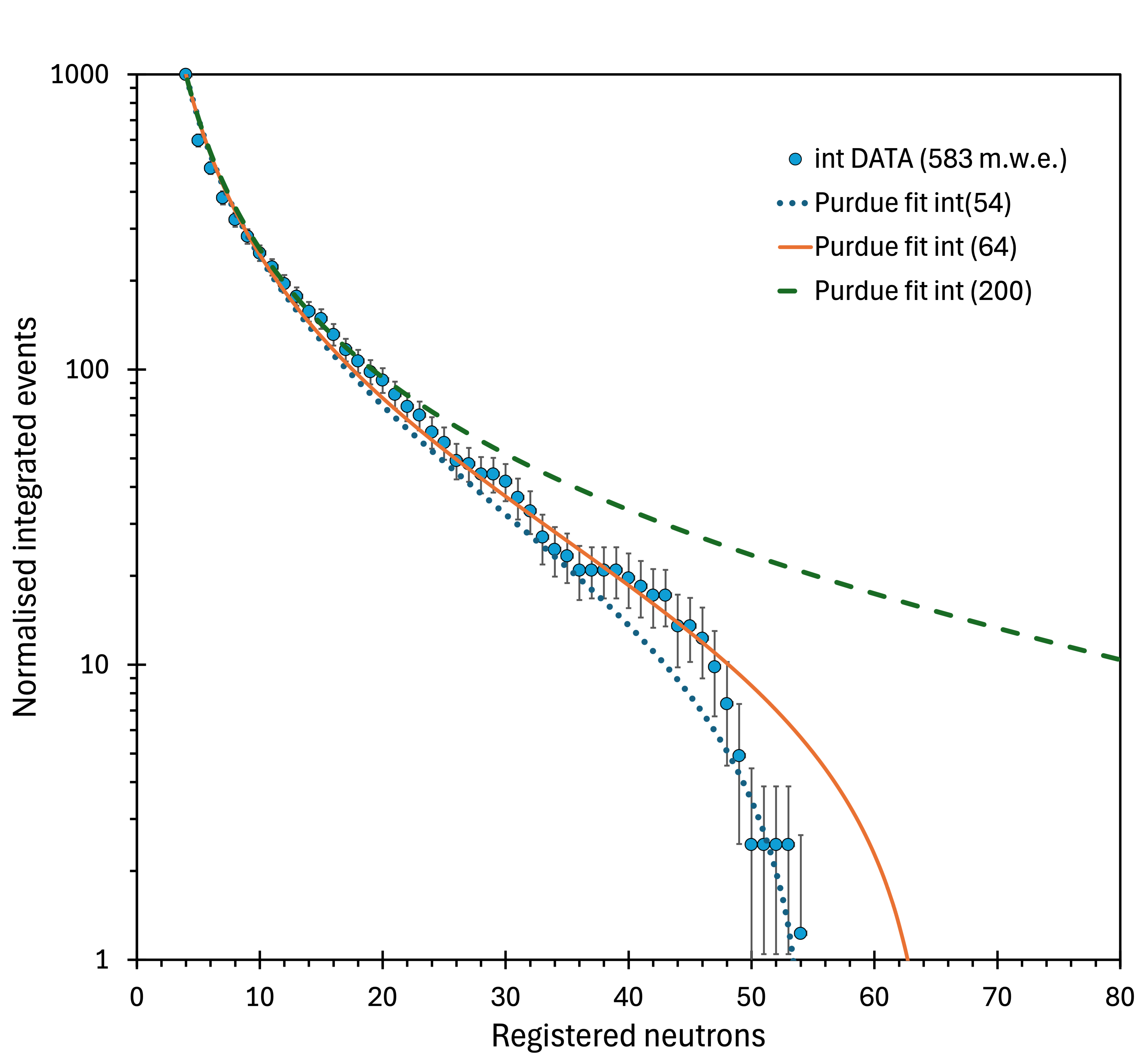
Figure 14 compares the measured values at 3 m.w.e (red points), 583 m.w.e. (orange points) and at 1166 m.w.e (green points) with the Purdue fit to 583 m.w.e. data (green solid line) and MC predictions for 1166 m.w.e. depth (black solid line) and 583 m.w.e. (black dashed line). The red dotted lines in figure 14 represent the shape of the 3 m.w.e. data (read points) multiplied by 1.7 and 3.0, to match the measured spectra at 583 and 1166 m.w.e., respectively. As the slope parameters of the Purdue fit ( $p=2.36$ ) and the MC prediction ( $p=2.37$ ) are similar, and both were integrated up to $m=64$ , the two lines are very close in figure 14 and follow the 583 m.w.e. data trend up to $m=47$ . However, the measured 1166 m.w.e. values (green points) deviate noticeably from the MC-expected trend (black solid line) integrated up to $m=74$ . The 1166 m.w.e. data ends abruptly at $m=32$ due to low statistics (figure 3). The acquisition time should have been significantly longer to cover higher multiplicities.

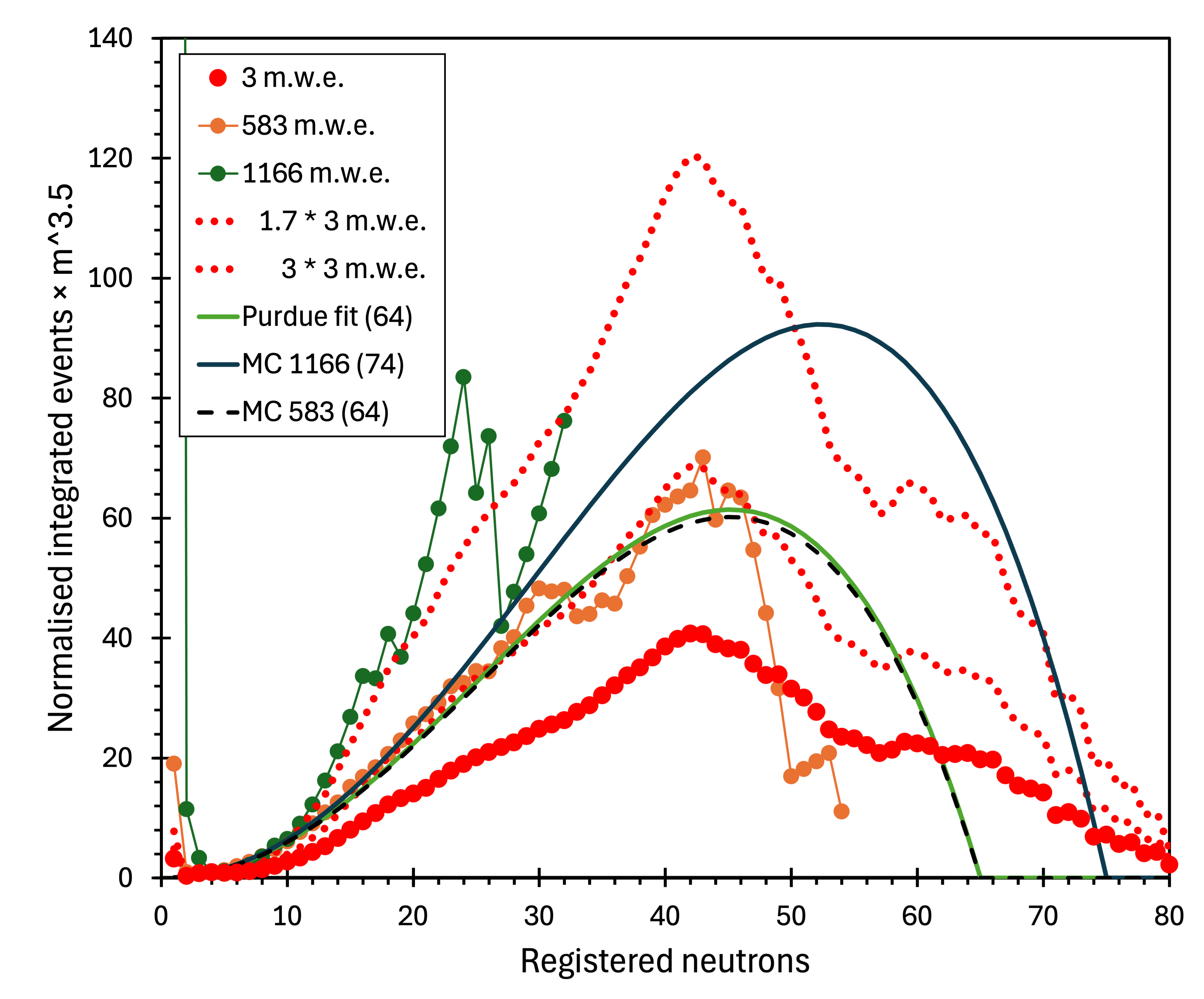
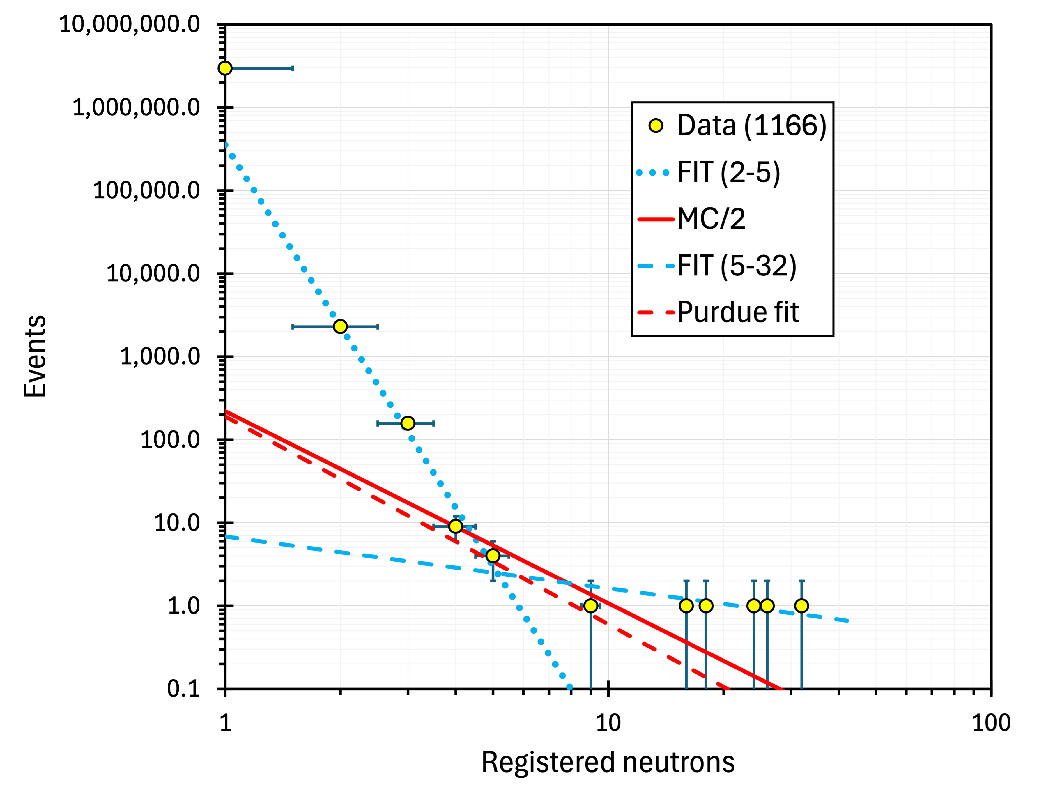
Another feature of the 1166 m.w.e. spectrum (figure 3) is the discrepancy between the Purdue fit, the MC, and the data. Two different power-law fits are needed to describe the measured values: for $2\leq m\leq 5$ (blue dotted line) and $5\leq m\leq 32$ (blue dashed line). The former is considerably steeper ( $p=7.26$ ), and the latter is significantly flatter ( $p=0.623$ ) than the MC prediction ( $p=2.31$ ). The inadequacy of the MC prediction for 1166 m.w.e. is also visible in figure 14.

4.4 Coincidence and Anticoincidence Neutron Multiplicity Spectra

In addition to the total spectrum, coincidence and anticoincidence (vetoed) spectra were also recorded at 583 m.w.e. The Purdue MC study evaluated the power-law parameters only for the Total neutron multiplicity spectrum. While the shape parameter stays the same ( $p=2.36$ ), determining the amplitude parameters for the coincidence and anticoincidence spectra was needed. Figure 15 illustrates our $k$ -finding procedure. As the integrated total spectrum and its power-law background cross at $m=5$ , we adjusted the $k$ parameters of the coincidence and anticoincidence muon-induced background spectra to have the same property. The resulting parameters are $k=1808$ for the former and $k=3392$ for the latter.

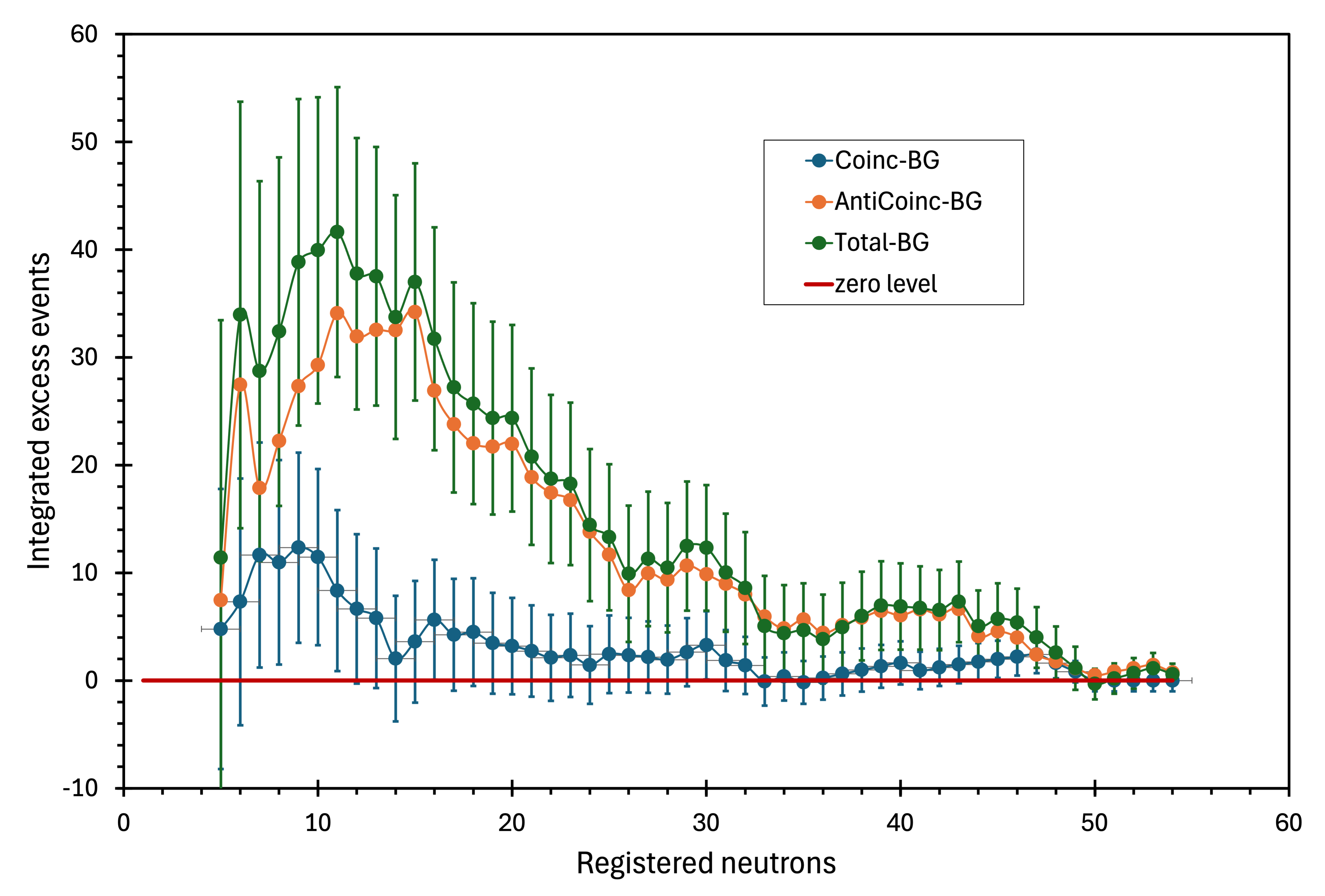
If the anomalous excess in neutron multiplicity is genuine and unrelated to the muon flux, one would expect a diminished effect for the spectrum recorded in coincidence with the muon-triggered Geiger array. At the same time, the anti-coincidence spectrum would retain the excess and be less contaminated with muon-induced neutrons at the cost of somewhat lower statistics. This is indeed the case, as shown in figure 16. While the excess in the total spectrum is $42\pm 14$ events and $34\pm 11$ events in the anticoincidence spectrum, there are at most $12\pm 11$ excess events in the coincidence spectrum. These values correspond to $15\pm 5$ , $13\pm 4$ , and $4.3\pm 3.9$ events per ton per month, respectively.

4.5 Smoothed Neutron Multiplicity Spectra

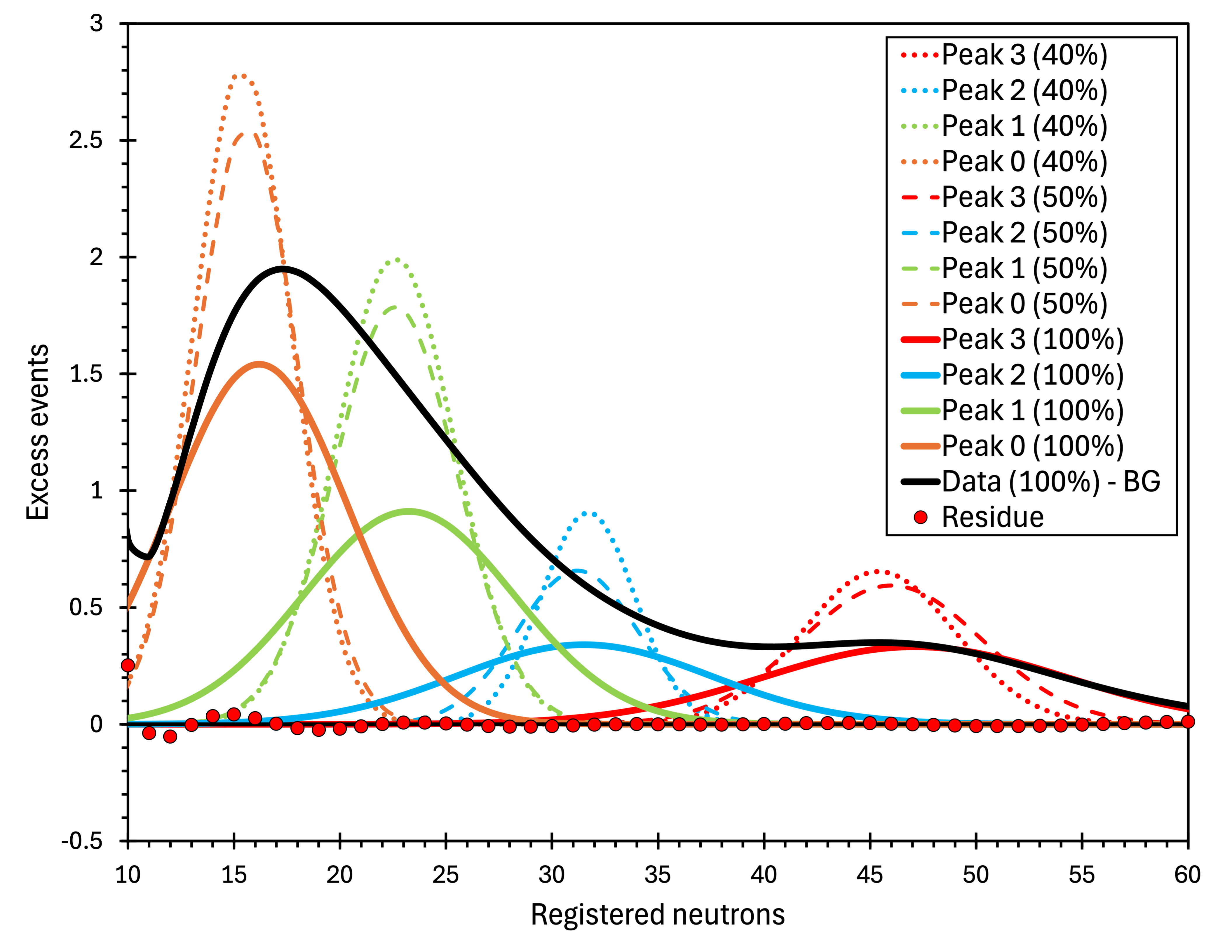
As explained in Section 2.2 2.2, smoothing is a useful tool for addressing low statistics. Figure 17 displays the smoothed, non-integrated, background-subtracted neutron multiplicity spectrum obtained in anticoincidence with the Geiger array at 583 m.w.e. Regarding muon contamination, it is the cleanest high-statistics data sample we have. The smoothing was done with $\sigma=0.5\sqrt{m}$ . The outcome has a structure resembling four Gaussian peaks. While the existence of the excess events in the range of $10<m<54$ is evident, the available statistics do not warrant a conclusive statement on the shape and structure of the excess events. Indeed, smoothing procedures tend to induce slight undulations. To check if this is the case, we have repeated smoothing with $\sigma=40,50,and100\%\sqrt{m}$ and fitted Gaussian peaks to the resulting spectra. If the peaks were artefacts, their number, positions, and areas would significantly change or disappear with intensified smoothing. If not, they may be real. All four peaks survived the test. Their position stayed within one multiplicity channel, and the peak areas remained within 2% for peaks 0, 2, and 3 and 19% for peak 1. Figure 18 shows the four peaks fitted to the spectra smoothed with $\sigma=40\%\sqrt{m}$ (dotted lines), $\sigma=50\%\sqrt{m}$ (dashed lines), and $\sigma=100\%\sqrt{m}$ (solid lines). The black solid line is the $\sigma=100\%\sqrt{m}$ smoothed background-subtracted spectrum, and the red points are the fitting residue. Since the residue is minimal, the description with four peaks matches the data well. The parameters of the four peaks, obtained by fitting to the $\sigma=100\%\sqrt{m}$ smoothed spectrum, are in table 1. The peaks are also visible in the Total 583 m.w.e. spectrum.

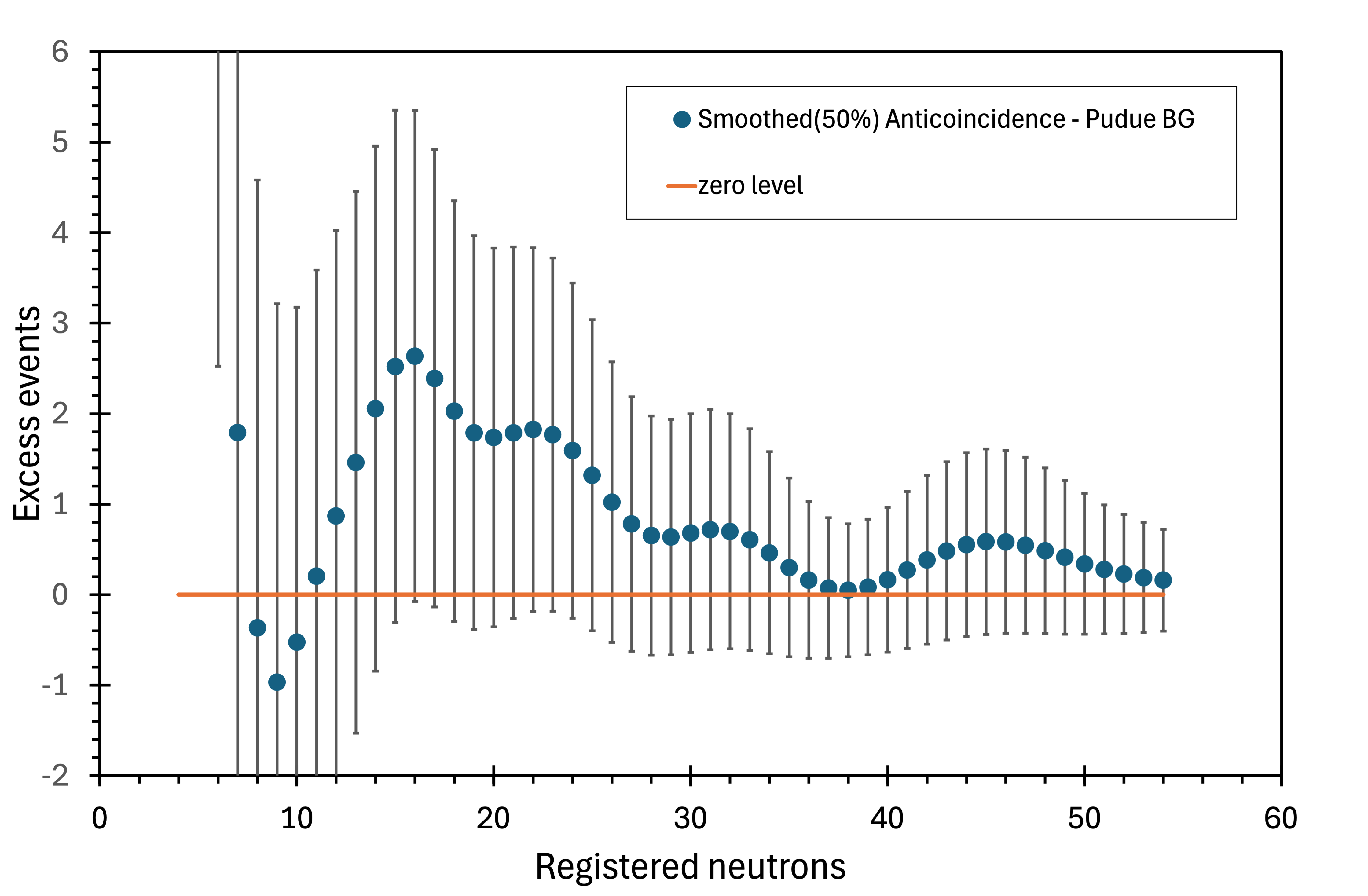
Since the four peaks retain their positions and areas under progressive smoothing, their width ( $\sigma$ ) parameters positively correlate with peak positions and are greater or equal to the square root of their position, as expected from the statistics and our neutron detection efficiency, we treat the fitted peaks as a plausible hypothesis to be verified by future measurements. If the energy spectrum of the excess neutrons resembles that of ²⁵²Cf, the detection efficiency should be $\sim 22\pm 2$ %. We can estimate the actual neutron multiplicities of the suspected anomalies using this value. The results are listed in table 1.

	Peak 0	Peak 1	Peak 2	Peak 3
Position (m)	16.2	23.3	31.5	47.1
Sigma	4.2	5.0	6.0	7.2
$\sqrt{m}$	4.0	4.8	5.6	6.9
Area (events)	16.1	11.4	5.1	6.0
Fraction of total excess (%)	$\sim$ 41.8	$\sim$ 29.5	$\sim$ 13.3	$\sim$ 15.4
Actual neutron multiplicity (M)	$74\pm 7$	$106\pm 11$	$143\pm 14$	$214\pm 21$

Table 1: Parameters of Gaussian peaks describing event excess registered in the Anticoincidence (vetoed) spectrum at 583 m.w.e. and smoothed with

\sigma=\sqrt{m}

5 NCBJ Setup and Measurements

NCBJ is a Polish acronym for the National Centre for Nuclear Research – one of the largest scientific institutes in Central Europe. This name was chosen for the setup because it was first used at the now-decommissioned underground site of the NCBJ Cosmic Ray Laboratory in Łódź, Poland. The main element of the setup, schematically depicted in figure 19, was an array of fourteen proportional counters [19], filled with He-3 at four atmospheres and surrounded by a PE moderator forming a $75\times 6.4\times 55$ cm³ box of an approximate weight of 25 kg. The helium counters, produced by ZdAJ, Poland [20], are 2.54 cm (1”) in diameter and 50 cm in length. Previously, they have been used for neutron background measurements in several European underground laboratories [21, 22, 23] as part of the ILIAS and BSUIN projects [24].

The setup was equipped with a custom-made Neutron Data AcQuisition (NDAQ) system [25]. Each detector had a built-in preamplifier and a digitiser sampling the signal for 0.3 ms before and 1.7 ms after the trigger. The trigger was generated whenever any detector registered a valid signal. The sampling time width was sufficient to account for variations in neutron thermalisation. The sampling step and the software allow the detection of multiple neutrons in the same counter if they are spaced by more than $2-3$ $\mu$ s. Data-taking was controlled remotely. The extraction of neutron multiplicity from the digitised waveforms is described in [26]. NDAQ is considerably more advanced than the NMDS data acquisition system. At the same time, the number of neutron detectors (14 vs. 60) and, consequently, the detection efficiency ( $\sim$ 8% vs. $\sim$ 22%) are considerably smaller. Also, no in-depth MC simulations of the NCBJ performance and spectra were completed. However, we have collected a background neutron multiplicity spectrum (without a target) and one reference spectrum using a copper (Cu) target in addition to the Pb target.

5.1 Measurements at 40 and 210 m.w.e.

The measurement at the NCBJ Cosmic Ray Laboratory in Łódź, Poland, lasted 264.4 hours. The lab was $\sim$ 13 m underground, corresponding to an overburden of 40 m.w.e. The spectra, recorded in 2010, were first presented in [27] and are shown in figure 20 as the lower data series (dark blue points). The experiment aimed to determine particle cascades’ role in generating large neutron multiplicities. Indeed, the largest recorded multiplicity was $m=45$ . It was proposed that the most likely mechanism of neutron generation is due to interactions of large particle cascades in lead. However, the experiment was intended as a pilot measurement only. Moving on would require a reliable muon tracking system working in delayed coincidence mode with neutron detection. For instance, by integrating neutron detectors with the EMMA experiment [28], located at 210 m.w.e. in the Pyhäsalmi mine [29] in Finland.

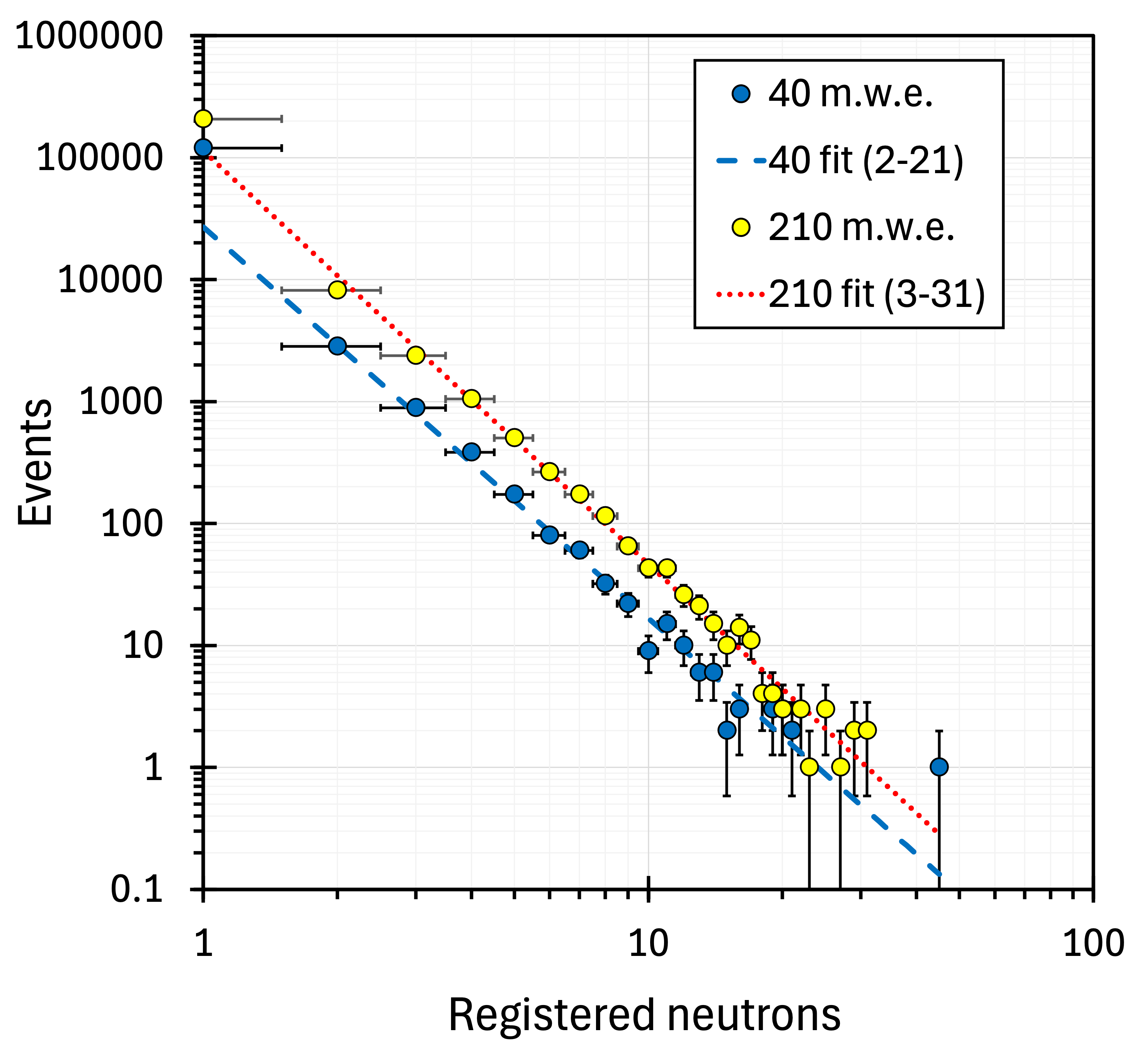
The NCBJ setup was finally relocated to the Pyhäsalmi mine in November 2019. Three measurements were completed at the 210 m.w.e. level before the unavoidable decommissioning of that underground site in November 2022: 344.5 days run with a 565 kg Pb target (a 6.511 ton-month exposure), 200.4 days run without a target, and 259.1 days run with a 448 kg Cu target (a 3.870 ton-month exposure). Unfortunately, strict COVID-19 mobility restrictions, the defunding of the EMMA project, and the closing of the NCBJ Cosmic Ray Laboratory prevented us from incorporating the muon tracking into neutron measurements. Therefore, the presented analysis relies exclusively on neutron data. The Pb neutron multiplicity spectrum collected at 210 m.w.e. is shown in figure 20 (yellow points).

6 Evaluation of the NCBJ Spectra

Analysis procedures developed for NMDS data were also applied to NCBJ spectra. Figure 21 is the NCBJ analogue of figure 10. It shows the integrated 210 and 40 m.w.e. data points linearised by the multiplication by $m^{3.5}$ and normalised at $m=2$ . As the error bars for both data series are similar, for clarity, in figure 21, they were plotted only for the 210 m.w.e. data points.

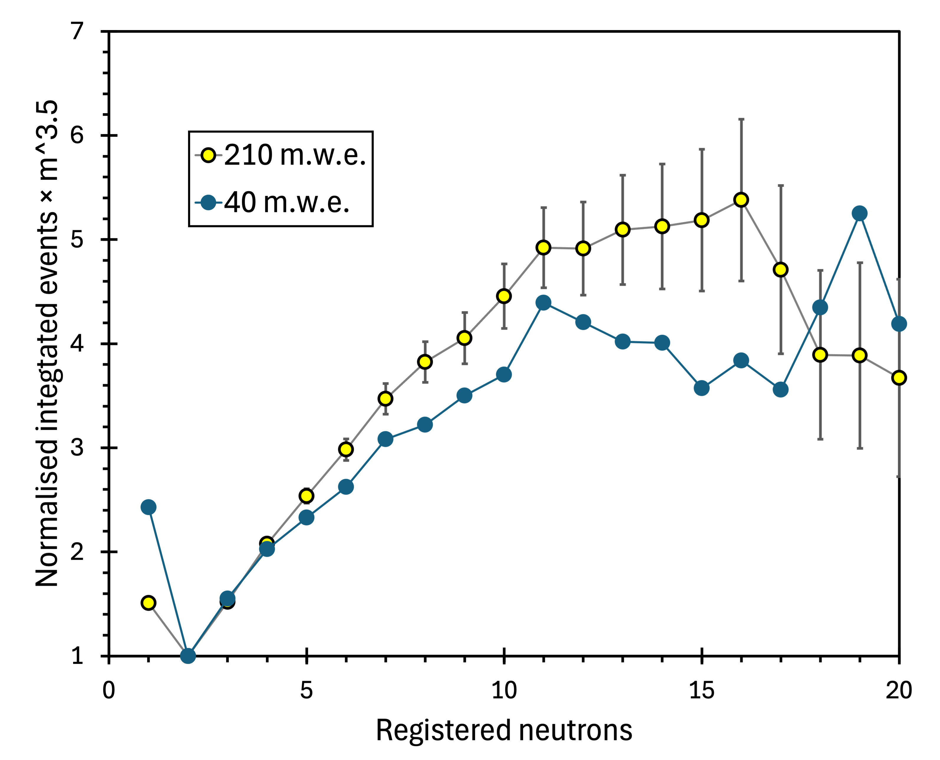
The NMDS analysis indicated (figure 10) a possible excess for multiplicities between the normalisation point and $m\sim 50$ . If the NCBJ setup detected the same phenomenon and, accounting for the $2\frac{3}{4}$ times smaller neutron detection efficiency, there should be a separation between the 210 and 40 m.w.e. data points for multiplicities ranging from the normalisation point up to $m=18$ . It is indeed the case. Furthermore, as suggested by the data shown in figure 10, the points from a deeper location bulge more in figure 21.

6.1 Pb neutron spectrum at 40 m.w.e.

The 40 m.w.e. measurement at the NCBJ Cosmic Ray Laboratory in Łódź was the shortest of all experiments evaluated in this paper. Although it lasted only 11 days, it provided a valuable reference for the 210 m.w.e. spectra. Nevertheless, the data shown in figure 20 was insufficient for a conclusive outcome. The integrated, background-subtracted spectrum yielded $7.6\pm 21$ excess events, i.e., $37\pm 101$ events per ton-month.

6.2 Pb neutron spectrum at 210 m.w.e.

As already mentioned above, no in-depth simulation results exist for the NCBJ setup at 210 m.w.e. However, one of the conclusions of Purdue MC studies [3] was that a power-law fit adequately approximates the muon-induced neutron multiplicity spectrum. Therefore, one can attempt to background-subtract neutron spectra with such a fit. The fit, shown in figure 20, used data points $3\leq m\leq 31$ . The integrated excess above the fitted power-law background is shown in figure 22. It reaches a maximum at $m=4$ , but at lower multiplicities, it fluctuates between large negative and positive numbers. Therefore, we terminate integration at $m=5$ with $75\pm 36$ events to avoid possible contamination at $m=4$ . These $75\pm 36$ events correspond to $12\pm 6$ events per ton-month.

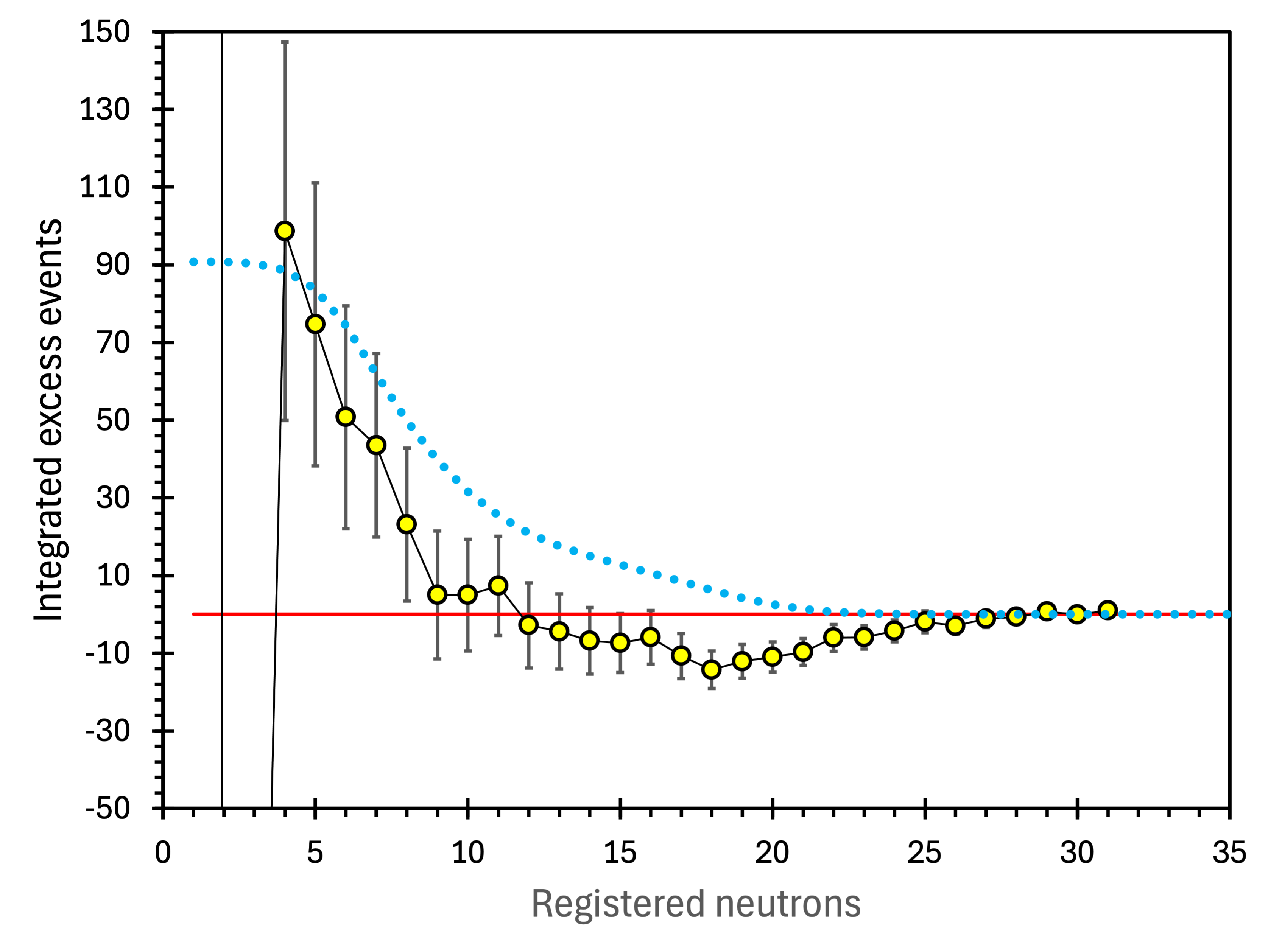
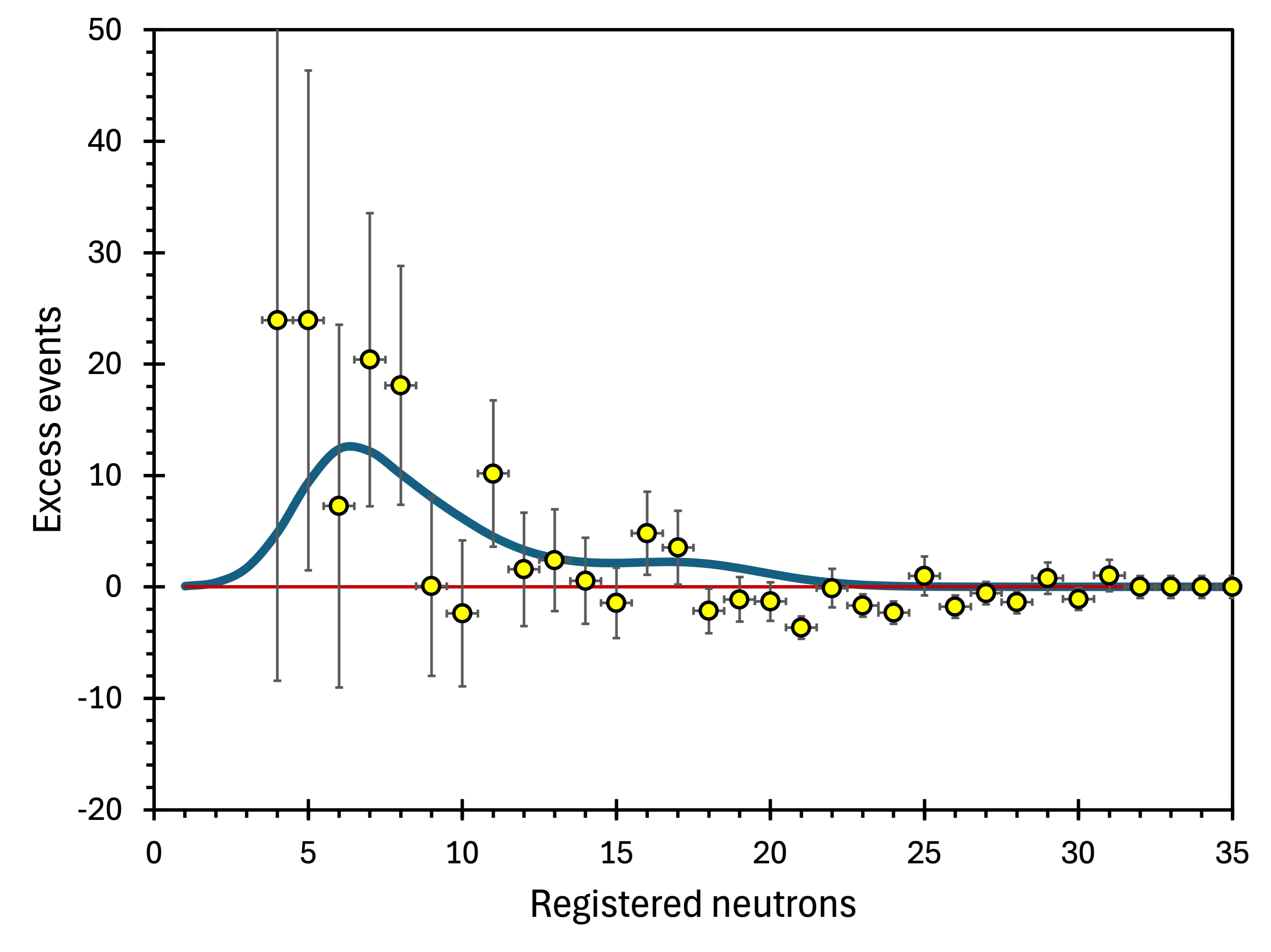
The next step is to evaluate the shape of the excess spectrum. The blue line in figure 23 is the four-peak prediction deduced from the NMDS spectrum at 583 m.w.e. and superimposed on the NCBJ excess events at 210 m.w.e. (points with error bars). The position and sigma parameters of the Gaussian peaks taken from table 1 were reduced $2\frac{3}{4}$ times to adjust for the difference in neutron detection efficiencies. The areas from table 1 were multiplied by 2.36 – the exposure ratio of 6.5107 ton-month vs. 2.7642 ton-month. While the data are insufficient to confirm shape overlap, there is an apparent similarity between the two. It is also visible in figure 22, where the shape of the integrated peaks (blue dotted line) is compared with the integrated excess events at 210 m.w.e. (points with error bars).

6.3 Cu neutron spectrum at 210 m.w.e.

The measurements with the NCBJ setup and a 448 kg Cu target took place between August 2021 and November 2022. The total exposure was 3.870 ton-months. Fifty standard-size ( $20\times 10\times 5$ cm³) Cu bricks were replaced by fifty Pb bricks. Otherwise, the setup’s configuration was not changed. The same analysis procedures were applied to the Cu neutron multiplicity spectrum as previously to the Pb spectrum. The resulting excess spectrum is shown in figure 24.

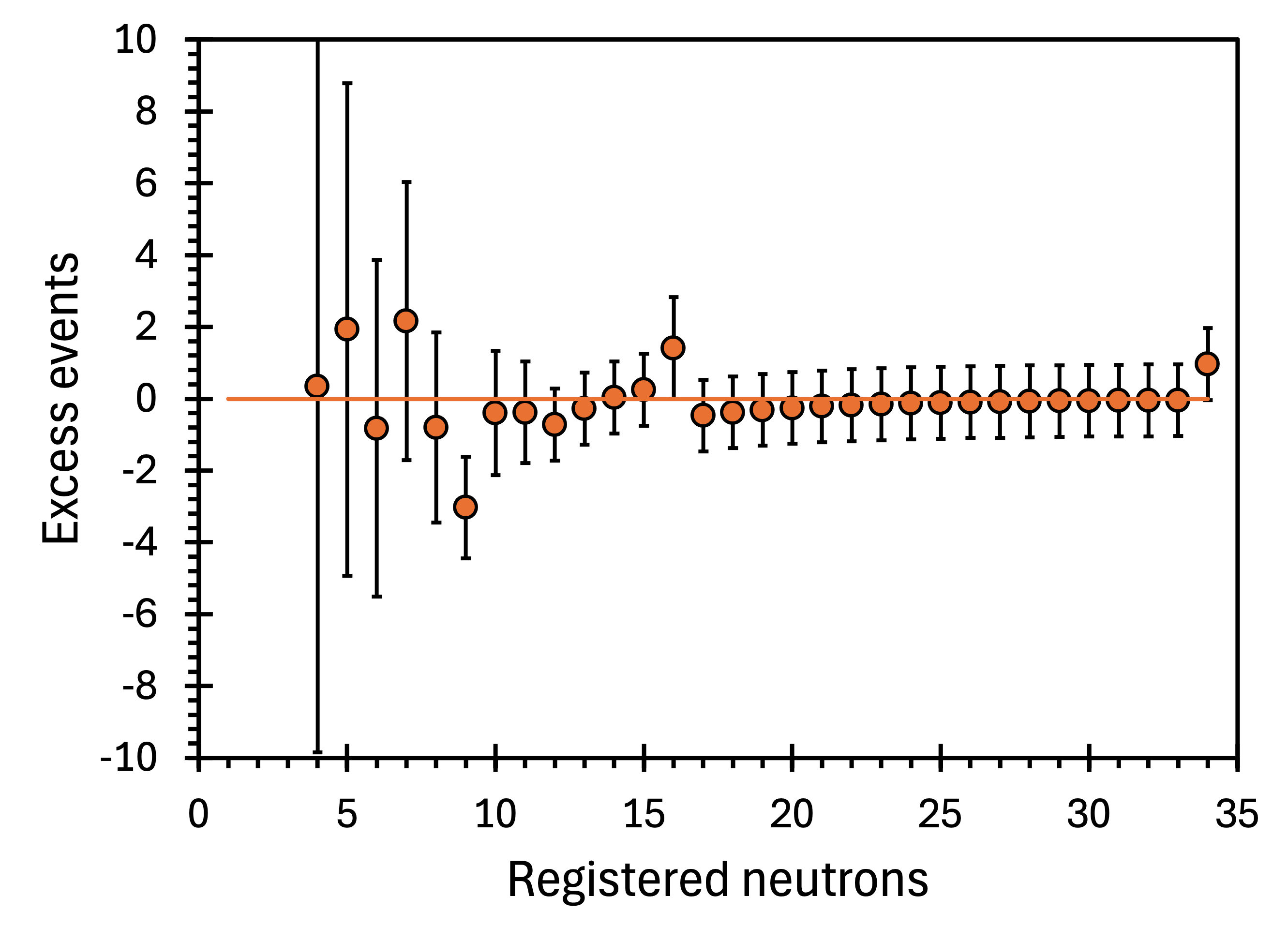
Unlike in the Pb case, no excess was detected with the Cu target. Such an outcome is not obvious, although differences in density, atomic and mass numbers between lead and copper are noticeable. Cu has 8.96 g/cm³ density, $Z=29$ , $A=63.546$ , while Pb has 11.34 g/cm³, $Z=82$ , and $A=207.2$ . In addition, while Pb is nearly transparent to thermal neutrons, this is not the case with Cu. Nevertheless, the lack of excess events in the Cu spectrum strengthens the credibility of our analysis by proving that if the power-law description of the neutron multiplicity spectra is adequate, we can replicate it.

7 JYFL Setup and Measurements

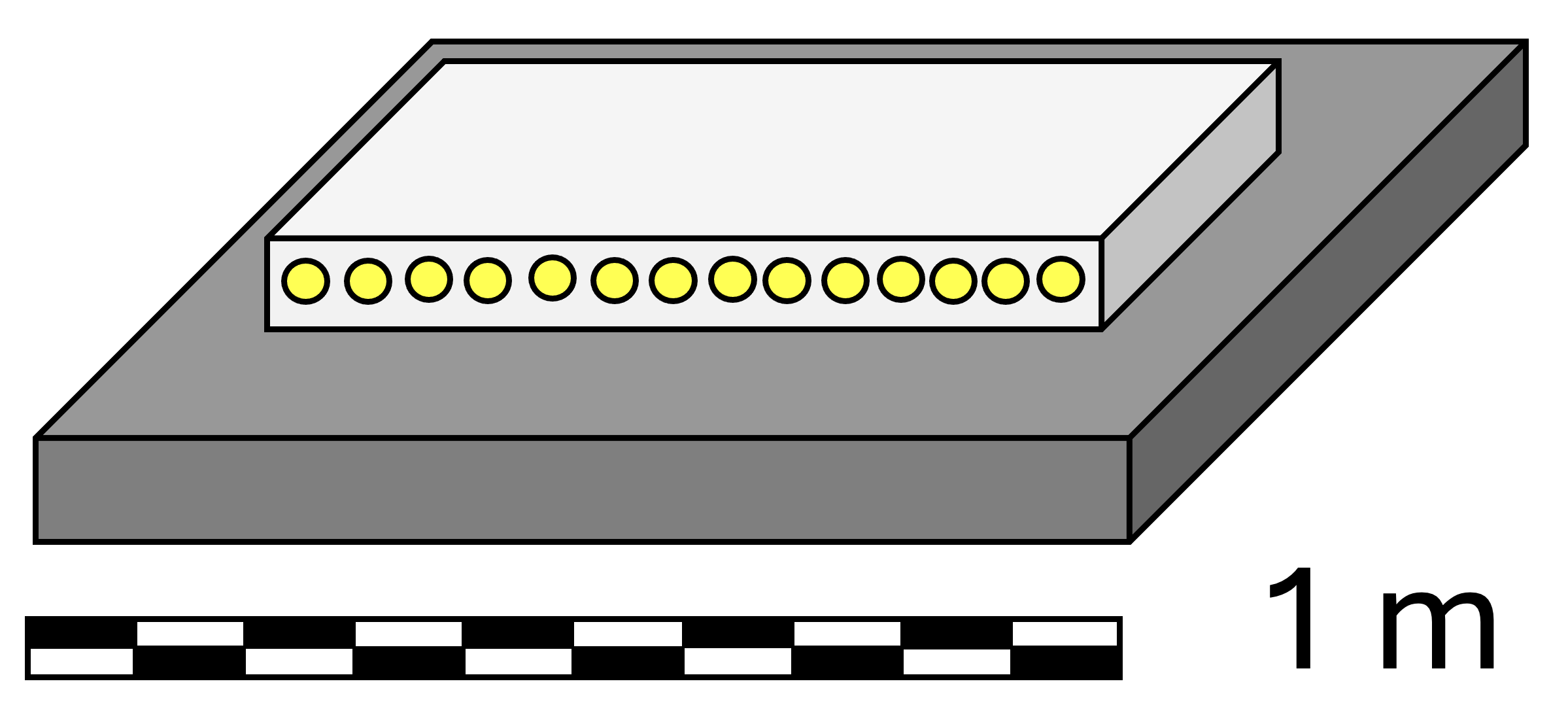
To reach the Five Sigma discovery level, we intended to conduct the measurements 1.4 km underground at $\sim$ 4000 m.w.e. The muon rate at that depth is only 9.5 muons per square meter per day [17]. Consequently, the muon-induced neutron multiplicity spectrum would be highly suppressed, enabling nearly background-free registration of anomalies. The planned setup was described in [30]. As the available funding to realise the proposed experiment was inadequate, we have implemented a significantly simplified version, reusing the 14 NCBJ counters with NDAQ and arranging them as shown in figure 25. As the simplified experiment was designed and pre-assembled at the Department of Physics, University of Jyväskylä, known by its Finnish acronym JYFL, we refer it to as JYFL-setup.

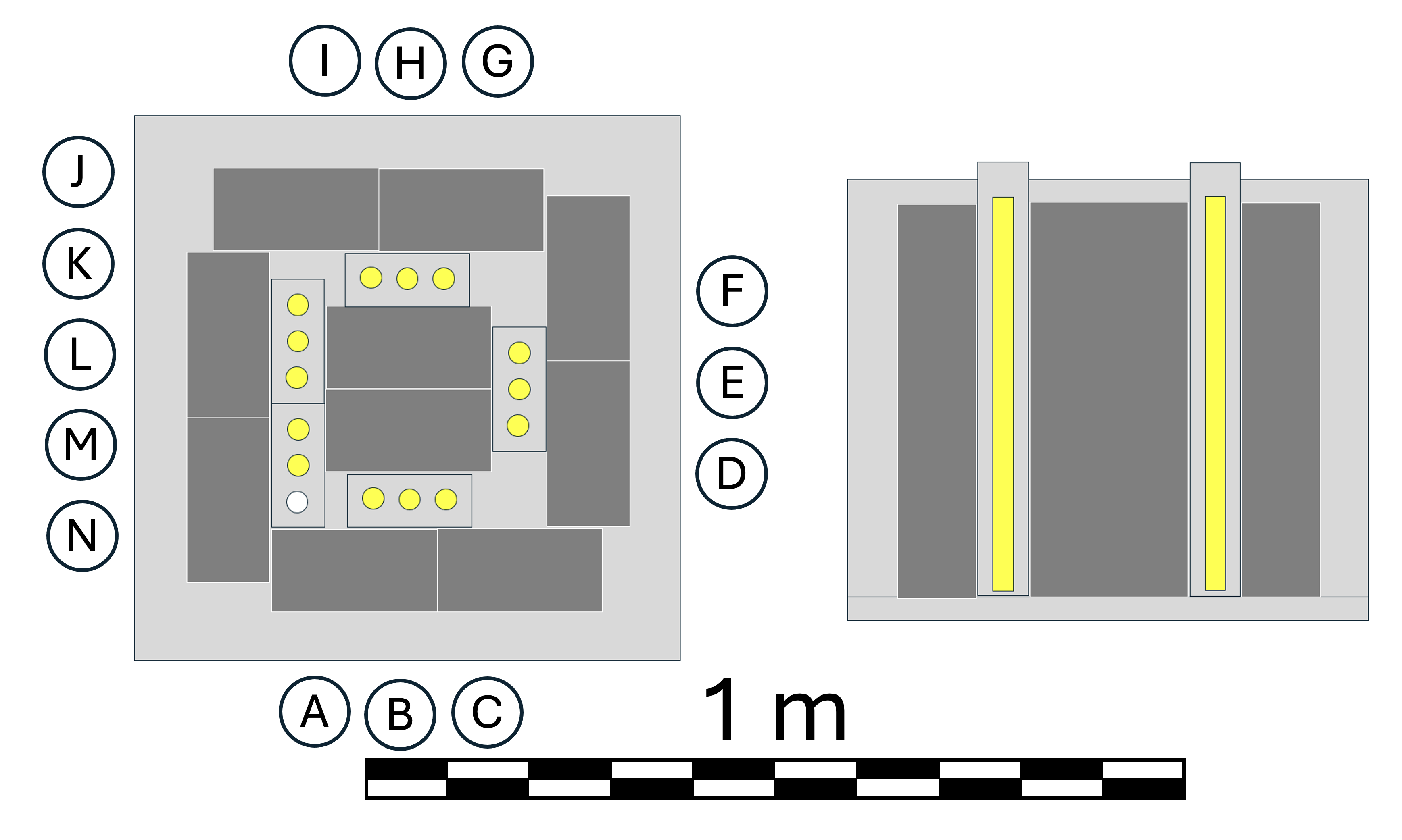
During the first 123 days of the experiment, high-multiplicity neutron events occurred at an average monthly rate of $1.5\pm 0.6$ . In total, six such events were recorded. The event spacing followed the exponential distribution predicted by the Poisson distribution. The detection date, time and time difference between the registered neutrons of each event are listed in table LABEL:tab:tab2, and the final neutron multiplicity spectrum is shown in figure 26. The event with multiplicity m=13 is consistent with emission from the central stacks, indicating the actual multiplicity of $M\sim 75\pm 20$ . The three $m=6$ and two $m=4$ events are consistent with emissions from the peripheral stacks, indicating $M\sim 76\pm 40$ . These results are consistent with the most prominent peak (at $M=74\pm 7$ ) observed at 583 m.w.e. and listed in table 1.

Table 2: Parameters of all high-multiplicity neutron events collected with the JYFL setup. The trigger time of each event is given with one-minute precision. The trigger starts the high-accuracy clock, so all the subsequent signals are timed with a one-microsecond step. The triggering pulse has the time after trigger equal to zero.

Multiplicity	Date	Trigger time	Comment
6	6.12.2022	21:04	BOT
Detector #	Placement	Time after trigger [ $\mu s$ ]
2018-02	B	0	neutron
2018-04	D	1	neutron
2019-03	M	1	neutron
2018-03	C	3	neutron
2018-01	A	56	neutron
2018-06	F	56	neutron
Multiplicity	Date	Trigger time	Comment
6	10.12.2022	3:18	BOT
Detector #	Placement	Time after trigger [ $\mu s$ ]
2018-05	E	0	neutron
2018-04	D	13	neutron
2018-03	C	20	neutron
2018-01	A	42	neutron
2018-01	A	92	neutron
2018-03	C	229	neutron
Multiplicity	Date	Trigger time	Comment
6	15.1.2023	14:16	LEFT
Detector #	Placement	Time after trigger [ $\mu s$ ]
2018-05	E	0	neutron
2018-01	A	8	neutron
2019-01	L	30	neutron
2018-09	I	138	neutron
2019-01	L	202	neutron
2018-01	A	469	neutron
Multiplicity	Date	Trigger time	Comment
4	21.1.2023	14:19	LEFT
Detector #	Placement	Time after trigger [ $\mu s$ ]
2018-10	J	0	not-neutron
2019-01	L	59	neutron
2018-09	I	70	neutron
2018-01	A	95	neutron
2019-09	K	117	neutron
2018-08	H	435	not-neutron
Multiplicity	Date	Trigger time	Comment
13	20.3.2023	8:46	CENT
Detector #	Placement	Time after trigger [ $\mu s$ ]
2018-06	F	0	overflow
2018-09	I	4	neutron
2019-01	L	4	neutron
2018-07	G	5	neutron
2018-08	H	6	neutron
2018-05	E	19	neutron
2018-02	B	30	neutron
2019-09	K	36	neutron
2018-08	H	42	neutron
2019-03	M	43	neutron
2018-06	F	55	neutron
2018-05	E	71	neutron
2018-09	I	106	neutron
2018-09	I	216	neutron
Multiplicity	Date	Trigger time	Comment
4	28.3.2023	17:11	ambiguous
Detector #	Placement	Time after trigger [ $\mu s$ ]
2018-09	I	0	neutron
2018-01	A	7	neutron
2018-01	A	34	neutron
2018-08	H	226	neutron

Strangely, no high-multiplicity events were recorded during the following 542 days of the run. If the rate of $1.5\pm 0.6$ events per month ( $1.3\pm 0.6$ per ton-month) determined during the first 123 days of the experiment is correct, the probability of not getting another such event in 18 months is negligible ( $<10^{-13}$ ). Since the detectors worked properly, the most likely cause for the lack of high-multiplicity events after the first 123 days of running is a malfunction of NDAQ. Evidently, the equipment must be inspected and checked, and the measurement must be repeated. Unfortunately, the 1.4 km deep level of the Pyhäsalmi mine is now closed for research projects, and we must rely on the available data. Assuming a malfunction soon after the 123rd day of running, we could only accept the results from the first four months of operation. However, it is also possible that the problems with the neutron detectors and the acquisition system started during the relocation from 210 m.w.e. and reinstallation at 4000 m.w.e. In this case, the data from the first four months of measurement were also unreliable. Only a new measurement may settle these questions.

8 Discussion

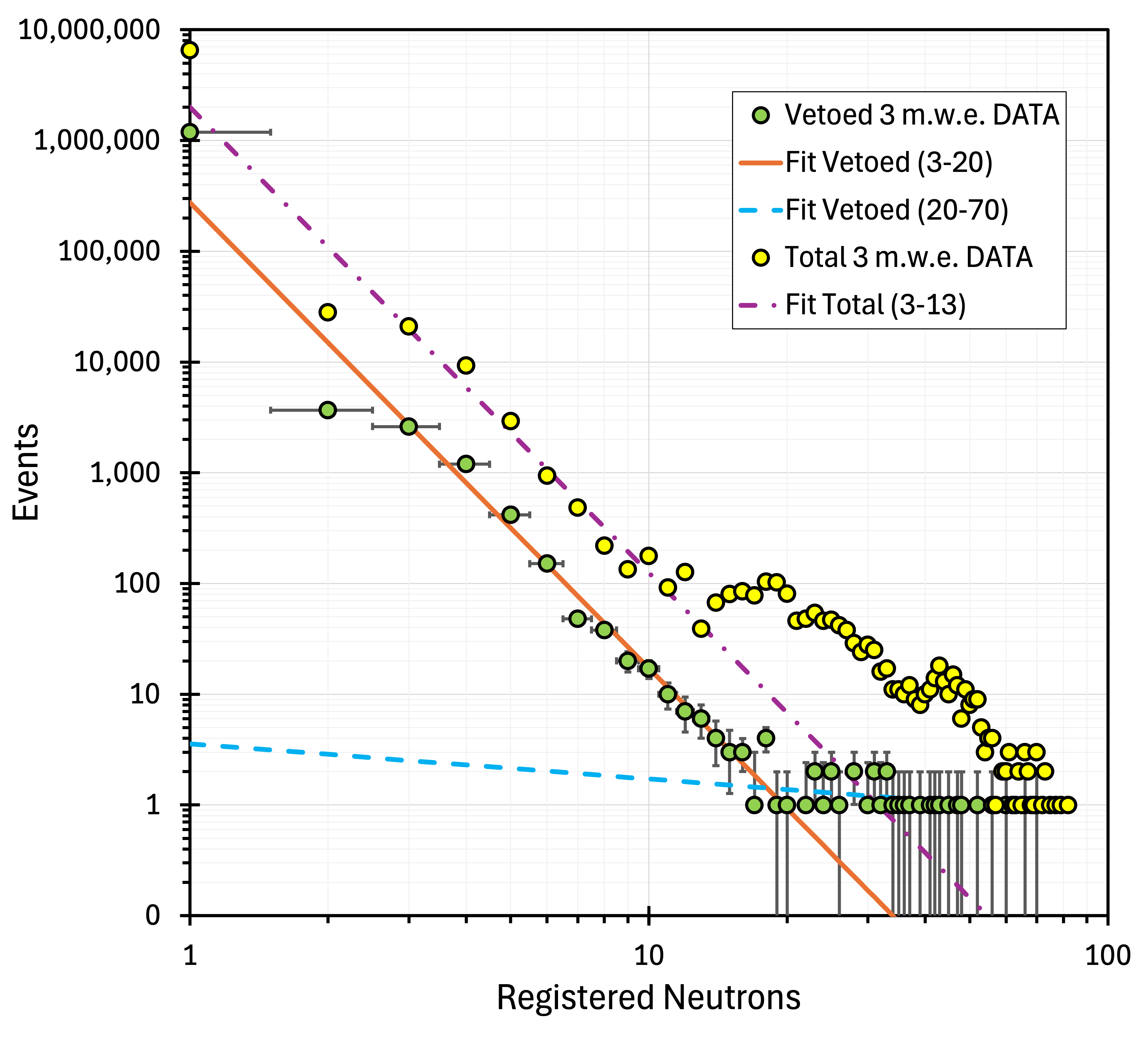
The main problems in the search for anomalies are low statistics and inadequate knowledge of the muon-induced neutron spectra. While the former may be solved with better experiments running longer and using larger targets, the latter is more challenging. While a generalised assumption that a power-law function describes muon-induced spectra is justified, the actual spectra show a more complex picture. The example from the shallow site is shown in figure 7, where the muon-suppressed (vetoed) NMDS data at 3 m.w.e. is displayed in the log-log scale and fitted with a power-law dependence in the neutron multiplicity range $3\leq m\leq 20$ (solid orange line, $p=4.21$ ) and $20\leq m\leq 70$ range (dashed blue line, $p=0.318$ ). There are two very different trends. What accounts for the dashed blue trend line if the red line represents muon-induced neutron production in Pb?

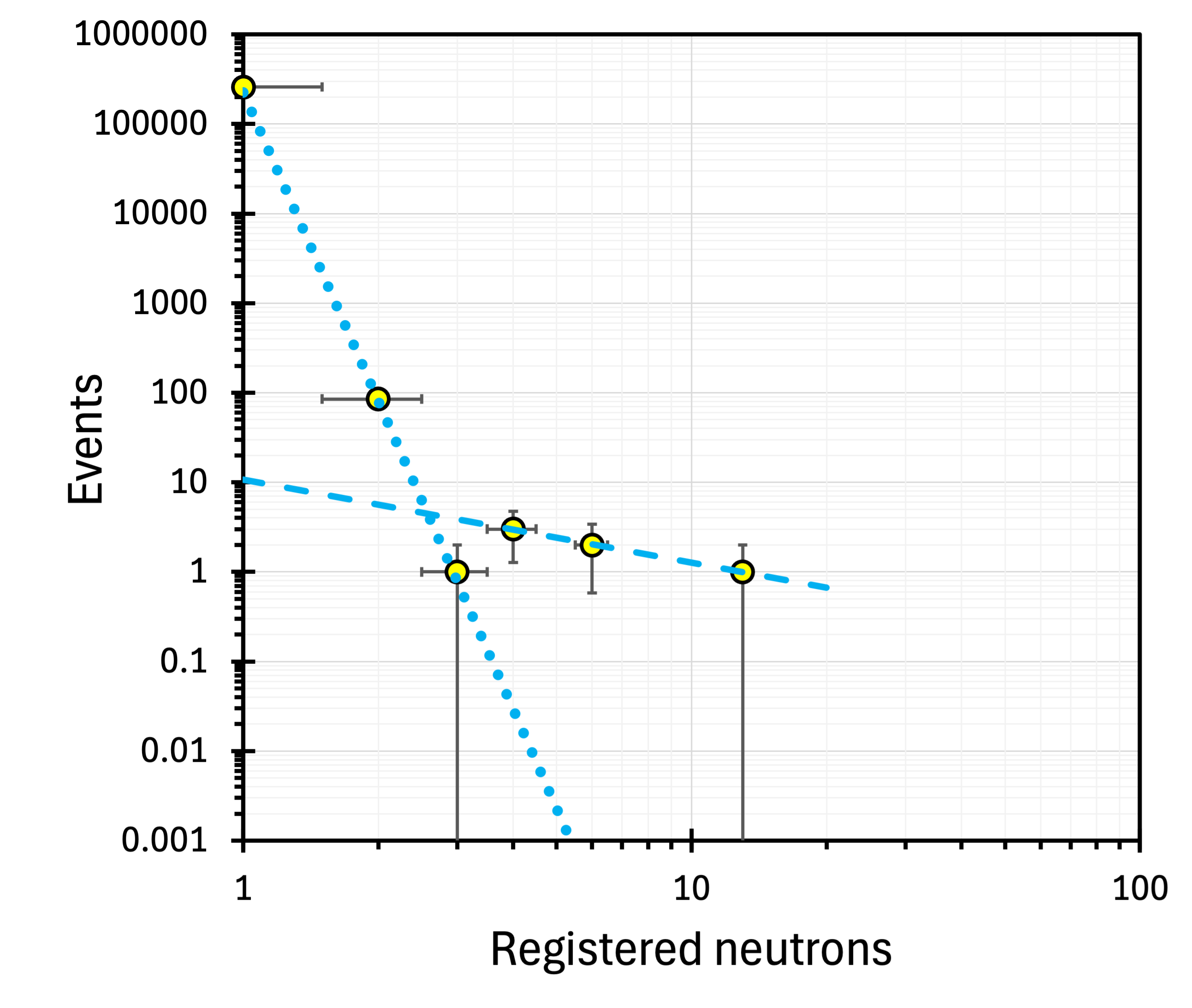
At greater depths, the crossover shifts to noticeably lower multiplicities. It is $m\approx 20$ at 3 m.w.e. (figure 7), and $m\approx 5$ at 1166 m.w.e. (figure 3). The dotted blue line in figure 3 is the power-law fit of the data at $2\leq m\leq 5$ ( $p=7.26$ ), and the dashed blue line at $5\leq m\leq 32$ ( $p=0.623$ ). The solid red line is the MC prediction reduced by a factor of two, as explained in section 4.3. The red dashed line is the Purdue fit. This one-component fit and the MC prediction overlap with only three points in the mid-section. The mismatch between the MC and 1166 m.w.e. data is also visible in figure 14, where linearised and normalised spectra are compared with the calculated MC trends. Unlike at 583 m.w.e., MC does not describe the 1166 m.w.e. neutron multiplicity spectrum. Finally, a similar two-component spectrum is very clear in the JYFL 4000 m.w.e. data (figure 26).

The NMDS 583 m.w.e. spectrum in figure 11 also reveals an interesting feature. While most of the data points follow the MC prediction (red line) and the $m=1$ point is evidently affected by the ambient neutron background, the points $2\leq m\leq 6$ follow their own trend (thin green dashed-dotted line, $p=4.21$ ) that is practically identical to that for total (thin dashed blue, $p=4.20$ ) and vetoed (thin purple dotted line, $p=4.20$ ) NMDS 3 m.w.e. trends.

Evidently, the simplified one power-law description of the neutron multiplicity spectra fails for the surface data collected with muon suppression (figure 7) and at depths below $\sim$ 1000 m.w.e. (figure 3 and figure 26). We treat the second component as an anomaly not reproduced by MC simulations. Therefore, analysing the data from 1166 and 4000 m.w.e., we assumed that the muon-induced contribution is described by the first (steeper) component and used it for background subtraction. With this assumption, unlike MC prediction (red line), the 1166 m.w.e. spectrum is well described by the four-peak hypothesis (the blue dotted line in figure 27). The integrated anomaly is $5.8\pm 3.2$ events, i.e., $10\pm 5$ events per ton-month.

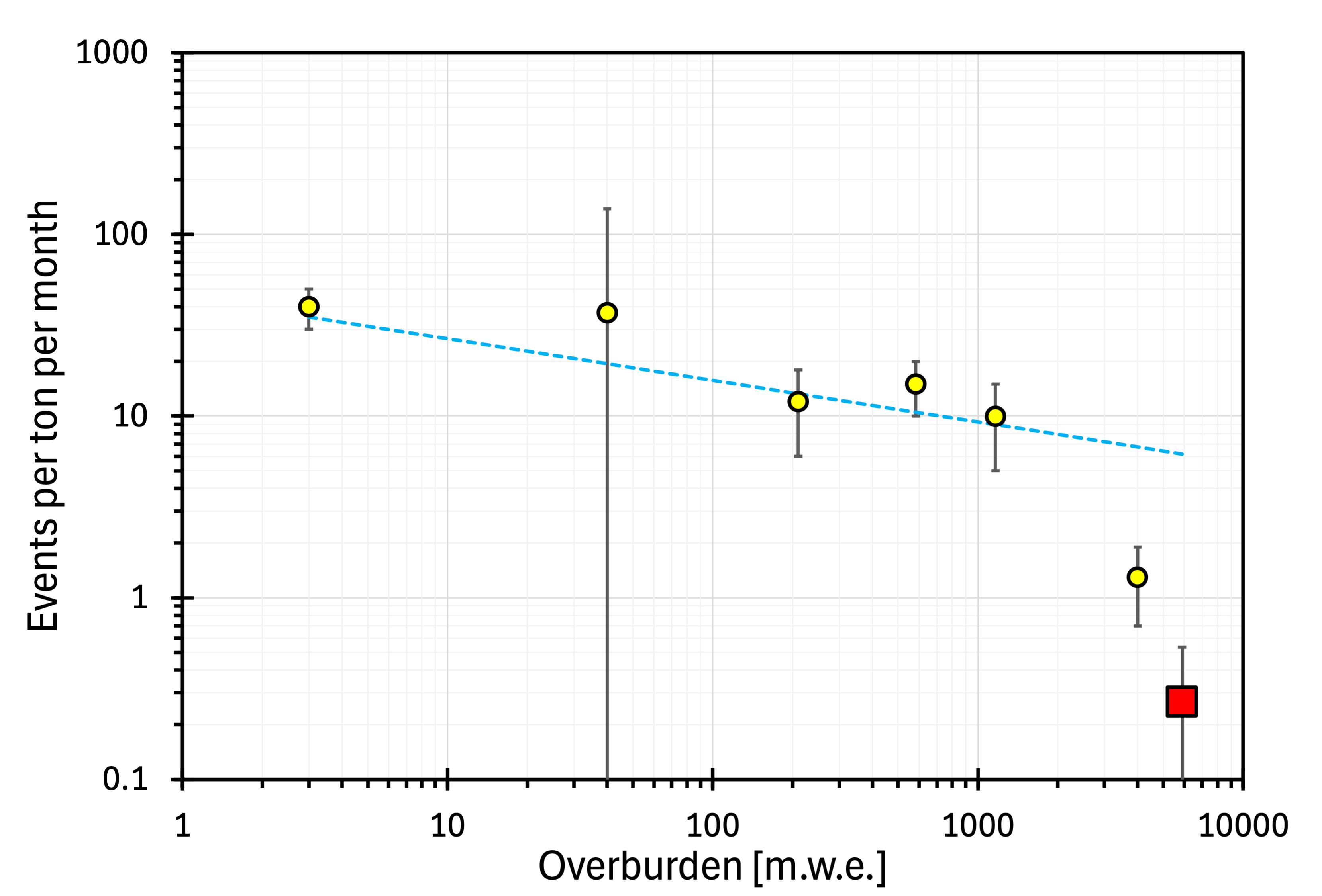
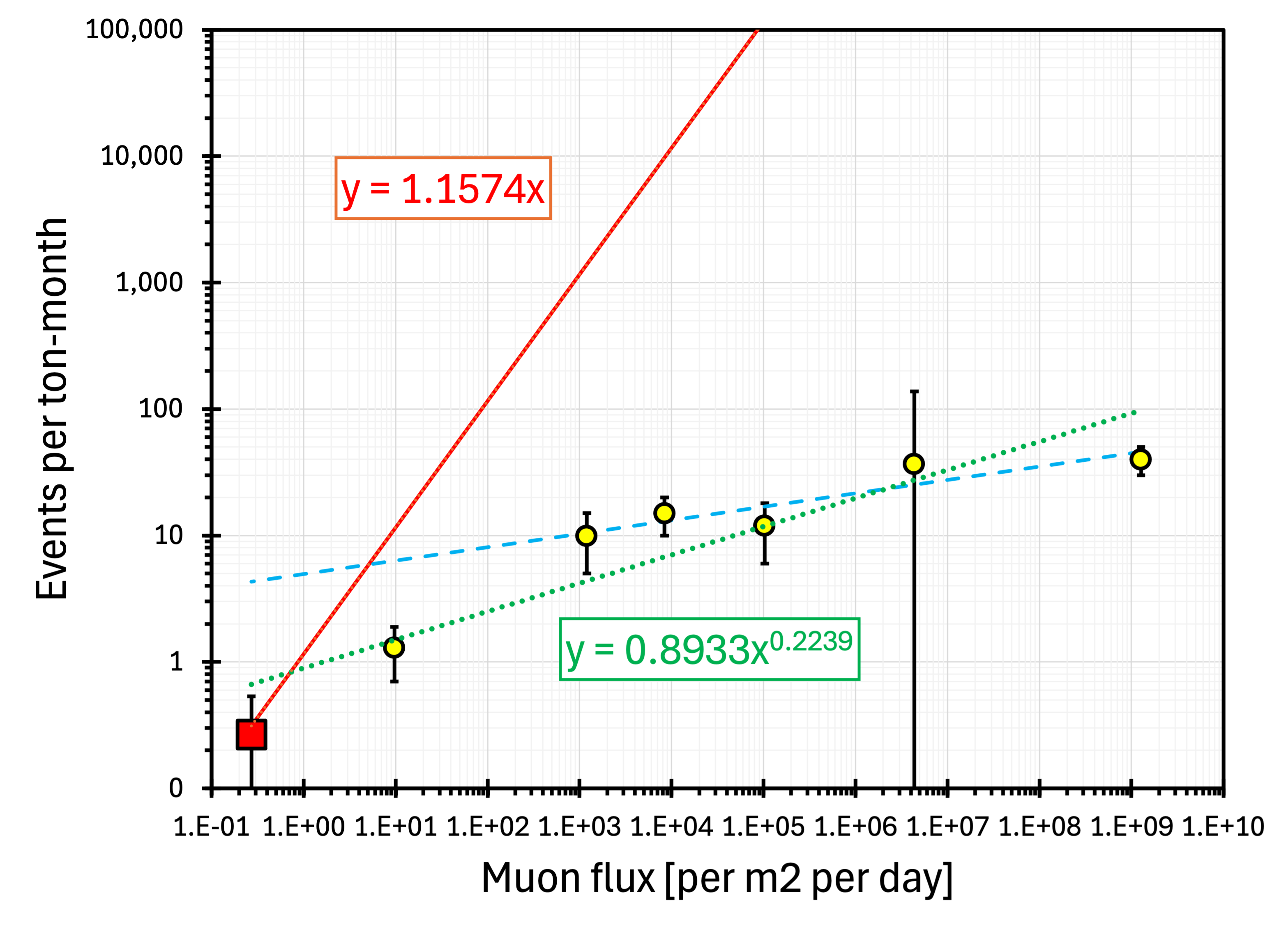
The four-month measurement with the JYFL setup at 4000 m.w.e. detected six high-multiplicity anomalies separated from the steep dependence marked as a blue dotted line in figure 26 and interpreted by us as a muon-induced portion of the spectrum. The outcome of the measurements is summarised in table 3 and shown as a function of overburden in figure 28. The data originate from measurements at five locations, ranging in depth from 3 to 4000 m.w.e. The yield of excess neutrons emitted from Pb gently decreases with depth. The dashed trend line in figure 28 is based on the five shallowest points. The trend predicts 6.7 excess events per ton per month at 4000 m.w.e., while the measured value is only $1.3\pm 0.6$ . As explained above, the lower-than-expected outcome may be related to NDAQ malfunctions arising from the hasty relocation of the setup from the 210 to the 4000 m.w.e. site. On the other hand, when the anomalies are plotted as a function of muon flux (figure 30), all data points align reasonably well.

Overburden	Muon flux	Anomaly	Stat. error
m.w.e	$\mu$ /m²/s	events/ton/month
3	$1.80\times 10^{2}$	40	10
40	$5.04\times 10^{1}$	37	101
210	$1.19\times 10^{0}$	12	6
583	$9.74\times 10^{-2}$	15	5
1166	$1.39\times 10^{-2}$	10	5
4000	$1.12\times 10^{-4}$	1.3	0.6

Table 3: Observed anomalies and calculated muon fluxes.

At this point, we cannot be certain about the reality of the anomalies, and we do not have a solid explanation for their existence. Nevertheless, high-multiplicity neutron sources other than cosmic-ray-induced muons remain a valid alternative as the event rate per ton at different depths differs from the muon flux by several orders of magnitude. For instance, the excess may be related to an indirect WIMP decay/annihilation via weak interaction with a Pb nucleus. If such an indirect process occurs, the setup consisting of a Pb target surrounded by neutron counters would be able to detect indirect Spin Independent WIMP-nucleon annihilation cross section at the level of $\sim 10^{-45}$ cm² for WIMP masses between 0.1 and 10 GeV/c² [16]. For indirect Spin-Dependent annihilation, the sensitivity limit would be $\sim 10^{-41}$ cm² [18]. Before further speculations, we propose confirming the existence and properties of the deduced anomalies in neutron multiplicity spectra with a dedicated experiment outlined in the Outlook section.

8.1 HALO experiment

One of the ongoing measurements that could contribute valuable data for studying anomalies in muon-induced neutron spectra is HALO – the Helium and Lead Observatory [31]. HALO has a 78,624 kg Pb target instrumented by 128 ultra-low-activity He-3 neutron counters, providing 368 m of active detector length. Located at SNOLAB with a 6000 m.w.e. overburden, HALO has been operating since May 2011 and is part of the SuperNova Early Warning System (SNEWS) [32].

Despite its potential, the analysis, simulation, and interpretation of HALO data are complicated by the detector’s irregular ’Swiss cheese’-like geometry, the strong position dependence of neutron detection efficiency, and the lack of position sensitivity in the He-3 counters. In contrast, the setup proposed in Section 9 – although smaller in scale – is more suitable for neutron multiplicity studies. It offers significantly improved instrumentation, position sensitivity and a much higher detector density, with 60 meters of active detector length per ton of target material, compared to only 4 m/ton in HALO.

To date, the only publicly accessible HALO neutron multiplicity spectrum was presented at the 2023 TAUP conference in Vienna [33]. The spectrum is marked as ‘preliminary’ and covers 5.6 years from a decade and a half of HALO operation. Figure 29 shows the HALO spectrum digitised manually from the poster, replotted in the log-log scale, and supplemented with statistical error bars.

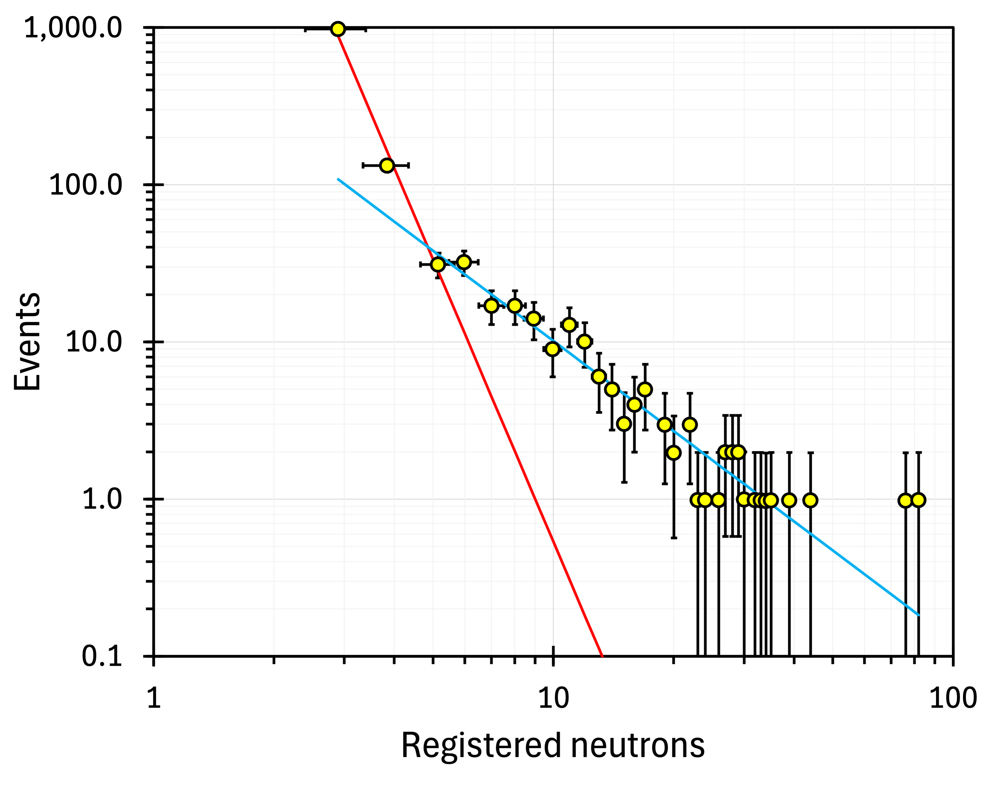
During the 5.6 years (2054 days) of exposure, only 4108 muons have reached HALO. And yet, the spectrum in figure 29 has 1302 events with multiplicities larger than two. We get over half a million events if we extrapolate the red line in figure 29 to the missing multiplicities ( $m=1$ and $2$ ), indicating a substantial background contribution.

Like at 1166 (figure 3) and 4000 m.w.e. (figure 26), there are two distinct components in the HALO neutron multiplicity spectrum. If we extrapolate and integrate the blue trend line in figure 29, we get 1412 events, that is 0.27 events per ton per month. Assuming that the blue component in figure 29 represents anomalies, we can add it (as a red square) to figure 28 and figure 30. As both the HALO spectrum and our analysis of their data are preliminary, we attribute arbitrary 100% error bars to that point (red square). It follows the trend of a mild muon flux dependence set by our results (the green dotted line in figure 30). For comparison, the thick red line in figure 30 illustrates the trend for events directly proportional to the muon flux.

9 Outlook

Although the persistence of the observed anomalies is compelling, their statistical significance falls short of the desired five sigma discovery level. To tackle this challenge, we have established the NEMESIS Collaboration, dedicated to NEutron MEasurementS In in Subterranean locations. Following the closure of the Pyhäsalmi mine, we are seeking new collaborators and funding to relocate the measurements to a new deep underground site. Further, in partnership with Proportional Technologies, Inc., we are developing a high-efficiency, low-background, low-cost neutron detector array using boron-coated straws (BCS). Each straw is a copper tube, 15 mm in diameter, lined on the inside with a thin layer of boron carbide (¹⁰B₄C) that is 96% enriched in the ¹⁰B isotope. The length of the BCS is adapted to the requirements. Thermal neutrons are converted into secondary charged particles via the B( $n,\alpha$ ) reaction: ¹⁰B + $n\rightarrow\ ^{7}$ Li $+\alpha$ . BCS-based detectors [34] are employed, e.g., to detect radioactive materials by the United States Department of Homeland Security [35] and by the LOKI broadband Small Angle Neutron Scattering (SANS) instrument at the European Spallation Source.

The current conceptual design of the proposed NEMESIS setup is illustrated in figure 31. It depicts the active elements (BCS) of two position-sensitive Large Area Neutron Detectors (LAND) positioned between three walls made of standard Pb bricks. The total Pb mass in this configuration will be 3402 kg. With hits in multiple straws, we can use the inverse square distance prediction to identify one of the three Pb walls where the emission occurred. Each LAND comprises 90 BCS. A digitiser-based data acquisition system records the time and position of the fired BSC for each detected neutron. As the two LANDs will be aligned perpendicularly to each other, the setup will ascertain the XY coordinates of high-multiplicity events, allowing us to determine the topology of each neutron burst. If emitted by a hypothetical WIMP decay/annihilation, all neutrons should originate from a point-like source in the Pb target. A spallation-like mechanism would generate neutrons along the muon trajectory, while multiple muon-induced hadronic reactions would indicate several point-like origins. The new experiment should distinguish between these scenarios. During the first year of operation, the setup in figure 31 would register an order of magnitude more high-multiplicity events than all our previous measurements combined. The setup can easily be expanded if needed by adding, at a moderate cost, alternating target/LAND layers.

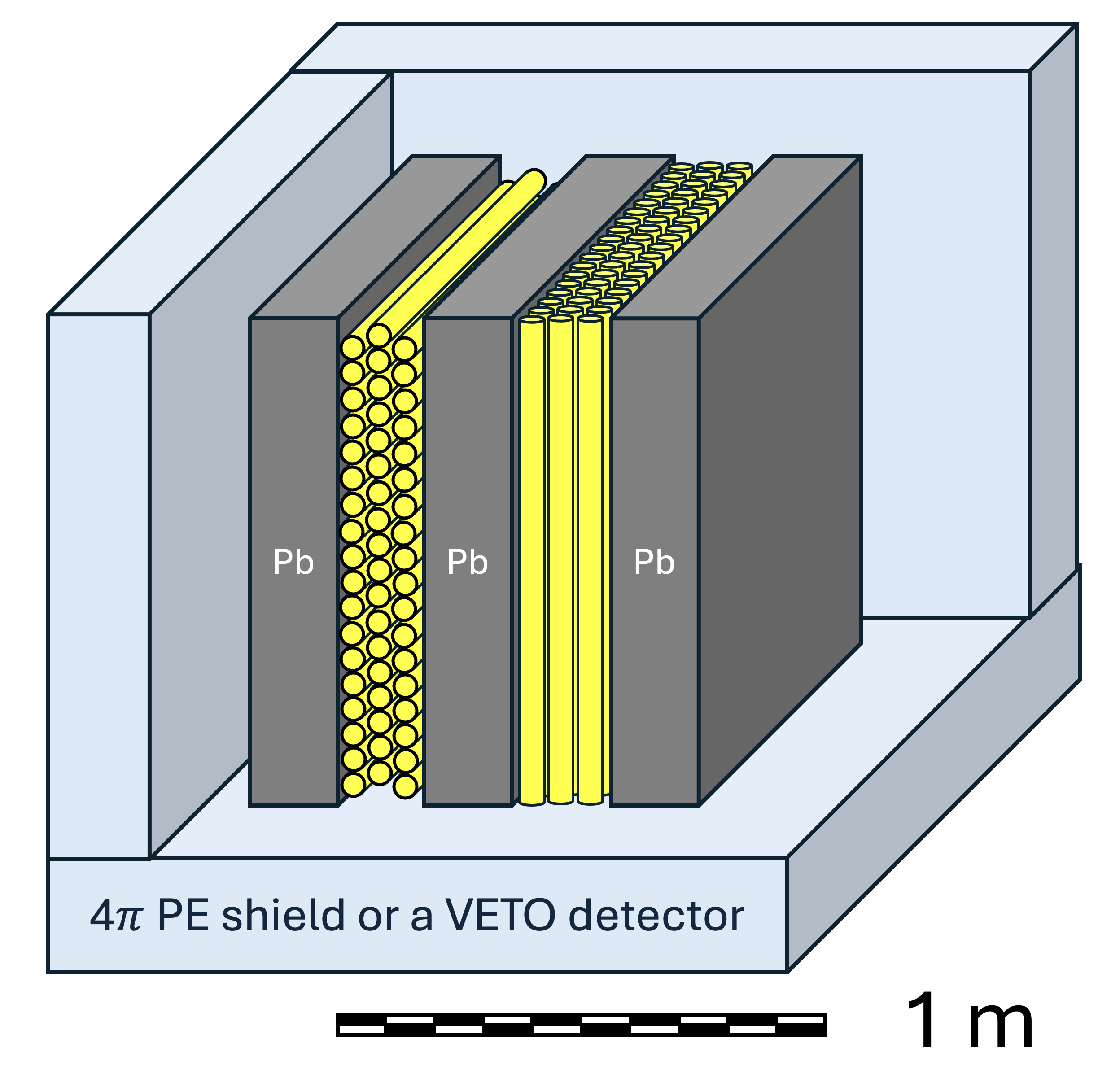
The final refinement of the setup will be a plastic scintillator-based charged particle tracking detector replacing the passive $4\pi$ PE shielding surrounding the target and LANDs. The $4\pi$ coverage is desired to distinguish between the traversing muons and particles emitted from the target. The former would trigger two sides of the veto cube, and the latter would only trigger one. Funding permitting, we look forward to realising this project soon.

10 Summary

•

We have analysed neutron multiplicity spectra measured with the NMDS setup (figure 1 and figure 6) at 3, 583 and 1166 m.w.e., the NCBJ setup (figure 19) at 40 and 210 m.w.e., and the JYFL setup (figure 25) at 4000 m.w.e.
•

The Purdue team’s detailed MC simulations are available for the NMDS setup at 583 and 1166 m.w.e. They conclude, in agreement with other published simulations using both Geant4 and Fluka, that a $k\times m^{-p}$ power-law function approximates the muon-induced neutron multiplicity spectra.
•

With the increase of overburden, the slope parameter $p$ remains roughly constant, while the amplitude parameter $k$ diminishes with the declining muon flux.
•

Our analysis indicates that the emergence of an anomalous component in neutron multiplicity spectra makes a single power-law approximation inadequate.
•

The anomalous structures can be detected in linearised and normalised integrated neutron multiplicity spectra (figure 10). Their shape differs from single power-law fits to the data and parametrised MC simulation results (figure 14).
•

At 1166 and 4000 m.w.e., the anomalous second component is already visible in unprocessed neutron multiplicity spectra (figures 3 and 26).
•

For a quantitative assessment of the anomalies, one must know or assume the background resulting from the muon-induced neutron events.
•

When MC simulation results were unavailable, we approximated the muon-induced contribution by a power-law fit to the measured data.
•

The integrated background-subtracted spectra are shown in figures 8, 12, 16, and 22.
•

No anomalous excess was detected when a Cu target was used (figure 24).
•

For Pb, the relative prominence of the excess events increases with depth (figures 10 and 21).
•

Measurements with a rudimentary muon veto added to the NMDS setup at 583 m.w.e. indicate that the anomalies are not directly caused by traversing muons (figure 16).
•

Nevertheless, the absolute value of the excess slightly drops with overburden (figure 28) and increases with muon flux (figure 30).
•

The smoothed neutron multiplicity spectra at 583 m.w.e. have a structure (figure 17) resembling four Gaussian peaks (figure 18). The statistics are insufficient for conclusive assessment, but the peaks are consistent with anomalous neutron emissions with multiplicity $M=74\pm 7$ , $M=106\pm 11$ , $M=143\pm 14$ , and $M=214\pm 21$ . The shapes of the excess events detected in other locations (figures 22, 23, and 27) are consistent with the peak hypothesis.
•

The acquired evidence for the anomalies (figures 28, 30 and table 3) falls short of the five-sigma discovery threshold but justifies follow-up experiments.
•

To cross the five-sigma discovery threshold, we need at least an order of magnitude higher statistics. The setup described in the Outlook section is designed to accomplish it during its first year of operation.

Acknowledgments

Many scientists initially involved in this project are no longer with us or have left the research field. In particular, we acknowledge the contributions of Alexander A. Rimsky-Korsakov, Nikolay A. Kudryashev, and their former team members to the commencement of this research. We express our gratitude to Callio Lab [https://calliolab.com] for providing access to the underground locations and infrastructure of the Pyhäsalmi mine. We gratefully acknowledge financial support from the Helsinki Institute of Physics, TechSource, and the Wihuri Foundation. Our special thanks go to the Kerttu Saalasti Institute team at the University of Oulu, including Dr. Ossi Kotavaara, Mr. Jari Joutsenvaara, and Ms. Julia Puputti, for their assistance and support during the setting up and conducting of the measurements.

References

[1] V. Pěč, V.A. Kudryavtsev, H.M. Araújo and T.J. Sumner, Muon-induced background in a next-generation dark matter experiment based on liquid xenon, Eur. Phys. J. C 84 (2024) 481 [2310.16586].
[2] I. Abt et al., The muon-induced neutron indirect detection EXperiment, MINIDEX, Astropart. Phys. 90 (2017) 1 [1610.01459].
[3] H. Cao and D. Koltick, Cosmic Ray Induced Neutron Production in a Lead Target, 2401.11280.
[4] J. Billard et al., Direct detection of dark matter—APPEC committee report*, Rept. Prog. Phys. 85 (2022) 056201 [2104.07634].
[5] (XENON Collaboration), XENON collaboration, XENONnT analysis: Signal reconstruction, calibration, and event selection, Phys. Rev. D 111 (2025) 062006 [2409.08778].
[6] T.J. Weiler, On the likely dominance of WIMP annihilation to fermion pair+W/Z (and implication for indirect detection), AIP Conf. Proc. 1534 (2013) 165 [1301.0021].
[7] T. E. Ward, Electroweak Mixing and the Generation of Massive Gauge Bosons, in Proceedings of Beyond the Desert 2002, Klapdor-Kleingrothaus, H. V., ed., p. 171, IOP Publishing, Bristol and Philadelphia, 2003 [hep-ph/0404064].
[8] National Nuclear Data Center, “ENDF/B-VII.1.” https://www.nndc.bnl.gov/endf/, 2011.
[9] H.M. Kluck, Measurement of the Cosmic-Induced Neutron Yield at the Modane Underground Laboratory, Ph.D. thesis, KIT, Karlsruhe, 2013. 10.1007/978-3-319-18527-9.
[10] O. Nairat, J.F. Beacom and S.W. Li, Neutron tagging can greatly reduce spallation backgrounds in Super-Kamiokande, Phys. Rev. D 111 (2025) 023014 [2409.10611].
[11] J. Albrecht et al., The Muon Puzzle in cosmic-ray induced air showers and its connection to the Large Hadron Collider, Astrophys. Space Sci. 367 (2022) 27 [2105.06148].
[12] D. Mei and A. Hime, Muon-induced background study for underground laboratories, Phys. Rev. D 73 (2006) 053004 [astro-ph/0512125].
[13] T.E. Ward et al., “Search for WIMP Dark-Matter Inelastic Interactions using a Lead Target.” APS April Meeting, https://meetings.aps.org/Meeting/APR19/Session/G17.1, 2019.
[14] W.H. Trzaska et al., New NEMESIS Results, PoS ICRC2021 (2021) 514.
[15] W.H. Trzaska et al., DM-like anomalies in neutron multiplicity spectra, J. Phys. Conf. Ser. 2156 (2021) 012029.
[16] W.H. Trzaska et al., New Evidence for DM-like Anomalies in neutron multiplicity spectra, PoS TAUP2023 (2024) 083 [2311.14385].
[17] T. Enqvist et al., Measurements of muon flux in the Pyhasalmi underground laboratory, Nucl. Instrum. Meth. A 554 (2005) 286 [hep-ex/0506032].
[18] H. Cao, “Indirect detection search for dark matter,.” Purdue University Graduate School, PhD thesis, https://hammer.purdue.edu/articles/thesis/Thesis_HC_04242023_pdf/22685170, 2023. 10.25394/PGS.22685170.v1.
[19] Z. Debicki, K. Jedrzejczak, J. Karczmarczyk, M. Kasztelan, R. Lewandowski, J. Orzechowski et al., Helium counters for low neutron flux measurements, Astrophys. Space Sci. Trans. 7 (2011) 511.
[20] “ZdAJ-HITEC.” https://hitecpoland.eu/.
[21] Z. Debicki, K. Jedrzejczak, J. Karczmarczyk, M. Kasztelan, R. Lewandowski, J. Orzechowski et al., Thermal neutrons at Gran Sasso, Nucl. Phys. B Proc. Suppl. 196 (2009) 429.
[22] Z. Dębicki, K. Jędrzejczak, J. Karczmarczyk, M. Kasztelan, R. Lewandowski, J. Orzechowski et al., Neutron flux measurements in the Gran Sasso national laboratory and in the Slanic Prahova Salt Mine, Nucl. Instrum. Meth. A 910 (2018) 133.
[23] K. Polaczek-Grelik et al., Natural background radiation at Lab 2 of Callio Lab, Pyhäsalmi mine in Finland, Nucl. Instrum. Meth. A 969 (2020) 164015.
[24] “BSUIN webpage.” http://bsuin.eu/.
[25] K. Jędrzejczak, M. Kasztelan, J. Orzechowski, J. Szabelski and Z. Nieckarz, Environmentally resilient data collecting system optimized for measuring low density neutron flux, Nucl. Instrum. Meth. A 1065 (2024) 169493.
[26] M. Kasztelan et al., High-multiplicity neutron events registered by NEMESIS experiment, PoS ICRC2021 (2021) 497.
[27] Z. Debicki, K. Jedrzejczak, J. Karczmarczyk, M. Kasztelan, R. Lewandowski, J. Orzechowski et al., Measurements and interpretation of registration of large number of neutrons generated in lead: The role of particle cascades, Astrophys. Space Sci. Trans. 7 (2011) 101.
[28] P. Kuusiniemi et al., Performance of tracking stations of the underground cosmic-ray detector array EMMA, Astropart. Phys. 102 (2018) 67.
[29] W.H. Trzaska, L. Bezrukov, T. Enqvist, J. Joutsenvaara, P. Kuusiniemi, K. Loo et al., Possibilities for Underground Physics in the Pyhasalmi mine, in 13th Conference on the Intersections of Particle and Nuclear Physics, 10, 2018 [1810.00909].
[30] W.H. Trzaska et al., NEMESIS setup for Indirect Detection of WIMPs, Nucl. Instrum. Meth. A 1040 (2022) 167223.
[31] C.A. Duba et al., HALO: The helium and lead observatory for supernova neutrinos, J. Phys. Conf. Ser. 136 (2008) 042077.
[32] SNEWS collaboration, SNEWS 2.0: a next-generation supernova early warning system for multi-messenger astronomy, New J. Phys. 23 (2021) 031201 [2011.00035].
[33] S. Sekula for the HALO Collaboration, “Measurements from halo.” XVIII International Conference on Topics in Astroparticle and Underground Physics (TAUP2023) Contribution, https://indi.to/wwdTx, 2023.
[34] M. Fang, J. Lacy, A. Athanasiades and A. Di Fulvio, Boron coated straw-based neutron multiplicity counter for neutron interrogation of TRISO fueled pebbles, Annals Nucl. Energy 187 (2023) 109794 [2303.00675].
[35] J.L. Lacy, A. Athanasiades, C.S. Martin, L. Sun and G.L. Vazquez-Flores, The evolution of neutron straw detector applications in homeland security, IEEE Transactions on Nuclear Science 60 (2013) 1140.