Anomalous Induced Density of Supercritical Coulomb Impurities in Graphene Under Strong Magnetic Fields
Abstract
The Coulomb impurity problem of graphene, in the absence of a magnetic field, displays discrete scale invariance. Applying a magnetic field introduces a new magnetic length scale and breaks discrete scale invariance. Moreover, a magnetic field is a singular perturbation as it turns complex energies into real energies. Nonetheless, the Coulomb potential must be regularized with a length at short distances for supercritical impurities. We investigate the structure of the induced density of a filled Landau impurity band in the supercritical regime. The coupling between Landau level states by the impurity potential is non-trivial and can lead to several anomalous effects. First, we find that the peak in the induced density can be located away from the center of the impurity, depending on the characteristics of the Landau impurity bands. Second, the impurity charge is screened, despite the Landau impurity band being filled. Third, anticrossing impurity states lead to additional impurity cyclotron resonances.
I Introduction
Recently, the supercritical Coulomb impurity problem has been revived [1, 2, 3, 4, 5, 6, 7, 8, 9] in two-dimensional graphene [10]. (The problem of Coulomb impurity in three-dimensional systems was intensively investigated many years ago. For a comprehensive review, see Ref. [11].) It has been experimentally demonstrated that single-atom vacancies in two-dimensional graphene can stably host local charge. Using various experimental techniques, the supercritical regime can be achieved [12, 13]. In the absence of a magnetic field, the induced density [2, 3, 4, 5, 7] has several interesting properties. However, how electron-electron interactions would affect these results is not well-known. The purpose of this paper is to investigate the induced density of the Coulomb impurity in the presence of magnetic fields. The advantage of applying a magnetic field is that, in some cases, it reduces the effect of electron-electron interactions due to an excitation gap between the Landau levels. We find that impurity states exhibit several unusual properties and give rise to an anomalous induced density, in addition to anticrossings that lead to new impurity cyclotron resonances. Before we present our main findings, we provide a brief introduction of the Coulomb impurity problem both in the absence and in the presence of a magnetic field.
The continuum model Hamiltonian of the two-dimensional Coulomb impurity model in the absence of a magnetic field takes the following form
| (1) |
where is the Fermi velocity, represents the Pauli spin matrices, is the impurity charge, is the effective dielectric constant, and is the Pauli matrix in the direction. Additionally, represents a finite mass gap. In the presence of a strong Coulomb potential, to avoid pathological oscillations of wavefunctions towards the impurity origin, the impurity charge is introduced with a size of . This breaks continuous scale symmetry into discrete scale symmetry (see Appendix A for an explanation of this effect). The coupling strength is defined as the ratio between two energy scales,
| (2) |
where and In the absence of a magnetic field and zero mass gap , subcritical and supercritical regimes separate at the critical coupling strength [2, 4, 1, 6].
Nishida [7] showed that, in the absence of a magnetic field, discrete scale invariance in the induced density in the supercritical regime has the following form
| (3) |
where is the total angular momentum and is a -dependent regularization parameter. In the subcritical region, , only the scale-independent first -function term is present [2, 4, 3], with the analytical form of given in Ref. [5]. The noteworthy feature is that the universal function displays log-periodic and discrete scale invariance [7], characterized by
| (4) |
where is an integer. The induced density exhibits a power-law tail, , as . The role of screening [5] in this induced density in the presence of electron-electron interactions has not been well investigated.
In the Coulomb impurity problem in magnetic fields, regardless of the value of the magnetic field, the critical dimensionless coupling remains constant, [14]. The problem was investigated both below [15, 16, 14] and above [14, 17, 18] critical coupling . The continuum model Hamiltonian of the Coulomb impurity problem in a magnetic field reads
| (5) |
The graphene sheet lies in the plane, and we use a symmetric gauge with vector potential . The first term gives rise to graphene Landau levels with magnetic length . The Landau level energy in the absence of impurity and the gap is , where the magnetic energy scale is . Discrete scale invariance is broken because of this magnetic length scale. The probability densities of the Landau level states in the absence of the impurity potential form rings with width . However, in the supercritical region, there is another length scale, , as the Coulomb potential must be regularized for supercritical impurity potentials [14]. There are now two relevant dimensionless parameters,
| (6) |
where is the characteristic energy scale of the Coulomb impurity. The coupling strength is the ratio between the Coulomb energy and the Landau level energy spacing. Notice that despite a magnetic field being considered here, this coupling strength is identical to the one in Eq. (2). When is large, many Landau levels are coupled by the Coulomb potential. Note that is independent of . The other parameter characterizes the regularization parameter of the Coulomb impurity.
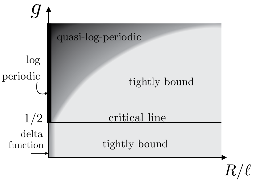
In the supercritical region , the following properties are found. (i) No complex energy solutions (resonances) are possible in the Coulomb impurity problem in magnetic fields: the effective potential does not allow resonant states since the vector potential diverges while the Coulomb potential goes to zero in the limit [19]. (ii) Regardless of the size of the mass gap , the critical dimensionless coupling strength remains a constant , unlike the case of zero magnetic field [6]. (iii) There can be different types of impurity bound states in a magnetic field: quasi-log-periodic [14] states for and tightly bound states for , as depicted in Fig. 1.
So far, we have briefly reviewed the basic properties of electronic wave functions of the Coulomb impurity problem. Now, we present our main results for the induced density in the supercritical regime, particularly focusing on strong magnetic fields. We consider only values of the dimensionless coupling strength where Landau impurity bands do not overlap. In such a case, the Landau level mixing in a filled impurity Landau band due to many-body effects is weak [20]. We investigate how the properties of induced density in the presence of a magnetic field compare to those in its absence. We find that the dimensionless induced density of such a filled Landau impurity band has the following structure in the supercritical region:
| (7) | ||||
with being the vector position from the impurity charge. The explicit form of will be presented below in Eq. (11). Here, the sum over is for all the states in the th filled Landau impurity band. We find the following similarities and differences in comparison to the zero-field mathematical structure of discrete scale invariance:
-
1.
We find, as in the presence of discrete scale invariance, that states with angular momentum strongly contribute to the anomalous induced density near . For the peak in the induced density is at and is most pronounced. However, for the peak in the induced density is away from the impurity center. The induced density displays small oscillations for , but without log-periodic oscillations for .
-
2.
There is no sharp change in the peak value of near the critical strength . The transition is smooth, but the peak value increases rapidly as exceeds .
-
3.
The second term of Eq. (7) leads to a unique effect present in a magnetic field: the induced density approaches a constant value for , where is the screening length. (In the absence of an impurity, the density of a filled Landau level is independent of and equal to this constant value.)
In addition, Landau impurity band states display anticrossings that lead to anomalous impurity cyclotro resonances.
Our paper is organized as follows. In Section II, we explain how our numerical method is implemented using a Hamiltonian matrix. Its eigenvalues and eigenstates that are relevant to the induced density are also explained. The properties of Landau impurity bands are explained in Section III. The induced density is computed in Section IV, and its properties are elucidated. Section V explains some unusual features of impurity cyclotron resonances due to the anticrossing of Landau impurity states. Finally, discussion and a summary are given in Section VI.
II Hamiltonian matrix and eigenstates
We find the eigenstates and eigenvalues of the problem numerically by converting it into the diagonalization of the Hamiltonian matrix.
We introduce the following wavefunctions to construct the basis states of the Hamiltonian:
| (8) |
where and are, respectively, the inter-Landau-level index and intra-Landau-level index. These two-component states are graphene Landau level states in the absence of an impurity, and their energy is given by [see below Eq.(5)]. The wave function of each component is defined in Appendix B. These wave functions are defined only for and , and are widely used in ordinary two-dimensional gases in a magnetic field [21]. In Eq. (8), when (equivalently, ), by definition. In this case, only the second component is non zero, and the wave function is chiral. The normalization condition of requires and for . Note that .
In constructing the basis states of the impurity problem in a symmetric gauge, it is useful to utilize the component of the total angular momentum:
| (9) |
as it is a good quantum number. Using , we find that the possible values of are half integers: . (The component of the total angular momentum operator is , where is the polar angle.) Table I lists possible values of for a given value of .
| Allowed values for a given | ||||||
| 0 | ||||||
By relabeling using index instead of , we now introduce the basis states of the Hamiltonian matrix:
| (10) |
The eigenstate wave function of the Hamiltonian with eigenenergy can be expressed as a linear combination of graphene Landau level states as follows:
| (11) |
where is defined as the Landau impurity band index. Formally, it is defined by taking the limit , where an impurity state reduces to a basis state: . In other words, only one term exists in Eq. (11), and . The expansion coefficients are column eigenvectors.
For a given value of , using these basis states , we form the total Hamiltonian matrix in the Hilbert subspace labeled by . The relevant Hamiltonian consists of a Dirac term, the Coulomb potential, and a mass term:
| (12) |
Since the graphene Landau level states are the basis, the matrix of the Dirac Hamiltonian in a magnetic field is a diagonal matrix with Landau level energies:
| (13) |
Here, the energy is measured in units of the magnetic energy . Note that employing the orthogonality in Eq. (30), the matrix elements of the mass term can be computed as
| (14) |
Matrix elements of the Coulomb potential are written as
| (15) |
which eventually can be simplified to the following form
| (16) | ||||
where , , , , , and . Here, is the normalization factor defined in Appendix B [see Eq. (31)].
To derive the above analytical form, we use the following identity of Laguerre polynomials [22]:
| (17) | ||||
where is the gamma function, the Pochhammer symbol is defined as , and is the generalized hypergeometric function.
In the supercritical region we must regularize the Coulomb impurity potential by introducing the radius of the impurity charge . For each value of , inter-Landau level numbers within are included (we will call the Landau level cutoff). The regularization parameter is related to the matrix dimension as follows:
| (18) |
This comes from the fact that the Landau level state with the highest index has this minimum length scale, namely, the distance between adjacent nodes in the wavefunction.
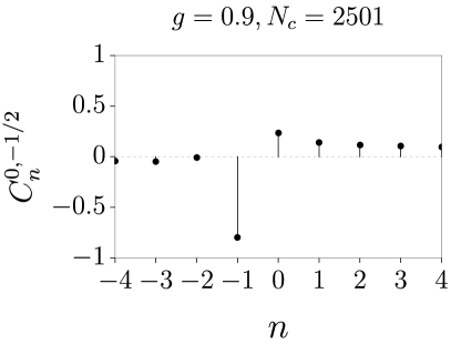
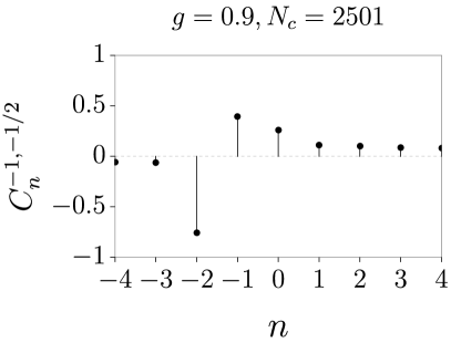
Some examples of the expansion coefficients are given in Fig. 2. Various plots of the probability densities of these eigenstates are shown in Appendix C.
III Landau impurity bands
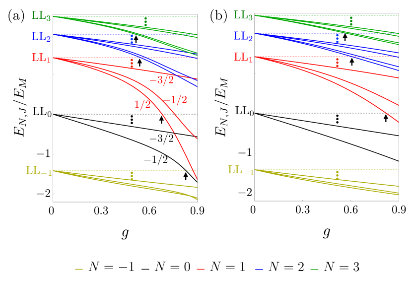
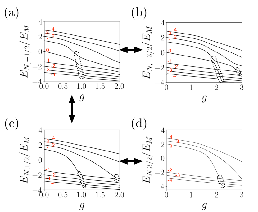
Plots of eigenvalues of Hamiltonian as a function of coupling strength are presented in Fig. 3. Figure 3(a) corresponds to a smaller value of compared to Fig. 3(b). The following points can be observed from the plot. Firstly, an impurity splits Landau level degeneracy. This splitting, measured in units of the magnetic energy , increases as coupling strength increases. The Landau levels and are mostly affected. The small magnetic field limit is approached with , i.e., [see Eq. (18)]. (Our numerical approach is not suited for investigating this limit because it requires a prohibitively large value of , meaning a prohibitively large Hamiltonian matrix.) Secondly, there are values of where Landau impurity bands do not overlap, and we will focus on these ranges of , specifically to the left of the black arrows. Finally, in this range of , the and Landau levels are strongly affected by the change in . In addition, the Landau level splitting is smaller for a smaller value of .
IV Induced density of a filled Landau impurity band
Suppose that states of a Landau impurity band are filled, and they do not overlap in energy with other Landau impurity band states. (There are values of for which Landau impurity bands do not overlap, positioned to the left of the black arrows in Fig. 3.) In such cases, mixing of Landau impurity band states with other band states due to many-body effects is weak, as demonstrated in Refs. [20, 23].
IV.1 Zero mass gap
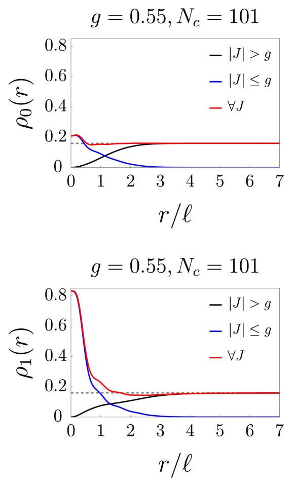
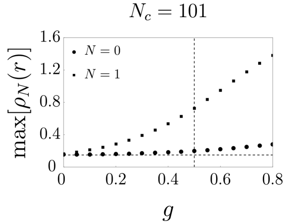
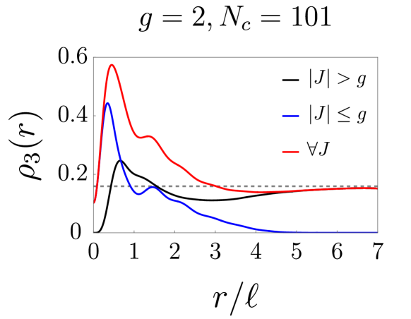
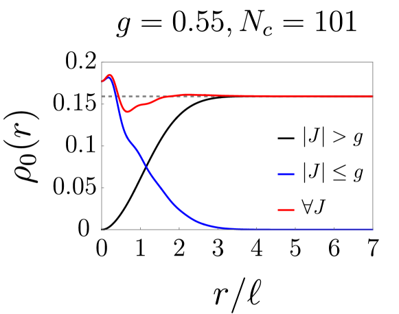
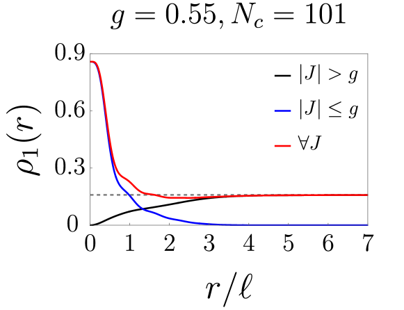
We first investigate the massless case with . The behavior of the induced density of a Landau impurity band can be rather different from that of zero magnetic field because discrete scale invariance is not present. We have computed the induced density in the supercritical regime for the values of and , as shown in Fig. 4. We find that no -function exists at , but a sharp narrowing of the induced density near the location of the impurity is present. This phenomenon is a precursor of the “fall to the center” of the electron bound to the impurity charge. Moreover, the position of the peak value of the induced density depends on the Landau impurity band index . For and the peak is near , as shown in Fig. 4. The red curves in Fig. 4 represent and , while the blue and black curves represent the first and second terms of the induced density given by Eq. (7). Note impurity band states with do not contribute to the induced density at . The peak value of is much larger than that of . This is because both Landau band impurity states with channels, and , contribute to it; however, for , only the state with , , does. For large the induced density of a filled Landau impurity band is . This corresponds precisely to the value of a filled graphene Landau level [23]. There is no sharp change in the induced density as a function of near . However, the peak value increases rapidly as exceeds . These properties of the induced density’s peak are illustrated in Fig. 5.
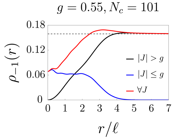
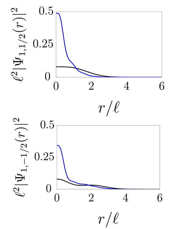
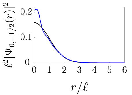
For some other values of , the peak is located away from . This effect becomes stronger for larger values of . An example with impurity band is illustrated in Fig. 6: The induced density is somewhat depleted near the center but accumulates near . We can explain this effect by qualitatively analyzing the contributions of angular momentum channels to the induced density. We observe that the peak in the induced density originates from . According to our numerical results, this impurity state may be approximated as
| (19) |
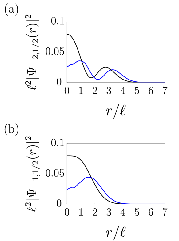
where are the basis states given in Eqs. (8) and (10). These basis states are visualized by black lines in Figs. 7(a) and 7(b): is peaked near , while is peaked at . [Equation (32) provides information about the location of the wavefunctions.] Hence, the combination of these two states causes the impurity state to peak at . The mixing between Landau levels induced by the impurity potential thus pushes these states and outward from the impurity center.
Another noteworthy feature is that for an impurity band with a larger and stronger coupling strength , the importance of the first term of Eq. (7) becomes clearer. The slope of the induced density near is accurately computed only when all the states with are included, as shown in Fig. 8 for and .
IV.2 Finite mass gap
The induced densities display the same qualitative behaviors when the gap value is finite: states with channels contribute to the peak, while other terms cause the corresponding induced density to approach a constant value of at large distances. Figure 9 displays induced densities for and for .
IV.3 Screening
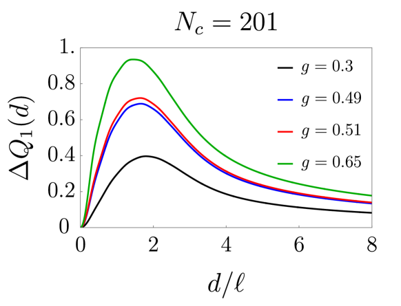
In this section, we study the screening of the impurity charge. It is convenient to examine the accumulated induced charge from the Landau impurity band within distance from the origin, defined as . Subtracting it from the total charge within the same distance in the absence of impurity, we obtain a charge difference that measures how much the impurity affects charge profiles within distance :
| (20) |
For a large distance , the influence of the impurity vanishes, . Hence, may be interpreted as the screening length. As coupling strength increases, screening length is expected to increase. A numerical result of the charge difference for the impurity band , plotted in Fig. 10, supports this expectation. Also, we observe that there is no sudden change in near the critical coupling strength , similar to the peak behavior in the induced density.
V Impurity cyclotron resonance
Impurity cyclotron resonance [24] may be used to detect the discrete energy levels in the energy spectrum. The optical matrix elements between the graphene Landau level states in the absence of impurity () are evaluated by using the formula [25]:
| (21) |
Here, we consider the current along the axis. (We recall that graphene is in the plane.) The explicit matrix elements for optical selection rules are given in Tables 2, which implies that is non zero only for . Combined with the implied rule of the Kronecker delta , we can infer that the allowed transitions must satisfy either or .
However, in the presence of a Coulomb potential, the optical matrix elements must be evaluated using Landau impurity band states. We find
where correspond to angular momentum increasing or decreasing by .
| 0 | 1 | 2 | 3 | ||||||
|---|---|---|---|---|---|---|---|---|---|
| 0 | 0 | 0 | |||||||
| 0 | 0 | - | 0 | 0 | |||||
| 0 | 0 | 0 | - | 0 | 0 | ||||
| 0 | 0 | 0 | 0 | ||||||
| 0 | 0 | 0 |
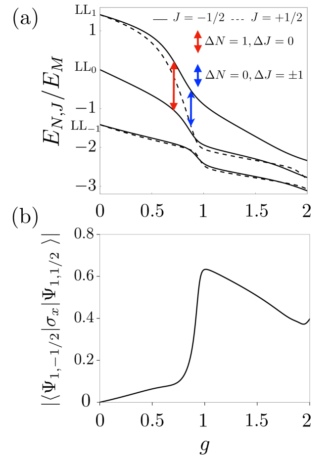
The form above suggests the possibility of anomalous transitions within the same impurity band, i.e., . In the limit the condition changes into , which is not optically allowed, as mentioned above. However, is possible at numerous finite values of because two impurity Landau levels may cross each other [17], as shown in Fig. 11. We compared our numerical results with the eigenspectrum obtained using the shooting method to solve the Dirac equation as described in Ref. [17], and obtained similar results using .
Let us analyze an example of an anomalous optical transition to gain a better understanding. Its matrix element is given by
| (23) |
This transition is depicted in Fig. 12(a), and the dependence of on is plotted in Fig. 12(b). We observe the following properties. (i) For small values of coupling strength , this optical matrix element is small. It can be explained by noting that with a small coupling strength, this optical matrix element is approximated by transition between graphene Landau level states, , which is forbidden because . (ii) For a strong coupling strength, such as with , the transition , which is allowed because , contributes significantly to . (iii) There is a crossover in as a function of , that occurs around , which is a consequence of strong Landau level mixing.
VI Discussion and Conclusions
We investigated the induced density of the supercritical Coulomb impurity in the regime where filled Landau impurity bands do not overlap and the effect of electron-electron interactions is significantly reduced. The strong coupling between graphene Landau level states by the impurity potential is non trivial and can lead to several anomalous effects. The induced density of a filled Landau impurity band can exhibit a sharp peak near the impurity center, much narrower than the magnetic length. However, due to strong coupling between graphene Landau levels, this peak can be located away from the center of the impurity, depending on the properties of different Landau impurity bands. We found, like in the presence of discrete scale invariance, that states with angular momentum strongly contribute to the induced density near . In addition, the impurity charge is screened despite the Landau impurity band being completely filled. We also showed that additional impurity cyclotron resonances exist that involve the anticrossing of Landau impurity band states.
While it is desirable to conduct a Hartree-Fock calculation [23], we do not anticipate qualitative changes in the induced density of a filled Landau impurity band, although some quantitative adjustments in the results are expected [26]. A scanning tunneling microscope [27] may be useful in investigating the anomalous induced density. Impurity cyclotron measurements [24] may also prove useful.
Appendix A Discrete scale invariance
The following simple example illustrates what discrete scale invariance is. Consider the function
| (24) |
with an imaginary scaling exponent . This function displays discrete scale invariance involving the exponent as follows:
| (25) |
We can rewrite the function as
| (26) |
This function exhibits log-periodic oscillations as a function of . In graphene discrete scale invariance also shows up [6] in the complex eigenenergies for ,
| (27) |
where is the half-integer angular momentum quantum number. One of the key factors of this mathematical structure is the appearance of the same exponent as in the log-periodicity of the wavefunctions given by Eq. (26), with the exponent:
| (28) |
For , the exponent is greater than zero, and the wavefunctions display log-periodic oscillations. The larger the coupling constant is, the more angular momentum channels are affected.
Appendix B Eigenstates of an Ordinary Two-Dimensional Electron gas in Magnetic Fields
In polar coordinates, the two-dimensional Landau level wave functions of an ordinary two-dimensional electron gas [21] are given for and by
| (29) |
where are generalized Laguerre polynomials. The component of the angular momentum of is . Note that, in contrast to graphene states, these states are one-component wave functions. Also, the definition of the component of angular momentum is different. Using the orthogonality of Laguerre polynomials
| (30) |
the normalization factor is derived as
| (31) |
with and . All the states decay exponentially as . One can show the following identity for the expectation value of :
| (32) |
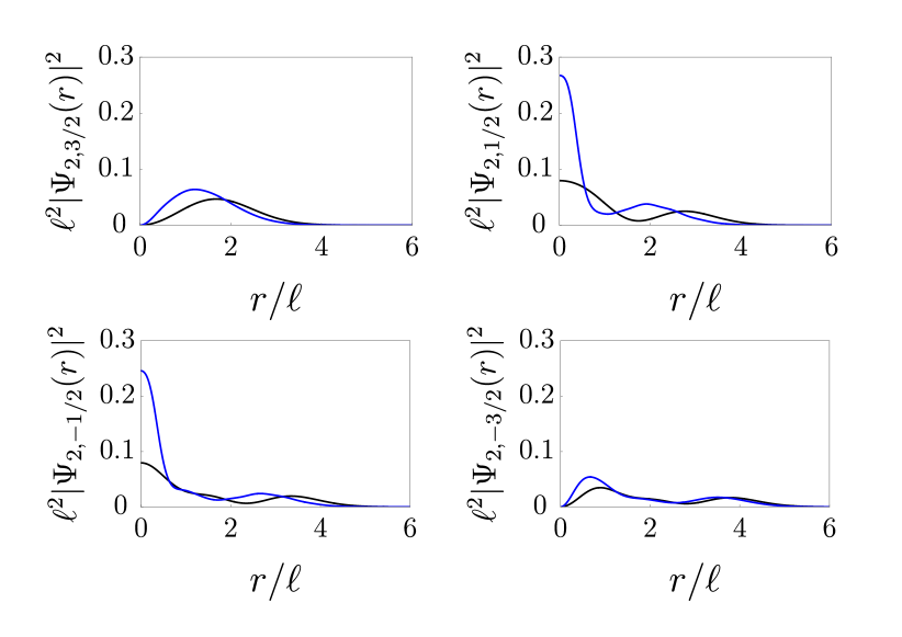
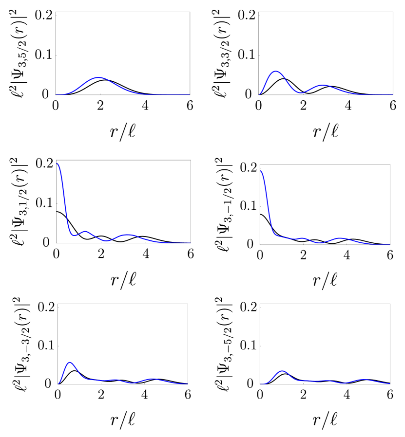
Appendix C Eigenstates
We analyze the properties of different impurity band states. The following points are worth noting:
- 1.
- 2.
References
- Khalilov and Ho [1998] V. Khalilov and C.-L. Ho, Dirac electron in a coulomb field in (2+1) dimensions, Modern Physics Letters A 13, 615 (1998).
- Pereira et al. [2007] V. M. Pereira, J. Nilsson, and A. H. Castro Neto, Coulomb impurity problem in graphene, Phys. Rev. Lett. 99, 166802 (2007).
- Biswas et al. [2007] R. R. Biswas, S. Sachdev, and D. T. Son, Coulomb impurity in graphene, Phys. Rev. B 76, 205122 (2007).
- Shytov et al. [2007] A. V. Shytov, M. I. Katsnelson, and L. S. Levitov, Vacuum polarization and screening of supercritical impurities in graphene, Phys. Rev. Lett. 99, 236801 (2007).
- Terekhov et al. [2008] I. S. Terekhov, A. I. Milstein, V. N. Kotov, and O. P. Sushkov, Screening of coulomb impurities in graphene, Phys. Rev. Lett. 100, 076803 (2008).
- Gamayun et al. [2009] O. V. Gamayun, E. V. Gorbar, and V. P. Gusynin, Supercritical coulomb center and excitonic instability in graphene, Phys. Rev. B 80, 165429 (2009).
- Nishida [2014] Y. Nishida, Vacuum polarization of graphene with a supercritical coulomb impurity: Low-energy universality and discrete scale invariance, Phys. Rev. B 90, 165414 (2014).
- Gorbar et al. [2018] E. V. Gorbar, V. P. Gusynin, and O. O. Sobol, Electron states in the field of charged impurities in two-dimensional Dirac systems (Review Article), Low Temperature Physics 44, 371 (2018).
- Zhu et al. [2009] W. Zhu, Z. Wang, Q. Shi, K. Y. Szeto, J. Chen, and J. G. Hou, Electronic structure in gapped graphene with a coulomb potential, Phys. Rev. B 79, 155430 (2009).
- Castro Neto et al. [2009] A. H. Castro Neto, F. Guinea, N. M. R. Peres, K. S. Novoselov, and A. K. Geim, The electronic properties of graphene, Rev. Mod. Phys. 81, 109 (2009).
- Reinhardt and Greiner [1977] J. Reinhardt and W. Greiner, Quantum electrodynamics of strong fields, Reports on Progress in Physics 40, 219 (1977).
- Mao et al. [2016] J. Mao, Y. Jiang, D. Moldovan, G. Li, K. Watanabe, T. Taniguchi, M. R. Masir, F. M. Peeters, and E. Y. Andrei, Realization of a tunable artificial atom at a supercritically charged vacancy in graphene, Nature Physics 12, 545 (2016).
- Wang et al. [2013] Y. Wang, D. Wong, A. V. Shytov, V. W. Brar, S. Choi, Q. Wu, H.-Z. Tsai, W. Regan, A. Zettl, R. K. Kawakami, S. G. Louie, L. S. Levitov, and M. F. Crommie, Observing atomic collapse resonances in artificial nuclei on graphene, Science 340, 734 (2013).
- Kim and Eric Yang [2014] S. Kim and S.-R. Eric Yang, Coulomb impurity problem of graphene in magnetic fields, Annals of Physics 347, 21 (2014).
- Ho and Khalilov [2000] C.-L. Ho and V. R. Khalilov, Planar dirac electron in coulomb and magnetic fields, Phys. Rev. A 61, 032104 (2000).
- Zhang et al. [2012] Y. Zhang, Y. Barlas, and K. Yang, Coulomb impurity under magnetic field in graphene: A semiclassical approach, Phys. Rev. B 85, 165423 (2012).
- Sobol et al. [2016] O. O. Sobol, P. K. Pyatkovskiy, E. V. Gorbar, and V. P. Gusynin, Screening of a charged impurity in graphene in a magnetic field, Phys. Rev. B 94, 115409 (2016).
- Moldovan et al. [2017] D. Moldovan, M. R. Masir, and F. M. Peeters, Magnetic field dependence of the atomic collapse state in graphene, 2D Materials 5, 015017 (2017).
- Kim et al. [2012] S. C. Kim, J. W. Lee, and S.-R. Eric Yang, Resonant, non-resonant and anomalous states of dirac electrons in a parabolic well in the presence of magnetic fields, Journal of Physics: Condensed Matter 24, 495302 (2012).
- Iyengar et al. [2007] A. Iyengar, J. Wang, H. A. Fertig, and L. Brey, Excitations from filled landau levels in graphene, Phys. Rev. B 75, 125430 (2007).
- Yoshioka [2002] D. Yoshioka, The Quantum Hall Effect, Springer Series in Solid-State Sciences (Springer Berlin, Heidelberg, 2002).
- Mavromatis [1990] H. A. Mavromatis, An interesting new result involving associated laguerre polynomials, International Journal of Computer Mathematics 36, 257 (1990).
- MacDonald et al. [1993] A. H. MacDonald, S.-R. Eric Yang, and M. Johnson, Quantum dots in strong magnetic fields: Stability criteria for the maximum density droplet, Australian journal of physics 46, 345 (1993).
- Goldman et al. [1986] V. J. Goldman, H. D. Drew, M. Shayegan, and D. A. Nelson, Observation of impurity cyclotron resonance in , Phys. Rev. Lett. 56, 968 (1986).
- Beenakker [2008] C. W. J. Beenakker, Colloquium: Andreev reflection and klein tunneling in graphene, Rev. Mod. Phys. 80, 1337 (2008).
- Kim et al. [2014] S. C. Kim, S.-R. Eric Yang, and A. H. MacDonald, Impurity cyclotron resonance of anomalous dirac electrons in graphene, Journal of Physics: Condensed Matter 26, 325302 (2014).
- Andrei et al. [2012] E. Y. Andrei, G. Li, and X. Du, Electronic properties of graphene: a perspective from scanning tunneling microscopy and magnetotransport, Reports on Progress in Physics 75, 056501 (2012).