Anomaly Detection with Test Time Augmentation and Consistency Evaluation
Abstract
Deep neural networks are known to be vulnerable to unseen data: they may wrongly assign high confidence scores to out-distribution samples. Recent works try to solve the problem using representation learning methods and specific metrics. In this paper, we propose a simple, yet effective post-hoc anomaly detection algorithm named Test Time Augmentation Anomaly Detection (TTA-AD), inspired by a novel observation. Specifically, we observe that in-distribution data enjoy more consistent predictions for its original and augmented versions on a trained network than out-distribution data, which separates in-distribution and out-distribution samples. Experiments on various high-resolution image benchmark datasets demonstrate that TTA-AD achieves comparable or better detection performance under dataset-vs-dataset anomaly detection settings with a running time reduction of existing classifier-based algorithms. We provide empirical verification that the key to TTA-AD lies in the remaining classes between augmented features, which has long been partially ignored by previous works. Additionally, we use RUNS as a surrogate to analyze our algorithm theoretically.
1 Introduction
Recently, deep neural networks have shown substantial flexibility and valuable practicality in various tasks [19, 23]. However, when deploying deep learning in reality, one of the most concerning issues is that deep models are known to be overconfident when exposed to unseen data [3, 13]. That is, although the deep models generalize well on unseen datasets drawn from the same distribution (i.e., test data), it incorrectly assigns high confidence to unseen data drawn from another distribution (i.e., out-distribution data). To solve the problem, anomaly detection [2] aims to separate unseen data from training data.
When testing deep neural networks, test time augmentation (TTA) utilizes the property that a well-trained classifier should have a low variance in predictions across augmentations on most data [38, 37]. However, this phenomenon is only explored and verified on data drawn from the training distribution (in-distribution). It is still unclear whether this property generalizes to other different distributions (out-distribution).
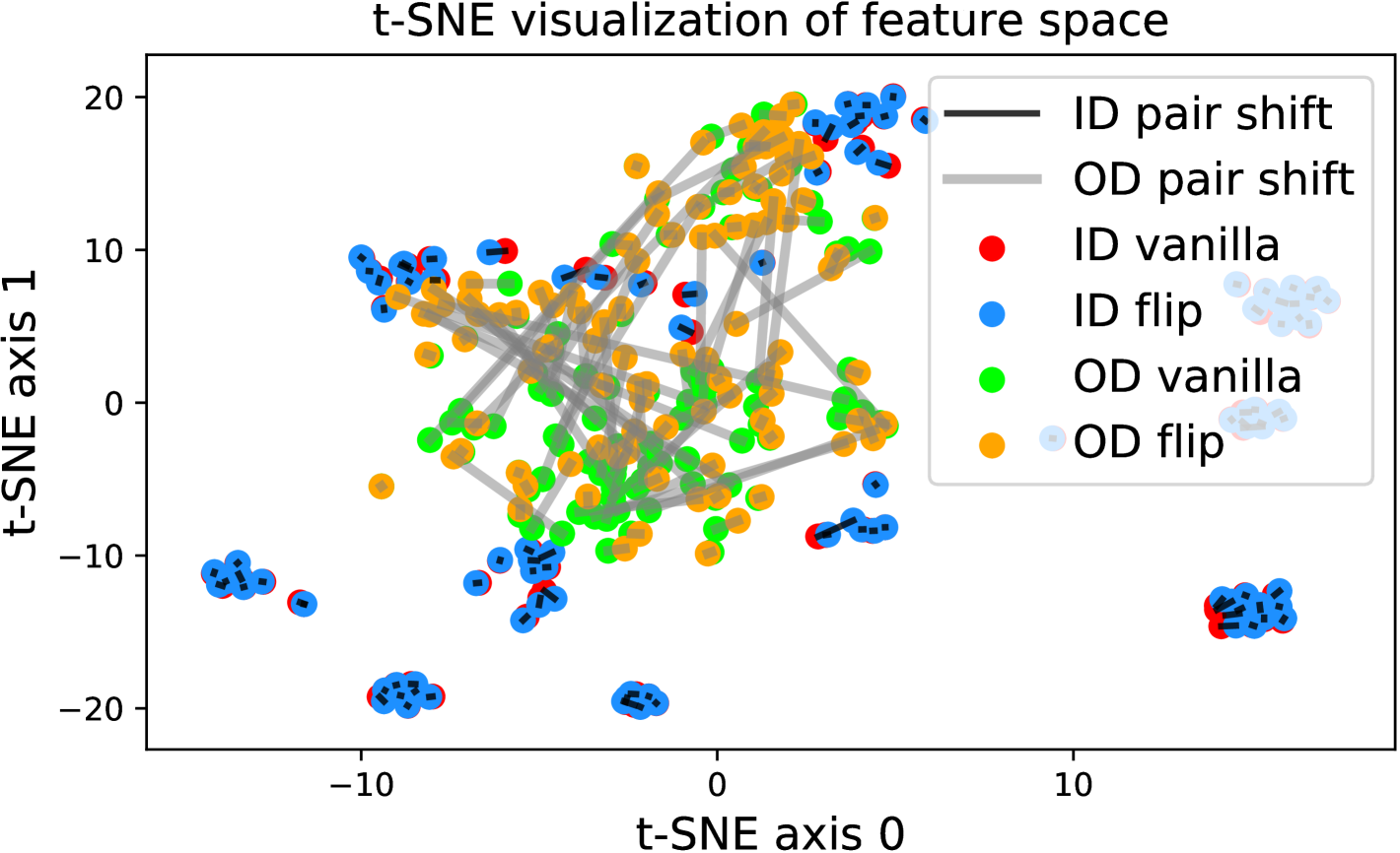
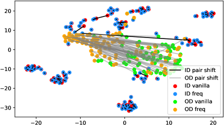
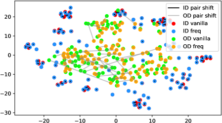
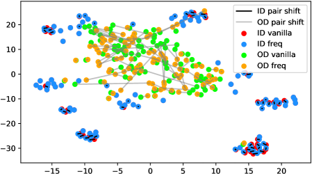
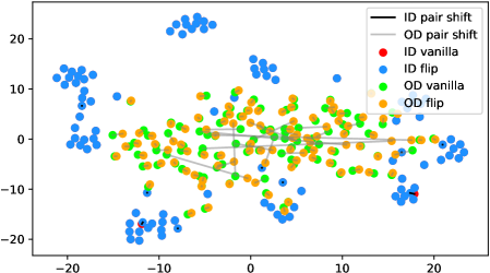
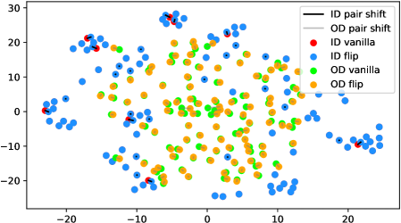
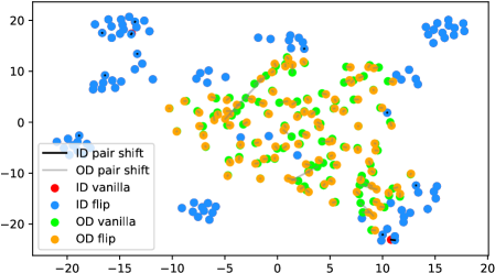
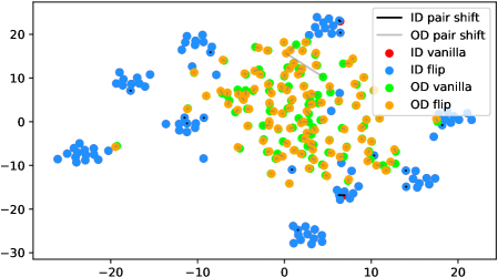
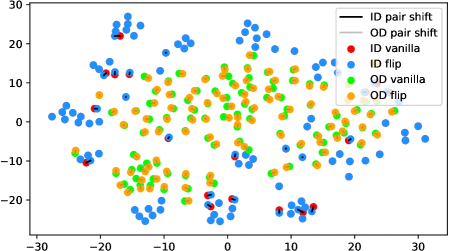
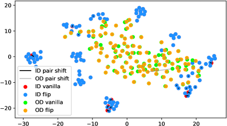
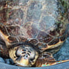
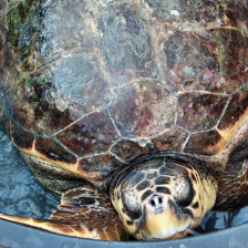
In fact, the answer is No since the model does not see any augmentations of the out-distribution samples in the training phase. To verify, we use t-SNE [42] to visualize the projected feature space of a ResNet-34 [15] supervisedly trained with CIFAR-10 [21] in Figure 1. The figure contains test samples from CIFAR-10 and SVHN [28] test sets. For each sample, we plot the raw feature and the feature of its augmented version with a line connecting them. It shows that the relative distance between a CIFAR-10 pair (red-blue pairs with black lines) is statistically smaller than that of an SVHN pair (green-orange pairs with gray lines). Similar observations widely exist across networks, datasets, and augmentation methods (see Appendix A). Therefore, a well-trained model is not robust towards augmentations of all distributions; Instead, the property only holds for in-distribution data.
Based on this observation, we develop our algorithm, named TTA-AD (Test Time Augmentation Anomaly Detection), which has the following characteristics:
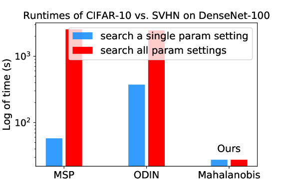
Performance. TTA-AD achieves comparable or better detection performance on challenging benchmark vision datasets for both supervised and unsupervised SOTA models. Efficiency. TTA-AD is a post-hoc algorithm which can be applied directly to a plain classifier. It only computes two forward passes to obtain the anomaly scores, which is far more efficient than most popular classifier-based algorithms. We provide a clock running time comparison in Figure 2. Prior-free. TTA-AD is dataset-agnostic and prior-free. So we do not have to tune the hyper-parameters with out-distribution prior, which may be hard or impossible to obtain during training. Adaptability. TTA-AD can not only help a plain classification model to detect anomalies, but also adapt to other representation learning anomaly detection methods [39]. Meanwhile, TTA-AD does not require access to internal features and gradients, which is desirable when a white box model is unavailable.
We further analyze the reasons for improved performance through empirical observations and theoretical analysis, which previous works often do not provide.
Empirically, TTA-AD gains benefits from mutual relations between different augmentations of a single sample. We name all the classes except for the maximum class as remaining classes. Specifically, we verify that the mutual relations between the remaining classes of a single sample’s different augmentations significantly differ for in- and out-distribution data. The idea is different from previous algorithms which focus on maximum probability [16, 25, 17], mutual relations between layers of a sample [34], mutual relations between different samples [39] and class-conditional distributions [24, 47]. Section 5.1 provides detailed evidence for the huge statistic difference of the remaining classes on in-distribution and out-distribution data.
Theoretically, anomaly detection is essentially a problem of sorting a binary sequence, where the two classes are drawn from in- and out-distributions. In this work, we provide theoretical analysis of TTA-AD’s success based on a theoretical tool named RUNS [44, 4], which evaluates the degree of confusion of a binary sequence in statistics. A detailed correlation between RUNS and the performance of TTA-AD is discussed in Section 5.2. Considering the strong connection between anomaly detection and RUNS, RUNS may serve as a theoretical tool in other anomaly detection works as well.
To conclude, our contributions are: 1) We observe the significant difference of the mutual relations for in- and out-distribution data and propose a new anomaly detection algorithm, TTA-AD, based on the observation. It achieves comparable or better results on challenging benchmark vision datasets for both supervised and unsupervised dataset-vs-dataset anomaly detection. 2) We provide both empirical and theoretical evidence to explain how TTA-AD works, which is not addressed by previous algorithms. 3) TTA-AD is more practical compared to the previous algorithms. Specifically, it is computationally efficient and free both to out-distribution prior and the model’s internal weights/gradients.
2 Related work
Dataset-vs-dataset anomaly detection
A series of previous works focus on the dataset-vs-dataset image classification setting. Hendrycks & Gimpel [16] observe that correctly classified samples tend to have larger maximum softmax probability, while erroneously classified and out-distribution samples have lower values. The distribution gap allows for the detecting anomalies. To enlarge the distribution gap, Hendrycks et al. [17] enhance the data representations by introducing self-supervised learning and Liang et al. [25] propose input pre-processing and temperature scaling. Input pre-processing advocates fine-tuning the input so that the model is more confident in its prediction. Temperature scaling introduces temperature to the softmax function. Besides maximum probability, Lee et al. [24] introduce the Mahalanobis score, which computes the class-conditional Gaussian distributions from a pre-trained model and confidence scores. Tack et al. [39] propose contrastive losses and a scoring function to improve anomaly detection performance on high-resolution images. Sastry & Oore [34] use Gram matrices of a single sample’s internal features from different layers.
Each of these classifier-based dataset level algorithms has their own characteristics. Prior out-distribution knowledge is required to tune the parameters by some algorithms [25, 24]. Although higher performance is reached, such prior knowledge is rare and unpredictable under certain scenes. Input pre-processing [18, 24, 25] is time-consuming because one needs several times of forwarding and backpropagation. Scoring-based methods are computationally costly since they rely on internal model features [1, 24, 34]. Our algorithm utilizes test time augmentation and consistency evaluation to achieve prior-free and computational friendly anomaly detection (summarized in Table 4).
Data augmentations in anomaly detection
Using data augmentations in anomaly detection has been applied by existing algorithms in both training and evaluating phases. Training data augmentation usually aims to learn a better data representation. Previous works employ augmentations from self-supervised learning and contrastive learning in training phase to gain better detection performance [17, 39, 50]. Test data augmentation usually relates to the calculation of anomaly scores. Golan & El-Yaniv utilize summarized predicted probability over multiple geometric augmentations at test time to detect anomalies [11]. Wang et al. calculate averaged negative entropy over each augmentation as the detection criterion [46].
Our TTA-AD uses test data augmentation as well but with two main differences. First, we utilize the relations between augmentations of a single sample, which is not explored by previous works. Second, we empirically verify that the performance improvement is attributed to the remaining classes, while previous works empirically find augmentations are helpful without any reasons.
Beyond the algorithms we mentioned above, various methods of anomaly detection are well summarized by Chalapathy & Chawla [6]. There are shallow methods such as OC-SVM [35], SVDD [40], Isolation Forest [27], and deep methods such as deep SVDD [32] and deep-SAD [33] used to detect anomalies under different anomaly settings. We also notice that model uncertainty is highly related to anomaly detection. In fact, anomaly detection is exactly a task that assigns uncertainty (or anomaly) scores to samples, so the final goals are similar. The main factor that distinguishes them is how such scores are generated [17, 36].
3 Data augmentation and consistency evaluation
We present our simple yet effective algorithm TTA-AD, which is purely based on test time data augmentation and consistency evaluation. The whole computation pipeline is shown in Algorithm 1.
Our algorithm adapts to both supervised and unsupervised pre-trained models. The performance in both cases is covered in experiments. Below, we first explain the two cores of our algorithm in detail.
3.1 Data augmentation and feature space distance
We use data augmentation techniques without backpropagation at test time, which is similar to TTA, to help enlarge the gap between in-distribution and out-distribution samples. Formally, given test data , a transformation function drawn from function space , the augmentation process can be described as . In our algorithm, the function space contains Fast Fourier Transformation (FFT) and Horizontal Flip (HF) because they satisfy the sensitivity criterion. Specifically, recent studies find that neural networks are less error-prone to low-frequency components [45], and deep neural networks and datasets are sensitive to visual chirality [26]. TTA-AD extends these conclusions by revealing that while the neural networks are known to be sensitive to high frequency components and visual chirality (horizontal flip), the sensitivity is enhanced in out-distribution data.
FFT is a widely used efficient image processing technique [5, 29]. FFT converts an image from the space domain to the frequency domain using a linear operator. Then the frequency representation can be inversely converted into the original image data by IFFT (Inverse Fast Fourier Transformation). In TTA-AD, we propose to cut off partial sensitive high-frequency signals. Our ablation study on the filter radius in Section 4.5 shows that the anomaly detection performance fluctuates little within a wide range of filter radius. In the following text, we will use to represent the FFT and IFFT transformation with a 100-pixel filter radius. Since discovering visual chirality [26], there have not been many studies exploring how to exploit the property. We introduce it into anomaly detection, and according to our observations, it indeed enlarges the distribution gap. We verify through extensive experiments (Figure 1 and Appendix A) to show that the sensitivity is more significant in out-distribution data with both transformations. Specifically, the distance of paired in-distribution sample features is statistically shorter than that of paired out-distribution samples. Our analysis in Section 5 further provides the empirical reasons and theoretical analysis.
Discussion
We note that there are also other transformations which may satisfy the sensitivity criterion such as adversarial examples. However, they may bring undesired randomness and high computation burden, which is contrary to the original intention of TTA-AD. Additionally, employing data augmentation is not a new idea in anomaly detection as mentioned in Section 2. Unlike previous algorithms, our algorithm focuses on the relationship between augmented feature pairs instead of treating each augmented output separately. We next illustrate the measurement of the mutual relationship in the following.
3.2 Consistency Evaluation
Unlike previous works that ignore the interaction between augmentations of a sample, our anomaly score evaluates the relations between augmentations of a single sample in a simple but effective form. With a model trained on the training (in-distribution) data, we denote the softmax output of as . Suppose we fix a transformation method . We define the consistency score of a given data as the inner product of the model output of and , which is .
To further enlarge the gap of the model output for in- and out-distribution data, we use a fixed temperature scaling technique. Given a sample , we denote the softmax output with temperature scaling parameter as . And, define our final anomaly score for a given sample as
| (1) |
Based on the observation (Figure 1), the model tends to make more consistent outputs for in-distribution data than out-distribution data. So should be close to for in-distribution data and should be approximately for out-distribution data. Such score assigning process is the basis of our theoretical analysis in Section 5.2.
4 Experiments
4.1 Compared algorithms and metrics
In anomaly detection, algorithms with different settings often cannot be measured simultaneously. For example, some algorithms focus on the one-class-vs-all setting [32, 11, 46, 12], while others focus on the dataset-vs-dataset setting [25, 50] only. There are also algorithms that cover multiple settings [17, 39]. Since our algorithm relies on the remaining classes, i.e. multiple classes in the training set, those one-vs-all algorithms are not compared. The SOTA algorithm of advanced dataset is CSI [39]. We also cover MSP [16], ODIN [25], Mahalanobis [24] and Rot [17].
Following previous works [17, 24, 39], we use the AUROC (Area Under Receiver Operating Characteristic curve) as our evaluation metric. It summarizes True Positive Rate (TPR) against False Positive Rate (FPR) at various threshold values. The use of the AUROC metric frees us from fixing a threshold and provides an overall comparison metric.
4.2 Dataset settings and classifier training
Dataset settings are diverse in anomaly detection. We mainly consider the advanced ImageNet [9] settings, including full set settings and two kinds of subset settings. We also verify on CIFAR [21] settings and put the results in Appendix I due to limited space.
In the full-size ImageNet setting, the whole validation set is treated as the in-distribution test set. Since the ImageNet training set already contains all-embracing natural scenery, the corresponding out-distribution dataset is chosen to be a publicly available artificial image dataset from Kaggle111https://www.kaggle.com/alamson/safebooru. We use the first 50000 figures since the ImageNet validation dataset is of the same size. Some examples of the dataset are depicted in Figure 7 in Appendix B. We will call this setting ImageNet vs. Artificial.
Additionally, two sources of subset settings are included. The ImageNet-30 subset setting is used in relevant researches [17, 39]. The corresponding out-distribution datasets includes CUB-200 [43], Stanford Dogs [20], Oxford Pets [30], Places-365 [49] with small images (256*256) validation set, Caltech-256 [14], and Describable Textures Dataset (DTD) [8]. Beyond that, we also validate our algorithm on several public ImageNet subset combinations introduced by other works [10, 41] and public sources222https://github.com/MadryLab/robustness.These additional three ImageNet subsets are Living 9, Geirhos 16, and Mixed 10. The out-distribution categories are randomly selected from the complement set. The detailed subset hierarchy and configuration are shown in Appendix B. In total, we consider four subset settings.
We notice the performance of anomaly detection is highly affected by the trained classifiers. So we train networks with three random seeds per setting and report the mean and variance. The training details are in Appendix H.
4.3 Detection results
This section covers the main anomaly detection results including the full ImageNet setting (Table 1) and four ImageNet subset settings (Table 2 and 3).
| Algorithm | Architecture | |
|---|---|---|
| ResNet-50 | DenseNet-121 | |
| MSP | ||
| Algorithm | Out-distribution dataset | AVG. | |||||
|---|---|---|---|---|---|---|---|
| CUB-200 | Dogs | Pets | Places | Caltech | DTD | ||
| Rot+Trans | |||||||
| CSI Unlabeled | |||||||
| (ours) | |||||||
| Architecture | Algorithm | ImageNet subset settings | ||
|---|---|---|---|---|
| Living 9 | Geirhos 16 | Mixed 10 | ||
| ResNet-50 | MSP | |||
| ODIN | ||||
| Mahalanobis1 | ||||
| DenseNet-121 | MSP | |||
| ODIN | ||||
| Mahalanobis2 | ||||
-
1,2
We use the official code and hyper parameter settings of the paper. The implementation details are in Appendix G.
ImageNet
For the full ImageNet vs. Artificial setting, we only compare our post-hoc TTA-AD with the MSP algorithm due to the computational costs of other algorithms being too large for the full size ImageNet. The performance is shown in Table 1.
ImageNet subsets
For ImageNet-30, we adapt the TTA-AD to the unsupervised CSI model by substituting the predicted probabilities in Eqn. (1) with output features (512 dimensional tensors). The results in Table 2 shows that a better average AUROC value is reached compared with Rot+Trans [17] and the SOTA algorithm, CSI [39], with designed scoring functions.
For the other three subset settings, Living 9, Geirhos 16, and Mixed 10, we compare TTA-AD with supervised algorithms listed in Table 3. We can see that TTA-AD is more efficient and outperforms all counterparts. All the compared algorithms are implemented according to the original paper and code except necessary modification of ImageNet figure size. Implementation details are stated in Appendix G.
Discussion
Zhou et al. [50] report that severe performance degradation of the Mahalanobis [24] exists when generalizing to other datasets due to validation bias. In order to verify whether TTA-AD also has similar problems, we conduct experiments on CIFAR-10 based settings to test the generalization ability of TTA-AD. Limited to space, the detection results are in Appendix I. Our experiments lead to a similar conclusion as Zhou et al. that simpler algorithms generalize better on different settings. The results also show that TTA-AD can not only achieve better results on advanced datasets, but also has stable generalization performance on low-resolution datasets.
| Algorithm |
|
|
|
|
||||||||
|---|---|---|---|---|---|---|---|---|---|---|---|---|
| ODIN [25] | Not Req. | Req. | Req. | 1FP+1BP+1FP | ||||||||
| Mahalanobis [24] | Req. | Req. | Req. |
|
||||||||
| TTA-AD (ours) | Not Req. | Not Req. | Not Req. | 2FP |
-
1
Compute feature mean and covariance of k selected layers.
-
2
Regression on the computed Mahalanobis score.
4.4 Algorithms running time
We show computational costs of all considered algorithms in this section since running time is important in practical use. We run all experiments on an RTX3090 graphics card. The post-hoc algorithms, ODIN and TTA-AD, do not include a training phase, while the Mahalanobis needs a little bit of time to train. All implementations are based on official code sources (See Appendix G). Figure 2 shows that TTA-AD only requires running time of advanced algorithms while maintaining comparable or better detection results (Table 3). The difference in running time is mainly due to the use of different techniques as summarized in Section 2 and Table 4. The number of parameter searching groups comes directly from the original papers and codes. The running time of CSI is missing because introducing contrastive learning is often considered much more time-inefficient than plain training which is the default training methods of the three algorithms in Figure 2. The details, criteria for choosing comparison algorithms and running times on other network architectures are stated in Appendix F.

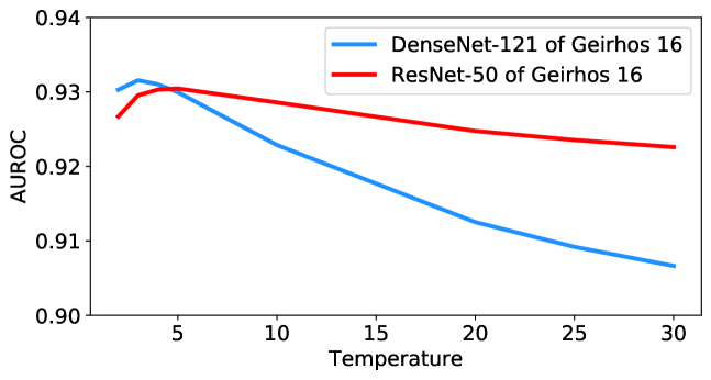
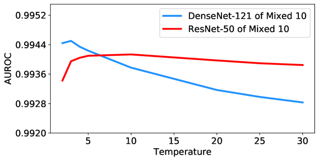
4.5 Ablation studies for filter radius and temperature
Performance tables in this paper include several different augmentation methods of TTA-AD. Although the AUROC values fluctuate with different augmentation methods and filter radius, the performance is similar. With linear searching across the FFT filter radius and temperature settings, we demonstrate that they have a small effect on the anomaly detection performance within a wide range.
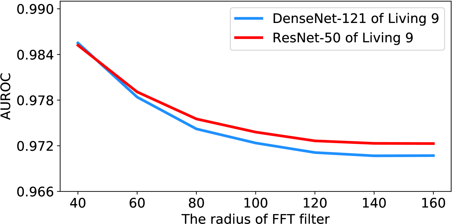
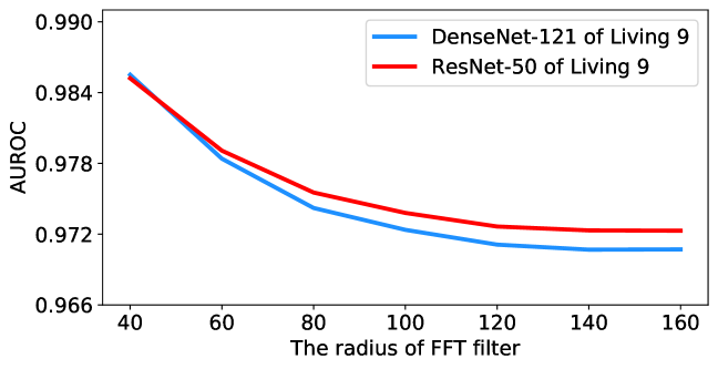
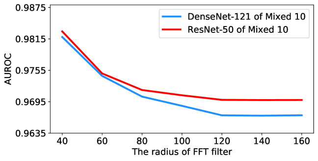
For the FFT filter radius, we provide ablation studies across a wide range of filter radius settings, ranging from 40 to 160 pixels, in Figure 4. Among all settings, TTA-AD does not degrade much and still outperforms other algorithms as shown in Table 3, which demonstrates that the performance of TTA-AD is not very sensitive to the filter radius. A possible reason is that the energy is highly concentrated in the low frequency space instead of high frequency parts. More ablations of other settings are in Appendix J.
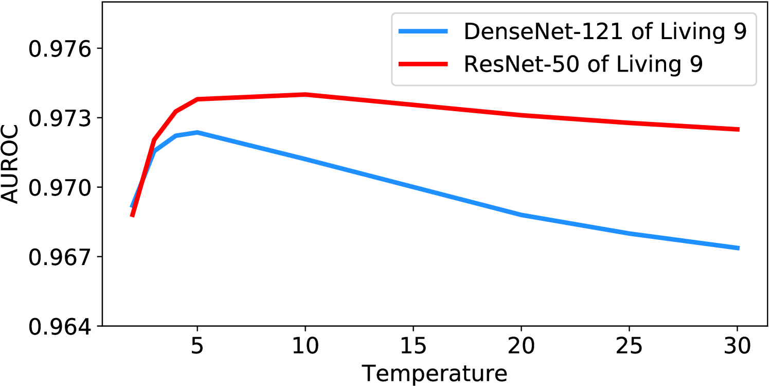
Unlike the previous algorithms [24, 25], which consider large-scale candidates of temperature scaling (e.g., from 1 to 1000) and then do the grid-search with prior out-distribution knowledge, we empirically find that the best temperature for our method is stable around 5 and the performance does not decrease much within the considered wide temperature range. All our experiments set the temperature parameter to 5 if not specified. Ablation studies for temperature parameter are shown in Figure 4, and more results can be found in Appendix K. All curves show that TTA-AD is not sensitive to the temperature parameter, thus we do not have to tune it with out-distribution prior.
5 Algorithm analysis
In this section, we will explain why data augmentation and consistency evaluation help to detect anomalies empirically (Section 5.1) and mathematically (Section 5.2).
5.1 Empirical analysis of using remaining classes probability
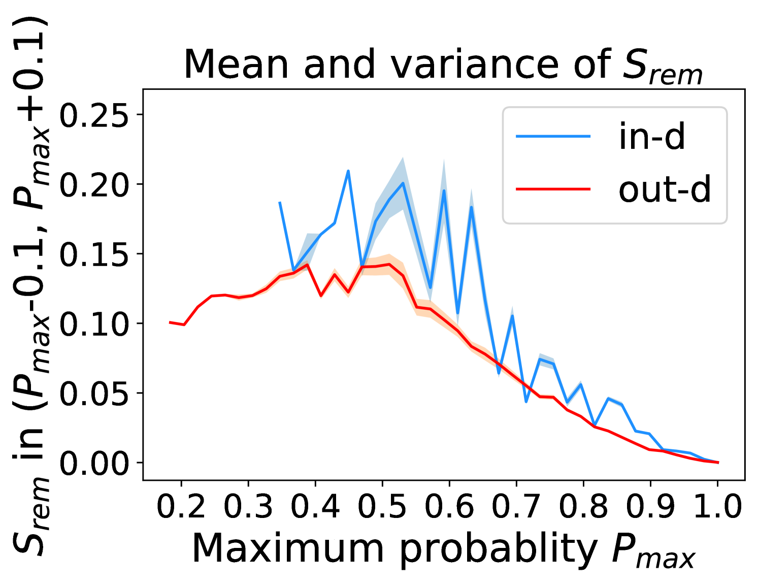
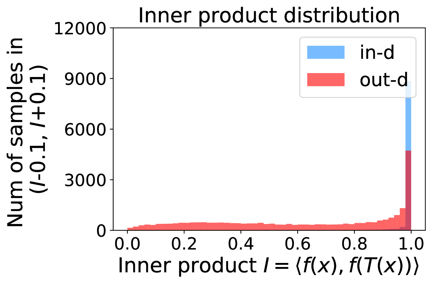
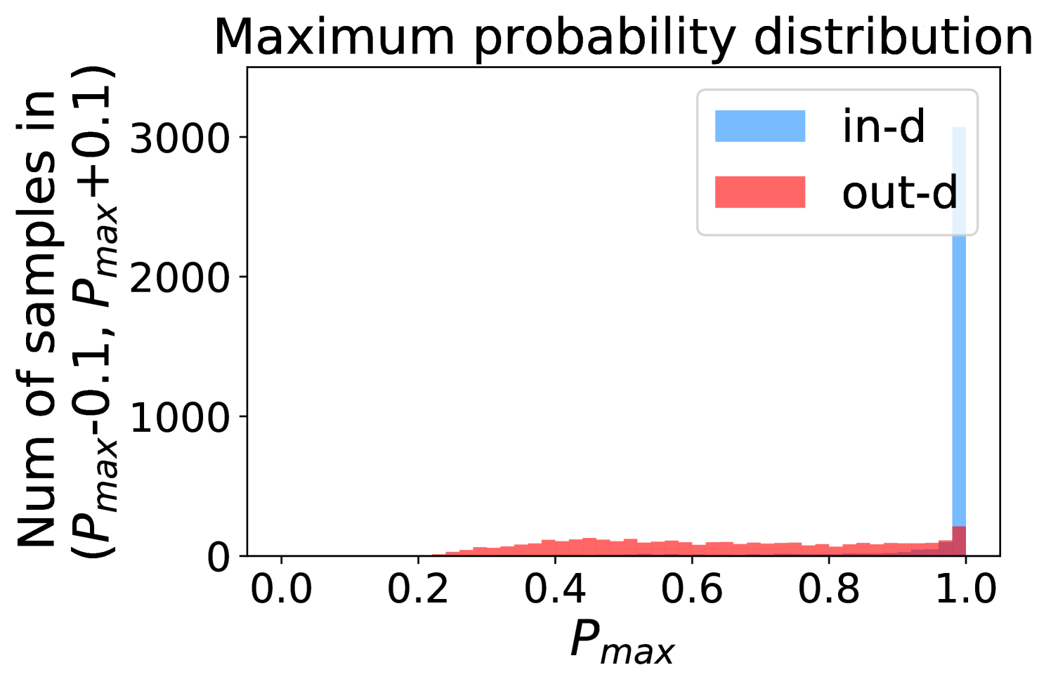
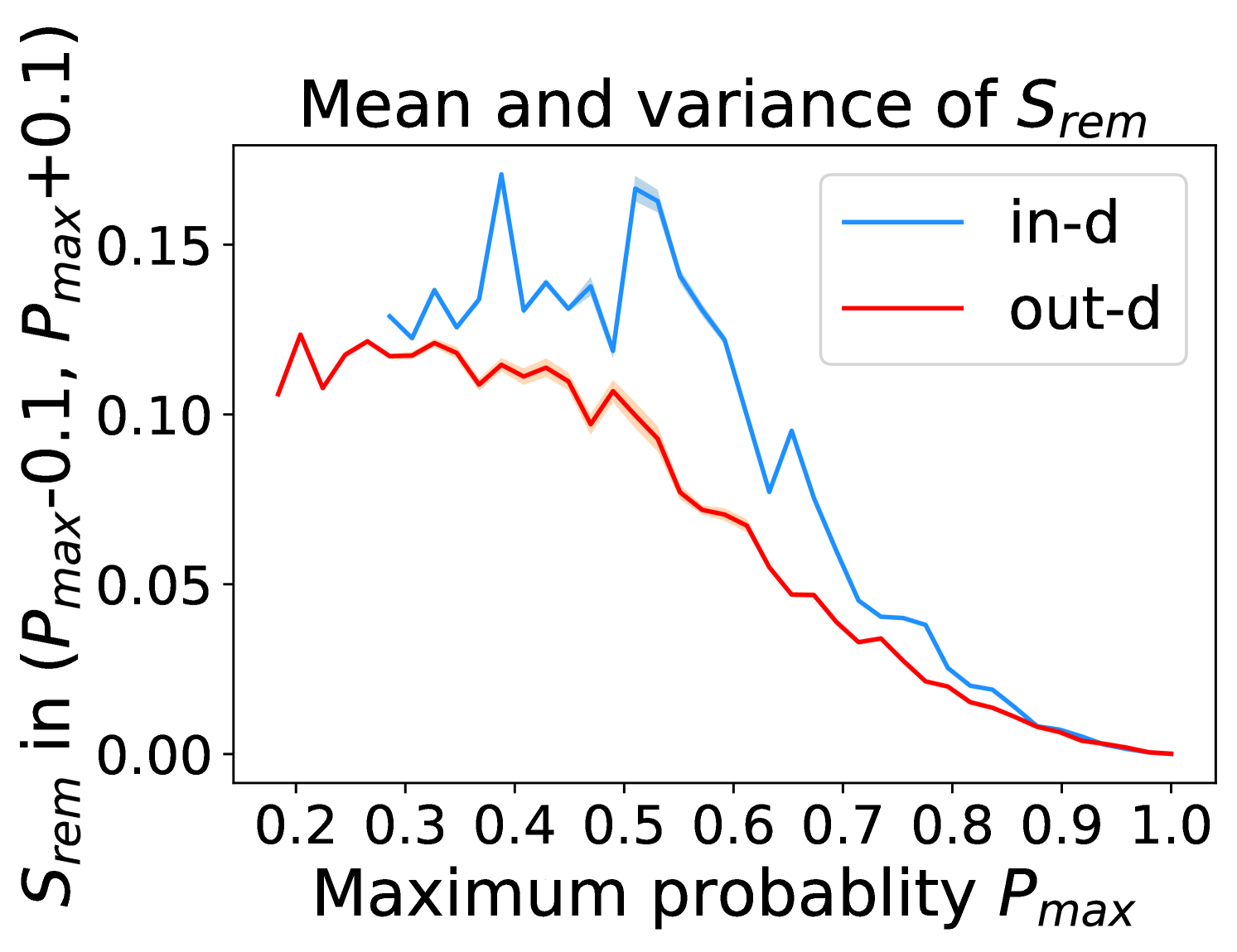
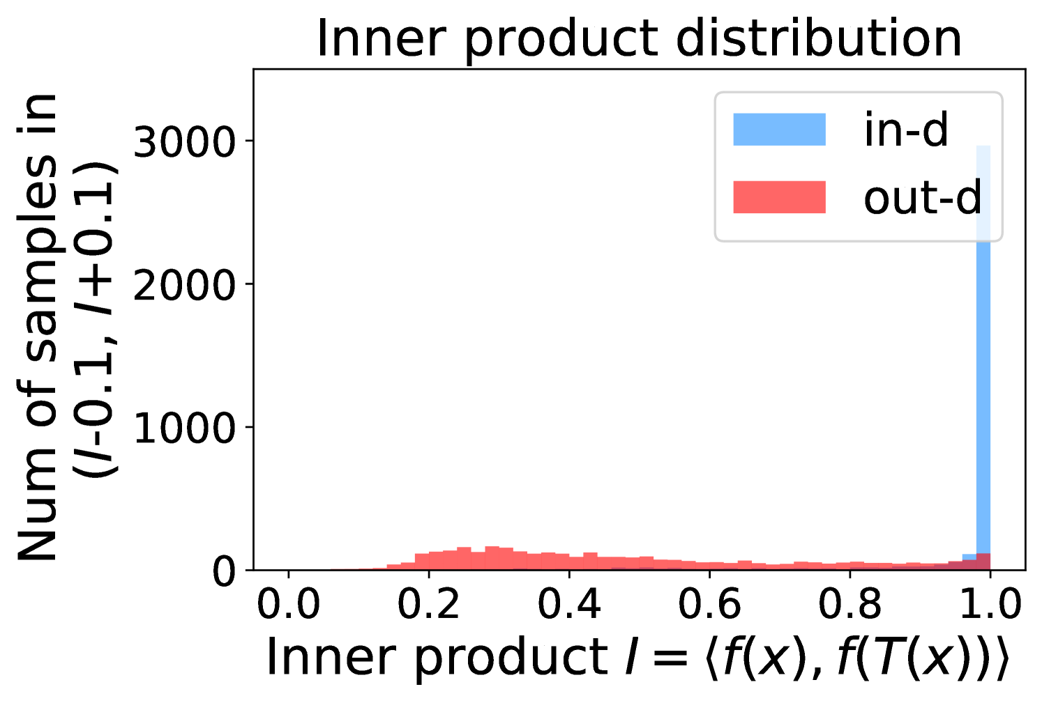
Our anomaly score (Eqn (1)) adds up all class probabilities rather than focusing only on the maximum predicted probability [16, 17]. The main difference between consistency evaluation and maximum predicted probability comes from the remaining score , defined as
| (2) |
where is the predicted class with the highest probability of the input .
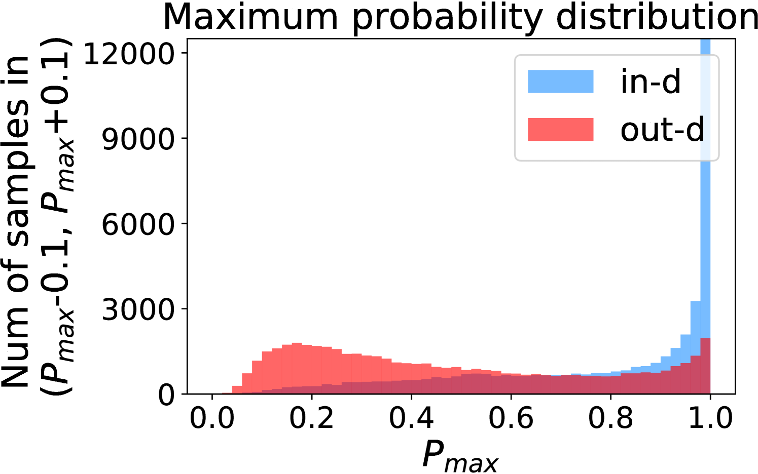
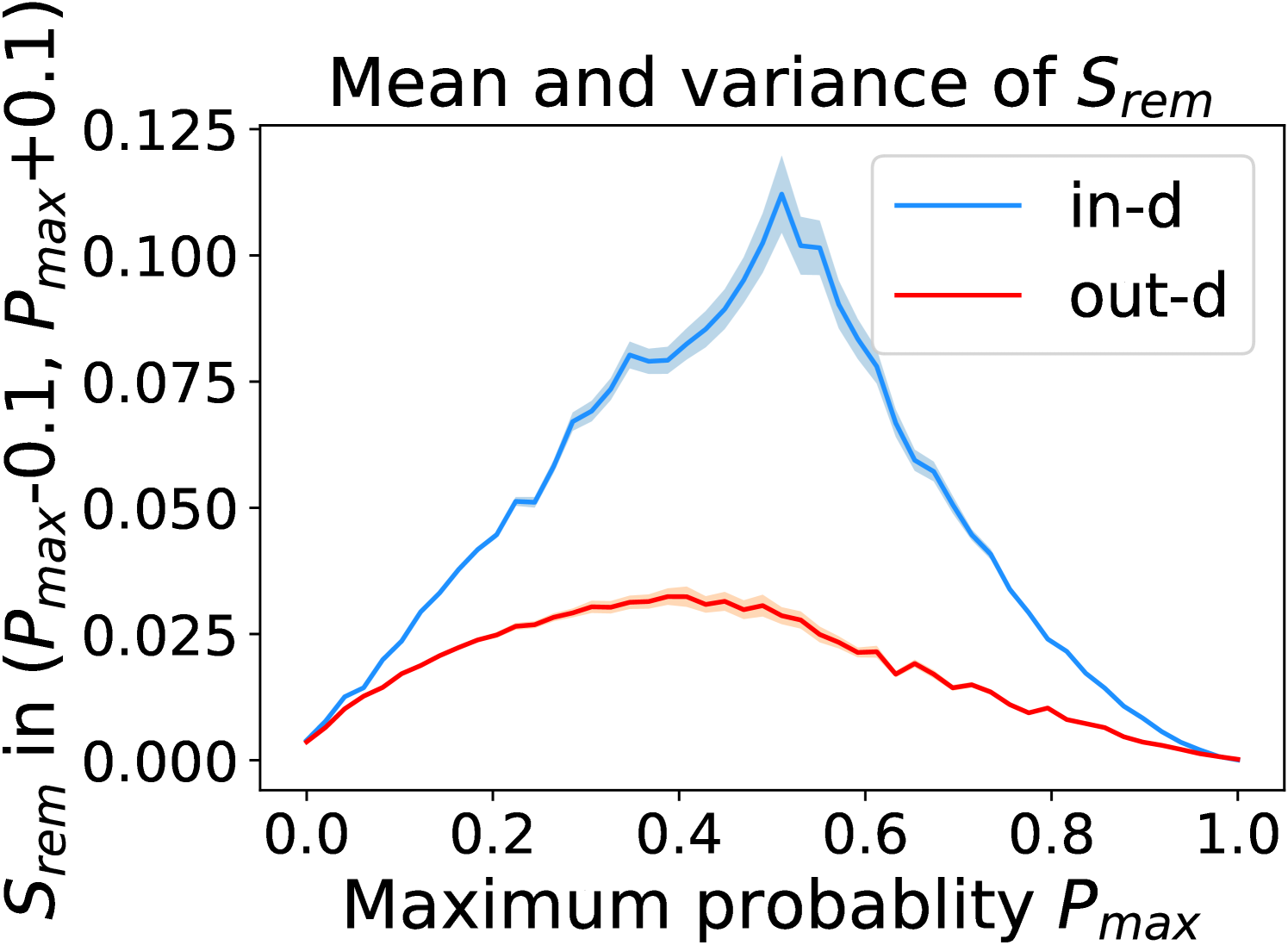
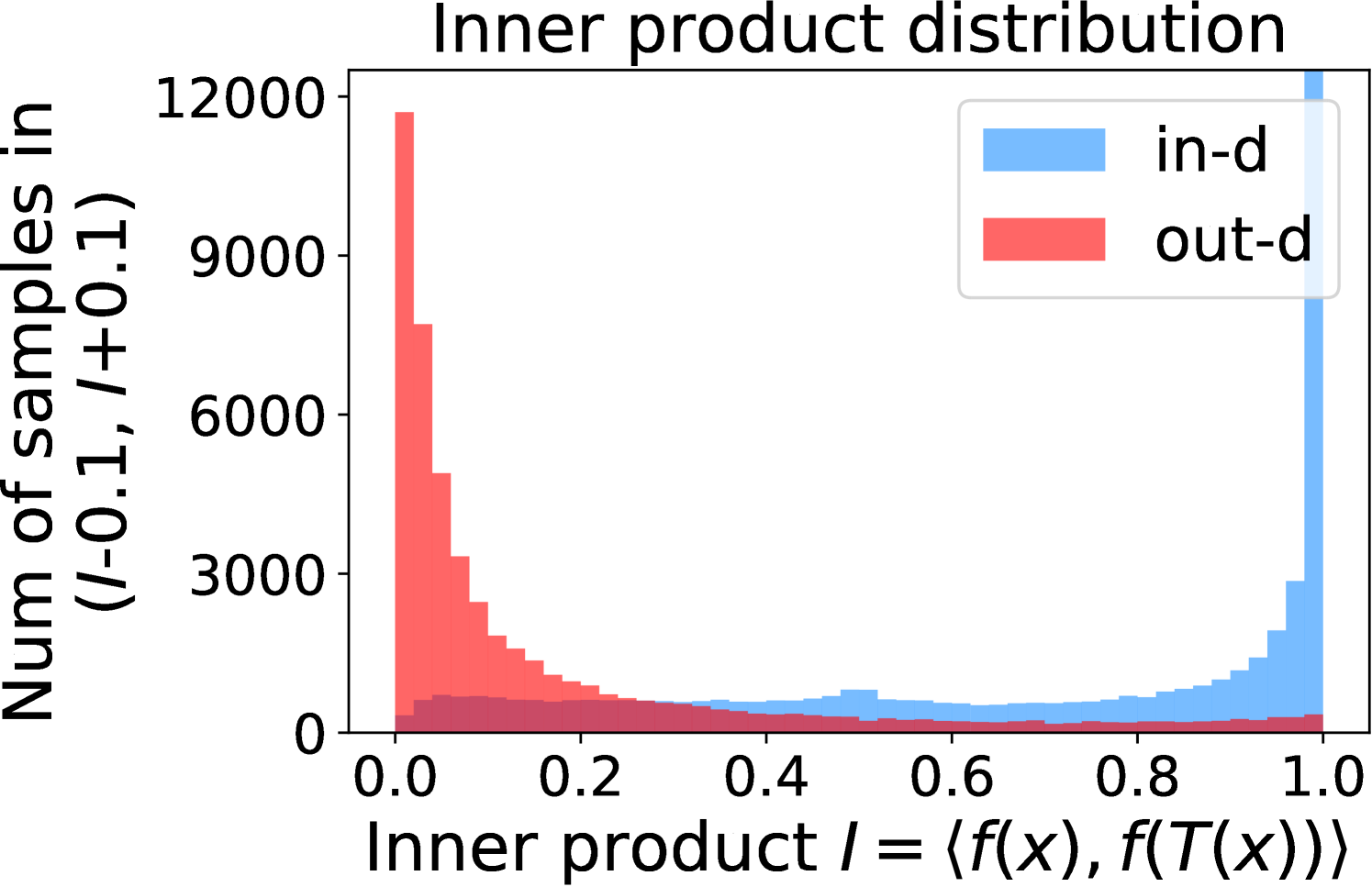
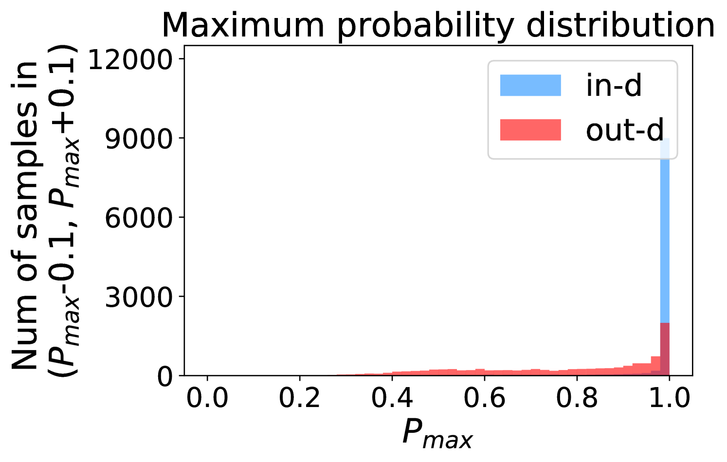
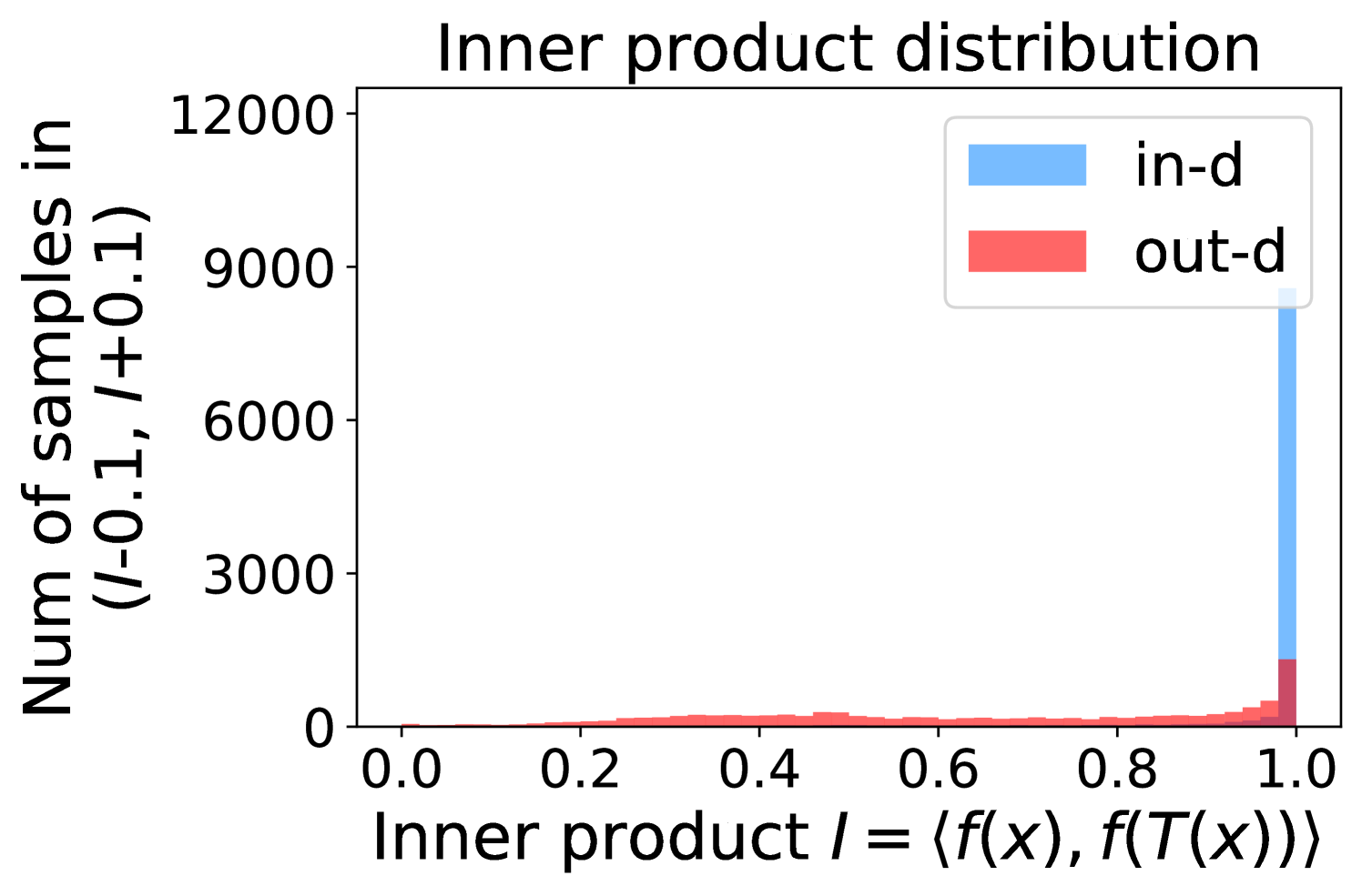
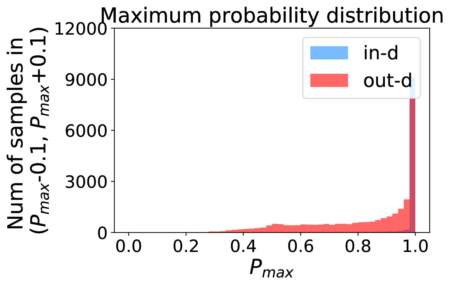
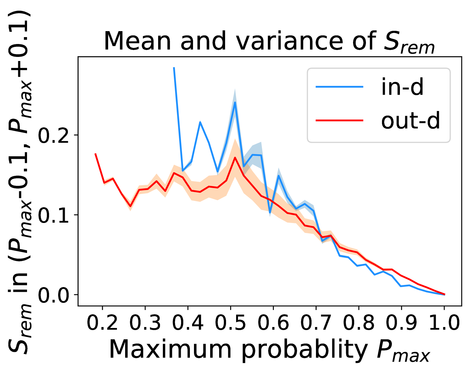
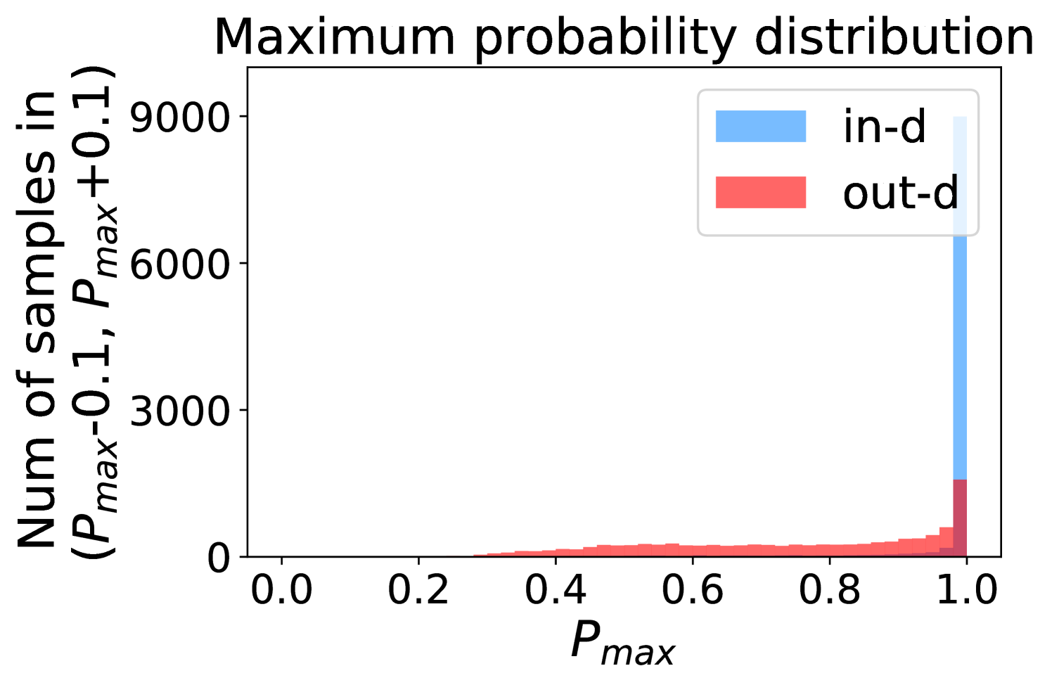
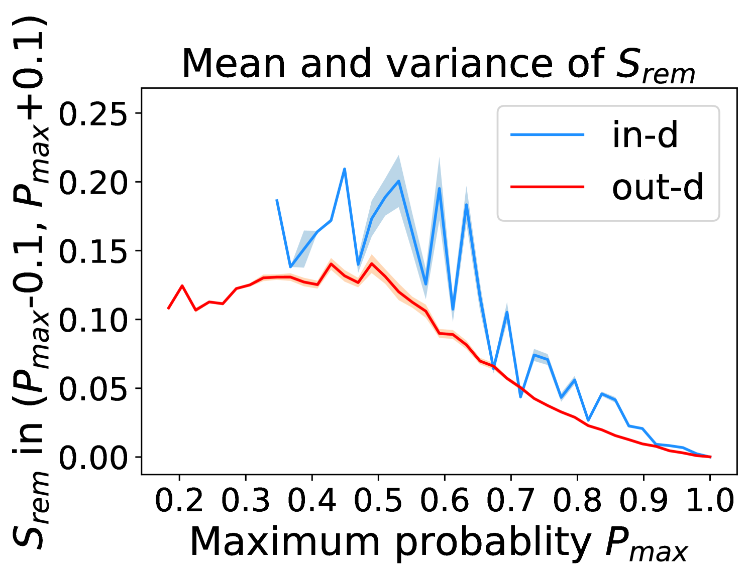
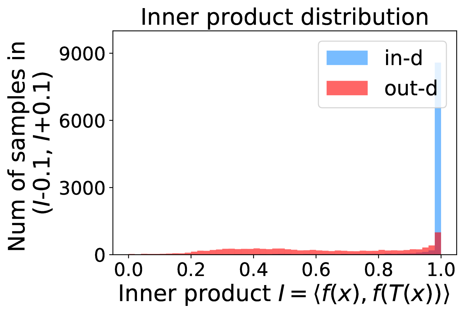
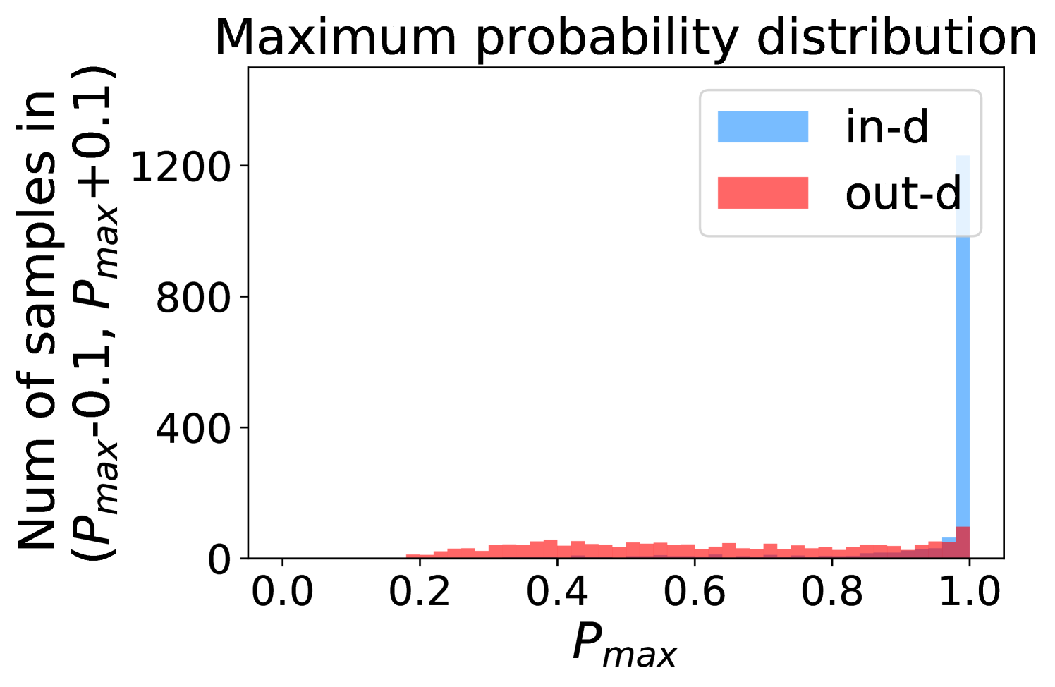
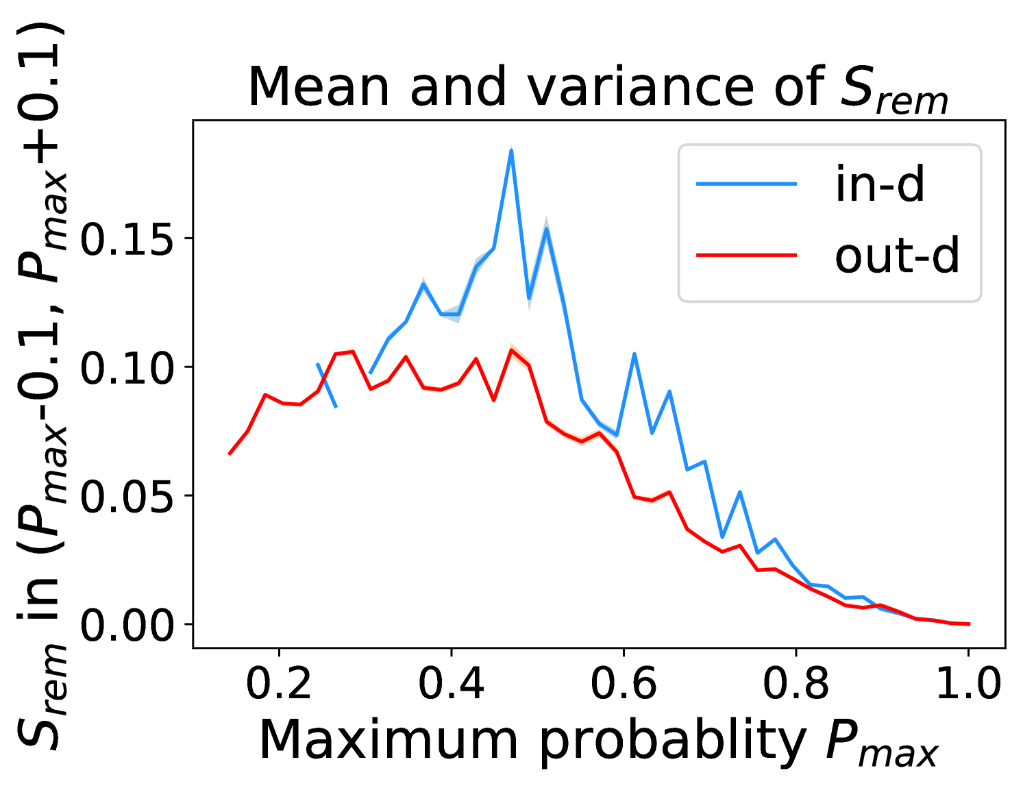
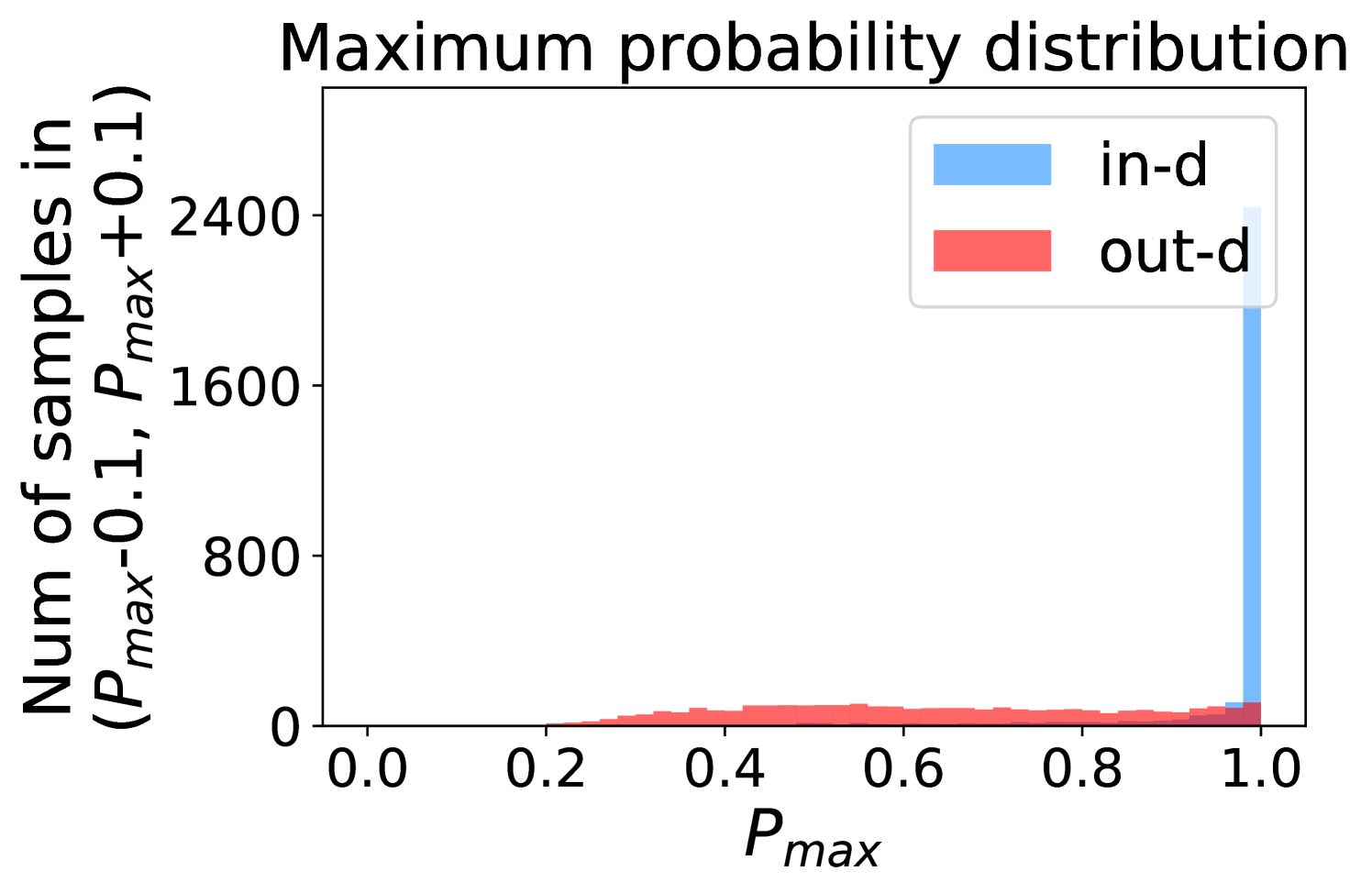
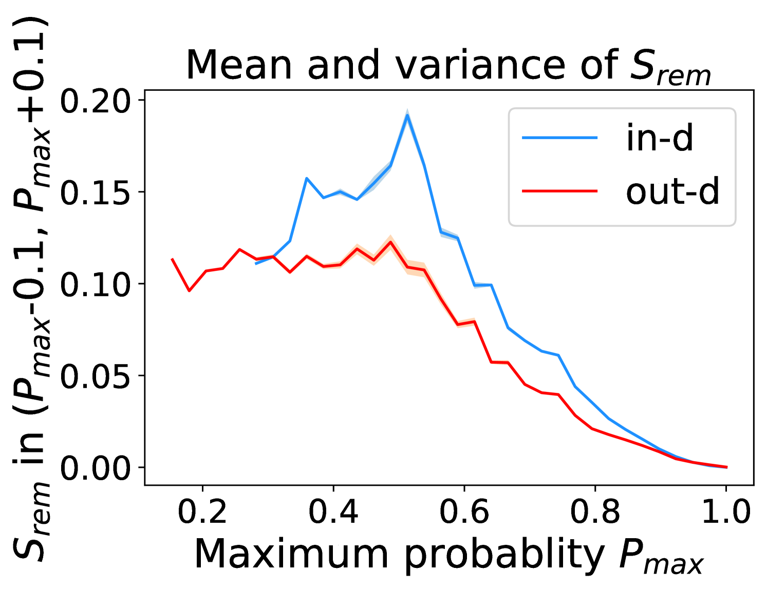
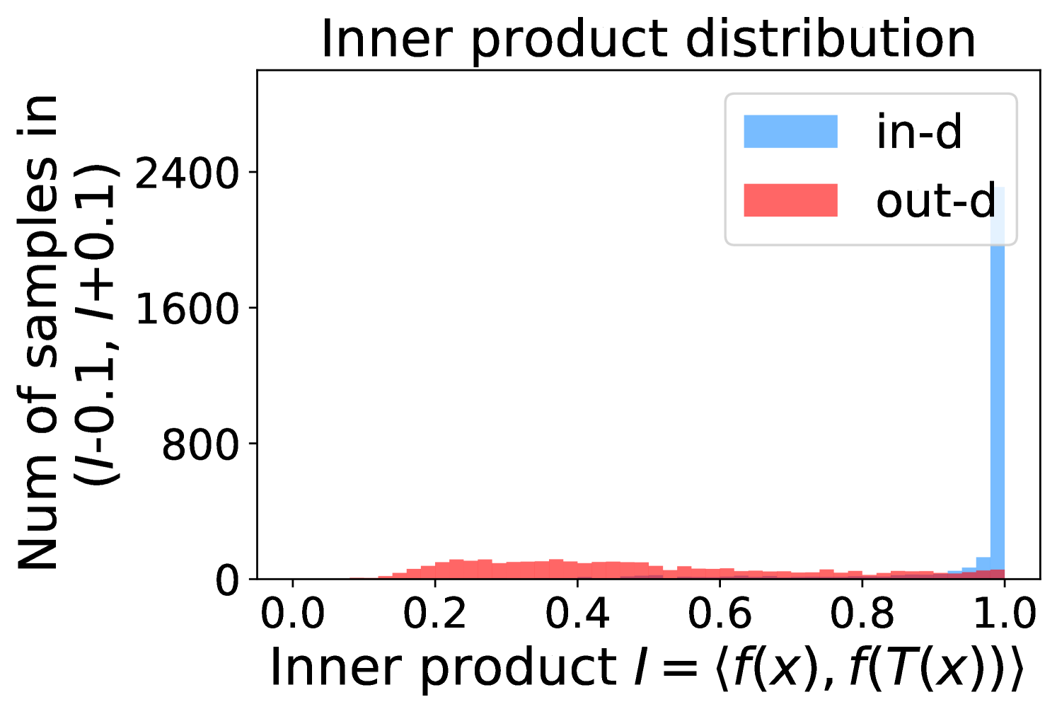
Figure 5 shows the beneficial effect of the remaining classes. First, Figure 5(a) presents the distribution of maximum probability. Then, we calculate the mean and variance of the remaining scores in each evenly divided interval, as Figure 5(b) shows. To draw the Figure 5(b), we first evenly divide the interval in Figure 5(a) into 50 parts. Then we pick one interval , select all the samples whose maximum predicted probability is between , and compute the mean and variance of those selected samples’ remaining scores . For every interval, we process the in- and out-distribution data separately indicated by the red and blue lines.
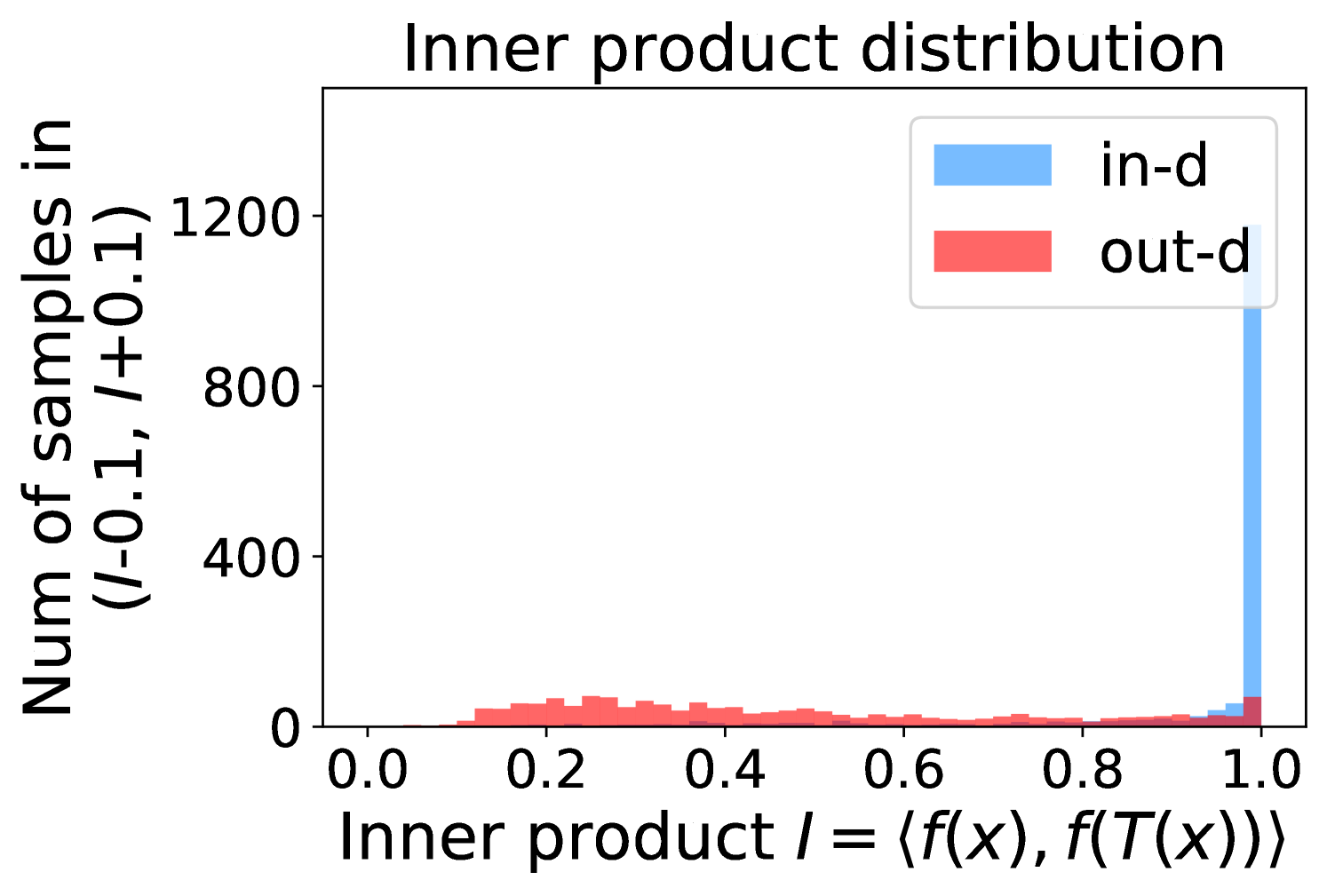
Intuitively, samples from both in- and out-distributions with similar values are mixed within one same interval (Figure 5(a)). Figure 5(b) shows that for samples within the same interval, the remaining scores of the in-distribution samples are statistically larger than that of out-distribution samples. Therefore, adding the remaining scores to the data within the same interval in Figure 5(a) makes the in- and out-distribution samples distinguishable. When this process happens in each interval, we obtain our inner product scores () as depicted in Figure 5(c), which improves the maximum probability method from Figure 5(a).
Comparing the maximum probability (Figure 5(a)) and consistency evaluation methods (Figure 5(c)), our method is more discriminative. Generally, a larger gap in Figure 5(b) indicates a higher performance improvement. This empirical analysis is consistent with our numerical results in Section 4. Similar observations across network architectures and datasets can be found in Appendix C.
5.2 Theoretical analysis based on runs
The most fundamental and common part of anomaly detection is attaching a real-valued score calculated by the algorithm to each sample. We then obtain a sequence by sorting all samples according to their scores from small to large. If we label the out- and in-distribution samples as 0 and 1, respectively, we will finally get a mixing binary sequence. Intuitively, a sequence with good sorting (like ) is preferred, but how to quantitatively describe the mixing degree? Empirically, we use AUROC but its discontinuity hinders the development of anomaly detection theory. To analyze our algorithm, we propose to use expected runs [44, 4] as a continuous surrogate to approximately measure the confusion degree of a binary sequence:
Definition 5.1 (Runs).
The runs number of a binary sequence is the number of maximal non-empty segments consisting of adjacent equal elements. Each segment is called a run.
For example, the sequence has 5 runs. Ideally, the in-distribution and out-distribution samples are completely separable ( ), so the runs number is 2. On the contrary, the runs number of the worst case, when the two kinds of samples alternate in the sequence, equals the sequence length.
Assume the in-distribution and out-distribution sample scores are drawn from two distributions. Then the expected runs number evaluates the similarity of the two distributions. The above two examples suggest that more separable distributions lead to a smaller expected runs number. Now we show how to calculate the expected runs number for any given two distributions in Lemma 5.2.
Lemma 5.2 (Calculation of the expected runs number).
Consider two random variables with PDF and with PDF . Assume for , , and the length of the support is upper bounded by . We assume the first-order derivative is bounded by , namely and . Then, for samples from distribution and samples from distribution , if while , we have
In the rest of the paper, we only consider the integral term while ignoring the little term.
We will derive a sufficient condition based on the expected runs number to identify our algorithm’s effectiveness. The supports of and are . Considering the two distributions in real datasets (see Figure 10 in Appendix D.3), we model the two distributions as Beta distributions and denote the runs number as . Lemma 5.3 investigates how the Beta distribution parameters increases/decreases the expected runs number.
Lemma 5.3 (Runs number increases/decreases).
When , we have . When , we have . By symmetry, performs similarly.
For example, when , we see . We leave the necessary and sufficient conditions for future work. Limited to space, we put the detailed proof and statements in Appendix D.
More generally, the expected runs provides a general theoretical surrogate for anomaly detection. In order to analyze the pros and cons of the algorithm performance, we can model the distribution of anomaly scores of in- and out-distribution, compute the runs, and derive runs with respect to distribution parameters. This will let us know how the distributions affect the runs number, which may guide designing and tuning the algorithms.
6 Limitation
Although TTA-AD is effective and easy to be implemented, it has its inherit limitations. TTA-AD may fail under some adversarially designed synthetic datasets, e.g., a transformation-invariant vision dataset. Additionally, the goal of proposing runs based theoretical analysis is to reduce the gap between theoretical analysis and practical metrics of anomaly detection. There is still some future work to refine this theoretical framework.
7 Conclusion
In this paper, we propose a simple yet effective dataset-vs-dataset vision post-hoc anomaly detection algorithm TTA-AD, which reaches comparable or better detection performance with current advanced and SOTA algorithms. It largely reduces the computational costs, demands no specific network architectures, no access to the internal feature, and no prior out-distribution data knowledge. We empirically show that TTA-AD gains performance improvement from the remaining classes, which are ignored by some previous works. Meanwhile, we provide a general theoretical framework based on runs to serve as a surrogate for reducing the gap between theoretical analysis and practical applications in anomaly detection.
References
- [1] Vahdat Abdelzad, Krzysztof Czarnecki, Rick Salay, Taylor Denouden, Sachin Vernekar, and Buu Phan. Detecting out-of-distribution inputs in deep neural networks using an early-layer output. CoRR, abs/1910.10307, 2019.
- [2] Charu C. Aggarwal. Outlier Analysis. Springer, 2013.
- [3] Dario Amodei, Chris Olah, Jacob Steinhardt, Paul F. Christiano, John Schulman, and Dan Mané. Concrete problems in AI safety. CoRR, abs/1606.06565, 2016.
- [4] DE Barton and FN David. Multiple runs. Biometrika, 44(1/2):168–178, 1957.
- [5] Ronald Newbold Bracewell and Ronald N Bracewell. The Fourier transform and its applications, volume 31999. McGraw-Hill New York, 1986.
- [6] Raghavendra Chalapathy and Sanjay Chawla. Deep learning for anomaly detection: A survey. CoRR, abs/1901.03407, 2019.
- [7] Ting Chen, Simon Kornblith, Mohammad Norouzi, and Geoffrey E. Hinton. A simple framework for contrastive learning of visual representations. CoRR, abs/2002.05709, 2020.
- [8] Mircea Cimpoi, Subhransu Maji, Iasonas Kokkinos, Sammy Mohamed, and Andrea Vedaldi. Describing textures in the wild. In Proceedings of the IEEE Conference on Computer Vision and Pattern Recognition, pages 3606–3613, 2014.
- [9] Jia Deng, Wei Dong, Richard Socher, Li-Jia Li, Kai Li, and Li Fei-Fei. Imagenet: A large-scale hierarchical image database. In CVPR 2009. IEEE, 2009.
- [10] Robert Geirhos, Patricia Rubisch, Claudio Michaelis, Matthias Bethge, Felix A. Wichmann, and Wieland Brendel. Imagenet-trained cnns are biased towards texture; increasing shape bias improves accuracy and robustness. In ICLR 2019, 2019.
- [11] Izhak Golan and Ran El-Yaniv. Deep anomaly detection using geometric transformations. In NeurIPS 2018, 2018.
- [12] Dong Gong, Lingqiao Liu, Vuong Le, Budhaditya Saha, Moussa Reda Mansour, Svetha Venkatesh, and Anton van den Hengel. Memorizing normality to detect anomaly: Memory-augmented deep autoencoder for unsupervised anomaly detection. In ICCV 2019. IEEE, 2019.
- [13] Ian J. Goodfellow, Jonathon Shlens, and Christian Szegedy. Explaining and harnessing adversarial examples. In ICLR 2015, 2015.
- [14] Gregory Griffin, Alex Holub, and Pietro Perona. Caltech-256 object category dataset. 2007.
- [15] Kaiming He, Xiangyu Zhang, Shaoqing Ren, and Jian Sun. Deep residual learning for image recognition. In CVPR 2016, 2016.
- [16] Dan Hendrycks and Kevin Gimpel. A baseline for detecting misclassified and out-of-distribution examples in neural networks. In ICLR 2017, 2017.
- [17] Dan Hendrycks, Mantas Mazeika, Saurav Kadavath, and Dawn Song. Using self-supervised learning can improve model robustness and uncertainty. In NeurIPS 2019, 2019.
- [18] Yen-Chang Hsu, Yilin Shen, Hongxia Jin, and Zsolt Kira. Generalized ODIN: detecting out-of-distribution image without learning from out-of-distribution data. In CVPR 2020, 2020.
- [19] Gao Huang, Zhuang Liu, Laurens van der Maaten, and Kilian Q. Weinberger. Densely connected convolutional networks. In CVPR 2017, 2017.
- [20] Aditya Khosla, Nityananda Jayadevaprakash, Bangpeng Yao, and Fei-Fei Li. Novel dataset for fine-grained image categorization: Stanford dogs. In Proc. CVPR Workshop on Fine-Grained Visual Categorization (FGVC), volume 2. Citeseer, 2011.
- [21] Alex Krizhevsky, Geoffrey Hinton, et al. Learning multiple layers of features from tiny images. 2009.
- [22] Ya Le and Xuan Yang. Tiny imagenet visual recognition challenge. CS 231N, 7(7):3, 2015.
- [23] Yann LeCun, Yoshua Bengio, and Geoffrey E. Hinton. Deep learning. Nat., 521(7553):436–444, 2015.
- [24] Kimin Lee, Kibok Lee, Honglak Lee, and Jinwoo Shin. A simple unified framework for detecting out-of-distribution samples and adversarial attacks. In NeurIPS 2018, 2018.
- [25] Shiyu Liang, Yixuan Li, and R. Srikant. Enhancing the reliability of out-of-distribution image detection in neural networks. In ICLR 2018, 2018.
- [26] Zhiqiu Lin, Jin Sun, Abe Davis, and Noah Snavely. Visual chirality. In Proceedings of the IEEE/CVF Conference on Computer Vision and Pattern Recognition, pages 12295–12303, 2020.
- [27] Fei Tony Liu, Kai Ming Ting, and Zhi-Hua Zhou. Isolation forest. In ICDM 2008, 2008.
- [28] Yuval Netzer, Tao Wang, Adam Coates, Alessandro Bissacco, Bo Wu, and Andrew Y Ng. Reading digits in natural images with unsupervised feature learning. 2011.
- [29] A.V. Oppenheim, A.S. Willsky, S.H. Nawab, with Hamid, and I.T. Young. Signals & Systems. Prentice-Hall signal processing series. Prentice Hall, 1997.
- [30] Omkar M Parkhi, Andrea Vedaldi, Andrew Zisserman, and CV Jawahar. Cats and dogs. In CVPR 2012, 2012.
- [31] Adam Paszke, Sam Gross, Francisco Massa, Adam Lerer, James Bradbury, Gregory Chanan, Trevor Killeen, Zeming Lin, Natalia Gimelshein, Luca Antiga, Alban Desmaison, Andreas Kopf, Edward Yang, Zachary DeVito, Martin Raison, Alykhan Tejani, Sasank Chilamkurthy, Benoit Steiner, Lu Fang, Junjie Bai, and Soumith Chintala. Pytorch: An imperative style, high-performance deep learning library. In NeurIPS 2019. 2019.
- [32] Lukas Ruff, Nico Görnitz, Lucas Deecke, Shoaib Ahmed Siddiqui, Robert A. Vandermeulen, Alexander Binder, Emmanuel Müller, and Marius Kloft. Deep one-class classification. In ICML 2018, 2018.
- [33] Lukas Ruff, Robert A. Vandermeulen, Nico Görnitz, Alexander Binder, Emmanuel Müller, Klaus-Robert Müller, and Marius Kloft. Deep semi-supervised anomaly detection. In ICLR 2020, 2020.
- [34] Chandramouli Shama Sastry and Sageev Oore. Detecting out-of-distribution examples with gram matrices. In International Conference on Machine Learning, pages 8491–8501. PMLR, 2020.
- [35] Bernhard Schölkopf, Robert C. Williamson, Alexander J. Smola, John Shawe-Taylor, and John C. Platt. Support vector method for novelty detection. In NeurIPS 1999, 1999.
- [36] Philipp Seeböck, José Ignacio Orlando, Thomas Schlegl, Sebastian M. Waldstein, Hrvoje Bogunovic, Sophie Klimscha, Georg Langs, and Ursula Schmidt-Erfurth. Exploiting epistemic uncertainty of anatomy segmentation for anomaly detection in retinal OCT. IEEE Trans. Medical Imaging, 39(1):87–98, 2020.
- [37] Divya Shanmugam, Davis W. Blalock, Guha Balakrishnan, and John V. Guttag. When and why test-time augmentation works. CoRR, abs/2011.11156, 2020.
- [38] Connor Shorten and Taghi M. Khoshgoftaar. A survey on image data augmentation for deep learning. J. Big Data, 6:60, 2019.
- [39] Jihoon Tack, Sangwoo Mo, Jongheon Jeong, and Jinwoo Shin. CSI: novelty detection via contrastive learning on distributionally shifted instances. In Hugo Larochelle, Marc’Aurelio Ranzato, Raia Hadsell, Maria-Florina Balcan, and Hsuan-Tien Lin, editors, Advances in Neural Information Processing Systems 33: Annual Conference on Neural Information Processing Systems 2020, NeurIPS 2020, December 6-12, 2020, virtual, 2020.
- [40] David M. J. Tax and Robert P. W. Duin. Support vector data description. Mach. Learn., 54(1):45–66, 2004.
- [41] Dimitris Tsipras, Shibani Santurkar, Logan Engstrom, Andrew Ilyas, and Aleksander Madry. From imagenet to image classification: Contextualizing progress on benchmarks. CoRR, abs/2005.11295, 2020.
- [42] Laurens Van der Maaten and Geoffrey Hinton. Visualizing data using t-sne. Journal of machine learning research, 9(11), 2008.
- [43] C. Wah, S. Branson, P. Welinder, P. Perona, and S. Belongie. The Caltech-UCSD Birds-200-2011 Dataset. Technical Report CNS-TR-2011-001, California Institute of Technology, 2011.
- [44] Abraham Wald and Jacob Wolfowitz. On a test whether two samples are from the same population. The Annals of Mathematical Statistics, 11(2):147–162, 1940.
- [45] Haohan Wang, Xindi Wu, Zeyi Huang, and Eric P. Xing. High-frequency component helps explain the generalization of convolutional neural networks. In CVPR 2020, 2020.
- [46] Siqi Wang, Yijie Zeng, Xinwang Liu, En Zhu, Jianping Yin, Chuanfu Xu, and Marius Kloft. Effective end-to-end unsupervised outlier detection via inlier priority of discriminative network. In NeurIPS 2019, 2019.
- [47] Jim Winkens, Rudy Bunel, Abhijit Guha Roy, Robert Stanforth, Vivek Natarajan, Joseph R Ledsam, Patricia MacWilliams, Pushmeet Kohli, Alan Karthikesalingam, Simon Kohl, et al. Contrastive training for improved out-of-distribution detection. arXiv preprint arXiv:2007.05566, 2020.
- [48] Fisher Yu, Ari Seff, Yinda Zhang, Shuran Song, Thomas Funkhouser, and Jianxiong Xiao. Lsun: Construction of a large-scale image dataset using deep learning with humans in the loop. arXiv preprint arXiv:1506.03365, 2015.
- [49] Bolei Zhou, Àgata Lapedriza, Aditya Khosla, Aude Oliva, and Antonio Torralba. Places: A 10 million image database for scene recognition. IEEE Trans. Pattern Anal. Mach. Intell., 2018.
- [50] Zhi Zhou, Lan-Zhe Guo, Zhanzhan Cheng, Yu-Feng Li, and Shiliang Pu. Step: Out-of-distribution detection in the presence of limited in-distribution labeled data. Advances in Neural Information Processing Systems, 34, 2021.
Checklist
-
1.
For all authors…
-
(a)
Do the main claims made in the abstract and introduction accurately reflect the paper’s contributions and scope? [Yes]
-
(b)
Did you describe the limitations of your work? [Yes] See Section 6.
-
(c)
Did you discuss any potential negative societal impacts of your work? [N/A]
-
(d)
Have you read the ethics review guidelines and ensured that your paper conforms to them? [Yes]
-
(a)
- 2.
-
3.
If you ran experiments…
-
(a)
Did you include the code, data, and instructions needed to reproduce the main experimental results (either in the supplemental material or as a URL)? [Yes] See Appendix G.
-
(b)
Did you specify all the training details (e.g., data splits, hyperparameters, how they were chosen)? [Yes] See Appendix G.
-
(c)
Did you report error bars (e.g., with respect to the random seed after running experiments multiple times)? [Yes] Results are reported with mean and variance.
-
(d)
Did you include the total amount of compute and the type of resources used (e.g., type of GPUs, internal cluster, or cloud provider)? [Yes] See Section 4.4.
-
(a)
-
4.
If you are using existing assets (e.g., code, data, models) or curating/releasing new assets…
-
(a)
If your work uses existing assets, did you cite the creators? [Yes]
-
(b)
Did you mention the license of the assets? [Yes]
-
(c)
Did you include any new assets either in the supplemental material or as a URL? [N/A]
-
(d)
Did you discuss whether and how consent was obtained from people whose data you’re using/curating? [N/A]
-
(e)
Did you discuss whether the data you are using/curating contains personally identifiable information or offensive content? [N/A]
-
(a)
-
5.
If you used crowdsourcing or conducted research with human subjects…
-
(a)
Did you include the full text of instructions given to participants and screenshots, if applicable? [N/A]
-
(b)
Did you describe any potential participant risks, with links to Institutional Review Board (IRB) approvals, if applicable? [N/A]
-
(c)
Did you include the estimated hourly wage paid to participants and the total amount spent on participant compensation? [N/A]
-
(a)
Appendix A Test time augmentation feature space under different data distributions
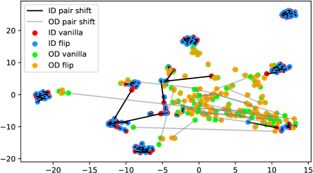
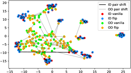
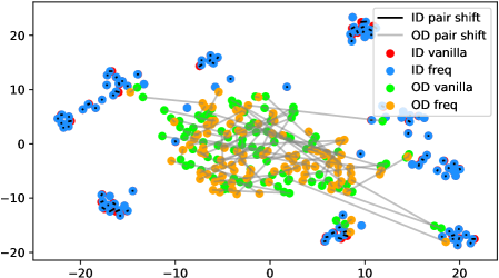
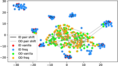
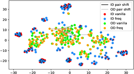
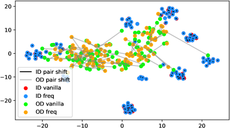
We verify the observation mentioned in Section 1 across architectures, dataset settings, and augmentation methods in Figure 6. Due to the resolution problem, some images may be needed to zoom in to reflect the fine details we described. For each figure, we randomly pick 100 in-distribution samples and 100 out-distribution samples. For each pair of samples, a longer line segment means the distance in the projected feature space is large, leading to a smaller inner product value. In general, all the out-distribution samples in each subfigure have a statistically larger feature difference, compared to in-distribution samples. The dataset names, architectures, and transformation methods are annotated in each title of the subfigures.
Appendix B Dataset construction and examples
We show the detailed WordNet IDs and corresponding classes of each ImageNet subset in Table 5. And some examples of the Artificial dataset are shown in Figure 7.
| Subsets | In-distribution classes & WordNet IDs | Out-distribution classes & WordNet IDs | ||
|---|---|---|---|---|
| Living 9 | dog | n02084071 | furniture | n03405725 |
| bird | n01503061 | oven | n03862676 | |
| arthropod | n01767661 | aircraft | n02686568 | |
| reptile | n01661091 | bicycle | n02834778 | |
| primate | n02469914 | musical instrument | n03800933 | |
| fish | n02512053 | |||
| feline | n02120997 | |||
| bovid | n02401031 | |||
| amphibian | n01627424 | |||
| Geirhos 16 | aircraft | n02686568 | insect | n02159955 |
| bear | n02131653 | salamander | n01629276 | |
| bicycle | n02834778 | clothing | n03623556 | |
| bird | n01503061 | dophin | n02068974 | |
| boat | n02858304 | reptile | n01661091 | |
| bottle | n02876657 | |||
| car | n02958343 | |||
| cat | n02121808 | |||
| char | n03001627 | |||
| clock | n03046257 | |||
| dog | n02084071 | |||
| elephant | n02503517 | |||
| keyboard | n03614532 | |||
| knife | n03623556 | |||
| oven | n03862676 | |||
| truck | n04490091 | |||
| Mixed 10 | dog | n02084071 | furniture | n03405725 |
| bird | n01503061 | fish | n02512053 | |
| insect | n02159955 | knife | n03623556 | |
| monkey | n02484322 | keyboard | n03614532 | |
| car | n02958343 | |||
| feline | n02120997 | |||
| truck | n04490091 | |||
| fruit | n13134947 | |||
| fungus | n12992868 | |||
| boat | n02858304 | |||

Appendix C Remaining score effect
More examples showing the effect of the remaining classes across network architectures and datasets are shown in Figure 8 and Figure 9. Similar to Figure 5, each row contains (a) Maximum probability distributions of in- and out-distribution samples. (b) Mean and variance of remaining scores within each slot . (c) Inner product (ours) distributions of in- and out-distribution samples.
Appendix D Runs
D.1 Proof of Lemma 5.2
In this part, we validate the rationality of the expected runs. Specifically, we first show that when the validation set is large enough (which usually holds in practice although we only have limited data at hand), the expected runs number can be calculated by the following Eqn (3). We always assume that the random variables are bounded by .
| (3) |
where , are the corresponding PDF of two random variables with samples, respectively.
Proof. Before the proof, we give the following properties about the runs.
Property 1. The runs will decrease if we delete some terms in the sequence.
Property 2. The runs will increase if we add some terms in the sequence.
We divide the support of into equal slices , and consider the expected runs in the slice as . Note that in each slice, we do not calculate the last-one run, since when combining, the last run is considered separatable.
Therefore, there are two kinds of errors when calculating the expected runs.
Combining errors. When combining all slices, there are at most errors (mismatch at the junction of two adjacent slices), since the expected runs within each slice will not affect each other when combining.
Approximation errors. Notice that in each slice, the distribution is not a “uniform distribution”, it actually has some trend. Therefore, we use the above properties of runs to upper and lower bound the expected runs number in each slice. The intuition is that, we can use the maximum position to calculate the upper bound (as if we add some terms to the sequence).
For the bar, denote the maximum/minimum value point of as , , and the maximum/minimum value point of as , , then clip the distribution to the maximum/minimum, so that the two distributions become uniform distributions.
where is the expected runs number without considering the combining loss.
We next prove that is close to both the upper and the lower bound. First notice that there exists such that
Then for , we have
By summation over , we have
Therefore, the upper and lower bounds are all close to the integral. We conclude that
Therefore, we have
By setting , then
This leads to Lemma 5.2.
D.2 Lemma D.1
Runs number is an approximation of the Receiver Operating Characteristic (ROC) which is used to evaluate the anomaly detection’s performance in experiments. Lemma D.1 illustrates this point from the perspective of the maximal runs number.
Lemma D.1 (Maximal runs number).
Consider two distributions and , then the expected runs number reaches the maximum when almost surely.
This is a fundamental property of the expected runs. Specifically, we prove that when , the expected runs reach the maximum. Besides, Lemma D.1 also validates the fact that the expected runs is a reasonable approximation to the ROC.
Proof. WLOG, we assume . First, notice that with and , the expected runs is
when a.s., the expected runs is
We calculate that
where . We expect when .
We can derive that
Therefore, it suffices to show that
We derive the left side as follows
| (4) |
For the first part, note that
D.3 Proof of Lemma 5.3
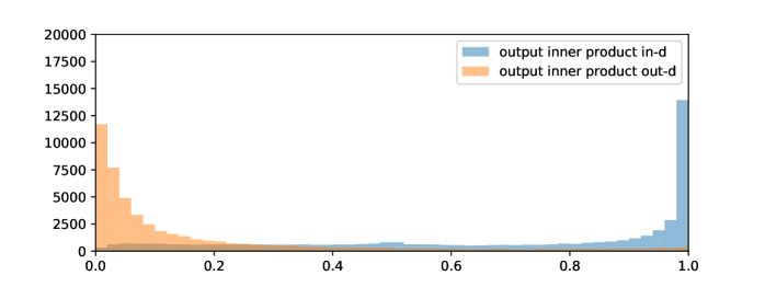
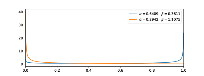
First, let us see the real in-distributions and out-distributions. Here we show two examples of ImageNet vs. Artificial dataset in Figure 10(a) and Figure 10(b). Then we run Beta fitting on the two examples and get Figure 10(c) and Figure 10(d). From the figures, we can see it is reasonable to model the in- and out- distributions as Beta distributions.


Next, let us focus on Lemma 5.3. Set and . We rewrite the expected runs as follows (we omit the small-o term):
We make a derivation on and get
where , and is defined as Digamma function, which is .
We make some discussions on the Digamma function .
Property 1. is increasing with respect to the variable .
According to its explict formula , and is the Euler–Mascheroni constant, we reach the above conclusion.
Property 2. .
Therefore, .
Therefore, when , we have ; when , we have .
Appendix E Transformation examples
Here we show several transformation examples from the ImageNet dataset in Figure 11.

Appendix F Detailed computational cost description of highly related algorithms
In Table 4, we briefly summarize the extra training and testing computational cost of highly related (standard classifier-based) algorithms. But we did not provide details because of space limitation. In this section, we will describe the details to clarify.
F.1 ODIN
After obtaining a standard classification model, ODIN requires input pre-processing, which first needs a forward pass to compute the loss, then a backpropagation to modify the input, and finally a forward pass again to calculate the final predicted probability values. The searching process of hyperparameters like noisy magnitude and temperature demands prior out-distribution knowledge.
F.2 Mahalanobis
Mahalanobis method assumes that the features of the in-distribution dataset follow a Gaussian distribution. It first needs forward all training samples to compute feature mean and variance. And then, it adopts a similar idea from input pre-processing, thus requires two forward passes and one backward pass to record the internal feature at test time. Meanwhile, the Mahalanobis method does a grid search across k (pre-determined) internal layers and several noise magnitude values. The best setting is selected with the help of prior out-distribution knowledge. After recording all the features of the test samples, it finally trains a regression model and gives final anomaly scores of test samples.
F.3 Ours
The computational cost of TTA-AD is almost the same as doubling testing a test point. We only need two forward passes per sample to compute the anomaly score. The pipeline is shown in Algorithm 1.
F.4 Running time of classifier based algorithms
For experiments in this section, we run all the running time experiments on an RTX 2080Ti graphic card. We only consider the CIFAR-10 vs. SVHN setting since the proportion of running time does not change with different datasets. For DenseNet-100, we conduct experiments similarly and the result is shown in Figure 12. And we omit the common classifier training time.
For ODIN, we slightly simplify the search space. According to the original ODIN paper, there are 210 times of searches in total. We only choose 44 among the 210 settings, which are useful in the CIFAR-10 vs. SVHN setting [25]. The Mahalanobis algorithm demands recording the mean and variance of the training samples, which takes about 19 seconds for the CIFAR-10 dataset in ResNet-34. This process will take more time if the training sample size increases. We follow the hyperparameter searching settings, which include 7 independent searches.
We do not mention other algorithms because they adopt other training ways which are significantly different from supervised training. For example, GAN-based algorithms require GAN training, which highly depends on the GAN algorithm. And obtaining a satisfying GAN usually takes a longer time than supervised classifier training. Contrastive learning aided algorithms [39] use contrastive methods (SimCLR [7]) to train a model, which takes much more time than standard classifier training. For example, SimCLR still gains performance improvement after 800 epochs training [7] and the computation of contrastive losses is more complicated. Considering the significant difference in pre-training time, we only compare the running time of our algorithm with these relatively lightweight standard classifier-based algorithms.
Appendix G Attempts for adapting previous algorithm
G.1 Network architecture
For CIFAR classifiers, we simply follow the common architectures which are also used by Liang et al. [25] and Lee et al. [24].
CIFAR models can not be directly used in ImageNet images. Following common configurations, we resize the ImageNet figures into 224x224, and use torchvision’s official ImageNet models: ResNet-50 and DenseNet-121 from https://pytorch.org/vision/stable/models.html. Standard normalization is added when pre-processing the images. For ImageNet subset training, we only change the output size of the last layer to the corresponding class numbers.
G.2 OC-SVM (One Class-SVM)
OC-SVM [35] is a general anomaly detection algorithm that trains a one-class SVM on a given (feature) dataset. The input of OC-SVM can be obtained from autoencoders, GANs, and plain classifiers. In our case, the classifier’s final output feature is used to train the OC-SVM. The only hyperparameter is bounded between 0 and 1, which acts as an upper bound on the fraction of margin errors and a lower bound of the fraction of support vectors relative to the total number of training examples. For both CIFAR and ImageNet settings, we linearly search the from 0.1 to 0.9 in intervals of 0.1.
The failure of OC-SVM on complex tasks is not surprising since it is usually used to perform anomaly detection at a more fine level, i.e., one-class-vs-all anomaly detection. For example, in the CIFAR-10 dataset, one of the classes is treated as in-distribution data while all other nine classes are considered as out-distribution data. But in our setting, multiple classes are treated as in-distribution data on the whole. One possible explanation for the failure is that we use larger models and harder classification tasks. So the features are more complicated than that of one-class-vs-all CIFAR, making the OC-SVM hard to find a good hyperplane.
G.3 MSP
G.4 ODIN
The major difference between ODIN [25] and the MSP method is that ODIN uses two techniques, input-preprocessing and temperature scaling, to enlarge the gap between the in-distribution and out-distribution samples in maximum predicted value. For both CIFAR and ImageNet subset settings, we do a grid search for noise value from [0, 0.0005, 0.001, 0.0014, 0.002, 0.0024, 0.005, 0.01, 0.05, 0.1, 0.2], and temperature value from [1, 10, 100, 1000].
G.5 Mahalanobis algorithm
For the CIFAR setting, we directly use the official setting mentioned in [24]. For the ImageNet subset settings, we use the official ResNet-50 and DenseNet-121 architecture from torchvision. The choice of internal output features is the same as the CIFAR setting: we choose the output of the first convolution layer and output of every transition layer for DenseNet, and the input of the first residual block and the output of every residual block for ResNet.
We also expand the hyperparameter search space. Specifically, we search the noise magnitude of the Mahalanobis method from [0.0, 0.5, 0.2, 0.1, 0.05, 0.02, 0.01, 0.005, 0.002, 0.0014, 0.001, 0.0005], which expands the original search space a lot. The validation dataset size is defined as 10% of the whole test set size, which is the same as the original paper.
Appendix H Classifier model training
Since we find the performance of classifier-based algorithms is highly based on the pre-trained classifier, e.g. different random seeds, we train three models for all settings and report the mean and variance. Standard training data augmentation methods are adopted, including resizing, padding and flipping. For full ImageNet training, we directly use pre-trained models from torchvision333https://pytorch.org/docs/stable/torchvision/models.html. The validation accuracy is for ResNet-50 and for DenseNet-121.
For ImageNet subset training, we use the official implementation of ResNet-50 and DenseNet-121 models from torchvision. We train 200 epochs using SGD with a stepping learning rate. The training and test accuracy is shown in Table 6.
| Subset | ResNet-50 | DenseNet-121 | ||
|---|---|---|---|---|
| Training | Test | Training | Test | |
| Living 9 | ||||
| Geirhos 16 | ||||
| Mixed 10 | ||||
For the CIFAR-10 dataset, we follow the training configuration from Lee et al. [24]. And the training and test result is shown in Table 7.
| Training acc. | Test acc. | |
|---|---|---|
| ResNet-34 | 100.000.00 | 94.840.12 |
| DenseNet-100 | 100.000.00 | 94.490.23 |
Appendix I Generalization of anomaly detection and CIFAR results
As mentioned by [50], when exposed to a new different out-distribution dataset, some previous algorithms suffer from severe performance degradation due to a severe bias introduced by validation bias. In the main text, TTA-AD has shown better average performance on advanced dataset settings like ImageNet. To verify whether our data augmentation and consistency evaluation pipeline has similar bias to anomaly detection datasets, we conduct CIFAR experiments to test whether there is a generalization problem of TTA-AD.
The performance on CIFAR-10 settings are shown in Table I. Specifically, the CIFAR-10 dataset is treated as in-distribution data, while the SVHN [28], TinyImageNet [22], and LSUN [48] datasets are out-distribution datasets. TTA-AD reaches the second best results with other algorithms on most settings. At the same time, we should notice that the best algorithm of CIFAR setting in Table I, i.e. the Mahalanobis, suffers from sever performance degradation in ImageNet settings Table 3, which is consistent with the observations from [50]. One possible reason is that the features of large network architectures and complicated datasets are not easy to be modeled as Gaussian distributions, which is the main assumption of the Mahalanobis algorithm. Another possible reason is that for ImageNet subset training, the test set size is not as large as CIFAR, so the hyperparameter searching process is difficult on ImageNet settings.
At the same time, our TTA-AD not only reaches higher average detection performance, but also shows stable generalization ability to low-resolution dataset settings.
| Architecture | Algorithm | Out-distribution data | ||
|---|---|---|---|---|
| SVHN | ImageNet_resize | LSUN_resize | ||
| ResNet-34 | MSP | |||
| OC-SVM | ||||
| ODIN | ||||
| Mahalanobis | ||||
| DenseNet-100 | MSP | |||
| OC-SVM | ||||
| ODIN | ||||
| Mahalanobis | ||||
Appendix J Sensitivity to filter radius
More sensitivity results for ImageNet subsets are in Figure 14 and Figure 14. In these figures, flatter curves mean less sensitivity to filter radius. For ImageNet subset settings, the optimal FFT filter radius seems to be much lower than that of the full ImageNet setting. A possible explanation is that the frequency domain characteristic of the Artificial dataset is different from the ImageNet dataset because artificial images are drawn by humans which lack fine-grained changes (high frequency signals). Meanwhile, we can see from Table 3 that no matter which radius is used, the performance is still good enough to outperform other algorithms.
Appendix K Sensitivity to temperature
See Figure 16 and Figure 16. Notice that for the ImageNet vs. Artificial setting, the dimension of the output is 1000. When the class number is big, temperature effect is enlarged a lot thus large temperature value leads to a relatively fast decreasing in the AUROC result(A brief explanation: Since the maximum output is much bigger than others, when calculating softmax, a large class number will lead to a big denominator value in the softmax equation). And for those whose output dimension is under 20, we can see that the AUROC results are not sensitive to temperature value.