Antifragility and response to damage in the synchronization of oscillators on networks

Let us consider a coupled system of oscillators on a connected, undirected network with $N$ nodes, indexed by $i=1,\ldots,N$. The phases $\theta_{i}(t)$ at each node evolve continuously over time $t$, starting at $t=0$. The network structure is characterized by a symmetric adjacency matrix $\mathbf{A}$, whose elements are defined as $A_{ij}=A_{ji}=1$ if there is a link connecting nodes $i$ and $j$, and $A_{ij}=A_{ji}=0$ otherwise. We use the notation $i\to j$ to represent a directed edge starting from node $i$ and ending at node $j$. The links are further described by an $N\times N$ matrix of weights $\mathbf{\Omega}$, with elements $\Omega_{ij}\geq 0$ for $i,j=1,\ldots,N$. The matrix $\mathbf{\Omega}$ is general in the sense that it incorporates both the network connectivity and specific weights for the links. Based on this information, we define the coupling matrix $\mathbf{W}(\mathbf{\Omega})$, with elements given by

$$w_{i\to j}(\mathbf{\Omega})\equiv\frac{\Omega_{ij}}{\mathcal{S}_{i}},$$

(1)

where $\mathcal{S}_{i}=\sum_{l=1}^{N}\Omega_{il}$ represents the generalized strength of node $i$ [44]. In this framework, the entries of the coupling matrix satisfy $0\leq w_{i\to j}(\mathbf{\Omega})\leq 1$ and are normalized such that $\sum_{l=1}^{N}w_{i\to l}(\mathbf{\Omega})=1$.
The evolution of the phases $\theta_{i}(t)$ of identical Kuramoto oscillators located at the nodes is governed by a system of coupled nonlinear differential equations

$$\frac{d\theta_{i}(t)}{dt}=\sum_{j=1}^{N}w_{i\to j}(\mathbf{\Omega})\sin[\theta_{j}(t)-\theta_{i}(t)]$$

(2)

for $i=1,2,\ldots,N$. This dynamics represents a generalization of the model introduced by Y. Kuramoto in Ref. [40] to the case of identical oscillators on weighted networks with a coupling matrix $\mathbf{W}(\mathbf{\Omega})$. For a detailed discussion of the Kuramoto model on networks, we refer the reader to Refs. [41, 43, 35].
Furthermore, one of the key features of the system described by Eq. (2) is that the phases can evolve to achieve a globally synchronized state. The conditions under which a system of identical Kuramoto oscillators reaches complete synchronization remain an active area of research. However, the topology of the network governing the coupling is known to play a crucial role [45, 46, 47, 48]. A commonly used quantity to measure the phase coherence of the oscillators is the macroscopic order parameter $r(t)$, defined as [41]

$$r(t)=\frac{1}{N}\left|\sum_{j=1}^{N}\exp\left[\mathbf{i}\,\theta_{j}(t)\right]\right|,$$

(3)

where $\mathbf{i}=\sqrt{-1}$. From the definition in Eq. (3), it follows that $0\leq r(t)\leq 1$. In the case of complete phase coherence, $r(t)=1$, whereas $r(t)=0$ corresponds to completely incoherent oscillators.
The evolution to a completely synchronized state in systems of identical Kuramoto oscillators implies that all oscillators eventually acquire identical phases. Strictly speaking, the time required for these systems to reach a fully synchronized state is infinite. However, this condition can be relaxed [18, 49]. For practical purposes, we analyze the time at which the systems are nearly synchronized, defined as the moment when the order parameter $r(t)$ reaches a predetermined fixed value $r$ close to 1. We refer to this specific time as the synchronization time. Equation (2) suggests that synchronization depends on the topology of the network, the coupling matrix $\mathbf{W}(\mathbf{\Omega})$, and the initial conditions of the system $\theta_{i}(0)$. When the initial phases are randomly chosen with a uniform distribution in the interval $[0,2\pi)$ for each node, synchronization times can be treated as a stochastic variable. A statistical analysis of this quantity provides valuable insights into the behavior of the system [18].

Previously, we introduced the Kuramoto model of identical oscillators on a weighted network. Let us now consider modifications to the matrix of weights $\mathbf{\Omega}$ and propose a measure to quantify the impact of these changes on global synchronization. Specifically, we examine how damage alters the matrix $\mathbf{\Omega}$, thereby affecting the coupling matrix $\mathbf{W}(\mathbf{\Omega})$ between the oscillators in the network and resulting in variations in synchronization times.
In the following, we assume that the function of the system with weights $\mathbf{\Omega}=\mathbf{A}$ and couplings described by $\mathbf{W}(\mathbf{A})$ is to achieve global synchronization starting from random initial phases. To evaluate the synchronization capacity of networks with modified weights, we define a second process incorporating a reorganization of the couplings in $\mathbf{W}(\mathbf{A})$, caused by a reduction in the capacity (damage) of the link $a\to b$ connecting nodes $a$ and $b$ in the network. This modification is represented by the matrix of weights $\mathbf{\Omega}^{\star}$, whose elements are defined as $\Omega^{\star}_{ab}=(1-\beta)A_{ab}$ for the damaged link, and $\Omega^{\star}_{ij}=A_{ij}$ otherwise. As a consequence of the definition in Eq. (1), the coupling matrices $\mathbf{W}(\mathbf{A})$ and $\mathbf{W}(\mathbf{\Omega}^{\star})$ with elements

$$w_{i\to j}(\mathbf{\Omega}^{\star})\equiv\frac{\Omega^{\star}_{ij}}{\sum_{l=1}^{N}\Omega^{\star}_{il}}=\cases{\displaystyle w_{i\to j}(\mathbf{A})\qquad\mathrm{if}\qquad i\neq a,\\ \displaystyle\frac{A_{aj}}{k_{a}-\beta}\hskip 34.1433pt\mathrm{if}\qquad i=a,\,\,j\neq b,\\ \displaystyle\frac{(1-\beta)A_{ab}}{k_{a}-\beta}\hskip 14.22636pt\mathrm{if}\qquad i=a,\,\,j=b,}$$

(4)

differ in the $a$-th row. The limit $\beta\to 0$ recovers the process used as reference defined by $\mathbf{W}(\mathbf{A})$. In this manner, the matrix of weights codifies the original capacity of the links, motivating the choice $\mathbf{\Omega}=\mathbf{A}$. However, in the modified matrix $\mathbf{\Omega}^{\star}$, the contribution of the specific link $a\to b$ to the system is reduced by a factor of $(1-\beta)$, representing damage to this particular link. Consequently, the normalization in the coupling matrix $\mathbf{W}(\mathbf{\Omega}^{\star})$ redistributes the shortages produced in link $a\to b$ equally among all links connected to node $a$. This type of normalized coupling is relevant in systems where, if a part of the structure fails (in this case, link $a\to b$), the remaining connections must compensate for the loss to maintain the global operation of the system.
On the other hand, let $\tau_{0}$ denote the synchronization time of the original (reference) network with couplings $\mathbf{W}(\mathbf{A})$, and let $\tau(\beta)$ represent the synchronization time when the weights have been altered due to damage, with couplings now described by $\mathbf{W}(\mathbf{\Omega}^{\star})$. In both cases, the initial phases at $t=0$ are chosen randomly with a uniform distribution in the interval $[0,2\pi)$ and maintained identical when evaluating $\tau_{0}$ and $\tau(\beta)$. Using this information, it is introduced the quantity [18]

$$\mathcal{F}_{\beta}\equiv\frac{\tau_{0}}{\tau(\beta)},$$

(5)

result obtained for one realization of the random initial conditions of the phases. In addition, we refer as “global functionality” to the ensemble average $\left\langle\mathcal{F}_{\beta}\right\rangle$ for several realizations of the values in Eq. (5). The average $\left\langle\mathcal{F}_{\beta}\right\rangle$ quantifies the global response of the system to a modification with value $\beta$ in the edge $a\to b$. In particular, we have $\left\langle\mathcal{F}_{\beta=0}\right\rangle=1$, and when considering the effect of an infinitesimal reduction in the capacity of the link, it is convenient to define

$$\Lambda^{(\mathrm{KM})}\equiv\frac{d\left\langle\mathcal{F}_{\beta}\right\rangle}{d\beta}\Bigg{|}_{\beta\to 0}.$$

(6)

The values $\Lambda^{(\mathrm{KM})}>0$ indicate cases where the reduction of the weight in the link $a\to b$ results in a global response that improves the system’s capacity to reach synchronization. This type of response is referred to as antifragile. Conversely, $\Lambda^{(\mathrm{KM})}<0$ is associated with fragility and reflects the reduction in synchronization capacity caused by the infinitesimal damage in the link $a\to b$. The result $\Lambda^{(\mathrm{KM})}=0$ is obtained in cases where the infinitesimal change in the weight of a specific link does not affect $\tau(\beta)$. In this regard, these interpretations depend on how the functionality in Eq. (5) is defined. In particular, this measure requires that both systems reach a fixed value $r$ close to 1 within a finite time. However, certain graph structures, such as cyclic graphs, rings, and circulant networks, do not satisfy this condition. In this sense, our measures in Eqs. (5) and (6) are only valid when the analyzed system achieves synchronization in both the original process defined by $\mathbf{\Omega}$, and the modified process given by $\mathbf{\Omega}^{\star}$.
Finally, it is important to highlight that the antifragility measured by Eq. (6) emerges from two combined effects: the reduction of the weight of the connection $a\to b$ and the redistribution of this weight among the links connected to node $a$, due to the normalization effect described in Eq. (4). However, the phenomenon of antifragility in synchronization processes can also be observed in systems where the couplings are not normalized (see Section 3.4 for an example illustrating this type of response to damage).

In the Kuramoto model, it has been shown that for initial conditions closer to synchronization, a linear approximation is valid [49, 50, 51]. In Eq. (2), for small values of $\theta_{j}(t)-\theta_{i}(t)$, the dynamics of the oscillators can be approximated linearly as

$$\frac{d\theta_{i}(t)}{dt}\approx\sum_{j=1}^{N}w_{i\to j}(\mathbf{\Omega})[\theta_{j}(t)-\theta_{i}(t)]=-\sum_{j=1}^{N}(\delta_{ij}-w_{i\to j}(\mathbf{\Omega}))\theta_{j}(t),$$

(7)

where $\delta_{ij}$ denotes the Kronecker delta. Thus, considering the form of the normalized Laplacian matrix of a weighted network [52, 53], we define the elements $\mathcal{L}_{ij}(\mathbf{\Omega})$ of the normalized Laplacian matrix $\hat{\mathcal{L}}(\mathbf{\Omega})$ as

$$\mathcal{L}_{ij}(\mathbf{\Omega})\equiv\delta_{ij}-w_{i\to j}(\mathbf{\Omega}).$$

(8)

Therefore, the linear approximation in Eq. (7) defines the dynamical process

$$\frac{d\theta_{i}(t)}{dt}=-\sum_{j=1}^{N}\mathcal{L}_{ij}(\mathbf{\Omega})\theta_{j}(t).$$

(9)

The integration of Eq. (9) leads to

$$\theta_{i}(t)=\sum_{j=1}^{N}\left(e^{-t\hat{\mathcal{L}}(\mathbf{\Omega})}\right)_{ij}\theta_{j}(0).$$

(10)

In addition, using Dirac’s notation for the eigenvectors, we have a set of right eigenvectors $\{\left|\phi_{j}(\mathbf{\Omega})\right\rangle\}_{j=1}^{N}$ that satisfy the eigenvalue equation $\hat{\mathcal{L}}(\mathbf{\Omega})\left|\phi_{j}(\mathbf{\Omega})\right\rangle=\xi_{j}(\mathbf{\Omega})\left|\phi_{j}(\mathbf{\Omega})\right\rangle$ for $j=1,\ldots,N$. The eigenvalues $\xi_{j}(\mathbf{\Omega})$ are ordered by their real part. For connected networks, we have $\xi_{1}(\mathbf{\Omega})=0$ and $0<\Re\{\xi_{2}(\mathbf{\Omega})\}\leq\Re\{\xi_{3}(\mathbf{\Omega})\}\leq\ldots\leq\Re\{\xi_{N}(\mathbf{\Omega})\}$, where $\Re\{\ldots\}$ denotes the real part of a complex number. Using the set of right eigenvectors, we define the matrix $\mathbf{Q}(\mathbf{\Omega})$ with elements $Q_{ij}(\mathbf{\Omega})\equiv\left\langle i|\phi_{j}(\mathbf{\Omega})\right\rangle$, and the diagonal matrix $\mathbf{\Upsilon}(t,\mathbf{\Omega})\equiv\textrm{diag}(e^{-t\xi_{1}(\mathbf{\Omega})},e^{-t\xi_{2}(\mathbf{\Omega})},\ldots,e^{-t\xi_{N}(\mathbf{\Omega})})$. These matrices satisfy

$$e^{-t\hat{\mathcal{L}}(\mathbf{\Omega})}=\mathbf{Q}(\mathbf{\Omega})\mathbf{\Upsilon}(t,\mathbf{\Omega})\mathbf{Q}(\mathbf{\Omega})^{-1},$$

(11)

where $\mathbf{Q}(\mathbf{\Omega})^{-1}$ is the inverse of $\mathbf{Q}(\mathbf{\Omega})$. Using the matrix $\mathbf{Q}(\mathbf{\Omega})^{-1}$, we define the set of left eigenvectors $\{\left\langle\bar{\phi}_{i}(\mathbf{\Omega})\right|\}_{i=1}^{N}$ with components $\left\langle\bar{\phi}_{i}(\mathbf{\Omega})|j\right\rangle=(\mathbf{Q}(\mathbf{\Omega})^{-1})_{ij}$. Therefore, the solution for the linear dynamics in Eq. (10) takes the form

$$\theta_{i}(t)=\sum_{j=1}^{N}\sum_{\ell=1}^{N}e^{-t\xi_{\ell}(\mathbf{\Omega})}\langle i|\phi_{\ell}(\mathbf{\Omega})\rangle\langle\bar{\phi}_{\ell}(\mathbf{\Omega})|j\rangle\theta_{j}(0).$$

(12)

Then, the effect of modifications in the matrix of weights $\mathbf{\Omega}$ in the linear approximation defines a process that can be explored analytically using the same methods developed in the study of the Kuramoto dynamics; however, all the temporal evolution is determined by the eigenvalues and eigenvectors of $\hat{\mathcal{L}}(\mathbf{\Omega})$. It is important to note that the linear dynamics is equivalent to the diffusive transport process associated with continuous-time random walks, defined by the normalized Laplacian with elements $\mathcal{L}_{ij}(\mathbf{\Omega})$ (although in our problem, the phase values are not restricted to be probabilities). This equivalence is our main motivation for incorporating the couplings $w_{i\to j}(\mathbf{\Omega})$ given by Eq. (1) into Eq. (2), which define the transition probabilities from node $i$ to $j$ of a random walker on a weighted network (see Ref. [44] for details).
The linear approximation in Eq. (9) and the analytical solution in Eq. (12) suggest two additional ways to define the global functionality of a system of coupled oscillators and the effect of infinitesimal modifications. For example, by solving numerically the set of linear equations in Eq. (9), we can calculate the synchronization times $\tau^{(\mathrm{linear})}_{0}$ for the reference process without damage and couplings $\mathbf{W}(\mathbf{A})$, and a time $\tau^{(\mathrm{linear})}(\beta)$ that characterizes the linear dynamics with couplings $\mathbf{W}(\mathbf{\Omega}^{\star})$, associated with modifications to the weights in the particular link $a\to b$. In this way, for a given synchronization threshold $r$, and using the same initial random conditions for both processes, we have

$$\mathcal{F}^{(\mathrm{linear})}_{\beta}\equiv\frac{\tau^{(\mathrm{linear})}_{0}}{\tau^{(\mathrm{linear})}(\beta)}.$$

(13)

Therefore, the average over several realizations gives the global functionality $\left\langle\mathcal{F}^{(\mathrm{linear})}_{\beta}\right\rangle$. Using this quantity, we define the effect of infinitesimal modifications in the link $a\to b$ as

$$\Lambda^{(\mathrm{linear})}\equiv\frac{d\left\langle\mathcal{F}^{(\mathrm{linear})}_{\beta}\right\rangle}{d\beta}\Bigg{|}_{\beta\to 0}.$$

(14)

The numerical evaluation of Eqs. (13) and (14) requires solving Eq. (9) or using all the eigenvalues and eigenvectors of $\hat{\mathcal{L}}(\mathbf{A})$ and $\hat{\mathcal{L}}(\mathbf{\Omega}^{\star})$. Both approaches lead to the same results but come with high computational costs. An alternative way to reduce the computational cost is to implement a different approach, commonly used in the study of synchronization, by considering the real part of the second eigenvalue $\xi_{2}(\mathbf{A})$ and $\xi_{2}(\mathbf{\Omega}^{\star})$ of the matrices $\hat{\mathcal{L}}(\mathbf{A})$ and $\hat{\mathcal{L}}(\mathbf{\Omega}^{\star})$ [54], respectively.
According to Eq. (12), $\tau^{(\xi_{2})}_{0}\equiv 1/\Re\{\xi_{2}(\mathbf{A})\}$ characterizes the synchronization time in the reference system, whereas $\tau^{(\xi_{2})}(\beta)=1/\Re\{\xi_{2}(\mathbf{\Omega^{\star}})\}$ describes the dynamics with modifications in the link $a\to b$. Therefore, it is reasonable to define a global functionality as

$$\mathcal{F}^{(\xi_{2})}_{\beta}\equiv\frac{\tau^{(\xi_{2})}_{0}}{\tau^{(\xi_{2})}(\beta)}=\frac{\Re\{\xi_{2}(\mathbf{\Omega^{\star}})\}}{\xi_{2}(\mathbf{A})},$$

(15)

where we use the fact that in undirected connected networks, $\xi_{2}(\mathbf{A})$ is a real number.
A particular feature of the global functionality $\mathcal{F}^{(\xi_{2})}_{\beta}$ is that it does not require averaging over initial conditions, making it easier to obtain than the values $\left\langle\mathcal{F}_{\beta}\right\rangle$ and $\left\langle\mathcal{F}^{(\mathrm{linear})}_{\beta}\right\rangle$. Finally, we can evaluate the effects of infinitesimal variations in the link $a\to b$ using

$$\Lambda^{(\xi_{2})}\equiv\frac{d\mathcal{F}^{(\xi_{2})}_{\beta}}{d\beta}\Big{|}_{\beta\to 0}.$$

(16)

In this section, we study a class of graphs known as lollipops, focusing on cases where the modification of a specific link induces an antifragile response at the global level. A lollipop graph of size $N$ is a network consisting of a fully connected subgraph (clique) with $N-L$ vertices and a linear path graph with $L$ nodes, connected by an additional edge referred to as the bridge. Our main motivation for studying lollipop graphs is that this structure combines a densely connected region with redundant couplings and a linear graph, which can be more fragile due to its lower connection density. In particular, in the context of diffusive transport on networks, cliques and communities exhibit an antifragile response [31]. With this idea in mind, in the following, we analyze the global functionality $\langle\mathcal{F}_{\beta}\rangle$ in Eq. (5) and $\Lambda^{(\mathrm{KM})}$ in Eq. (6) to explore the impact of damage in different lollipop graphs.
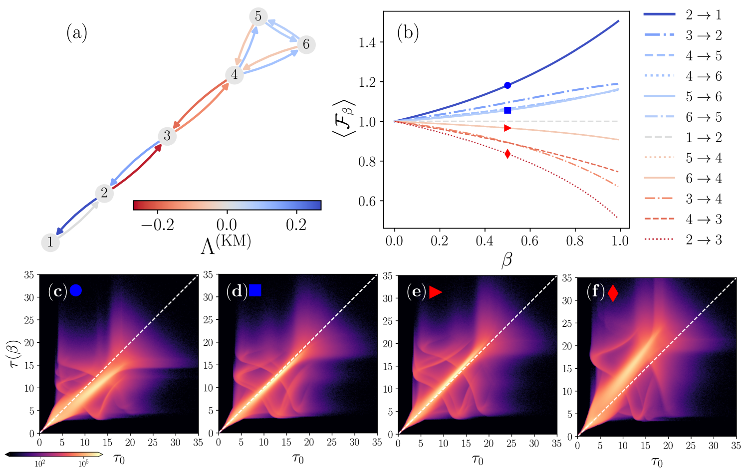
In Fig. 1, we analyze a lollipop graph with $N=6$ and $L=3$, as shown in Fig. 1(a). Figure 1(b) presents the ensemble average $\langle\mathcal{F}_{\beta}\rangle$ as a function of $\beta\in[0,1)$ for all directed edges in the graph. We use the notation $i\to j$ in the labels to indicate the direction of the edge, starting from node $i$ and ending at node $j$. The results were obtained using $10^{6}$ realizations to compute each value of $\langle\mathcal{F}_{\beta}\rangle$. Additionally, Fig. 1(a) includes the values of $\Lambda^{(\mathrm{KM})}$ for each edge, encoded in the colorbar in Fig. 1(a). These values were calculated with the derivative approximation in Eq. (6)

$$\Lambda^{(\mathrm{KM})}\approx\frac{1}{\Delta\beta}\left[\langle\mathcal{F}_{\Delta\beta}\rangle-1\right]$$

(17)

with $\Delta\beta=0.01$ and using $10^{7}$ realizations to evaluate $\langle\mathcal{F}_{\Delta\beta}\rangle$ in each edge. The curves in Fig. 1(b) are also colored according to the corresponding $\Lambda^{(\mathrm{KM})}$ values.
In Figs. 1(c)-(f), we present the statistical analysis of the synchronization times $\tau_{0}$ and $\tau(\beta)$ in four particular cases considering modifications with $\beta=0.5$ in different edges of the graph. Each histogram is obtained from the statistical analysis of synchronization using $10^{9}$ realizations of identical oscillators, with random initial phases uniformly distributed in the interval $[0,2\pi)$. For the calculation of each pair $(\tau_{0},\tau(\beta))$, the same initial conditions are maintained. The results show the effect of modifications in the links $2\to 1$ [Fig. 1(c)], $5\to 6$ [Fig. 1(d)], $6\to 4$ [Fig. 1(e)], and $2\to 3$ [Fig. 1(f)].
The results in Fig. 1 demonstrate the system’s antifragile or fragile global response to reductions in edge weights, depending on the specific edge modified. The values of $\Lambda^{(\mathrm{KM})}$ shown in Fig. 1(a), which correspond to infinitesimal edge modifications, allow the identification of antifragile links where $\Lambda^{(\mathrm{KM})}>0$. For these links, a reduction in the weight enhances the system’s synchronization capacity, resulting in $\langle\mathcal{F}_{\beta}\rangle>1$. This indicates that, for a significant fraction of initial conditions, $\tau(\beta)<\tau_{0}$. Similarly, for links with $\Lambda^{(\mathrm{KM})}<0$, a reduction in the weight is detrimental, leading to a global fragile response characterized by $\langle\mathcal{F}_{\beta}\rangle<1$. Additionally, in the case where $\Lambda^{(\mathrm{KM})}=0$ for the link $1\to 2$, changes with $\beta$ preserve the couplings $\mathbf{W}(\mathbf{\Omega}^{\star})$ due to the normalization imposed by Eq. (4). The different global responses of the oscillators, identified through infinitesimal variations in Eq. (17), remain valid for the interval $\beta\in(0,1)$, as shown in Fig. 1(b). For the analyzed lollipop graph, links with $\Lambda^{(\mathrm{KM})}>0$ exhibit a monotonic increase in $\langle\mathcal{F}_{\beta}\rangle$, whereas links with $\Lambda^{(\mathrm{KM})}<0$ show a monotonic decrease in functionality across the entire interval $0<\beta<1$.
Finally, it is important to emphasize that the values of $\langle\mathcal{F}_{\beta}\rangle$ provide only average information about the response to changes in synchronization times. Specifically, they reflect the differences between the average synchronization time $\tau_{0}$ of the oscillators in the original system and $\tau(\beta)$ in the modified system. In Figs. 1(c)-(f), we extend the analysis by constructing two-dimensional histograms of the pairs $(\tau_{0},\tau(\beta))$ for $\beta=0.5$, based on $10^{9}$ realizations of the initial conditions of the oscillator phases. The corresponding values of $\langle\mathcal{F}_{\beta}\rangle$ are highlighted with markers in Fig. 1(b), where two cases exhibiting an antifragile response and two cases with a fragile response are considered.
Figure 1(c) illustrates a case where the weight reduction occurs on the link $2\to 1$, which has the highest value of $\Lambda^{(\mathrm{KM})}$ and the largest increase in $\langle\mathcal{F}_{\beta}\rangle$. The results for this case indicate that, for a significant number of initial conditions, $\tau(\beta)<\tau_{0}$. This is evidenced by a greater density of points $(\tau_{0},\tau(\beta))$ below the dashed line representing $\tau(\beta)=\tau_{0}$. This imbalance leads to a value of $\langle\mathcal{F}_{\beta=0.5}\rangle=1.181$. A similar analysis is performed for a change with $\beta=0.5$ on the link $5\to 6$, which results in $\langle\mathcal{F}_{\beta=0.5}\rangle=1.056$ and also exhibits an antifragile response. In contrast, Figs. 1(e)-(f) depict cases with a fragile response, where a larger number of initial states produce responses with $\tau(\beta)>\tau_{0}$. In particular, the fragile response shown in Fig. 1(f), corresponding to modifications in the edge $2\to 3$, is the most pronounced. This case exhibits the smallest value of $\Lambda^{(\mathrm{KM})}$ and the largest reduction in $\langle\mathcal{F}_{\beta}\rangle$, with $\langle\mathcal{F}_{\beta=0.5}\rangle=0.836$.

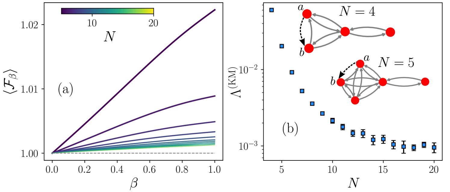
Our findings reported in Fig. 1 reveal the antifragile response observed in the link $5\to 6$ (or $6\to 5$), which is of particular interest. This type of link belongs to the clique, a structure where transportation processes involving random walks under damage conditions have demonstrated a strong antifragile response to weight reductions (see Ref. [31] for details). Motivated by this observation, in Fig. 2, we analyze the effects of modifications in lollipop graphs with $L=1$ and sizes varying from $N=4$ to $N=20$. We analyze the effect of reducing the weight of a link $a\to b$ in the clique that is not connected directly with the node that forms part of the bridge [this type of edge is illustrated in the link $a\to b$ in the graphs with $N=4,\,5$ presented as inset in Fig. 2(b)].
In Fig. 2(a), we present the numerical results for $\langle\mathcal{F}_{\beta}\rangle$ as a function of $\beta$ with $0\leq\beta<1$ for graphs with $L=1$ and sizes $5\leq N\leq 20$, as indicated by the colorbar. These values are obtained numerically using $10^{6}$ realizations for each $\beta\in[0,1)$, chosen with increments of $\Delta\beta=0.02$. In all cases, $\langle\mathcal{F}_{\beta}\rangle>1$ for $0<\beta<1$ (the limit $\langle\mathcal{F}_{\beta}\rangle=1$ is presented with a dashed line), indicating that the network’s capacity of synchronization increases with the effect of $\beta$ in the link $a\to b$. Additionally, the numerical results reveal that the reduction of the weight in this edge has a more pronounced impact on smaller structures.
On the other hand, the antifragility observed in Fig. 2(a) can be further analyzed by examining the derivative of $\langle\mathcal{F}_{\beta}\rangle$ evaluated at $\beta=0$. Specifically, the slope of the tangent line to $\langle\mathcal{F}_{\beta}\rangle$ at $\beta=0$ provides the value of $\Lambda^{(\mathrm{KM})}$, which indicates how a small, infinitesimal modification to the link $a\to b$ alters the global functionality. To quantify the numerical error of this measure, we analyze $10$ values of $\Lambda^{(\mathrm{KM})}$, each computed numerically using the approximation in Eq. (17) with $10^{7}$ realizations and $\Delta\beta=0.01$. In Fig. 2(b), we present $\Lambda^{(\mathrm{KM})}$ as a function of $N$ for lollipop graphs with $L=1$ and sizes $4\leq N\leq 20$. Square markers indicate the average values of $\Lambda^{(\mathrm{KM})}$, while the error bars represent the standard deviation of the computed values. The results show that the numerical variations in $\Lambda^{(\mathrm{KM})}$ lead to an error on the order of $10^{-4}$. The results in Fig. 2(b) illustrate how the antifragility of the analyzed link diminishes with increasing graph size $N$. Our findings indicate that in all cases studied, the response remains antifragile, with $\Lambda^{(\mathrm{KM})}>0$. However, the global impact of infinitesimal variations in the weights of this connection decreases significantly as the clique size grows, with a marked decline in graphs of size $N\leq 15$. For $N>15$, the reduction is less pronounced, but the uncertainties introduced by the numerical method become more noticeable, imposing limitations on the analysis of larger graphs with $N>20$.

The method described in Sections 3.1 and 3.2 for studying antifragility in lollipop graphs can be applied to analyze the impact of infinitesimal modifications on individual links in a graph. This approach allows the detection of edges whose reduction in their weight enhances, preserves, or diminishes the global capacity of the structure to reach synchronization. In this section, we study $\Lambda^{(\mathrm{KM})}$ for the edges of all connected non-isomorphic graphs with $N=6$ nodes. The analyzed graph set is available in Ref. [59] and includes 112 graphs with several topologies, such as diverse trees (e.g., linear and star graphs), networks with cycles and cliques of different sizes, and structures with high-density of links, including the fully connected graph. However, we focus exclusively on graphs that fully synchronize from random initial conditions. We exclude three specific cases: a ring with six nodes and two networks formed by a ring with five nodes plus one or two additional edges. Consequently, the final dataset analyzed consists of 109 graphs.

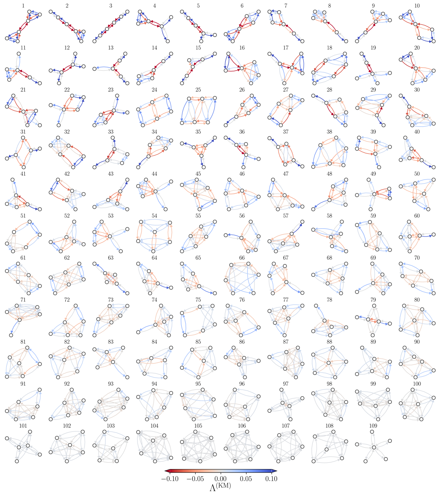
In Fig. 3, we present the numerical results obtained for $\Lambda^{(\mathrm{KM})}$, which evaluate the effect of infinitesimal modifications on each link in 109 non-isomorphic graphs. In this representation, each link is colored according to its respective $\Lambda^{(\mathrm{KM})}$, calculated numerically for each directed edge using Eq. (17) with $\Delta\beta=0.01$ and $10^{7}$ realizations to obtain the ensemble average, the values are codified in the colorbar. The graphs are sorted using the sum of the values $\Lambda^{(\mathrm{KM})}$ restricted to the antifragile links (those with with $\Lambda^{(\mathrm{KM})}>0$). Our findings show how antifragility emerge in the synchronization of oscillators and reveal that it is a challenge to identify a general rule for the distribution of links with $\Lambda^{(\mathrm{KM})}>0$ within the graph. However, in the first nine graphs, it is evident that structures connecting linear subgraphs with cliques or highly connected subgraphs exhibit links with greater antifragility. This pattern is observed in graph 1 (a barbell graph) formed by two cliques, the lollipop graphs 2 and 8, the trees 3 and 5, graph 4 (derived from the barbell graph by removing two directed links in one clique), and graph 6, which connects a clique with three nodes with a structure with four nodes. Graphs 7 and 9 similarly connect a subgraph with four nodes densely connected to a linear graph with two nodes.
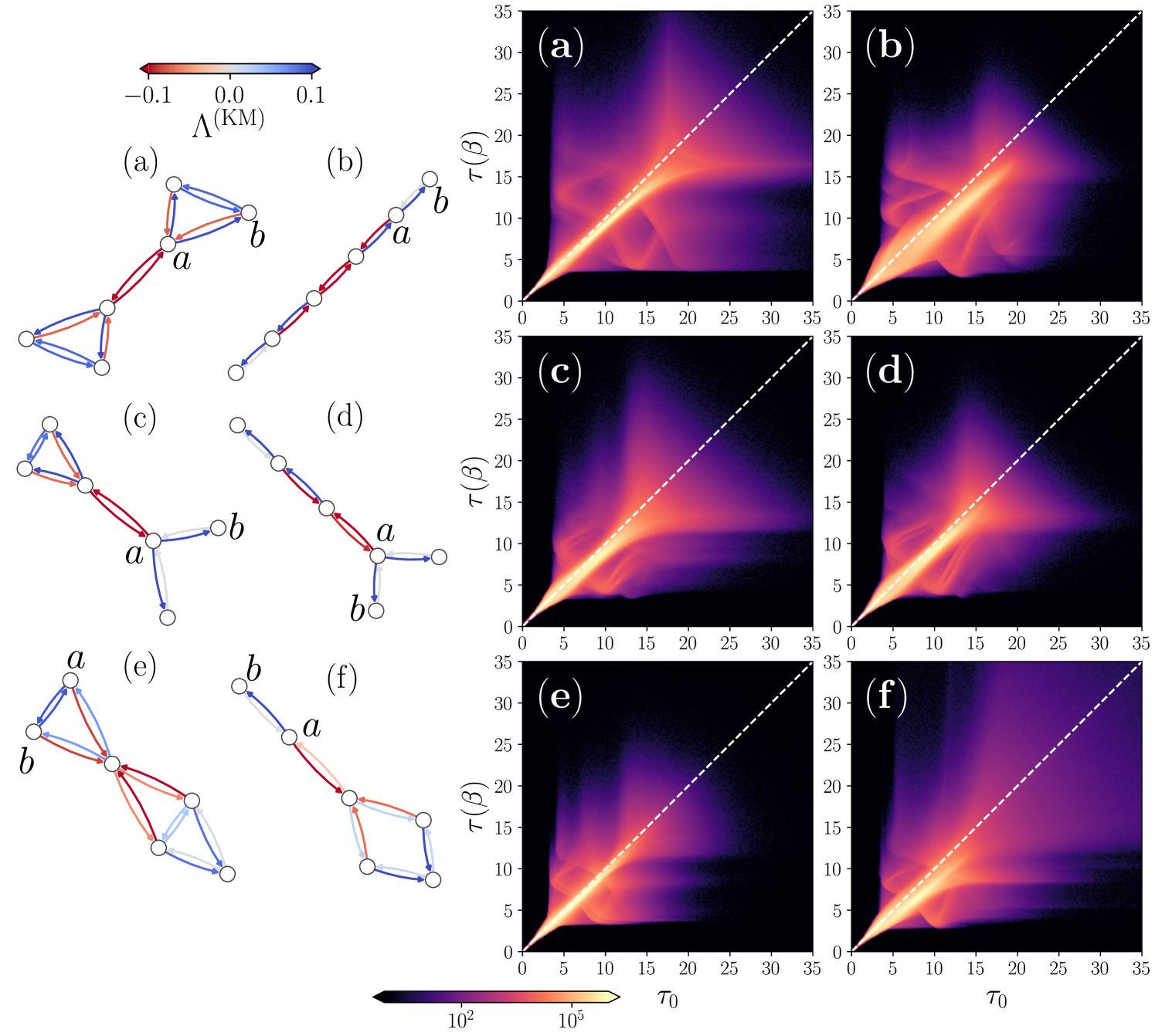
In Fig. 4, we complement the analysis of the antifragile response of the first graphs in Fig. 3 by exploring the synchronization times under modifications of the link $a\to b$ with the highest value of $\Lambda^{(\mathrm{KM})}$. For this link, we compute $10^{9}$ realizations of the synchronization times $\tau_{0}$ and $\tau(\beta)$ with $\beta=0.5$, using random initial phases. The analyzed graphs are shown in the left panels of Fig. 4, while the corresponding two-dimensional histograms of $(\tau_{0},\tau(\beta))$ are presented in the right panels. The numerical values are obtained by modifying the edge $a\to b$, with the respective nodes $a$ and $b$ highlighted in each graph. We examine graphs $1$ and $3$–$7$ from Fig. 3, while graph 2 was previously analyzed in detail in Fig. 1; in particular, Fig. 1(c) presents the results for the link with the highest antifragility. In Table 1, we report the ensemble average $\langle\tau_{0}\rangle$ of the times $\tau_{0}$ for the structure without damage, the highest value of $\Lambda^{(\mathrm{KM})}$ and the response to damage $\langle\mathcal{F}_{\beta=0.5}\rangle$ for the most antifragile link, each ensemble average is obtained using $10^{9}$ realizations.
Our findings in Fig. 4 and Table 1 indicate that for the analyzed links, a classification of $\Lambda^{(\mathrm{KM})}>0$ under infinitesimal weight variations consistently corresponds to an antifragile response, characterized by $\langle\mathcal{F}_{\beta}\rangle>1$ at $\beta=0.5$. Additionally, the two-dimensional histograms of $(\tau_{0},\tau(\beta))$ reveal a higher fraction of synchronization times from random initial phases satisfying $\tau(\beta)<\tau_{0}$, meaning that more values fall below the dashed line $\tau_{0}=\tau(\beta)$.

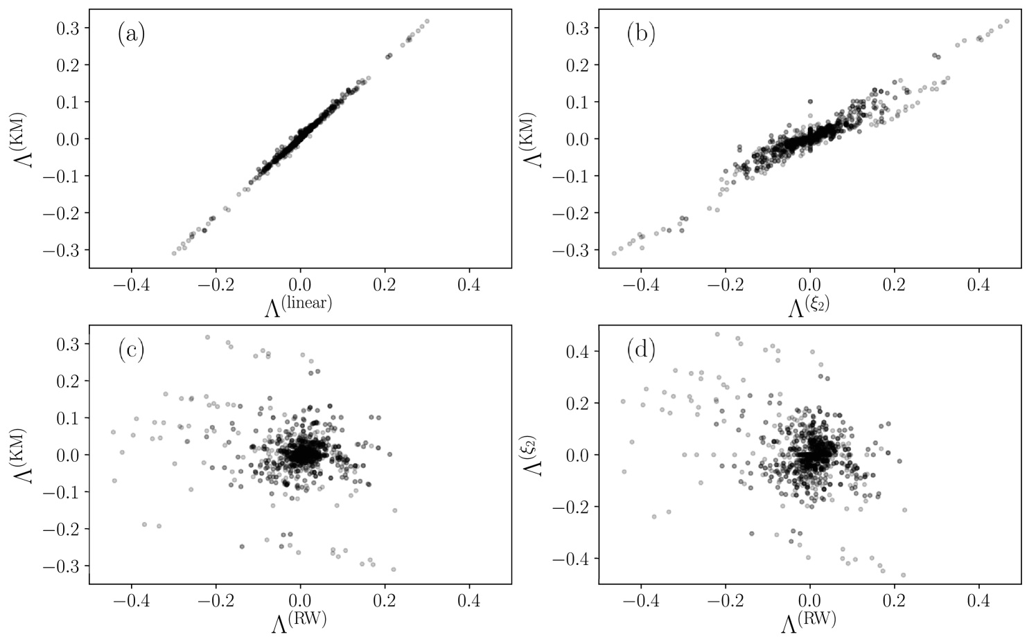
After calculating $\Lambda^{(\mathrm{KM})}$ for all the edges in the graphs analyzed in Fig. 3, we use this information to investigate the relationship between $\Lambda^{(\mathrm{KM})}$ and other quantities introduced in Section 2 for evaluating dynamical systems associated with the Kuramoto model. To this end, in Fig. 5, we present scatter plots of points with coordinates $(\Lambda_{x},\Lambda_{y})$, where $\Lambda_{x}$ and $\Lambda_{y}$ represent two measures of the response to modifications of the same edge in the graph. The quantities analyzed include $\Lambda^{(\mathrm{KM})}$ defined in Eq. (17), $\Lambda^{(\mathrm{linear})}$ in Eq. (14), $\Lambda^{(\xi_{2})}$ in Eq. (16), and $\Lambda^{(\mathrm{RW})}$ in Eq. (19), which characterizes the effect of damage in transportation processes associated with random walks on networks [31], see Appendix 5 for details.
In Fig. 5(a), we compare $\Lambda^{(\mathrm{KM})}$ with $\Lambda^{(\mathrm{linear})}$. Specifically, calculating $\Lambda^{(\mathrm{linear})}$ involves numerically solving the linear system of equations in Eq. (9) to determine the synchronization times $\tau^{(\mathrm{linear})}_{0}$ and $\tau^{(\mathrm{linear})}(\beta)$ starting from random initial phases. By using these values is computed numerically

$$\Lambda^{(\mathrm{linear})}=\frac{1}{\Delta\beta}\left[\left\langle\mathcal{F}_{\beta}^{(\mathrm{linear})}\right\rangle-1\right].$$

(18)

The results are obtained with $\Delta\beta=0.01$ and $10^{7}$ realizations. Our findings in Fig. 5(a) reveal a linear relationship between $\Lambda^{(\mathrm{KM})}$ and $\Lambda^{(\mathrm{linear})}$, with subtle deviations from this trend. These deviations indicate that, in most cases, the Kuramoto model and its linear approximation yield similar classifications of edges as antifragile, neutral, or fragile in the analyzed graphs. However, an important consideration when evaluating $\Lambda^{(\mathrm{KM})}$ and $\Lambda^{(\mathrm{linear})}$ is that both have the same computational cost, as they require solving differential equations numerically and averaging over initial conditions. Given this, it is more practical to compute $\Lambda^{(\mathrm{KM})}$ to assess the response of links in the network.
In contrast, Fig. 5(b) presents the relationship between $\Lambda^{(\mathrm{KM})}$ and $\Lambda^{(\xi_{2})}$. Calculating $\Lambda^{(\xi_{2})}$ is computationally faster than $\Lambda^{(\mathrm{KM})}$, as evaluating Eq. (16) requires only the second smallest eigenvalue of the matrices $\hat{\mathcal{L}}(\mathbf{A})$ and $\hat{\mathcal{L}}(\mathbf{\Omega}^{\star})$. The scatter plot of points in Fig. 5(b) reveals a linear relationship between $\Lambda^{(\mathrm{KM})}$ and $\Lambda^{(\xi_{2})}$, with notable deviations. In particular, for $|\Lambda^{(\mathrm{KM})}|<0.1$, several cases exhibit discrepancies in the signs of $\Lambda^{(\mathrm{KM})}$ and $\Lambda^{(\xi_{2})}$, leading to different classifications of edge responses to modifications. However, for $|\Lambda^{(\mathrm{KM})}|\geq 0.1$, the classifications of fragility or antifragility are consistent between both measures. These findings suggest that $\Lambda^{(\xi_{2})}$ can serve as a fast method to identify edges with significant fragile or antifragile responses to weight modifications.
Furthermore, the relationship between the linear dynamics in Eq. (9), defined by the modified Laplacian $\hat{\mathcal{L}}(\mathbf{\Omega})$, and the transition matrix of a random walker on a weighted network, $\mathbf{W}(\mathbf{\Omega})$, motivates the exploration of how our findings relate to antifragility when the network’s primary function is to reach efficiently all the nodes through the movement of a random walker. In Fig. 5(c), we present the pairs $(\Lambda^{(\mathrm{RW})},\Lambda^{(\mathrm{KM})})$, where $\Lambda^{(\mathrm{RW})}$ is calculated using the numerical approximation of Eq. (25) in Appendix 5

$$\Lambda^{(\mathrm{RW})}\approx\frac{1}{\Delta\beta}\left[\mathcal{F}^{(\mathrm{RW})}_{\Delta\beta}-1\right]$$

(19)

with $\Delta\beta=10^{-4}$. In this case, the distribution of points in Fig. 5(c) shows no discernible relationship between $\Lambda^{(\mathrm{RW})}$ and $\Lambda^{(\mathrm{KM})}$. Consequently, there is no direct connection between the antifragile or fragile response measured by these quantities, highlighting that the classification of edges based on their response to damage depends on the graph, the perturbed link, and the specific dynamical process occurring on the structure. As an additional test to the measures explored, Fig. 5(d) presents an analysis of the quantities $\Lambda^{(\xi_{2})}$ and $\Lambda^{(\mathrm{RW})}$. Once again, no correlation is observed between these two measurements, indicating no relationship between the antifragility measured in diffusive transport processes on networks and the dynamics whose global function is the synchronization of coupled oscillators.

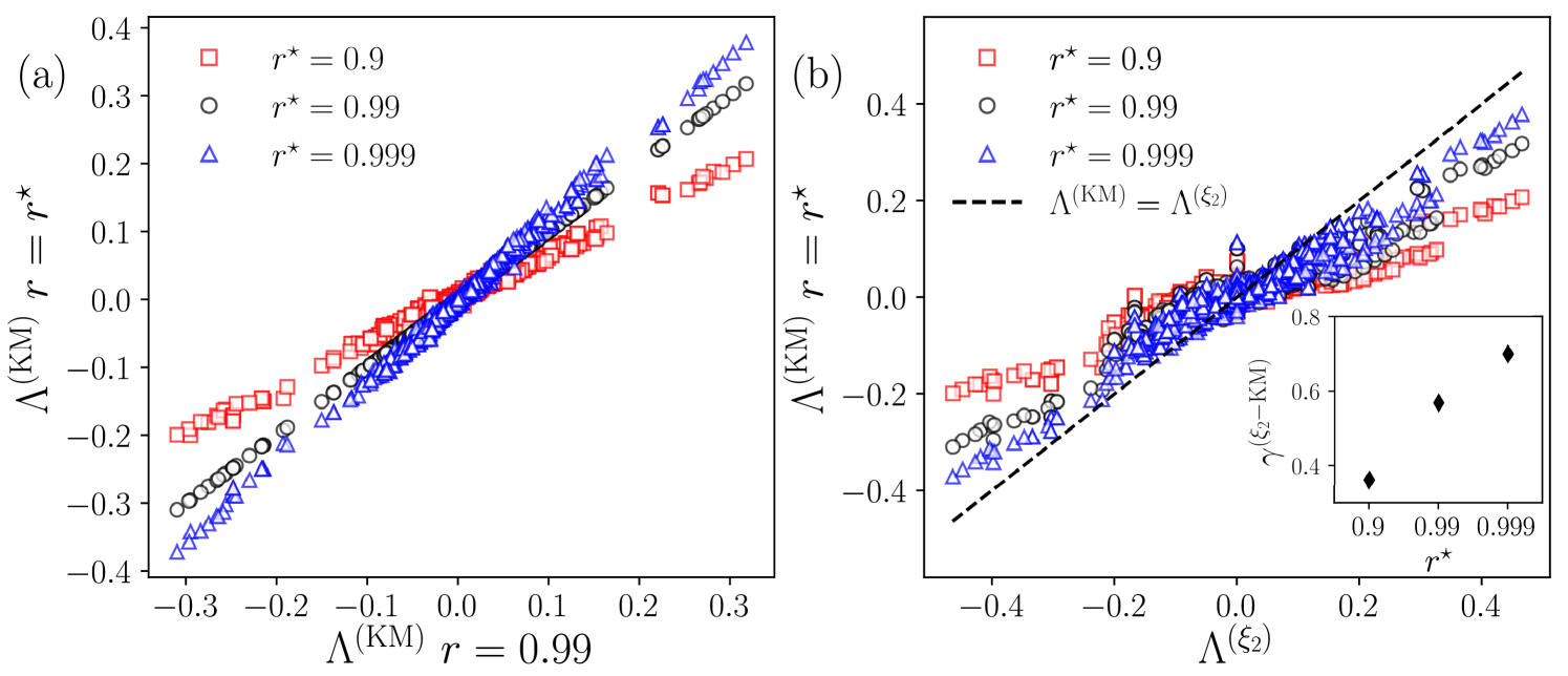
Once $\Lambda^{(\mathrm{KM})}$ and its relationship with other related quantities have been explored in Fig. 5, it is important to note that all the results presented for $\Lambda^{(\mathrm{KM})}$ in Figs. 3–5 rely on the functionality $\mathcal{F}_{\beta}$ defined in Eq. (5), where the synchronization times are computed using the threshold $r=0.99$ for the order parameter in Eq. (3). However, it is crucial to understand how the classification of antifragility and fragility provided by $\Lambda^{(\mathrm{KM})}$ for all edges in the graphs of Fig. 3 is affected by the choice of different values of the threshold $r$. To this end, in Fig. 6 we analyze the values of $\Lambda^{(\mathrm{KM})}$ obtained using three different thresholds for the order parameter: $r=0.9$, $0.99$, and $0.999$, considering all edges of the graphs with $N=6$ explored in Fig. 3 with $10^{7}$ realizations to obtain $\Lambda^{(\mathrm{KM})}$.
In Fig. 6(a), we present the pairs $(\Lambda_{x},\Lambda_{y})$, where $\Lambda_{x}$ corresponds to the values computed using the threshold $r=0.99$, these values were previously shown in Fig. 3 and analyzed in Fig. 5. The corresponding $\Lambda_{y}$ denotes $\Lambda^{(\mathrm{KM})}$ obtained for the same links but using the thresholds $r=r^{\star}$, with $r^{\star}=0.9$, $0.99$, and $0.999$. The resulting scatter plot is shown using different markers for each value of $r^{\star}$. The numerical results reported in Fig. 6(a) reveal a strong linear relationship between the values of $\Lambda^{(\mathrm{KM})}$ computed with $r=0.99$ and those obtained using the thresholds $r=0.9$ and $r=0.999$. Additionally, it is evident that $|\Lambda^{(\mathrm{KM})}|$ tends to increase as $r$ approaches 1. In particular, for links with $\Lambda^{(\mathrm{KM})}>0$, the antifragility increases for higher values of $r$. It is also worth noting that the antifragility/fragility classifications derived from $\Lambda^{(\mathrm{KM})}$ for the $r$ explored remain similar to those presented in Fig. 3.
In Fig. 6(b), we complement the analysis by exploring the relationship between the values of $\Lambda^{(\mathrm{KM})}$ obtained for $r=r^{\star}=0.9$, $0.99$, and $0.999$, and the corresponding values of $\Lambda^{(\xi_{2})}$ calculated using Eq. (16). The latter has the advantage of not requiring ensemble averages or the specification of a particular threshold, providing a more direct method to characterize the system’s response to damage. The results obtained from the scatter plot of points $(\Lambda^{(\xi_{2})},\Lambda^{(\mathrm{KM})})$ reveal linear trends. However, noticeable deviations suggest that the approximation given by $\Lambda^{(\xi_{2})}$ does not fully capture the impact of damage as quantified by $\Lambda^{(\mathrm{KM})}$. Furthermore, by performing a linear fit of the form $\Lambda^{(\mathrm{KM})}=\gamma^{(\xi_{2}-\mathrm{KM})}\Lambda^{(\xi_{2})}+\mathcal{C}$, we find that $\mathcal{C}\approx 0.003$, a value that is effectively within the numerical error margin of $\Lambda^{(\mathrm{KM})}$. The corresponding slopes $\gamma^{(\xi_{2}-\mathrm{KM})}$ for each case are reported in the inset of Fig. 6(b). It is observed that $\gamma^{(\xi_{2}-\mathrm{KM})}$ increases with $r$, approaching the limiting case in which $\Lambda^{(\mathrm{KM})}=\Lambda^{(\xi_{2})}$. In general, the analysis presented in Fig. 6(b) provides additional evidence of antifragility in graphs and shows that this effect can also be captured through $\Lambda^{(\xi_{2})}$, which is computationally more accessible. This alternative measure enables the identification of links with a strong response to damage, particularly when $|\Lambda^{(\mathrm{KM})}|\geq 0.2$. For lower values, i.e., when $|\Lambda^{(\mathrm{KM})}|<0.2$, nonlinear effects may be important in the evaluation of the consequences of damage. These effects are captured by $\Lambda^{(\mathrm{KM})}$ but not by $\Lambda^{(\xi_{2})}$.

In the Kuramoto model defined by Eq. (2), the interactions are given by the elements of $\mathbf{W}(\mathbf{\Omega})$. These couplings include a normalization that causes the effect of the damage represented by $\mathbf{W}(\mathbf{\Omega}^{\star})$, with elements given by Eq. (4), to incorporate two combined effects: the reduction of the weight on a specific link and the redistribution of the lost function by other connections in the network. In order to explore the existence of antifragility in coupled oscillators emerging solely from the reduction of the coupling weight $\mathbf{\Omega}$, this section analyzes synchronization processes defined by a Kuramoto model with non-normalized coupling weights.
We start with the Kuramoto model for identical oscillators with non-normalized couplings [18]

$$\frac{d\theta_{i}(t)}{dt}=\sum_{j=1}^{N}\Omega_{ij}\sin[\theta_{j}(t)-\theta_{i}(t)],$$

(20)

choosing the weights $\mathbf{\Omega}=\mathbf{A}$ in a system that reaches synchronization up to a given threshold value $r$, for which the time $\tau_{0}$ is defined.
Similarly, synchronization is studied in a modified system with weights $\mathbf{\Omega}^{\star}$, where damage is introduced in the link $a\to b$: $\Omega^{\star}_{ab}=(1-\beta)A_{ab}$ (the rest of the entries coincide with the original weights in $\mathbf{\Omega}$). This new system evolves according to the following set of differential equations

$$\frac{d\theta_{i}(t)}{dt}=\sum_{j=1}^{N}\Omega^{\star}_{ij}\sin[\theta_{j}(t)-\theta_{i}(t)].$$

(21)

In this case, $\tau(\beta)$ denotes the time required to reach the order parameter $r$. From the information given by $\tau_{0}$ and $\tau(\beta)$, obtained under the same random initial condition for the phases (chosen from a uniform distribution), we compute the functionality $\mathcal{F}_{\beta}=\frac{\tau_{0}}{\tau(\beta)}$ and the coefficient $\Lambda^{(\mathrm{KM-NNC})}$, which measures the response to damage for infinitesimal variations in the link $a\to b$ and is calculated numerically as

$$\Lambda^{(\mathrm{KM-NNC})}\approx\frac{1}{\Delta\beta}\left[\langle\mathcal{F}_{\Delta\beta}\rangle-1\right]$$

(22)

for a small value $\Delta\beta$.
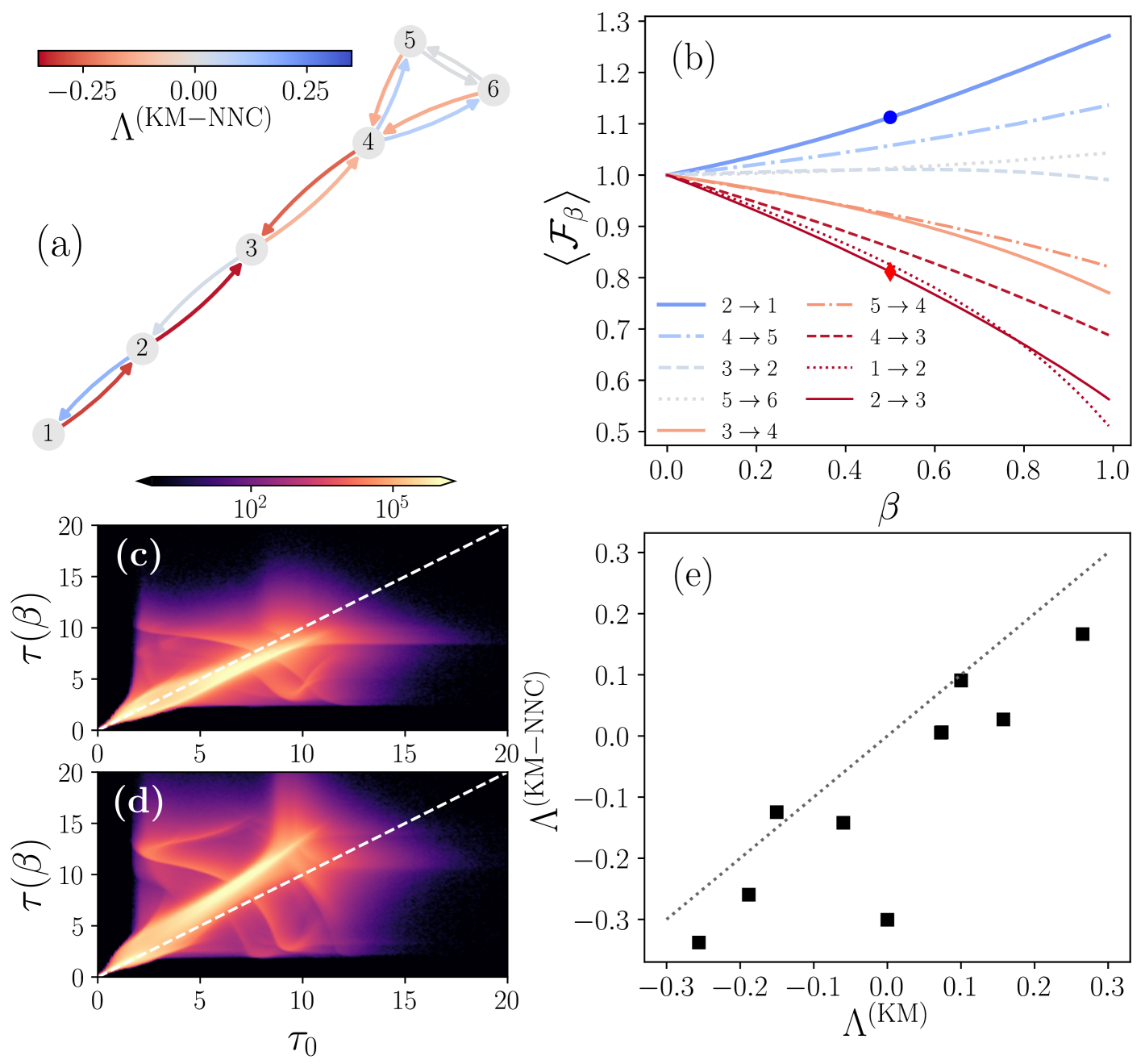
In order to illustrate the effect of damage in synchronization processes where the couplings are not normalized, in Fig. 7 we show different results for the study of the lollipop graph previously analyzed in Fig. 1. All the numerical values are obtained using the synchronization threshold $r=0.99$.
Figure 7(a) depicts the analyzed graph. The value $\Lambda^{(\mathrm{KM-NNC})}$ is obtained for each edge using Eq. (22) with $\Delta\beta=0.01$ and $10^{7}$ realizations to compute the ensemble averages (the results are encoded in the colorbar). Figure 7(b) shows the ensemble average $\langle\mathcal{F}_{\beta}\rangle$ as a function of $\beta\in[0,1)$ for all directed edges in the graph (the cases $4\to 6$, $6\to 4$, and $6\to 5$ are not included due to their symmetry with other edges). We use $10^{6}$ realizations to compute each value of $\langle\mathcal{F}_{\beta}\rangle$. The curves were ordered according to the corresponding values of $\Lambda^{(\mathrm{KM-NNC})}$, from the largest to the smallest. On the other hand, Figs. 7(c)-(d) show the statistical analysis of the pairs $(\tau_{0},\tau(\beta))$, with $\beta=0.5$ and $10^{9}$ realizations, for the edges $2\to 1$ [in Fig. 7(c)], which exhibits the largest antifragile response, and $2\to 3$ [in Fig. 7(d)], which corresponds to the most fragile response. The respective functionality of these cases, for $\beta=0.5$, is indicated with a marker in Fig. 7(b).
For the antifragile response shown in Fig. 7(c), a higher density of points is observed below the dashed line, corresponding to scenarios where $\tau_{0}>\tau(\beta)$. In contrast, in Fig. 7(d), the response of the system is fragile, with a more significant number of random initial conditions producing $\tau_{0}<\tau(\beta)$. Additionally, it is worth highlighting that the patterns observed in Figs. 7(c)-(d) are similar to those found in Figs. 1(c)-(f), showing regions with a higher density of time pairs $(\tau_{0},\tau(\beta))$ associated with specific responses of the system under different initial conditions.
Figure 7(e) compares the results obtained for $\Lambda^{(\mathrm{KM-NNC})}$ from Eq. (22) with those obtained for $\Lambda^{(\mathrm{KM})}$ from Eq. (17), using the values corresponding to all the links of the graph analyzed in Fig. 7(a). The results reveal that, when the dynamics are governed by non-normalized couplings, a new classification of the links emerges based on their response to damage. Moreover, it is important to highlight that, in most cases, the inequality $\Lambda^{(\mathrm{KM-NNC})}<\Lambda^{(\mathrm{KM})}$ holds, as shown by the points located below the dashed line representing $\Lambda^{(\mathrm{KM-NNC})}=\Lambda^{(\mathrm{KM})}$. The only exception to this behavior corresponds to the link $3\to 4$, where the application of infinitesimal damage results in $\Lambda^{(\mathrm{KM-NNC})}>\Lambda^{(\mathrm{KM})}$.
The results presented in Fig. 7 provide evidence of a case where the effect of antifragility emerges when the coupling weights are not normalized. This observation suggests that antifragility is an inherent property of synchronization processes, which can be further enhanced in systems where, after damage to a specific link, other parts of the system compensate by absorbing the lost functionality. Finally, the findings presented in this section demonstrate the general applicability of the proposed methods for characterizing antifragility and fragility in systems of coupled oscillators that reach synchronization, i.e., in cases where it is possible to compute the times $\tau_{0}$ and $\tau(\beta)$, which remain finite for a given synchronization threshold $r$.

References

- [1] Bar-yam Y 1997 Dynamics of Complex Systems (Boston: Addison-Wesley)
- [2] Sayama H 2015 Introduction to the Modeling and Analysis of Complex Systems (Geneseo, New York: Open SUNY Textbooks)
- [3] Barrat A, Barthélemy M and Vespignani A 2008 Dynamical Processes on Complex Networks (Cambridge: Cambridge University Press)
- [4] Carlson J M and Doyle J 2000 Phys. Rev. Lett. 84 2529–2532
- [5] Carlson J M and Doyle J 2002 Proc. Natl. Acad. Sci. U.S.A 99 2538–2545
- [6] Dobson I, Carreras B A, Lynch V E and Newman D E 2007 Chaos 17 026103
- [7] Sun E D, Michaels T C T and Mahadevan L 2020 Proc. Natl. Acad. Sci. USA 117 20404–20410
- [8] Vural D C, Morrison G and Mahadevan L 2014 Phys. Rev. E 89 022811
- [9] Cohen A A 2016 Biogerontology 17 205–20
- [10] Barabási A L 2016 Network science (Cambridge: Cambridge University Press) ISBN 9781107076266 1107076269
- [11] Katifori E, Szöllősi G J and Magnasco M O 2010 Phys. Rev. Lett. 104 048704
- [12] Farr R S, Harer J L and Fink T M A 2014 Phys. Rev. Lett. 113 138701
- [13] Hu F, Yeung C H, Yang S, Wang W and Zeng A 2016 Sci. Rep. 6 24522
- [14] Lin Z H, Feng M, Tang M, Liu Z, Xu C, Hui P M and Lai Y C 2020 Nat. Commun. 11 2490
- [15] Riascos A P, Wang-Michelitsch J and Michelitsch T M 2019 Phys. Rev. E 100 022312
- [16] Eraso-Hernandez L K, Riascos A P, Michelitsch T M and Wang-Michelitsch J 2021 J. Stat. Mech. 2021 063401
- [17] Eraso-Hernandez L K, Riascos A P, Michelitsch T M and Wang-Michelitsch J 2023 Int. J. Mod. Phys. C 2450037
- [18] Eraso-Hernandez L K and Riascos A P 2023 J. Phys. A: Math. Theor. 56 475001
- [19] Faci-Lázaro S, Lor T, Ródenas G, Mazo J J, Soriano J and Gómez-Gardeñes J 2022 Eur. Phys. J.: Spec. Top. 231 195–201
- [20] Teller S, Estévez-Priego E, Granell C, Tornero D, Andilla J, Olarte O E, Loza-Alvarez P, Arenas A and Soriano J 2020 eNeuro 7 ENEURO.0254
- [21] Ayasreh S, Jurado I, López-León C F, Montalà-Flaquer M and Soriano J 2022 Micromachines 13 2259
- [22] Taleb N N 2012 Antifragile (New York: Random House)
- [23] Alatorre D, Gershenson C and Mateos J L 2023 PLOS ONE 18 e0280487
- [24] Coppitters D and Contino F 2023 Sci. Rep. 13 9138
- [25] Equihua M, Espinosa Aldama M, Gershenson C, López-Corona O, Munguía M, Pérez-Maqueo O and Ramírez-Carrillo E 2020 PeerJ 8 e8533
- [26] Axenie C, López-Corona O, Makridis M A, Akbarzadeh M, Saveriano M, Stancu A and West J 2024 npj Complexity 1 12
- [27] Youn H, Gastner M T and Jeong H 2008 Phys. Rev. Lett. 101(12) 128701
- [28] Pineda O K, Kim H and Gershenson C 2019 Complexity 2019 3728621
- [29] López-Díaz A J, Sánchez-Puig F and Gershenson C 2023 Entropy 25 254
- [30] Ghodrat M, Naji A, Komaie-Moghaddam H and Podgornik R 2015 Soft Matter 11(17) 3441–3459
- [31] Eraso-Hernandez L K and Riascos A P 2024 Phys. Rev. E 110 044309
- [32] Boccaletti S 2008 The synchronized dynamics of complex systems The Synchronized Dynamics of Complex Systems (Monograph Series on Nonlinear Science and Complexity vol 6) ed Boccaletti S (Elsevier) pp 1–239
- [33] Pikovsky A, Rosenblum M and Kurths J 2003 Synchronization A Universal Concept in Nonlinear Sciences (Cambridge: Cambridge University Press)
- [34] Strogatz S H 2003 Sync: The Emerging Science of Spontaneous Order (New York: Hyperion)
- [35] Ji P, Ye J, Mu Y, Lin W, Tian Y, Hens C, Perc M, Tang Y, Sun J and Kurths J 2023 Phys. Rep. 1017 1–96
- [36] Sarfati R, Hayes J C and Peleg O 2021 Sci. Adv. 7 eabg9259
- [37] Néda Z, Ravasz E, Vicsek T, Brechet Y and Barabási A L 2000 Phys. Rev. E 61(6) 6987–6992
- [38] Wiesenfeld K, Colet P and Strogatz S H 1996 Phys. Rev. Lett. 76(3) 404–407
- [39] Balanov A, Janson N, Postnov D and Sosnovtseva O 2009 Synchronization: From Simple to Complex (Berlin, Heidelberg: Springer Berlin Heidelberg)
- [40] Kuramoto Y 1984 Chemical Oscillations, Waves, and Turbulence (Berlin, Heidelberg: Springer Berlin, Heidelberg)
- [41] Arenas A, Díaz-Guilera A, Kurths J, Moreno Y and Zhou C 2008 Phys. Rep. 469 93 – 153
- [42] Tang Y, Qian F, Gao H and Kurths J 2014 Annu. Rev. Control 38 184–198
- [43] Rodrigues F A, Peron T K, Ji P and Kurths J 2016 Phys. Rep. 610 1–98
- [44] Riascos A P and Mateos J L 2021 J. Complex Netw. 9 cnab032
- [45] Taylor R 2012 J. Phys. A: Math. Theor. 45 055102
- [46] Townsend A, Stillman M and Strogatz S H 2020 Chaos 30 083142
- [47] Ling S, Xu R and Bandeira A S 2019 SIAM J. Optim. 29 1879–1907
- [48] Ha S Y, Ha T and Kim J H 2010 Phys. D: Nonlinear Phenom. 239 1692–1700
- [49] Almendral J A and Díaz-Guilera A 2007 New J. Phys. 9 187
- [50] Grabow C, Hill S M, Grosskinsky S and Timme M 2010 EPL (Europhysics Letters) 90 48002
- [51] Grabow C, Grosskinsky S and Timme M 2011 Eur. Phys. J. B 84 613–626
- [52] Michelitsch T M, Riascos A P, Collet B A, Nowakowski A F and Nicolleau F C G A 2019 Fractional Dynamics on Networks and Lattices (London: ISTE/Wiley)
- [53] Riascos A P and Padilla F H 2023 J. Phys. A Math. Theor. 56 145001
- [54] Aguirre J, Sevilla-Escoboza R, Gutiérrez R, Papo D and Buldú J M 2014 Phys. Rev. Lett. 112 248701
- [55] Muller L, Mináč J and Nguyen T T 2021 Phys. Rev. E 104 L022201
- [56] Ódor G and Kelling J 2019 Sci. Rep. 9 19621
- [57] Böhle T, Kuehn C and Thalhammer M 2022 Int. J. Comput. Math. 99 31–57
- [58] Lam S K, Pitrou A and Seibert S 2015 Numba: A llvm-based python jit compiler Proceedings of the Second Workshop on the LLVM Compiler Infrastructure in HPC pp 1–6
- [59] http://users.cecs.anu.edu.au/~bdm/data/graphs.html
- [60] Masuda N, Porter M A and Lambiotte R 2017 Phys. Rep. 716–717 1–58