Antihelical Edge States in Two-dimensional Photonic Topological Metals
Abstract
Topological edge states are the core of topological photonics. Here we introduce the antihelical edge states of time-reversal symmetric topological metals and propose a photonic realization in an anisotropic square lattice of coupled ring resonators, where the clockwise and counterclockwise modes play the role of pseudospins. The antihelical edge states robustly propagate across the corners toward the diagonal of the square lattice: The same (opposite) pseudospins copropagate in the same (opposite) direction on the parallel lattice boundaries; the different pseudospins separate and converge at the opposite corners. The antihelical edge states in the topological metallic phase alter to the helical edge states in the topological insulating phase under a metal-insulator phase transition. The antihelical edge states provide a unique manner of topologically-protected robust light transport applicable for topological purification. Our findings create new opportunities for topological photonics and metamaterials.
Introduction.—The fundamental concepts in condensed matter physics introduced to topological photonics inspire the rapid development of photonic topological states LLu14 ; ABKNPo17 ; TORMP19 . The chiral edge states of topological insulators unidirectionally propagate along boundaries and require the breaking of time-reversal symmetry FHPRL08 ; ZWNa09 ; MHNP11 ; KFNP12 ; GQLPRL13 ; SZhangPRL20 . The degenerate clockwise and counterclockwise modes of ring resonators experience opposite artificial magnetic fields and provide a pseudospin degree of freedom MHNP11 . The helical edge states of time-reversal symmetric topological insulators with different pseudospins unidirectionally propagate in opposite directions. The edge states of topological metals are topologically-protected in the gapless phase. Antichiral edge states have been proposed and implemented on zigzag edges by modifying the next-nearest-neighbor hopping phase of the Haldane model FranzPRL18 ; ZhangBLPRL20 ; ChongYD21 ; LiZYPRL22 . Antichiral edge states propagate along the parallel lattice boundaries in the same direction. Recent progress in antichiral edge states has led to the development of a solution for creating topological metals. Topological metals are difficult to create because of the challenge of separating gapless bands and breaking time-reversal symmetry in photonics. Thus, is it possible to have time-reversal symmetric topological metals with topologically-protected edge states and robust propagation?
Here, we introduce the antihelical edge states [Fig. 1(a)] of time-reversal symmetric topological metals and a photonic realization is proposed in the two-dimensional anisotropic square lattice of coupled ring resonators. The pseudospins are time-reversal symmetric counterparts, and the introduction of pseudospins addresses the difficulty of breaking time-reversal symmetry in photonics. The symmetric component of next-nearest-neighbor couplings creates a nontrivial topology, and the anti-symmetric component of next-nearest-neighbor couplings separates energy bands and supports the antihelical edge states on both horizontal and vertical boundaries. Antihelical edge states robustly copropagate along corners with opposite pseudospins that separate and converge at the opposite corners on the diagonal of a lattice. The antihelical edge states become helical edge states during a metal-insulator phase transition [Fig. 1(b)]. Photonic topological metals provide a new direction for research on topological photonics.
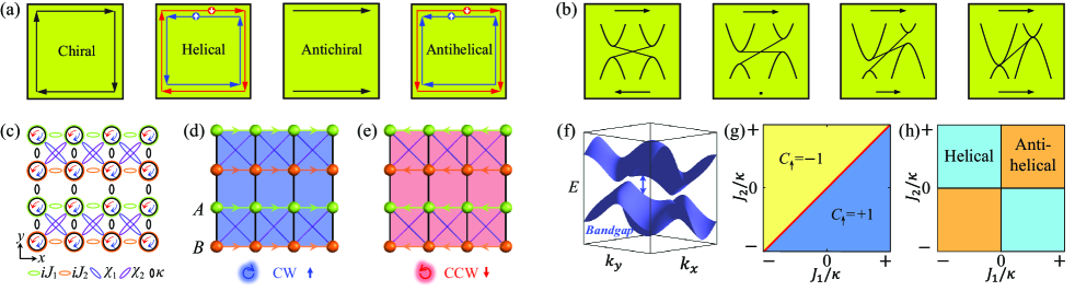
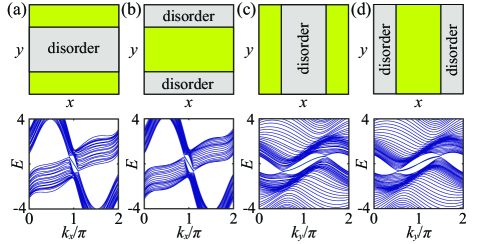
Anisotropic square lattice of ring resonators.—Figure 1(c) presents a two-dimensional anisotropic square lattice of coupled ring resonators (see Supplementary materials A). The clockwise mode (pseudospin-up) and counterclockwise mode (pseudospin-down) are time-reversal counterparts, and they experience the opposite Peierls phases in the horizontal couplings between the nearest-neighbor resonators MHNP11 . The lattice for the pseudospin-up (pseudospin-down) is presented in Fig. 1(d) [Fig. 1(e)]. The horizontal couplings indicated in green and indicated in orange are tunneling-direction-dependent, break the time-reversal symmetry of the Hamiltonian for each individual pseudospin, and separately affect the edge states localized on the upper and lower boundaries. The vertical coupling between the nearest-neighbor resonators is indicated in black. The cross couplings between the next-nearest-neighbor resonators are , LeykamPRL18 . The symmetric component opens a band gap [Fig. 1(f)] and creates a nontrivial topology, whereas the anti-symmetric component affects the band structure, separates the bands in both the and directions, and creates antihelical edge states that are localized on the left and right boundaries in the topological metallic phase.
Topological phases.—The Bloch Hamiltonian for the pseudospin-up is , where is the identical matrix and is the Pauli matrix. The first term adjusts the band energy and the second term determines the band topology. We have and with , . respects the particle-hole symmetry . The topological phase belongs to the class and it is characterized by a topological invariant, that is, the spin-Chern number [Fig. 1(g)]. The band topology is captured by the effective magnetic field . After is substituted with in , the spin-Chern number becomes the definition of a linking number of the two independent periodic vectors and (see Supplementary materials B). is an ellipse that passes through and . is a circle centered at the origin with a fixed radius in the plane. Thus, the two closed curves and are linked when .
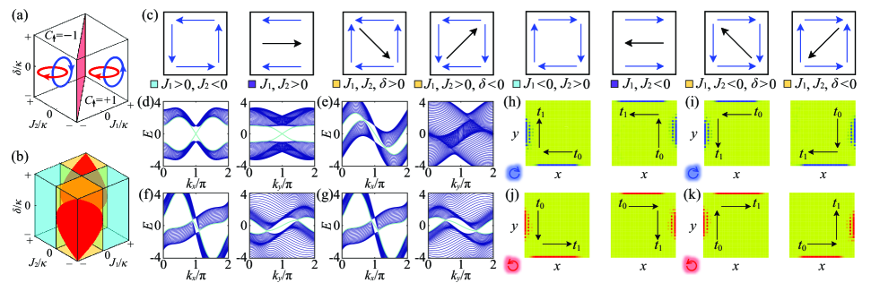
In Fig. 2(a), the red circle that is fixed on the plane is always clockwise; the rotation direction of the blue ellipse reverses along the topological phase transition plane , where the band gap vanishes and becomes coplanar to . The blue ellipse circles counterclockwise around the red circle once in the region (); and the blue ellipse circles clockwise around the red circle once in the region (). The right-hand (left-hand) rule identifies (): orient the thumb pointing along the arrow of the red circle, curl the rest of the fingers pointing along the arrow of the blue ellipse. Notably, in the phase diagram [Fig. 2(b)], two topological phases with opposite spin-Chern numbers have an identical number of edge states.
Antihelical edge states.—Topological edge states appear in the situation that the next-nearest-neighbor coupling is weak than the nearest-neighbor coupling . The nontrivial topology supports helical and antihelical edge states [Fig. 1(h)] that are different from their band structures and their ways of propagation. The antihelical (helical) edge states on the parallel boundaries propagate in the same (opposite) direction, being robust against disorder because of the topological protection and the spatial separation between the edge and bulk states FranzPRL18 .
In Fig. 1(b), the regions are the topological insulating phase; the helical edge states with different pseudospins propagate clockwise or counterclockwise along the lattice boundaries. The topological phase undergoes a metal-insulator phase transition at . The regions are the topological metallic phase KamenevPRL18 ; the edge states excited by the pseudospin-up propagate toward the left (or right) on the two parallel boundaries, but the edge states excited by the pseudospin-down propagate toward the right (or left) boundaries for (or ). These edge states associated with the two pseudospins constitute the antihelical edge states, and the required counterpropagating modes for the antihelical edge states are the bulk states. The bands touch at the topological phase transition, where topological edge states are degenerate and exhibit identical dispersion and propagation velocity.
The square lattice exhibits nontrivial topology throughout the parameter space -- [Fig. 2(a)]. The various types of edge states, as distinguished by their propagation, are presented in Fig. 2(b). The helical edge states are in indicated in cyan and the antihelical edge states are in the other regions . The antihelical edge states differ from the helical edge states in term of their copropagation on the parallel boundaries MHNP11 ; FranzPRL18 . The antihelical edge state excitations with different pseudospins unidirectionally propagate in the opposite directions along the lattice boundaries and enable the separation of the robustly copropagated chiral mode. The helical edge states in the topological insulating phase always appear in both the horizontal and vertical directions; however, the antihelical edge states in the topological metallic phase usually appear only in one direction because of the inseparable band energy in the other direction. Here, the antihelical edge states are simultaneously present in both the horizontal and vertical directions for , where the energy bands are separable in both directions. The antihelical edge states are only present in the horizontal directions for . In Fig. 2(b), the surfaces and divide the parameter space -- into three phases with eight regions. The eight types of edge state propagation for the pseudospin-up excitations are presented in Fig. 2(c). The pseudospin-down edge state excitations propagate in the opposite directions.
The simultaneous sign changes of and reverse the propagation directions of all the antihelical edge states. The four cases of edge modes on the left-half and right-half of Fig. 2(c) propagate in opposite directions. The sign change of only alters the propagation direction of the antihelical edge states in the vertical direction. The antihelical edge states at the strong () pass along the bottom-left and top-right corners and scatter into the bulk at the top-left and bottom-right corners; by contrast, the antihelical edge states at the strong () pass along the bottom-right and top-left corners and scatter into the bulk at the top-right and bottom-left corners. In Fig. 2(c), the helical edge states propagate counterclockwise (clockwise) along the lattice boundaries for () in the cyan region (). The antihelical edge states along the horizontal direction in the red region () of ; the edge state excitation propagates leftward (rightward), scatters into the bulk at the corners, and goes backward. The antihelical edge states are present along both the horizontal and vertical directions when ; the edge state excitation propagates half a closed-loop along the lattice boundaries, scatters into the bulk at the corners, and goes backward along the diagonal direction with the support of the scattering states. The four cases are respectively distributed in the orange regions , , , and of .
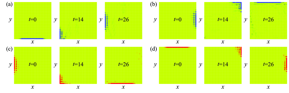
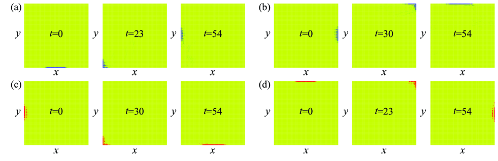
Figures 2(d)-2(g) present the four cases of the band structures for the pseudospin-up presented on the left-half of Fig. 2(c). The propagation of antihelical edge states in Figs. 2(f) and 2(g) for the pseudospin-up are simulated in Figs. 2(h) and 2(i), and the corresponding propagation for the pseudospin-down are simulated in Figs. 2(j) and 2(k). The separation and convergence of different pseudospins toward the opposite corners of the square lattice are observed.
In conclusion, we have introduced the antihelical edge states in the time-reversal symmetric topological metallic phase, and proposed the photonic realization in coupled ring resonators. The antihelical edge states with different pseudospins propagate in the opposite directions along the corners toward the diagonal of the square lattice. Unconventional copropagation is applicable for the robust spin purification. The antihelical edge states become the helical edge states after undergoing a metal-insulator phase transition. The wide range of reconfigurable robust light propagation enables the flexible control of light flow at the edges. Our findings provide insight into the photonic topological metals and are applicable for the acoustic lattices and other two-dimensional metamaterials. Concepts pertaining to topological metals and antihelical edge states are inspiring in the condensed matters and topological materials.
Acknowledgments
This work was supported by National Natural Science Foundation of China (Grants No. 12222504, No. 11975128, and No. 11874225).
Supplementary Materials
.1 A. Experimental realization of the square lattice
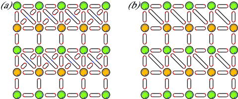
In this section, the experimental realization of the square lattice in the two-dimensional (2D) coupled resonator array is discussed. Figure 3(a) is the schematic of the 2D coupled resonator array. The ring resonators are the primary resonators for the sites of the square lattice. The resonators in green stand for the sites and the resonators in orange stand for the sites . The linking resonators mediate the photons tunneling among the primary resonators and induce the effective couplings between the nearest-neighbor primary resonators and the next-nearest-neighbor primary resonators. The linking resonators and the primary resonators are coupled through their evanescent fields and the coupling strengths depend on the positions between the linking resonators and the primary resonators. For example, the couplings for the CW mode (pseudospin-up) of the primary resonators are mediated by the CCW/CW mode of the linking resonators.
The vertical coupling is reciprocal, the path lengths for the photons tunneling upward and downward between the neighbor ring resonators are equal. The coupling strength is approximately characterized by LYouPRA17 , where and are the hopping and detuning between the primary resonators and the linking resonators; and the frequency of the primary (linking) resonators is ().
The horizontal couplings and are nonreciprocal, carrying the Peierls phase in the couplings. The Peierls phase is implemented through the optical path length difference for the photons tunneling rightward and leftward between the neighbor ring resonators. The CW mode photons tunneling rightward from the lower half of the linking resonator experience an additional path length than the CW mode photons tunneling leftward from the upper half of the linking resonator MHNP11 , where the wave length is . Therefore, the photons tunneling rightward acquire an extra phase factor and the photons tunneling leftward acquire an extra phase factor in the front of the horizontal couplings and .
The cross coupling () between the primary resonators on the diagonal of the square plaquette is directly (indirectly) mediated by the CCW (CW) mode of the linking resonator along the main diagonal of the square plaquette as indicated by the blue (red) arrows. The main diagonal of the square plaquette refers to the line along the upper-left and the lower-right corners of the square plaquette. The cross couplings and are independently mediated through the linking resonators along the diagonals of the square plaquette LeykamPRL18 .
The antihelical edge states can appear in the topological metal phase of the square lattice at the specific case . Thus, the single cross coupling case is adequate for the observation of antihelical edge states in experiments. A concrete system is . In this situation, one of the two cross couplings vanishes as schematically illustrated in Fig. 3(b). This simplifies the setup in the experiment and facilitates the realization of antihelical edge states. The robust propagation with strong can be observed in the situation through switching the orientation of the linking resonator to alter the connection between the nearest-neighbor resonators on the diagonals of the square plaquette. In this manner, the proposed square lattice can alter between two simple situations and .
For example, we consider a simple configuration in experiment that the resonators are neatly arranged in both horizonal and vertical directions of the 2D square lattice. Consequently, the horizontal couplings have equal strengths . A candidate platform for the possible realization of the photonic topological metal and the antihelical edge states can be chosen as follows. In a situation , , , the two cross couplings are , and the cross coupling strength equals to the vertical coupling strength . The round trip length of the resonator is about m. The resonator supports a single mode transverse electric field at the telecom wavelength m HafeziNP13 . The coupling strengths evanescently decay as the width of the air gap between the neighbor resonators; and the coupling strengths approximately decay from to for the air gap width increasing from to HafeZiNP19 . The topologically robust transport can be experimentally implemented in a size square lattice of coupled resonators at the vertical coupling strength , the cross coupling strength , , and the horizontal coupling strengths , . In this situation, the 2D square lattice has a nontrivial topology because of ; and the system is a topological metal hosting the antihelical edge states in both horizontal and vertical directions because of .
.2 B. Spin-Chern number characterized by the linking number of the effective magnetic field
The Chern number characterizes the band topology of the 2D topological phase and the Chern number is proportional to the Hall conductance. In a 2D time-reversal invariant system, although the total Chern number is zero, the spin-Chern numbers are quantized. The spin-Chern number of the lower band for the pseudospin-up (CW) mode is defined by
| (1) |
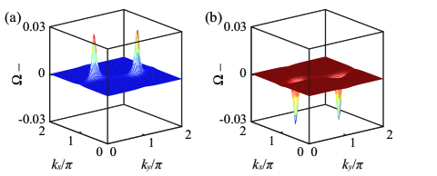
where is the Berry curvature, is the Berry connection, and is the eigenstate of the lower band WGa15 . The spin-Chern number is an integral of the Berry curvature in the entire Brillouin zone (BZ). Figure 4 provides the numerical results of the Berry curvature in the BZ for the topological phases and TFuku05 .
In the following, we explain the relation between the spin-Chern number and the linking number. The spin-Chern number for the two-band Hamiltonian for the pseudospin-up is expressed in the form of QWZPRB06
| (2) |
The effective magnetic field in is with and ; and . Substituting into equation (2), the spin-Chern number is rewritten in the form of
| (3) |
In geometry, equation (3) is the definition of the linking number of two independent closed curves and . The linking number is a topological invariant that characterizes the number of times that and wrap around each other Hannay05 . Thus, the spin-Chern number is equivalent to the linking number of two closed curves and of the effective magnetic field for the pseudospin-up Hamiltonian . The spin-Chern numbers shown in Fig. 4 are in accords with the representative links shown in Fig. 2(a) of the main text.
For the pseudospin-down mode, the signs of the horizontal couplings and change into the opposite and . The Hamiltonian reads . The spin-Chern number obtained from the linking of the effective magnetic field yields . This is straightforward because that the curve and two components of the curve in the and directions are unchanged, and the component of the curve in the direction changes into the opposite.
.3 C. Robustness of the antihelical edge states
In the topological phases of the square lattice, both the helical edge states and the antihelical edge states are topologically-protected and robust to disorder. In comparison, the helical edge states in their propagations are even more stable to the disorder because of the band gap protection. In this section, we provide more details for the robustness of antihelical edge states and their unidirectional propagations in the presence of coupling disorder; notably, the couplings with random disorder satisfy the particle-hole symmetry, which also exists in the square lattice for the pseudospin-up (pseudospin-down). The numerical simulations of the band structures and the robust propagations of antihelical edge states are shown for the imperfect square lattice. The localized edge states and the extended bulk states are spatially separated. Thus, the imperfection in the bulk almost does not affect the edge states and their robust propagations.
The distribution and the localization of the edge states on the boundaries are insensitive to the lattice size; however, the distribution and the extended feature of the bulk states closely depend on the lattice size. The larger lattice size leads to a better spatial separation between the edge states and the bulk states. The influence on the edge states for the disorder in the bulk of the square lattice is slight in comparison with the influence on the edge states for the disorder on the boundaries of the square lattice. This point is elucidated in Fig. 5, where we depict the energy bands for the disorder in the bulk and on the boundaries, respectively; and the random disorder is chosen on all the couplings either inside or outside the central one-half area of the square lattice as schematically illustrated in the upper panels of Fig. 5. The edge states are depicted in Figs. 5(a) and 5(c) for the random disorder in the couplings inside the central one-half area of the square lattice in the bulk; and the edge states are depicted in Figs. 5(b) and 5(d) for the random disorder in the couplings outside the central one-half area of the square lattice on the boundaries. To obtain the 1D projection lattices, the 2D square lattice is set translationally invariant in the () direction for Figs. 5(a) and 5(b) [Figs. 5(c) and 5(d)].
In the numerical simulations, the initial excitation has the Gaussian profile in the form of
| (4) |
where is the edge mode with the momentum or , and . is the center of the wave packet and controls the width of the Gaussian profile. normalizes . The numerical simulations of the robust light propagation for the excitations of antihelical edge states in the presence of random disorder are performed and demonstrated in Fig. 6. All the couplings with random disorder are deviated from the set parameters of the square lattice within the range of . The edge mode excitations robustly propagate along the boundaries. The dynamics in the numerical simulations are close to the dynamics in the absence of disorder exhibited in the main text Fig. 2; this is a consequence of the limited lattice size in the numerical simulations. The robust propagation against disorder is more excellent in the numerical simulations performed in the larger size system as shown in Fig. 7.
In the topological metal phase possessing the antihelical edge states in both the horizontal and vertical directions, there are two types of right-angled ( degrees) corners in the square lattice. One type of corners help the right-angled turning of the edge mode excitations when they propagate along the boundaries; and the other type of corners help the edge mode excitations entering the bulk of the square lattice. Each corner is associated with a cross coupling; and the two types of corners are distinguished from their associated cross couplings and . The formation of the right-angled corners associated with the weak cross coupling enables the degrees turning across the corners for the edge mode excitations propagating along the lattice boundaries. The formation of the right-angled corners associated with the strong cross coupling enables the edge mode excitations entering the bulk of the square lattice.
References
- (1) Lu L, Joannopoulos JD, Soljačić M. Topological photonics. Nat Photonics 2014; 8: 821-9.
- (2) Khanikaev AB, Shvets G. Two-dimensional topological photonics. Nat Photonics 2017; 11: 763-73.
- (3) Ozawa T, Price HM, Amo A, et al. Topological photonics. Rev Mod Phys 2019; 91: 015006.
- (4) Haldane FDM, Raghu S. Possible Realization of Directional Optical Waveguides in Photonic Crystals with Broken Time-Reversal Symmetry. Phys Rev Lett 2008; 100: 013904.
- (5) Wang Z, Chong Y, Joannopoulos JD, et al. Observation of unidirectional backscattering-immune topological electromagnetic states. Nature 2009; 461: 772-5.
- (6) Hafezi M, Demler EA, Lukin MD, et al. Robust optical delay lines with topological protection. Nat Phys 2011; 7: 907-12.
- (7) Fang K, Yu Z, Fan S. Realizing effective magnetic field for photons by controlling the phase of dynamic modulation. Nat Photonics 2012; 6: 782-7.
- (8) Liang GQ, Chong YD. Optical Resonator Analog of a Two-Dimensional Topological Insulator. Phys Rev Lett 2013; 110: 203904.
- (9) Yang HF, Xu J, Xiong ZF, et al. Optically Reconfigurable Spin-Valley Hall Effect of Light in Coupled Nonlinear Ring Resonator Lattice. Phys Rev Lett 2020; 127: 043904.
- (10) Colomés E, Franz M. Antichiral Edge States in a Modified Haldane Nanoribbon. Phys Rev Lett 2018; 120: 086603.
- (11) Zhou P, Liu GG, Yang Y, et al. Observation of Photonic Antichiral Edge States. Phys Rev Lett 2020; 125: 263603.
- (12) Yang Y, Zhu D, Hang Z, et al. Observation of antichiral edge states in a circuit lattice. Sci China Phys Mech Astron 2021; 64: 257011.
- (13) Chen J, Li ZY. Prediction and Observation of Robust One-Way Bulk States in a Gyromagnetic Photonic Crystal. Phys Rev Lett 2022; 128: 257401.
- (14) Leykam D, Mittal S, Hafezi M, et al. Reconfigurable Topological Phases in Next-Nearest-Neighbor Coupled Resonator Lattices. Phys Rev Lett 2018; 121: 023901.
- (15) Ying X, Kamenev A. Symmetry-Protected Topological Metals. Phys Rev Lett 2018; 121: 086810.
- (16) Yang F, Liu YC, You L. Anti- symmetry in dissipatively coupled optical systems. Phys Rev A 2017; 96: 053845.
- (17) Hafezi M, Mittal S, Fan J, et al. Imaging topological edge states in silicon photonics. Nat Photonics 2013; 7: 1001-5.
- (18) Mittal S, Orre VV, Zhu G, et al. Photonic quadrupole topological phases. Nat Photonics 2019; 13: 692-6.
- (19) Gao W, Lawrence M, Yang B, et al. Topological Photonic Phase in Chiral Hyperbolic Metamaterials. Phys Rev Lett 2015; 114: 037402.
- (20) Fukui T, Hatsugai Y, Suzuki H. Chern Numbers in Discretized Brillouin Zone: Efficient Method of Computing (Spin) Hall Conductances, J Phys Soc Jpn 2015; 74: 1674-7.
- (21) Qi XL, Wu YS, Zhang SC. Topological quantization of the spin Hall effect in two-dimensional paramagnetic semiconductors. Phys Rev B 2006; 74: 085308.
- (22) Dennis MR, Hannay JH. Geometry of Călugăreanu’s theorem, Proc R Soc A 2005; 461: 3245-54.