Application of resolved low- multi-CO line modeling with RADEX to constrain the molecular gas properties in the starburst M82
Abstract
The distribution and physical conditions of molecular gas are closely linked to star formation and the subsequent evolution of galaxies. Emission from carbon monoxide (CO) and its isotopologues traces the bulk of molecular gas and provides constraints on the physical conditions through their line ratios. However, comprehensive understanding on how the particular choice of line modeling approach impacts derived molecular properties remain incomplete. Here, we study the nearby starburst galaxy M82, known for its intense star formation and molecular emission, using the large set of available multi-CO line observations. We present high-resolution ( pc) emission of seven CO isotopologue lines, including 12CO, 13CO, and C18O from the , and transitions. Using RADEX for radiative transfer modeling, we analyze M82’s molecular properties with (i) a one-zone model and (ii) a variable density model, comparing observed and simulated emissions via a minimum analysis. We find that inferred gas conditions—kinetic temperature and density—are consistent across models, with minimal statistical differences. However, due to their low critical densities ( cm-3), low- CO isotopologue lines do not effectively probe higher density gas prevalent in starburst environments like that of M82. Our results further imply that this limitation extends to high-redshift () galaxies with similar conditions, where low- CO lines are inadequate for density constraints. Future studies of extreme star-forming regions like M82 will require higher- CO lines or alternative molecular tracers with higher critical densities.
1 Introduction
Cold, dense clouds of molecular gas within the interstellar medium (ISM) serve as the fundamental reservoirs from which stars form in galaxies. The physical and chemical properties of this gas—such as temperatures, densities, and metallicity—play a crucial role in initiating and regulating the star formation process (see reviews by Omont, 2007; Kennicutt & Evans, 2012; Schinnerer & Leroy, 2024). These conditions influence the balance between gravitational collapse and thermal support, which determines the efficiency and timescale of star formation.
One common approach to probing the conditions within molecular gas clouds is through observations of rotational transitions of carbon monoxide (CO) and its isotopologues. The assumption of local thermodynamic equilibrium (LTE) is often employed in these studies, as it simplifies the radiative transfer calculations necessary for deriving physical parameters (Wilson et al., 2009; Cormier et al., 2018; Wang et al., 2023). However, the LTE assumption is frequently inadequate for describing the molecular ISM, where collisional processes and radiative trapping can significantly affect the excitation of molecular lines (Shirley, 2015). Consequently, non-LTE modeling approaches have become increasingly important for accurately constraining the conditions of molecular gas. These methods require observations of multiple CO lines to resolve the degeneracies between various physical parameters, such as densities and temperatures Finn et al. 2021; Teng et al. 2022; Roueff et al. 2024).
Utilizing the large set of seven low- CO isotopologue line observations at the GMC-scale (i.e., 100 pc physical resolution), including new SMA data, this study focuses on the bright, nearby starburst galaxy Messier 82 (M82), located at a distance of approximately Mpc (Freedman et al., 1994). M82 is one of the closest and most studied starburst galaxies, with an infrared luminosity of approximately , making it one of the brightest galaxies observed by the Infrared Astronomical Satellite (IRAS). The central nuclear disk (CND) of M82, spanning about 500 pc, is a region of intense star formation activity. Compared to the Milky Way’s central molecular zone, M82’s CND is 100 times more luminous (Rieke et al., 1980). Given its extreme star-forming environment, M82 also presents a viable analog for high-redshift galaxies.
Numerous studies have targeted CO and other millimeter (mm) line emissions in M82’s CND to explore the properties of its molecular gas. At a coarser angular resolution ( or 350 pc), Petitpas & Wilson (2000) mapped the 3–2 CO isotopologue lines using the JCMT. Their large-velocity-gradient line modeling suggests the presence of even optically thin 12CO(1-0) emission in the central region. At a GMC-scale resolution, early work by Weiß et al. (2001) employed high-resolution (1.5 arcsec, 27pc) observations of the 1–0 12CO, 13CO, and C18O lines to investigate the galaxy’s star formation-driven dynamics. Their study revealed that the kinetic temperature of the molecular gas is elevated in the central region, where star formation is most active, and decreases towards the outer molecular lobes, where star formation rates are lower. However, with only three CO lines observed, the constraints on physical conditions were limited. Subsequent studies have expanded the dataset of CO line observations in M82, employing both LTE and non-LTE modeling techniques to derive more accurate constraints on the physical conditions of the gas. For example, Panuzzo et al. (2010) utilized CO multi-line observations from Herschel Space Telescope to study the molecular gas for a single beam encompassing the entire central region of M82. Their work revealed the presence of a very warm molecular gas component at K.
In this study, we aim to further constrain the resolved molecular gas properties in M82 by analyzing high-resolution low- CO isotopologue observations at 85 pc scale. Specifically, with seven cross-band CO (isotopologue) lines in hand, we set out to benchmark non-LTE modeling of the CO emission with RADEX. We particularly contrast the results derived from assuming a one-zone structure versus a varying density-distribution model to establish how reliable these models are in the context of starburst environments.
This paper is structured as follows: In Section 2, we describe the data used in the study. In Section 3, we present non-LTE radiative transfer modeling techniques and the two approaches we employ to describe the emitting gas. In Section 4, we present the main results, including derived molecular gas properties. We interpret and discuss the results in Section 5. Finally, we present the conclusions in Section 6.
2 Data and Observations
We obtained observations of seven low 12CO (hereafter CO), , and lines with the Submillimeter Array (SMA) and the Northern Extended Millimeter Array (NOEMA). The native angular resolution varies from 2.2 – 4.7, allowing us to resolve the galaxy on a pc physical scale, which corresponds roughly to the typical GMC scale (see Scoville et al., 1987). We provide an overview of the list of observations as well as their characteristics in Table 1.
| Line | Rest Frequency | Angular Scale | Spec. Resolution | Telescope/Reference | Single Dish Available | |
|---|---|---|---|---|---|---|
| [GHz] | [′′]/[pc] | km s-1 | [mK] | |||
| C18O 1–0 | 109.782 | 2.2/40 | 20 | 0.0017 | NOEMA | ✘ |
| 13CO 1–0 | 110.201 | 2.2/40 | 20 | 0.0022 | ✘ | |
| CO 1–0 | 115.271 | 2.1/38 | 5 | 0.014 | ✔ | |
| C18O 2–1 | 219.560 | 4.7/85 | 5 | 0.0039 | SMA | ✔ |
| 13CO 2–1 | 220.399 | 4.2/76 | 5 | 0.0053 | ✔ | |
| CO 2–1 | 230.538 | 3.5/63 | 5 | 0.038 | ✔ | |
| CO 3–2 | 345.796 | 0.8/14 | 5 | 0.17 | ✘ |
Note. — a Channel rms at 5 km s-1 and working resolution (4.7″)
The NOEMA inteferometric data covers the lines of 12CO, 13CO, and C18O. The original data covers an area of 25 arcmin2, extending well beyond the CND of M82 out to 7.9 kpc along the major axis and out to 2.9 kpc along the minor axis. The 12CO(1-0) line has been presented and analyzed in detail in Krieger et al. (2021). We refer to this publication for details on the data calibration and imaging procedures.
In addition, we present new SMA observations as part of this study, including the lines of 13CO, and C18O, and both the and for 12CO. These observations cover only the central CND of M82 and extend to kpc in radius along the major axis of M82. A detailed description of the SMA data reduction and imaging is provided in J. den Brok et al. (in prep.). We provide a short description of the imaging routine in the Appendix A.
Credit for M82 optical Image: NASA, ESA and the Hubble Heritage Team (STScI/AURA). Acknowledgment: J. Gallagher (University of Wisconsin), M. Mountain (STScI) and P. Puxley (NSF).
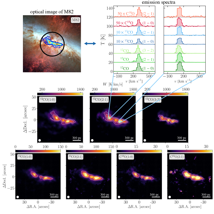
The resulting homogenized data includes the spectral cube and the moment maps derived from it for each line. In Figure 1, we present this data. In the top left corner, we present an HST composite optical image of M82. In the top right corner, we plot the spectra of two lines of sight in the central region, with emission from each isotopologue scaled accordingly for visual purposes. Finally, in the lower panels, we plot moment-0 maps from all lines, convolved to 4.7″and re-sampled on a hexagonal grid. In these maps, bright peaks observed in the CND are clear. These so-called “knots” of emission are consistent with previous observations (see Weiß et al. (2001)).
We note that all of the CO isotopologue line data do not include short-spacing corrections (see Table 3). However, we show in Appendix A that in general only of the flux per line-of-sight is missing, which is well below the assumed flux uncertainty of . Integrated over the entire field of view, the missing flux for the CO isotopologues still remains at for 13CO and C18O (2-1).
3 Multiline Modeling
We use the non-LTE radiative transfer simulation RADEX (van der Tak et al., 2007) to model observed velocity integrated line intensities (in units K km s-1) from and under various environmental conditions, which are described by combinations of density of hydrogen (), kinetic temperature (), 12CO column density per line width (), abundance ratios (), and – for the one-zone model – the beam-filling factor (), assumed to be the same for all lines111We emphasize that the use of a single beam filling factor for the different CO isotopologues is a strong simplification, and can be problematic in the case where selective photodissociation or chemical differentiation leads to a spatial segregation. But stacking results from Galactic clouds (Goldsmith et al., 2008; Pety et al., 2017) reveal a similar distribution and hence motivate the use of a common beam filling factor.. Later, we implement a log-normal distribution for that accounts for a range of densities controlled by distribution width, . We note that incorporating CO isotopologue abundances into RADEX modeling has been shown to improve the recovery of molecular gas physical conditions (Tunnard & Greve, 2016).
RADEX assumes homogeneous gas and solves the radiative transfer equations to find a converged solution for the level population (van der Tak et al., 2007). We use molecular data files from the Leiden Atomic and Molecular Database (Schöier et al., 2005), and we assume the CO isotopologues only collide with because is much more abundant than any other molecule (; Draine 2011).
We consider two models to describe emitting molecular gas, which are described in more details in the following subsections. First, following the common approach in the literature, we assume that the conditions of emitting gas in each line of sight are uniform (i.e. one-zone model). Next, to better describe the gas, we implement a log-normal density model, where follows a log-normal distribution.
For of the sightlines, we notice multiple gas components in the emission spectra. This is expected, as M82 is nearly edge-on. Because the multi-component behavior is not dominant in the central region, we assume a singular component for all sightlines. We note that the solution will be biased towards the brighter component in the case of multiple components, as shown in Teng et al. (2023).
| Model Prescription | Parameter | Range | Stepsize |
| Both Models | Kinetic temperature, | 0.6 – 2.2 | 0.1 dex |
| CO column density, | 16.0 – 19.0 | 0.2 dex | |
| Abundance ratio, | 10 – 200 | 10 | |
| Abundance ratio, | 2 – 20 | 1.5 | |
| Line widtha, | 10 | … | |
| One-zone | Hydrogen volume density, | 2.0 – 5.0 | 0.2 dex |
| Beam-filling factor, | – 0 | 0.2 dex | |
| Log-normal | Mean hydrogen volume density, | 2.0 – 5.0 | 0.2 dex |
| Density distribution width, | 0.2 – 1 | 0.1 |
NOTE – () In essence, RADEX models the line intensities based on the column density per linewidth (). We implement this by allowing a range of column densities but fixing the line width. The derived intensities are consistent upon normalization by the line width.
3.1 One-zone Model
Assuming that the gas in each sightline is uniform, the emission can be described by single values of with the assumption of an identical for all lines. We run RADEX by iterating through the 6 parameters following the ranges and stepsizes outlined in Table 2. The radiative transfer calculations in RADEX depend solely on the ratio, resulting in a degeneracy between and (van der Tak et al., 2007). The RADEX calculations allow us to estimate , which we then multiply by the observed CO(1–0) line width for each pixel to derive the true and thereby avoid this degeneracy. For the model grid, we assume a fixed km s-1 for both models.222We note that this choice is arbitrary, since the results are identical upon normalization by the line width. These parameters generate a six-dimensional (6D) grid, amounting to 12 million points. Our modeling approach and parameter set-up follow those in Teng et al. (2022).
3.2 Log-normal Density Model
Theoretical and observational studies have shown that molecular clouds have a range of densities from diffuse to dense ones, and cannot necessarily be described by a single density as we assumed above (Nishimura et al., 2019). In effort to describe the molecular gas more physically and explore the effects of a more sophisticated model, we implement a log-normal distribution for the density of . The log-normal distribution assumption follows from the literature, which analyzed high resolution observations of molecular cloud in the CO emission (Hughes et al., 2013). Other literature also employed simulations and found a similar log-normal result (see Mac Low & Klessen (2004); Elmegreen (2002); Vazquez-Semadeni (1994)). Following formulations modeling the density of a cloud, we adopt the probability density function (PDF) method used in Leroy et al. (2017a). See more details in Appendix B.
In short, the final intensities are the weighted sum over RADEX one-zone modeled intensities for different volume densities, but for a fixed temperature, abundance, and column density per unit line width. For this calculation, we sum over H2 volume densities ranging from 10-1 to cm-3 in steps of 0.2 dex. Under this model, the final set of parameters governing each line of sight therefore are and , the width of the log-normal density distribution. We note, that strictly speaking, does not correspond to the average volume density introduced for the one-zone model (). For the log-normal model, more precisely corresponds to the mean volume-weighted density. For modeling purposes, we assume a beam filling factor of 1 for all density layers to limit the degrees of freedom. We emphasize that this is a simplification, and in certain extragalactic environments, there might be indeed regions within a beam that do not exhibit the presence of any (CO-rich) molecular gas, hence implying the need for a filling factor. However, in the case of the central region of M82, we find a beam filling factor from the one-zone model that is quite large (0.5). The exact value will be part of a future study where we include more mm molecular line tracers.333A key simplification in our log-normal density model prescription lies in modeling the beam-averaged intensity as a density-weighted sum. In principle, each density layer could have a distinct beam filling factor, which likely depends on the local volume density. A more detailed modeling approach could introduce a global beam filling factor to scale the modeled intensities in equation C1. However, in this study, we refrain from adding this additional free parameter due to the limited number of available lines. While this simplification might introduce a bias, it does not impact the main conclusion: even with a global beam filling factor, the density cannot be reliably constrained above a volume density of cm-3. The ranges through which we iterate can be found in Table 2. More details about the implementation of this density distribution can be found in Appendix B.
3.3 Fitting emission models to observations
We evaluate the goodness of fit of each parameter set or (depending on model) by calculating . To remove nonphysical parameter sets from consideration, we set a prior on the line-of-sight path length (), following Teng et al. (2022), with (where the beam filling factor term is only considered for the one-zone model)
| (1) |
where 500pc is based on the width of M82’s central region.
Assuming a multivariate Gaussian probability distribution, we convert the for each grid point to a probability. Finally, we generate marginalized 1D and 2D likelihood distributions (called PDFs for 1Ds) for every parameter and pair of parameters. These are generated by summing the probability distribution over the full range of parameter(s) except for those of interest. The resulting “1DMax solution” parameter is then selected by determining the highest 1D likelihood for each parameter. More details can be found in Appendix C.
4 Results
In combination, our homogenized dataset consists of 95 sightlines for which all six CO isotopologues lines are detected significantly at S/N5. We note that in this analysis, we exclude the CO (3-2) line due to insignificant emission. More discussions on the inclusion of the line can be found in Subsection 5.1. In the following analysis, we obtain constraints for these 95 sightlines based on our RADEX line modeling. At half beam sampling, given an oversampling factor of , this means we have independent measurements.
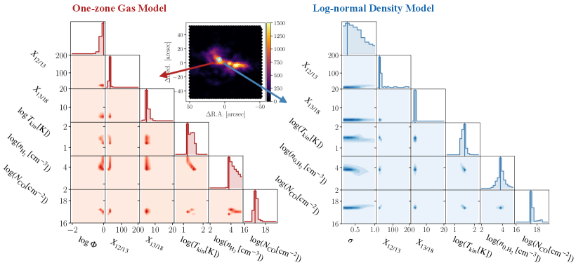
We present the results from our multiline modeling in Figure 2, where we use corner plots to illustrate the PDFs spanning the parameter space. We present corner plots for a single, representative, bright pixel (note that we obtain such corner plots for each individual sightline). The corner plots depict both the 1D and 2D PDFs. The vertical line on the PDFs along the 1D distributions is the 1DMax solution. The statistics of the 1DMax solutions are listed in Table 3. We see the 1D likelihoods of and for the one-zone model are well constrained. For the log-normal model, , and are very tightly constrained as demonstrated by very narrow PDFs. In both models, the PDF is narrow, indicating that is reasonably constrained. In contrast, the parameter is more loosely constrained. For most corner plots, the 1D PDF of is wide, demonstrating an inability to tightly constrain the parameter. This is discussed further in Section 5.1.
4.1 Comparison between one-zone and log-normal derived properties
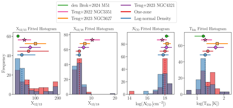
Our two approaches to modeling emitting gas both yield 1DMax solutions for all 6 parameters over the center of the galaxy. In Figure 3, we plot the binned fits of parameters shared between the models, which include , and . We bin the solutions of the 95 sightlines for which we have significant CO isotopologue emission (excluding (3-2)). We see similar behavior when including the 3-2 line, but then being limited to only 34 pixels. We make two notes: first, because we consider the effect of in the one-zone model, the 1DMax value constrained is the sub-beam value, i.e the in the smaller beam described by . In Figure 3, we convert from the sub-beam value to the full-beam value by multiplying by . Second, the values from the two models are not directly comparable because for the log-normal model, is the average density rather than the singular density. It is still instructive, however, to consider their differences.
Figure 3 includes the distribution of the 1DMax solutions. The dotted vertical lines are the medians of the 1DMax solutions over all pixels, and the horizontal markers at the top of the plots indicate the weighted 16th-to-84th percentile range. Above the fits, we show values found in the centers of NGC3627, NGC4321, and NGC3351 which are nearby barred galaxies (Teng et al., 2022, 2023), and the M51 galaxy, which is a nearby grand design spiral galaxy (den Brok et al., 2024). The parameter was not constrained for in den Brok et al. (2024) and thus is left empty in the figure. We see that the two models generally agree for the medians of the , , and parameters. We see that the median of the one-zone values is higher – but within the margin of the scatter – than that of the log-normal model. This likely reflects the fact that in the case of the one-zone model, sub-beam density variations and the resulting CO isotopologue emission are compensated by higher CO isotopologue abundance. In comparison to values found for other galaxies, we see generally more extreme conditions in the barred galaxies and less extreme conditions in M51.
We performed the Kolmogorov-Smirnov (KS) test to quantitatively evaluate the similarity between the results. The p-values from the KS test are listed in Table 3. For 3 of the 5 parameters shared by the models, the p-value was greater than 0.05, indicating that the difference between the results is not statistically significant. For the two parameters where the p-value was found to be , namely and , the medians were verified to be within 0.1 dex.
4.2 Optical Depth Calculation
For each sightline, we derive the line center optical depth of the 1-0 transition of and as follows: for each pixel, we marginalize all modeled optical depths over the whole grid to obtain a 1DMax estimate. We note that in the subsequent section, we work with the optical depths derived from the one-zone model. A similar calculation for the log-normal density model is more ambiguous, since each layer will have a different opacity.
| Model | ||||||||
|---|---|---|---|---|---|---|---|---|
| One-zone | Median | 3.71 | 1.4 | 18.2 | 60.0 | 5.0 | 0.4 | – |
| Mean | 3.4 | 1.65 | 18.46 | 74.84 | 5.3 | 0.59 | – | |
| Std. Dev. | 0.42 | 0.32 | 0.43 | 42.51 | 2.71 | 0.27 | – | |
| Log-normal | Median | 4.2 | 1.3 | 17.80 | 60.0 | 3.5 | – | 0.4 |
| Mean | 4.3 | 1.33 | 17.93 | 70.21 | 3.89 | – | 0.50 | |
| Std. Dev. | 0.56 | 0.19 | 0.44 | 46.07 | 2.63 | – | 0.35 | |
| Comparisona | p-value | 0.095 | 0.099 | 0.99 | – | – |
Note. — (a) We compare the two distributions using the KS statistic.
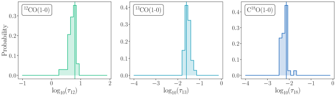
In Figure 4, we bin the 1DMax solutions from each isotopologue. We refer to relative frequency as probability. We find (in the leftmost panel) that the emission is optically thick, as for all sightlines. We note that the derived values also align with those found for the centers of other nearby galaxies, including NGC 3351, 3627, and 4321, using a similar modeling approach (Teng et al., 2022, 2023). In contrast, we note that Petitpas & Wilson (2000) report lower optical depths (around 0.3–3 for 12CO(1-0)). However, these values correspond to measurements at 22″and also depend on the range of assumptions of kinetic temperatures and the CO isotopologue abundances. We note that their optical depths are also above unity if we select their model results which used values for kinetic temperatures (30 K) and 13CO/12CO abundance ratio (70) that are similar to what we report.
We find that the and 1-0 emission is exclusively optically thin with and . This aligns well with our expectations of optically thin and emission based on the measured (2-1)/(1-0) excitation ratios. The mean integrated intensity ratio over the 95 sightlines for 13CO(2-1)/(1-0) is 1.62 and for C18O(2-1)/(1-0) is 2.03. Such high ratios are expected in case both the 1-0 and 2-1 transitions remain optically thin and therefore are consistent with our results from the CO line modeling.
5 Discussion
5.1 Limitations of CO isotopologue model applications
As discussed in Section 4.1, we find that the constraints between the one-zone and log-normal model results do not significantly differ for the volume density, , of H2 and the CO isotopologue abundances.
In principle, we expect the log-normal distribution to more closely trace the true physical conditions of the molecular gas since it adopts a range of densities rather than a single value, as in the one-zone model. Inspecting the individual corner plots, however, we see that there is a sharp cut off for the PDF roughly near cm-3, with the values above being weakly or not constrained. Similarly, for the log-normal distribution, while the volume density seems to be constrained around cm-3, we only get a loose constraint on a wide PDFs. This implies that low CO lines are unable to effectively trace higher gas densities that are most likely present in starburst galaxies. This is consistent with expectations based on the critical density and optical depth effects (Shirley, 2015). Indeed, the CO isotopologues used in the study have critical densities on the order of cm-3, which decrease further by roughly another order of magnitude in the optically thick gas.
Finally, we also note that the two model results show similar distributions of derived molecular gas properties (see Figure 3), despite the simplified assumptions employed for both prescriptions. This suggests that the major limitation is inherent to the general low- CO line ratio modeling approach and only to a lesser degree to simplified assumptions, such as a uniform gas layer (for the one-zone model), or no global beam filling factor for the log-normal density model.
There are several indications that support the presence of high density ( cm-3) and warmer (K) molecular gas in the central region of M82:(i) the molecular gas in starbursts is observed to show densities that are much higher than those found in typical disk galaxies (Jackson et al., 1995; Iono et al., 2007). (ii) observations also suggest that the molecular gas in starbursts is warmer (Bradford et al., 2003; Rangwala et al., 2011). Such high temperatures and densities are consistent with the high (2-1)/(1-0) line ratios observed for the CO isotopologues in M82 (see Section 4.2).
Studies using different molecular gas tracers than the low- CO isotopologues indeed report higher density and temperature gas in the central region of M82. For instance, Panuzzo et al. (2010) rely on higher- CO lines observed with Herschel, including the CO(13-12) and report temperatures in the range of 400–800 K, an order of magnitude higher than the average temperatures we find using the CO line modeling approach. Using the formaldehyde lines as a thermometer, Mühle et al. (2007) also report temperatures of around 200 K for the central region. Previous studies also found densities above 104 cm-3. For instance, using higher critical density tracers, including HCN, CS, and HCO+, Naylor et al. (2010) report average molecular gas densities not in excess of 104.4 cm-3.
Therefore, our results suggest that even with sophisticated modeling approaches incorporating numerous low- CO isotopologue lines, it remains crucial to include higher excitation energy lines (e.g., higher- CO lines beyond the 2–1 transition) and high critical density transitions (e.g., multiple HCN transitions) to achieve robust constraints in extreme environments, such as the central region of M82. Indeed, previous Galactic and extragalactic studies focusing on higher- lines or lines of higher critical density do recover higher volume densities. For instance, studies using Herschel SPIRE/FTS and PACS spectra covering higher- lines of up to , do recover higher temperatures (K) and volume densities ( cm-3) in local active galaxies (Pereira-Santaella et al., 2013, 2014; Mashian et al., 2015) and nearby starbursts (NGC 6240 and Arp 193; Papadopoulos et al., 2014). Similarly, studies including dense gas tracers, such as the rotational HCN and HCO+ lines, also recover and constrain the volume densities and temperatures of a hot (K) and dense ( cm-3) molecular gas component in extreme conditions found in ULIRGs (e.g., Mashian et al., 2015; Imanishi et al., 2023a, b) or other local starbursts (Krips et al., 2008; Greve et al., 2009). These prior findings reinforce our conclusion that relying on low- CO isotopologue transitions alone can lead to an incomplete characterization of molecular gas conditions in extreme environments, such as the central region of M82, and underscore the importance of expanding the range of molecular tracers to capture the varied physical conditions in starbursts.
The intense star formation and high molecular gas densities in M82 serve as a compelling nearby analog to the molecular gas conditions in high-redshift galaxies (; e.g., Weiß et al., 2005; Casey et al., 2014). Our findings underscore the need for caution when interpreting low- CO lines in studies of high- systems. Analyses relying solely on low- transitions risk mis-characterizing the density and excitation properties of molecular gas in these environments. To improve the accuracy and diagnostic power of molecular line studies, future work should prioritize the inclusion of multi-line, multi-tracer modeling and higher-density tracers, particularly in starburst galaxies, both locally and at high redshift.
6 Conclusion
We present analysis of high resolution ( pc physical scale) observations of CO isotopologues from seven different low- transitions across the center of M82. We model emitting molecular gas under two assumptions: one-zone and log-normal density distributions. We use these models together with a non-LTE radiative transfer simulation from RADEX and likelihood analysis to constrain the physical conditions of the molecular gas. We obtain solutions for 95 sightlines within the central (kpc) region of M82. Our main findings are as follows:
-
1.
The derived parameters from the two models, particularly the H2 volume density and relative CO isotopologue abundances, are not statistically significantly different. Moreover, models do not tightly constrain the parameter, which describes the width of the log-normal density distribution.
-
2.
The derived optical depths of the 1-0 transition of 12CO are optically thick and are optically thin for 13CO and C18O for all sightlines. In particular, the optically thin emission for the CO isotopologue lines is expected as their (2-1)/(1-0) line ratios are above unity.
-
3.
While higher- lines are critical to constrain the conditions in particular environments of high densities and temperatures, we find that the CO 3-2 line alone does significantly improve the estimate of molecular gas conditions for most sightlines. Overall, we find that the effectiveness of low- CO isotopologue line modeling might be limited in the case of extreme environments found in starbursts, where gas densities exceed the critical density significantly and the temperatures exceed the excitation temperatures of the lines.
For future work, higher CO lines as well as emission from other molecules with higher critical densities, such as HCN and HCO+ are needed for robust non-LTE analyses of molecular gas.
acknowledgments
We thank the anonymous referee for going carefully through the paper and appreciate their helpful and constructive comments that improved the clarity of this paper. We use data from the Submillimeter Array which is a joint project between the Smithsonian Astrophysical Observatory and the Academia Sinica Institute of Astronomy and Astrophysics and is funded by the Smithsonian Institution and the Academia Sinica. We recognize that Maunakea is a culturally important site for the indigenous Hawaiian people; we are privileged to study the cosmos from its summit. This work is also based on observations carried out under project IDs w18by and 107-19 with the IRAM NOEMA Interferometer and 30m telescope. IRAM is supported by INSU/CNRS (France), MPG (Germany) and IGN (Spain). JdB and EWK acknowledge support from the Smithsonian Institution as Submillimeter Array (SMA) Fellows. MJJD and AU acknowledge support from the Spanish grant PID2022-138560NB-I00, funded by MCIN/AEI/10.13039/501100011033/FEDER, EU.
Appendix A Interferometric SMA data calibration and imaging
The SMA observations of the 2-1 transition of 12CO, 13CO, and C18O were carried out as part of the 2022 SMA Interferometry School (program ID: 2021B-S059; PIs: J. den Brok, C. Eibensteiner, I. Beslic) and a dedicated wide-band SMA survey covering the 200–300 GHz frequency range (program IDs: 2022B-S034, 2023B-S033; PI: J. den Brok). The data calibration and imaging procedures for these observations will be detailed in J. den Brok et al. (in prep.). For completeness, we provide a brief summary of the data reduction and imaging steps here.
A.1 SMA Observations and Data Calibration
The data presented in this project are a combination of observations from three separate tracks carried out on 2022 January 5, 2023 January 24, and 2023 January 25. The 2022 observations, which were part of the SMA Interferometry School program, were obtained in the compact configuration, while the 2023 observations were conducted with the SMA in the subcompact configuration. All tracks were observed under favorable weather conditions, with a nightly average ,mm.
Throughout the observing sessions, we used a set of flux, gain, and bandpass calibrators, selected based on their availability. For all tracks, Uranus was used as the flux calibrator. The gain calibrators, 0958+655 and 0841+708, were observed, as both were sufficiently bright, with a flux density of 0.5 Jy, allowing for efficient calibration with scans of 2 min each. For bandpass calibration, either 0319+415 or 3c84 was selected.
The calibration of the SMA data itself was carried out using the Common Astronomy Software Applications (CASA; CASA Team et al. 2022) package. For this, the raw SMA data were converted to CASA-readable measurement set (MS) files using the pyuvdata (Hazelton et al., 2017) utilities. We then employed the SMA data calibration scripts444https://github.com/Smithsonian/sma-data-reduction to perform the bandpass, gain, and flux calibration.
A.2 SMA Imaging using the PHANGS Imaging Pipeline
Using the calibrated CASA-readable measurement sets, we use the PHANGS-ALMA imaging pipeline (Leroy et al., 2021)555https://github.com/akleroy/phangs_imaging_scripts/ to perform the line imaging. In order for the PHANGS pipeline to work for SMA data, we have to mimic the ALMA format by adding scan intents to the measurement set table. The final imaging is performed using the tclean task from casa. The pipeline performs the continuum subtraction and cleaning automatically. We refer to Leroy et al. (2021) for a detailed description of the functionality and individual steps of the pipeline. We note that we do not reweight the visibilities as the SMA’s weights are well-defined based on system temperature measurements made throughout the observations.
A.3 Assessing the degree of missing flux due to missing short-spacing correction
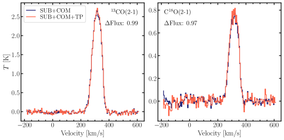
For the NOEMA 3mm 13CO and C18O observations, we lack short-spacing corrected observations. Therefore, for consistency, we also work with the 1.3mm observations before being short-spacing corrected. Using DDT 30m observations (E20-02; PIs: J. den Brok, C. Eibensteiner, I. Beslic), we can assess to what degree the SMA data are affected by the lack of the shortest baselines. In Figure 5, we provide a comparison of the interferometric only (blue) and short-spacing corrected (orange) spectrum extracted along a line of sight in the central molecular region of M82. We find that the difference in integrated intensity is less than 3% for individual sightlines, therefore, the SMA observations appear to recover the significant fraction of the total flux. Integrated over the entire map, the missing integrated flux is still only around 10%.
Appendix B Log-normal Model
The gas density in a molecular cloud is described by
| (B1) |
where is the fraction of molecules with volume densities in a logarithmic step centered on , is the volume density normalized by the mean volume density, , and is the width of the distribution 666Note that the distribution does not peak at the center volume density (), but rather it peaks at ..
The adjusted intensities correspond to the sum of intensities weighted by the volume density PDF at fixed , , and isotopologue abundances as follows:
| (B2) |
Appendix C Matching Observations with Models
For both models, to evaluate the goodness of fit for a parameter set (of structure , where is only considered in the log-normal model), we compute as follows:
| (C1) |
where considers the adjustment of the line width. We use , where the FWHM is the derived moment-2 value. We adjust the modeled intensity by the beam filling factor of the line, , which we vary from 0.01 – 1 in logarithmic steps of 0.2 dex for the one-zone model. We note that, in principle, one could also introduce, similarly, a global beam filling factor for the log-normal density distribution. However, this would introduce an additional free parameter. Therefore, we refer the analysis of the introduction of a global beam filling factor to a future study once more CO isotopologue lines are available. The observational uncertainty is described by the parameter , not to be confused with log-normal distribution width . We additionally apply to the noise uncertainty a conservative estimate of 10% uncertainty on the measured intensity, which is commonly adopted in the literature (e.g., Leroy et al., 2017b; Teng et al., 2022). To quantify the significance of the minimum , we compute for each parameter set a likelihood probability, assuming a multivariate Gaussian probability distribution:
| (C2) |
We compute this probability for each parameter set in the model parameter space, which generates a 6D probability cube. We generate marginalized 1D and 2D likelihood distributions for any given parameter (or pair of parameters) by summing the joint probability distribution over the full range of parameter(s) except the one(s) in question. The resulting “1DMax solution” parameter is then selected by determining the highest 1D likelihood in each parameter. For more details, see Teng et al. (2022).
Appendix D Examining effect of including higher J lines
We examine how effectively CO isotopologue lines can trace more extreme molecular gas conditions, specifically, , a parameter that describes excitation conditions along with . This question has been examined by Teng et al. (2023), who found that for three nearby barred galaxies, including the 3-2 line(s) from CO isotopologues resulted in much less scatter and/or bias when incorporated in the radiative transfer modeling.
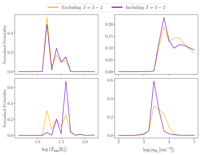
We compare the one-zone model 1D PDFs derived from likelihood analysis including and excluding the 3-2 line. In Figure 6, we plot for two pixels the 1D PDFs for and parameter. These two specific pixels were chosen because they reflect the general behavior we see among all pixels. In purple, we plot the marginalization derived from including the line, and in yellow, we plot the marginalization derived without the line. For the top panel, we see how, both parameters, including the higher line do not change the resulting 1DMax solutions or the overall shape of the 1D PDF significantly. In other words, the 3-2 line does not help constrain the parameters further.
For the bottom panel, we see how the line does not change the 1DMax solution for (most likely due to the low critical density) but it does help trace higher temperatures. While this pixel demonstrates an example where the line aids in tracing more extreme excitation conditions, this behavior is not clear in all pixels. The line, for many pixels, is not effective in tracing the extreme star-forming conditions in the nucleus of M82.
References
- Astropy Collaboration et al. (2013) Astropy Collaboration, Robitaille, T. P., Tollerud, E. J., et al. 2013, A&A, 558, A33, doi: 10.1051/0004-6361/201322068
- Astropy Collaboration et al. (2018) Astropy Collaboration, Price-Whelan, A. M., Sipőcz, B. M., et al. 2018, AJ, 156, 123, doi: 10.3847/1538-3881/aabc4f
- Bradford et al. (2003) Bradford, C. M., Nikola, T., Stacey, G. J., et al. 2003, ApJ, 586, 891, doi: 10.1086/367854
- CASA Team et al. (2022) CASA Team, Bean, B., Bhatnagar, S., et al. 2022, PASP, 134, 114501, doi: 10.1088/1538-3873/ac9642
- Casey et al. (2014) Casey, C. M., Narayanan, D., & Cooray, A. 2014, Phys. Rep., 541, 45, doi: 10.1016/j.physrep.2014.02.009
- Cormier et al. (2018) Cormier, D., Bigiel, F., Jiménez-Donaire, M. J., et al. 2018, MNRAS, 475, 3909, doi: 10.1093/mnras/sty059
- den Brok et al. (2024) den Brok, J., Jiménez-Donaire, M. J., Leroy, A., et al. 2024, arXiv e-prints, arXiv:2410.21399, doi: 10.48550/arXiv.2410.21399
- Draine (2011) Draine, B. T. 2011, Physics of the Interstellar and Intergalactic Medium
- Elmegreen (2002) Elmegreen, B. G. 2002, ApJ, 577, 206, doi: 10.1086/342177
- Finn et al. (2021) Finn, M. K., Indebetouw, R., Johnson, K. E., et al. 2021, ApJ, 917, 106, doi: 10.3847/1538-4357/ac090c
- Freedman et al. (1994) Freedman, W. L., Hughes, S. M., Madore, B. F., et al. 1994, ApJ, 427, 628, doi: 10.1086/174172
- Goldsmith et al. (2008) Goldsmith, P. F., Heyer, M., Narayanan, G., et al. 2008, ApJ, 680, 428, doi: 10.1086/587166
- Greve et al. (2009) Greve, T. R., Papadopoulos, P. P., Gao, Y., & Radford, S. J. E. 2009, ApJ, 692, 1432, doi: 10.1088/0004-637X/692/2/1432
- Harris et al. (2020) Harris, C. R., Millman, K. J., van der Walt, S. J., et al. 2020, Nature, 585, 357, doi: 10.1038/s41586-020-2649-2
- Hazelton et al. (2017) Hazelton, B. J., Jacobs, D. C., Pober, J. C., & Beardsley, A. P. 2017, The Journal of Open Source Software, 2, 140, doi: 10.21105/joss.00140
- Hughes et al. (2013) Hughes, A., Meidt, S. E., Schinnerer, E., et al. 2013, ApJ, 779, 44, doi: 10.1088/0004-637X/779/1/44
- Imanishi et al. (2023a) Imanishi, M., Baba, S., Nakanishi, K., & Izumi, T. 2023a, ApJ, 954, 148, doi: 10.3847/1538-4357/ace90d
- Imanishi et al. (2023b) —. 2023b, ApJ, 950, 75, doi: 10.3847/1538-4357/acc388
- Iono et al. (2007) Iono, D., Wilson, C. D., Takakuwa, S., et al. 2007, ApJ, 659, 283, doi: 10.1086/512362
- Jackson et al. (1995) Jackson, J. M., Paglione, T. A. D., Carlstrom, J. E., & Rieu, N.-Q. 1995, ApJ, 438, 695, doi: 10.1086/175113
- Kennicutt & Evans (2012) Kennicutt, R. C., & Evans, N. J. 2012, ARA&A, 50, 531, doi: 10.1146/annurev-astro-081811-125610
- Krieger et al. (2021) Krieger, N., Walter, F., Bolatto, A. D., et al. 2021, ApJ, 915, L3, doi: 10.3847/2041-8213/ac01e9
- Krips et al. (2008) Krips, M., Neri, R., García-Burillo, S., et al. 2008, ApJ, 677, 262, doi: 10.1086/527367
- Leroy et al. (2017a) Leroy, A. K., Schinnerer, E., Hughes, A., et al. 2017a, ApJ, 846, 71, doi: 10.3847/1538-4357/aa7fef
- Leroy et al. (2017b) Leroy, A. K., Usero, A., Schruba, A., et al. 2017b, ApJ, 835, 217, doi: 10.3847/1538-4357/835/2/217
- Leroy et al. (2021) Leroy, A. K., Hughes, A., Liu, D., et al. 2021, ApJS, 255, 19, doi: 10.3847/1538-4365/abec80
- Mac Low & Klessen (2004) Mac Low, M.-M., & Klessen, R. S. 2004, Reviews of Modern Physics, 76, 125, doi: 10.1103/RevModPhys.76.125
- Mashian et al. (2015) Mashian, N., Sturm, E., Sternberg, A., et al. 2015, ApJ, 802, 81, doi: 10.1088/0004-637X/802/2/81
- Mühle et al. (2007) Mühle, S., Seaquist, E. R., & Henkel, C. 2007, ApJ, 671, 1579, doi: 10.1086/522294
- Naylor et al. (2010) Naylor, B. J., Bradford, C. M., Aguirre, J. E., et al. 2010, ApJ, 722, 668, doi: 10.1088/0004-637X/722/1/668
- Nishimura et al. (2019) Nishimura, Y., Watanabe, Y., Harada, N., Kohno, K., & Yamamoto, S. 2019, ApJ, 879, 65, doi: 10.3847/1538-4357/ab24d3
- Omont (2007) Omont, A. 2007, Reports on Progress in Physics, 70, 1099, doi: 10.1088/0034-4885/70/7/R03
- Panuzzo et al. (2010) Panuzzo, P., Rangwala, N., Rykala, A., et al. 2010, A&A, 518, L37, doi: 10.1051/0004-6361/201014558
- Papadopoulos et al. (2014) Papadopoulos, P. P., Zhang, Z.-Y., Xilouris, E. M., et al. 2014, ApJ, 788, 153, doi: 10.1088/0004-637X/788/2/153
- Pereira-Santaella et al. (2014) Pereira-Santaella, M., Spinoglio, L., van der Werf, P. P., & Piqueras López, J. 2014, A&A, 566, A49, doi: 10.1051/0004-6361/201423430
- Pereira-Santaella et al. (2013) Pereira-Santaella, M., Spinoglio, L., Busquet, G., et al. 2013, ApJ, 768, 55, doi: 10.1088/0004-637X/768/1/55
- Petitpas & Wilson (2000) Petitpas, G. R., & Wilson, C. D. 2000, ApJ, 538, L117, doi: 10.1086/312816
- Pety et al. (2017) Pety, J., Guzmán, V. V., Orkisz, J. H., et al. 2017, A&A, 599, A98, doi: 10.1051/0004-6361/201629862
- Rangwala et al. (2011) Rangwala, N., Maloney, P. R., Glenn, J., et al. 2011, ApJ, 743, 94, doi: 10.1088/0004-637X/743/1/94
- Rieke et al. (1980) Rieke, G. H., Lebofsky, M. J., Thompson, R. I., Low, F. J., & Tokunaga, A. T. 1980, ApJ, 238, 24, doi: 10.1086/157954
- Roueff et al. (2024) Roueff, A., Pety, J., Gerin, M., et al. 2024, A&A, 686, A255, doi: 10.1051/0004-6361/202449148
- Schinnerer & Leroy (2024) Schinnerer, E., & Leroy, A. K. 2024, arXiv e-prints, arXiv:2403.19843, doi: 10.48550/arXiv.2403.19843
- Schöier et al. (2005) Schöier, F. L., van der Tak, F. F. S., van Dishoeck, E. F., & Black, J. H. 2005, A&A, 432, 369, doi: 10.1051/0004-6361:20041729
- Scoville et al. (1987) Scoville, N. Z., Yun, M. S., Clemens, D. P., Sanders, D. B., & Waller, W. H. 1987, ApJS, 63, 821, doi: 10.1086/191185
- Shirley (2015) Shirley, Y. L. 2015, PASP, 127, 299, doi: 10.1086/680342
- Teng et al. (2022) Teng, Y.-H., Sandstrom, K. M., Sun, J., et al. 2022, ApJ, 925, 72, doi: 10.3847/1538-4357/ac382f
- Teng et al. (2023) —. 2023, ApJ, 950, 119, doi: 10.3847/1538-4357/accb86
- Tunnard & Greve (2016) Tunnard, R., & Greve, T. R. 2016, ApJ, 819, 161, doi: 10.3847/0004-637X/819/2/161
- van der Tak et al. (2007) van der Tak, F. F. S., Black, J. H., Schöier, F. L., Jansen, D. J., & van Dishoeck, E. F. 2007, A&A, 468, 627, doi: 10.1051/0004-6361:20066820
- Vazquez-Semadeni (1994) Vazquez-Semadeni, E. 1994, ApJ, 423, 681, doi: 10.1086/173847
- Wang et al. (2023) Wang, C., Feng, H., Yang, J., et al. 2023, AJ, 166, 121, doi: 10.3847/1538-3881/acebdd
- Weiß et al. (2001) Weiß, A., Neininger, N., Hüttemeister, S., & Klein, U. 2001, A&A, 365, 571, doi: 10.1051/0004-6361:20000145
- Weiß et al. (2005) Weiß, A., Walter, F., & Scoville, N. Z. 2005, A&A, 438, 533, doi: 10.1051/0004-6361:20052667
- Wilson et al. (2009) Wilson, T. L., Rohlfs, K., & Hüttemeister, S. 2009, Tools of Radio Astronomy (Springer), doi: 10.1007/978-3-540-85122-6