Applications of a space-time FOSLS formulation
for parabolic PDEs
Abstract.
In this work, we show that the space-time first-order system least-squares (FOSLS) formulation [Führer, Karkulik, Comput. Math. Appl. 92 (2021)] for the heat equation and its recent generalization [Gantner, Stevenson, ESAIM Math. Model. Numer. Anal. 55 (2021)] to arbitrary second-order parabolic PDEs can be used to efficiently solve parameter-dependent problems, optimal control problems, and problems on time-dependent spatial domains.
Key words and phrases:
Parabolic PDEs, space-time FOSLS, reduced basis method, optimal control problems, time-dependent domains2010 Mathematics Subject Classification:
35K20, 49J20, 65M12, 65M15, 65M601. Introduction
It is well-known, e.g., from [Wlo87, SS09], that the operator corresponding to the heat equation , on a time-space cylinder , where and , with homogeneous Dirichlet boundary conditions, is a boundedly invertible linear mapping between and , where and . For source term and initial data , the recent work [FK21] has proven that
where equipped with the graph norm, is a well-posed first-order system least-squares (FOSLS) formulation for the pair of the solution and (minus) its spatial gradient . This formulation can already be found in [BG09] without a proof of its well-posedness though. In [GS21], we have generalized the result to second-order parabolic PDEs with arbitrary Dirichlet and/or Neumann boundary conditions (in the case of inhomogeneous boundary conditions appending a squared norm of a boundary residual, which is not of -type, to the least-squares functional). In particular, we have shown that source terms are covered and in the definition of may be replaced by . We also mention our recent generalization to the instationary Stokes problem with so-called slip boundary conditions [GS22a].
Compared to other space-time discretization approaches such as [And13, Ste15, LMN16, SW21b, SW21a], the FOSLS formulation has the major advantage that it results in a symmetric, and, w.r.t. a mesh-independent norm, bounded and coercive bilinear form so that the Galerkin approximation from any conforming trial space is a quasi-best approximation from that space. At least for homogeneous boundary conditions, the minimization is w.r.t. -norms, so that the arising stiffness matrix is sparse and can be easily computed. Moreover, the least-squares functional provides a reliable and efficient a posteriori estimator for the error in the -norm. One disadvantage of the FOSLS method from [FK21, GS21] is that the latter norm for the error in the pair appears to be considerably stronger than the -norm for the error in . Indeed, for standard Lagrange finite element spaces applied to non-smooth solutions, e.g., as those that result from a discontinuity in the transition of initial and boundary data, relatively low convergence rates are reported in [FK21], even when adaptive refinement is employed. This issue shall be addressed in our future work [GS22b] by constructing more suitable trial spaces.
In the present work, we exploit the aforementioned advantages of the FOSLS method to efficiently solve parameter-dependent problems, optimal control problems, and problems on time-dependent spatial domains.
1.1. Parameter-dependent problems
We consider a reduced basis method, where in a potentially expensive offline phase a basis of (highly accurate approximations of the) solutions corresponding to a suitable finite subset of the parameter space is computed so that in the subsequent online phase the solution for arbitrary given parameters can be efficiently approximated from the spanned reduced basis space.
Compared to reduced basis methods based on time stepping and proper orthogonal decomposition (POD), e.g., [HO08, EKP11, Haa17], reduced basis methods based on simultaneous space-time discretization, e.g., [UP14, Yan14, YPU14], yield not only a dimension reduction in space but in space-time; see the comparison in [GMU17]. Consequently, in any case the resulting online phase can be expected to be more efficient.
As already mentioned, compared to other space-time discretization approaches, the FOSLS formulation has the advantage that it results in a coercive bilinear form. In this setting the strongest theoretical results for the reduced basis method are available (see, e.g., [Haa17]), and the construction of the reduced basis does not need to be accompanied by the construction of a corresponding test space that yields inf-sup stability.
Finally, the reliable and efficient a posteriori error estimator of the FOSLS formulation is beneficial for both building the reduced basis and for certification of the obtained approximate solution in the online phase.
1.2. Optimal control problems
We consider a large class of optimal control problems constrained by second-order parabolic PDEs. This includes controls of the source term in or in and of the initial data in as well as desired observations of the PDE solution in , its spatial gradient in , or its restriction to the final time point in .
It is well-known that optimal control problems can be equivalently formulated as saddle-point problem; see, e.g., [Lio68]. The saddle-point formulation is a coupled system of the primal equation and some adjoint equation. When solving it iteratively, e.g., by a gradient descent method [Trö10, HPUU08], the approximate solutions are required over the whole space-time cylinder and not just at the final time point. This nullifies the potential advantage of time-stepping methods such as [MV07, MV08], which in the case of a forward problem only need to store the approximation at the current time step.
Instead space-time methods such as [GHZ12, LSTY21b, LSTY21a, LS21] aim to solve the saddle-point problem at once on some mesh of the space-time cylinder . All of the mentioned works consider optimal control problems constrained by the heat equation with control of the source term and desired observation of the PDE solution itself. In contrast to time-stepping methods, all of them allow for locally adapted meshes because the involved bilinear forms are coercive or inf-sup stable. However, only [GHZ12], which reformulates the problem as a system of fourth order in space and second order in time requiring additional regularity, yields quasi-optimal approximations in the usual sense with the same norm on both sides, as for the others the norms in which the bilinear forms are continuous differ from the norms in which they are coercive or inf-sup stable.
In our approach, we consider the saddle-point problem when the parabolic PDE is replaced by the equivalent FOSLS. Coercivity of the latter implies that this saddle-point problem is for arbitrary discrete subspaces uniformly inf-sup stable and continuous w.r.t. the same norm so that quasi-optimality in the usual sense is valid. We also provide one reliable and one efficient a posteriori error estimator for our method. Other estimators have been derived in [GHZ12, LS21] for the respective methods.
1.3. Time-dependent domains
Finally, we consider second-order parabolic PDEs on time-dependent domains. While this poses a technical difficulty for time-stepping methods [GS17, FR17, LO19, SG20, FS22], in principle, space-time methods [Leh15, HLZ16, LMN16, Moo18, BHT22] can be readily applied because the overall space-time domain remains fixed.
We show that this is indeed the case for the FOSLS method [FK21, GS21] verifying its well-posedness. The analysis requires minimal regularity assumptions on the mapping describing the motion of the spatial domain throughout time. However, we emphasize that our method ultimately only requires a mesh of the space-time domain. This is in contrast to the so-called arbitrary Lagrangian-Eulerian (ALE) time-stepping methods [SHD01, GS17, SG20], which solve the problem on the transformed time-independent domain and thus explicitly involve the mapping. Moreover, our method again allows for arbitrary discrete trial spaces and immediately provides an a reliable and efficient a posteriori error estimator.
1.4. Outline
In Section 2, we fix the general notation (Section 2.1) and recall the formulation of general second-order parabolic PDEs as a first-order system (Section 2.2). In Section 3, we introduce a corresponding reduced basis method for parameter-dependent problems (Section 3.1), discuss the generation of a suitable basis (Section 3.2), and provide a numerical experiment (Section 3.3). In Section 4, we show that the formulation of optimal control problems constrained by the first-order system as a saddle-point problem is uniformly stable for arbitrary trial spaces (Section 4.1), derive an optimality system of PDEs for a certain class of optimal control problems (Section 4.2), which is then used to derive a posteriori error estimators (Section 4.3), and provide two numerical experiments (Section 4.4), where we also demonstrate optimal convergence rate for piecewise linear trial functions if both the optimal control and the corresponding state are sufficiently smooth. In Section 5, we show that the formulation of general second-order PDEs on time-dependent domains as first-order system induces, as for time-independent domains, a linear isomorphism and provide two numerical experiments (Section 5.2). Finally, we draw some conclusion in Section 6.
2. Preliminaries
2.1. General notation
In this work, by we will mean that can be bounded by a multiple of , independently of parameters on which and may depend. Obviously, is defined as , and as and .
For normed linear spaces and , we will denote by the normed linear space of bounded linear mappings . For simplicity only, we exclusively consider linear spaces over the scalar field .
2.2. Formulation of parabolic PDEs as first-order system
Let , , be a Lipschitz domain with boundary , and a given end time point with corresponding time interval . We abbreviate the space-time cylinder with lateral boundary . We consider the following parabolic PDE with homogeneous Dirichlet boundary conditions
| (2.1) |
Here, we will require that is uniformly positive, , and . For unique existence of a (weak) solution of (2.1), we recall the following theorem from, e.g., [SS09, Theorem 5.1].
Theorem 2.1.
With , ,
and for all , the mapping
is a linear isomorphism. In particular, there exists a unique such that
| (2.2) |
Any can be written as
| (2.3) |
for some and , where for . With such a decomposition, and , (2.2) is equivalent to the first-order system111The system studied in [GS21] leads to (2.10) by pre-multiplication with , which is a linear isomorphism on the space defined in (2.12).
| (2.10) |
as is shown in the next theorem.
Theorem 2.2 ([GS21, Theorem 2.3 and Proposition 2.5]).
Notice that is equivalent to the variational problem
Since the bilinear form at the left-hand side is bounded, symmetric and coercive, it provides the ideal setting for the application of Galerkin discretizations. The Galerkin solution from the employed trial space is a quasi-best approximation to w.r.t. . For any approximation of we have the computable a posteriori error estimator . Moreover, the following lemma shows that .
Lemma 2.3 ([GS21, Lemma 2.2]).
The mapping belongs to .
Finally in this section, we provide more information about the splitting (2.3).
3. Parameter-dependent problems
In this section, we consider coefficients and right-hand side that depend additionally on a tuple of parameters in a set . We assume that the coefficients and the right hand sides are parameter-separable in the sense that
| (3.1) |
for some functions and and . Let be some given quantity of interest that is also parameter-separable, i.e., with and . After a possibly computationally expensive offline phase, we want to be able to instantly compute an approximation of for different in the so-called online phase.
3.1. Reduced basis method
Given some parameter , the idea of the reduced basis method is to compute an approximation of from the (low-dimensional) span of some snapshots .
Instead of , very accurate approximations thereof are computed in the offline phase. We will choose as the best approximation to w.r.t. from some high-dimensional subspace , i.e., as the solution of the Galerkin system for all . One easily checks that the parameter-separability (3.1) of the coefficients and the right-hand sides implies parameter-separability of the bilinear form
the linear form
and the squared norm
where again , and each is a continuous bilinear form and each is a continuous linear form. Besides the functions , which form the reduced basis, in the offline phase we further compute the matrices and vectors
In the online phase, we compute as the best approximation to w.r.t. from the span of the reduced basis, i.e., as the solution of a low-dimensional Galerkin system. Assuming that the snapshots , are linearly independent, the corresponding coefficient vector of with respect to this basis is just given by
We stress that the computational effort to solve this linear system depends only on and not on as the involved matrices and vectors have been already computed in the offline phase. Then, the quantity of interest is given by
Again, the involved vectors have been precomputed in the offline phase. Finally, we can even instantly estimate the discretization error in the online phase by
The constants hidden in the -symbol depend only on the -norms of the coefficients and the smallest eigenvalue of .
3.2. Basis generation
It remains to explain how to determine a suitable reduced basis , . Given some sufficiently large training set and some tolerance , we employ a greedy algorithm that starting with , , iteratively adds the snapshot
to the reduced basis and increments by one until
Note that this procedure terminates at most after steps and provides indeed a basis if the discretization error in is negligible. For possible choices of the training set , we refer, e.g., to [Haa17, Remark 2.44].
3.3. Numerical experiment
We consider the example from [GMU17]: Let and . We consider the parameter set with , , and . Moreover, we choose the right-hand sides , , and independently of the parameters with
on the space-time cylinder , , and on , which corresponds to the solution .
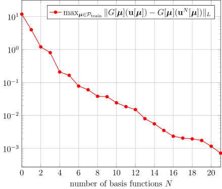
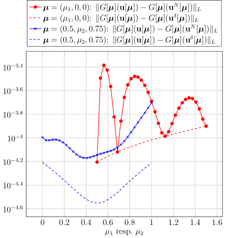
We divide both and into subintervals and choose to be the -fold Cartesian product of continuous piecewise bi-cubic functions333The reason why we consider bi-cubic instead of bi-affine elements as in [GMU17] is that we measure in a stronger norm but still want the approximation error in the space to be negligible., with the first coordinate space restricted by homogeneous Dirichlet boundary conditions on . The training set is chosen as equidistantly distributed points in in each direction, and the tolerance is chosen as . Figure 3.1 displays the approximation error throughout the greedy algorithm of the offline phase with the final , where the -axis is scaled logarithmically. As expected from [BCD+11], we observe exponential convergence. In Figure 3.2, we plot the discretization error of the reduced basis method applied for in the test sets and . For comparison, we also plot the best possible error that one could hope for with the reduced basis method. Although the greedy algorithm only guarantees that these errors are below on the training set , this bound appears to hold also true on the considered test sets.
While a fair comparison to the space-time results of [GMU17] is hard, we only mention that the considered errors, although measured in the stronger norm , are of similar magnitude as the errors of [GMU17] measured in (an approximation of) the norm . The number of reduced basis functions to achieve an accuracy of in [GMU17] is given by . It is also notable that, in contrast to the estimator of [GMU17], which is based on the residual corresponding to (the first components of) , the estimator considered here is provably equivalent to the actual norm of the error and can also be efficiently computed in the online phase.
4. Optimal control problems
Let be fixed, and let be a Hilbert space that is continuously embedded in . We consider (2.10) with , where is a control variable. The corresponding solution is then called state. For being a further Hilbert space, , desired observation , and a parameter , we want to minimize the functional
| (4.1a) | |||
| over | |||
| (4.1b) | |||
Remark 4.1.
Let for some and for some continuously embedded subspace of . Then, (4.1) is equivalent to minimizing
| (4.2a) | |||
| over | |||
| (4.2b) | |||
Indeed, from Theorem 2.2 we know that for , is in the set (4.2b) if and only if with is in the set (4.2b). Knowing that for any , and conversely, any can be written as , where, as shown in Remark 2.4, for the pair with smallest it holds that , the proof of equivalence of (4.1) and (4.2) is completed.
4.1. Formulation as saddle-point problem
Writing (2.10) with right-hand side as for all , and introducing the bilinear forms
and the linear forms
for and , and noting that the constant term in can be neglected for minimization, the optimal control problem (4.1) can be rewritten as
| (4.3) |
The following lemma implies well-posedness and equivalence to a saddle-point problem.
Lemma 4.2.
Let and be arbitrary Hilbert spaces, , , , arbitrary bounded bilinear forms such that and are coercive, is positive semi-definite, and , are bounded linear forms. Then there exists a unique that solves the saddle-point problem
| (4.4) |
and
| (4.5) |
with a constant that depends only on the continuity constants of and the coercivity constants of .
Assuming symmetry of and , the pair is the unique solution of (4.3). In this setting, is known as the co-state.
Proof.
For the first statement, we only have to show that the bilinear form is coercive on the kernel of the operator defined by , and that there holds the LBB (Ladyshenskaja–Babuška–Brezzi) condition
Choosing as well as , coercivity of gives the latter inequality. To see coercivity on the kernel, let with for all . Then, coercivity of and continuity of yield that
or . With positive semi-definiteness of and the coercivity of , we conclude that
and thus the proof of the first statement.
One easily verifies that (4.3) has a unique solution that, assuming symmetric and , solves for all , and for all for which for all . It is known that thanks to the LBB condition, these both equations uniquely determine the first two components of the solution of (4.4), which proves the second statement. ∎
Clearly, Lemma 4.2 is also applicable for arbitrary closed subspaces and with the same uniform constant . In particular, there exists a unique corresponding Galerkin solution of (4.4), which is even quasi-optimal, i.e.,
| (4.6) | ||||
where is proportional to the product of and the maximum of the continuity constants of , , , and (see, e.g., [SW21b, Rem. 3.2]). Fixing the parabolic PDE (2.1), the spaces and , and the mapping , from one infers that , and (see, e.g., [EG21b, Thm. 49.13]), and thus
4.2. Optimality system of PDEs
Let , so that is a Gelfand triple, let be the orthogonal projector onto , , and let be such that .
Then the first equation in (4.4) reads as
i.e., and with and the Hilbert adjoints of and , respectively. Together with , this last equation forms the coupled optimality system associated to our optimal control problem.
To derive a first-order PDE for , we consider the case that
| (4.7) |
for some , , possibly with one or more being zero. We further make the additional regularity assumption . With the outer normal vector on , (formal) integration-by-parts shows that
| (4.8) |
From for all , we infer that , and
| (4.9) |
i.e., is the solution of a backward parabolic problem.
4.3. A posteriori error estimation
The well-posedness of (4.4) shows that for being its solution, and any ,
| (4.10) |
from being a linear isomorphism. The hidden constants absorbed by the two -symbols can be quantified in terms of the well-posedness of (4.4) and that of .
The second term in (4.10) is computable, and in any case when the topology of equals that of and the application of is computable, so is the third. To estimate the first term, we briefly discuss two possibilities.
Remark 4.3.
For the case that and , a functional estimator was introduced in [LS21]. For arbitrary approximations of the state and the co-state , this estimator is a computable guaranteed upper bound for the error in the -norm.
4.3.1. A reliable estimator
We consider the case that is of the form given in (4.7) and abbreviate . In view of (4.8)–(4.9), any (sufficiently smooth) with and provides the upper bound
Choosing as the solution of (4.9) with replaced by the computable approximation , only the term would be present in the upper bound, as then . In this case, the term would even be a reliable and efficient estimator for the first term in (4.10). However, in general the mentioned solution is not computable so that one has to approximate it, e.g., by a Galerkin method. Inspired by [LS21], a computationally cheaper option would be to simply post-process to obtain , i.e., apply a suitable smoothening quasi-interpolator to the in general non-smooth .
4.3.2. An efficient estimator
A computable efficient estimator is obtained by replacing the supremum over in the first term in (4.10) by a supremum over a finite-dimensional subspace . Since for being the Galerkin solution of (4.4) from , the numerator in the first term vanishes for , needs to be a ‘sufficient’ enlargement of .
The resulting estimator can be proven to be even equivalent to the error whenever there exists a projector , bounded uniformly in , with and for all and . For being a finite element space with respect to a general partition of , i.e., not being a product of partitions of and , the construction of such ‘Fortin’ projectors however seems hard.
4.4. Numerical experiments
We consider the heat equation, i.e., , , and in (2.1). Moreover, we set , , , . In particular, with the optimal control problem (4.1) in strong form reads as
| (4.11) |
In this case, the optimality system derived in Section 4.2 reads as
and
where , , and . By prescribing arbitrary , with , , , on , and , the parameters , , and are determined by the optimality system.
The control and co-state are determined by and , i.e.,
and .
Given some conforming quasi-uniform partition of the space-time cylinder into -simplices, we take to be the -fold Cartesian product of continuous piecewise affine functions with the first-coordinate space restricted by homogeneous Dirichlet boundary conditions on , and being the space of piecewise constants.
Taking sufficiently smooth and , in view of (4.6) for the Galerkin solution , we obtain assuming that .
Concerning the latter, assuming the compatibility conditions , , and , [Wlo87, Theorem 27.2] shows that . For a smooth or convex , by interchanging and , from regularity of the Poisson problem shows that , i.e., . For a smooth , from , regularity of the Poisson problem shows that . For being a square, the latter should be read as for any ([Kon70], cf. also [Hac92, Ex. 9.1.25]). Pretending that , we conclude that and , so that , which is thus only ‘nearly’ demonstrated for being a square.
4.4.1. Experiment in 1+1D
Let , , and . We prescribe
on the space-time cylinder , and determine , , and by the optimality system.
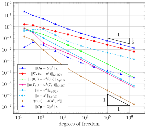
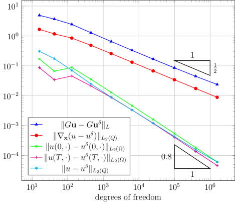
Starting on an initial triangulation of with two elements, we define a sequence of uniform triangulations by splitting all elements in the previous into four new elements by repeated newest vertex bisection. The convergence plot for the resulting Galerkin approximations of (4.4) is displayed in Figure 4.1. While, as expected, and converge at rate , , , , and even converge with the double rate.
4.4.2. Experiment in 2+1D
Let , , and . We prescribe
on the space-time cylinder , and we choose , , and by the optimality system.
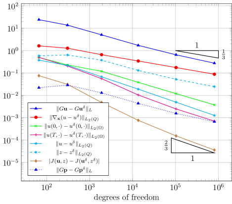
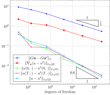
Starting on an initial triangulation of with elements, we define a sequence of quasi-uniform triangulations by splitting all elements in the previous into eight new elements by repeated newest vertex bisection. The convergence plot for the resulting Galerkin approximations of (4.4) is displayed in Figure 4.2. While, as expected, and converge at rate , , , , and even converge (at least almost) with the double rate.
5. Time-dependent domains
In this section, we assume that the spatial domain changes throughout time. More precisely, let be a Lipschitz domain with boundary , and the corresponding space-time cylinder with lateral boundary . We denote the spaces , , , and on by , , , and , respectively. We suppose that the actual space-time domain is given via a bijection of the form
where, for all , maps bijectively onto some Lipschitz domain . We require the regularities , , , and . Note that
| (5.3) |
With the lateral boundary and , we consider the parabolic PDE (2.1) with uniformly positive, , , , , and .
5.1. Formulation as first-order system
As in the time-independent domain case, in first-order system formulation (2.1) reads as
| (5.10) |
which is again well-posed:
Theorem 5.1.
With and defined as in the time-independent domain case444Setting equipped with the norm ., is a linear isomorphism from to .
Proof.
We show that with linear isomorphisms , and .
We set . A familiar property of the Piola transformation (e.g. [EG21a, Lemma 9.6]) is that
| (5.11) |
By definition of we have
| (5.12) |
Applications of the product and chain rules show that
| (5.13) |
We conclude that and thus that is a linear isomorphism.
Remark 5.2.
Assume that also for all . Given , then solves (5.10) if and only if solves
and . Indeed, together with (5.3), (5.12), and Lemma 2.3 imply that , and thus by the additional regularity assumption that . The remainder follows from partial integration. In particular, also the second part of Theorem 2.2 holds analogously for time-dependent domains. Together with the open mapping theorem, this insight also allows to generalize Theorem 2.1.
Theorem 5.1 shows that also in the time-dependent domain case one can approximate the solution of the parabolic PDE by applying a Galerkin discretization to the variational problem for all . Thinking of finite element discretizations, in particular for polytopal domains , this provides an attractive alternative to discretizations that require a transformation of the PDE to a time-independent domain, e.g., ALE time-stepping methods [SHD01, GS17, SG20].
5.2. Numerical experiments
We consider the heat equation, i.e., , , and in (2.1). Moreover, we set and . We will approximate the latter function in the conforming subspace of continuous piecewise affine functions on triangulations of the space-time cylinder whose first component vanishes on the lateral boundary . Using that , we know that for sufficiently smooth and uniform mesh-refinement.


5.2.1. Experiment in 1+1D
Let
where denotes the interior of a set and denotes the convex hull of a set of points; see Figure 5.1 for an illustration. With the bijection , we prescribe the solution by
and choose , and .
Starting on an initial triangulation of with six elements (such that each element is either in or ), we define a sequence of triangulations by splitting all elements in the previous into four new elements by repeated newest vertex bisection. We compute the Galerkin approximation of with respect to the scalar product , with being the -fold Cartesian product of continuous piecewise affine functions on whose first component vanishes on . The corresponding convergence plot is displayed in Figure 5.2. Here, denotes the first component of . While and converge as expected at rate , , , and converge roughly with the rate .
5.2.2. Experiment in 2+1D
Let
where denotes the interior of a set and denotes the convex hull of a set of points; see Figure 5.1 for an illustration. With the bijection , we prescribe the solution by
and choose , and .
Starting on an initial triangulation of with twelve elements (such that each element is either in or ), we define a sequence of triangulations by splitting all elements in the previous into eight new elements by repeated newest vertex bisection. We compute the Galerkin approximation of with respect to the scalar product , with being the -fold Cartesian product of continuous piecewise affine functions on whose first component vanishes on . The corresponding convergence plot is displayed in Figure 5.3. Here, denotes the first component of . While and converge as expected at rate , , , and converge roughly with the rate .
6. Conclusion
In this work, we have demonstrated that the space-time FOSLS [FK21] and its generalization [GS21] to general second-order parabolic PDEs can be easily applied to solve parameter-dependent problems, optimal control problems, and time-dependent domain problems. In each case, completely unstructured space-time finite elements may be employed, and our numerical experiments exhibit optimal convergence. We also want to stress that the FOSLS is applicable to the combined problem, i.e., parameter-dependent optimal control problems on time-dependent domains. Indeed, the inf-sup stability of the saddle-point problem corresponding to an optimal control problem essentially only hinges on the coercivity of the bilinear form (see Lemma 4.2), which is also valid in the case of time-dependent domains (see Theorem 5.1). As this stability holds uniformly for arbitrary trial spaces, a reduced basis method as in Section 3.1 can be employed, where the greedy algorithm of Section 3.2 can be steered by one of the estimators discussed in Section 4.3.
References
- [And13] Roman Andreev. Stability of sparse space–time finite element discretizations of linear parabolic evolution equations. IMA J. Numer. Anal., 33(1):242–260, 2013.
- [BCD+11] Peter Binev, Albert Cohen, Wolfgang Dahmen, Ronald DeVore, Guergana Petrova, and Przemyslaw Wojtaszczyk. Convergence rates for greedy algorithms in reduced basis methods. SIAM J. Math. Anal., 43(3):1457–1472, 2011.
- [BG09] Pavel B. Bochev and Max D. Gunzburger. Least-squares finite element methods, volume 166 of Applied Mathematical Sciences. Springer, New York, 2009.
- [BHT22] Rahel Brügger, Helmut Harbrecht, and Johannes Tausch. Boundary integral operators for the heat equation in time-dependent domains. Integral Equations Operator Theory, 94(2):1–28, 2022.
- [EG21a] Alexandre Ern and Jean-Luc Guermond. Finite elements I: Approximation and interpolation, volume 72. Springer Nature, Cham, 2021.
- [EG21b] Alexandre Ern and Jean-Luc Guermond. Finite Elements II: Galerkin approximation, elliptic and mixed PDEs, volume 73. Springer Nature, 2021.
- [EKP11] Jens L. Eftang, David J. Knezevic, and Anthony T. Patera. An certified reduced basis method for parametrized parabolic partial differential equations. Math. Comput. Model. Dyn. Syst., 17(4):395–422, 2011.
- [FK21] Thomas Führer and Michael Karkulik. Space–time least-squares finite elements for parabolic equations. Comput. Math. Appl., 92:27–36, 2021.
- [FR17] Stefan Frei and Thomas Richter. A second order time-stepping scheme for parabolic interface problems with moving interfaces. ESAIM Math. Model. Numer. Anal., 51(4):1539–1560, 2017.
- [FS22] Stefan Frei and Maneesh Kumar Singh. An implicitly extended Crank-Nicolson scheme for the heat equation on time-dependent domains. Preprint, arXiv:2203.06581, 2022.
- [GHZ12] Wei Gong, Michael Hinze, and ZJ Zhou. Space-time finite element approximation of parabolic optimal control problems. J. Numer. Math., 20(2):111–146, 2012.
- [GMU17] Silke Glas, Antonia Mayerhofer, and Karsten Urban. Two ways to treat time in reduced basis methods. In Model reduction of parametrized systems, pages 1–16. Springer, 2017.
- [GS17] Sashikumaar Ganesan and Shweta Srivastava. Ale-supg finite element method for convection–diffusion problems in time-dependent domains: Conservative form. Appl. Math. Comput., 303:128–145, 2017.
- [GS21] Gregor Gantner and Rob Stevenson. Further results on a space-time FOSLS formulation of parabolic PDEs. ESAIM Math. Model. Numer. Anal., 55(1):283–299, 2021.
- [GS22a] Gregor Gantner and Rob Stevenson. A well-posed First Order System Least Squares formulation of the instationary Stokes equations. Preprint, arXiv:2201.10843, 2022.
- [GS22b] Gregor Gantner and Rob Stevenson. Improved rates for a space-time FOSLS of parabolic PDEs. In preparation, 2022.
- [Haa17] Bernard Haasdonk. Model reduction and approximation: theory and algorithms, chapter Reduced basis methods for parametrized PDEs–a tutorial introduction for stationary and instationary problems. Siam Philadelphia, 2017.
- [Hac92] Wolfgang Hackbusch. Elliptic differential equations: theory and numerical treatment, volume 18. Springer, Berlin, 1992.
- [HLZ16] Peter Hansbo, Mats G. Larson, and Sara Zahedi. A cut finite element method for coupled bulk-surface problems on time-dependent domains. Comput. Methods Appl. Mech. Engrg., 307:96–116, 2016.
- [HO08] Bernard Haasdonk and Mario Ohlberger. Reduced basis method for finite volume approximations of parametrized linear evolution equations. ESAIM Math. Model. Numer. Anal., 42(2):277–302, 2008.
- [HPUU08] Michael Hinze, René Pinnau, Michael Ulbrich, and Stefan Ulbrich. Optimization with PDE constraints. Springer, Berlin, 2008.
- [Kon70] Vladimir A. Kondratiev. The smoothness of the solution of the Dirichlet problem for second order elliptic equations in a piecewise smooth domain. Differentsial’nye Uravneniya, 6(10):1831–1843, 1970.
- [Leh15] Christoph Lehrenfeld. The nitsche xfem-dg space-time method and its implementation in three space dimensions. SIAM J. Sci. Comput., 37(1):A245–A270, 2015.
- [Lio68] Jacques-Louis Lions. Contrôle optimal de systèmes gouvernés par des équations aux dérivées partielles. Dunod Gauthier-Villars, Paris, 1968.
- [LMN16] Ulrich Langer, Stephen E. Moore, and Martin Neumüller. Space-time isogeometric analysis of parabolic evolution problems. Comput. Methods Appl. Mech. Engrg., 306:342–363, 2016.
- [LO19] Christoph Lehrenfeld and Maxim Olshanskii. An Eulerian finite element method for PDEs in time-dependent domains. ESAIM Math. Model. Numer. Anal., 53(2):585–614, 2019.
- [LS21] Ulrich Langer and Andreas Schafelner. Adaptive space-time finite element methods for parabolic optimal control problems. J. Numer. Math., 2021.
- [LSTY21a] Ulrich Langer, Olaf Steinbach, Fredi Tröltzsch, and Huidong Yang. Space-time finite element discretization of parabolic optimal control problems with energy regularization. SIAM J. Numer. Anal., 59(2):675–695, 2021.
- [LSTY21b] Ulrich Langer, Olaf Steinbach, Fredi Tröltzsch, and Huidong Yang. Unstructured space-time finite element methods for optimal control of parabolic equations. SIAM J. Sci. Comput., 43(2):A744–A771, 2021.
- [Moo18] Stephen Edward Moore. A stable space–time finite element method for parabolic evolution problems. Calcolo, 55(2):1–19, 2018.
- [MV07] Dominik Meidner and Boris Vexler. Adaptive space-time finite element methods for parabolic optimization problems. SIAM J. Control Optim., 46(1):116–142, 2007.
- [MV08] Dominik Meidner and Boris Vexler. A priori error estimates for space-time finite element discretization of parabolic optimal control problems Part I: Problems without control constraints. SIAM J. Control Optim., 47(3):1150–1177, 2008.
- [SG20] Shweta Srivastava and Sashikumaar Ganesan. Local projection stabilization with discontinuous Galerkin method in time applied to convection dominated problems in time-dependent domains. BIT, 60(2):481–507, 2020.
- [SHD01] Josep Sarrate, Antonio Huerta, and Jean Donea. Arbitrary Lagrangian–Eulerian formulation for fluid–rigid body interaction. Comput. Methods Appl. Mech. Engrg., 190(24-25):3171–3188, 2001.
- [SS09] Christoph Schwab and Rob Stevenson. A space-time adaptive wavelet method for parabolic evolution problems. Math. Comp., 78:1293–1318, 2009.
- [Ste15] Olaf Steinbach. Space-time finite element methods for parabolic problems. Comput. Methods Appl. Math., 15(4):551–566, 2015.
- [SW21a] Rob Stevenson and Jan Westerdiep. Minimal residual space-time discretizations of parabolic equations: Asymmetric spatial operators. Comput. Math. Appl., 101:107–118, 2021.
- [SW21b] Rob Stevenson and Jan Westerdiep. Stability of Galerkin discretizations of a mixed space–time variational formulation of parabolic evolution equations. IMA J. Numer. Anal., 41(1):28–47, 2021.
- [Trö10] Fredi Tröltzsch. Optimal control of partial differential equations: theory, methods, and applications. American Mathematical Soc., Providence, 2010.
- [UP14] Karsten Urban and Anthony Patera. An improved error bound for reduced basis approximation of linear parabolic problems. Math. Comp., 83(288):1599–1615, 2014.
- [Wlo87] Joseph Wloka. Partial differential equations. Cambridge University, Cambridge, 1987.
- [Yan14] Masayuki Yano. A space-time Petrov–Galerkin certified reduced basis method: Application to the Boussinesq equations. SIAM J. Sci. Comput., 36(1):A232–A266, 2014.
- [YPU14] Masayuki Yano, Anthony T. Patera, and Karsten Urban. A space-time -interpolation-based certified reduced basis method for Burgers’ equation. Math. Models Methods Appl. Sci., 24(09):1903–1935, 2014.