Approximate Computation and Implicit Regularization
for Very Large-scale Data Analysis¹¹1To appear in the Proceedings of the 2012 ACM Symposium on Principles of Database Systems (PODS 2012).

It helps to remember that data are whatever data are—records of banking and other financial transactions, hyperspectral medical and astronomical images, measurements of electromagnetic signals in remote sensing applications, DNA microarray and single-nucleotide polymorphism measurements, term-document data from the Web, query and click logs at a search engine, interaction properties of users in social and information networks, corpora of images, sounds, videos, etc. To do something useful with the data, one must first model them (either explicitly or implicitly⁵⁵5By implicitly, I mean that, while computations always return answers (yes, modulo issues associated with the Halting Problem, infinite loops, etc.), in many cases one can say that a given computation is the “right” thing to do for a certain class of data. For example, performing matrix-based computations with $\ell_{2}$-based objectives often has an interpretation in terms of underlying Gaussian processes. Thus, performing that computation in some sense implicitly amounts to assuming that that is what the data “look like.”) in some way. At root, a data model is a mathematical structure such that—given hardware, communication, input-output, data-generation, sparsity, noise, etc. considerations—one can perform computations of interest to yield useful insight on the data and processes generating the data. As such, choosing an appropriate data model has algorithmic, statistical, and implementational aspects that are typically intertwined in complicated ways. Two criteria to keep in mind in choosing a data model are the following.

• •

  First, on the data acquisition or data generation side, one would like a structure that is “close enough” to the data, e.g., to the processes generating the data or to the noise properties of the data or to natural operations on the data or to the way the data are stored or accessed, that modeling the data with that structure does not do too much “damage” to the data.

• •

  Second, on the downstream or analysis side, one would like a structure that is at a “sweet spot” between descriptive flexibility and algorithmic tractability. That is, it should be flexible enough that it can describe a range of types of data, but it should not be so flexible that it can do “anything,” in which case computations of interest will likely be intractable and inference will be problematic.

Database researchers are probably most familiar with the basic flat table and the relational model and its various extensions; and there are many well-known advantages to working with them. As a general rule, these models and their associated logical operations provide a powerful way to process the data at hand; but they are much less well-suited for understanding and dealing with imprecision and the noise properties in that data. (See [18, 16] and references therein.) For example, historically, the focus in database theory and practice has been on business applications, e.g., automated banking, corporate record keeping, airline reservation systems, etc., where requirements such as performance, correctness, maintainability, and reliability (as opposed to prediction or inference) are crucial.

The reason for considering more sophisticated or richer data models is that much of the ever-increasing volume of data that is currently being generated is either relatively-unstructured or large and internally complex in its original form; and many of these noisy unstructured data are better-described by (typically sparse and poorly-structured) graphs or matrices than as dense flat tables. While this may be obvious to some, the graphs and matrices that arise in MMDS applications are very different than those arising in classical graph theory and traditional numerical linear algebra; and thus modeling large-scale⁶⁶6Clearly, large or big or massive means different things to different people in different applications. Perhaps the most intuitive description is that one can call the size of a data set: small if one can look at the data, fairly obviously see a good solution to problems of interest, and find that solution fairly easily with almost any “reasonable” algorithmic tool; medium if the data fit in the RAM on a reasonably-priced laptop or desktop machine and if one can run computations of interest on the data in a reasonable length of time; and large if the data doesn’t fit in RAM or if one can’t relatively-easily run computations of interest in a reasonable length of time. The point is that, as one goes from medium-sized data to large-scale data sets, the main issue is that one doesn’t have random access to the data, and so details of communication, memory access, etc., become paramount concerns. data by graphs and matrices poses very substantial challenges, given the way that databases (in computer science) have historically been constructed, the way that supercomputers (in scientific computing) have historically been designed, the tradeoffs that are typically made between faster CPU time and better IO and network communication, etc.

Before the advent of the digital computer, the natural sciences (and to a lesser extent areas such as social and economic sciences) provided a rich source of problems; and statistical methods were developed in order to solve those problems. Although these statistical methods typically involved computing something, there was less interest in questions about the nature of computation per se. That is, although computation was often crucial, it was in some sense secondary to the motivating downstream application. Indeed, an important notion was (and still is) that of a well-posed problem—roughly, a problem is well-posed if: a solution exists; that solution is unique; and that solution depends continuously on the input data in some reasonable topology. Especially in numerical applications, such problems are sometimes called well-conditioned problems.⁷⁷7In this case, the condition number of a problem, which measures the worst-case amount that the solution to the problem changes when there is a small change in the input data, is small for well-conditioned problems. From this perspective, it simply doesn’t make much sense to consider algorithms for problems that are not well-posed—after all, any possible algorithm for such an ill-posed problem will return answers that are not be meaningful in terms of the domain from which the input data are drawn.

With the advent of the digital computer, there occurred a split in the yet-to-be-formed field of computer science. The split was loosely based on the application domain (scientific computing and numerical computation versus business and consumer applications), but relatedly based on the type of tools used (continuous mathematics like matrix analysis and probability versus discrete mathematics like combinatorics and logic); and it led to two very different perspectives (basically the statistical and algorithmic perspectives) on the relationship between algorithms and data.

On the one hand, for many numerical problems that arose in applications of continuous mathematics, a two-step approach was used. It turned out that, even when working with a given well-conditioned problem,⁸⁸8Thus, the first step is to make sure the problem being considered is well-posed. Replacing an ill-posed problem with a related well-posed problem is common and is, as I will describe in Section 2.3, a form of regularization. certain algorithms that solved that problem “exactly” in some idealized sense performed very poorly in the presence of “noise” introduced by the peculiarities of roundoff and truncation errors. Roundoff errors have to do with representing real numbers with only finitely-many bits; and truncation errors arise since only a finite number of iterations of an iterative algorithm can actually be performed. The latter are important even in “exact arithmetic,” since most problems of continuous mathematics cannot even in principle be solved by a finite sequence of elementary operations; and thus, from this perspective, fast algorithms are those that converge quickly to approximate answers that are accurate to, e.g, $2$ or $10$ or $100$ digits of precision.

This led to the notion of the numerical stability of an algorithm. Let us view a numerical algorithm as a function $f$ attempting to map the input data $x$ to the “true” solution $y$; but due to roundoff and truncation errors, the output of the algorithm is actually some other $y^{*}$. In this case, the forward error of the algorithm is $\Delta y=y^{*}-y$; and the backward error of the algorithm is the smallest $\Delta x$ such that $f(x+\Delta x)=y^{*}$. Thus, the forward error tells us the difference between the exact or true answer and what was output by the algorithm; and the backward error tells us what input data the algorithm we ran actually solved exactly. Moreover, the forward error and backward error for an algorithm are related by the condition number of the problem—the magnitude of the forward error is bounded above by the condition number multiplied by the magnitude of the backward error.⁹⁹9My apologies to those readers who went into computer science, and into database theory in particular, to avoid these sorts of numerical issues, but these distinctions really do matter for what I will be describing below. In general, a backward stable algorithm can be expected to provide an accurate solution to a well-conditioned problem; and much of the work in numerical analysis, continuous optimization, and scientific computing can be seen as an attempt to develop algorithms for well-posed problems that have better stability properties than the “obvious” unstable algorithm.

On the other hand, it turned out to be much easier to study computation per se in discrete settings (see [38, 9] for a partial history), and in this case a simpler but coarser one-step approach prevailed. First, several seemingly-different approaches (recursion theory, the $\lambda$-calculus, and Turing machines) defined the same class of functions. This led to the belief that the concept of computability is formally captured in a qualitative and robust way by these three equivalent processes, independent of the input data; and this highlighted the central role of logic in this approach to the study of computation. Then, it turned out that the class of computable functions has a rich structure—while many problems are solvable by algorithms that run in low-degree polynomial time, some problems seemed not to be solvable by anything short of a trivial brute force algorithm. This led to the notion of the complexity classes P and NP, the concepts of NP-hardness and NP-completeness, etc., the success of which led to the belief that the these classes formally capture in a qualitative and robust way the concept of computational tractability and intractability, independent of any posedness questions or any assumptions on the input data.

Then, it turned out that many problems of practical interest are intractable—either in the sense of being NP-hard or NP-complete or, of more recent interest, in the sense of requiring $O(n^{2})$ or $O(n^{3})$ time when only $O(n)$ or $O(n\log n)$ time is available. In these cases, computing some sort of approximation is typically of interest. The modern theory of approximation algorithms, as formulated in theoretical computer science, provides forward error bounds for such problems for “worst-case” input. These bounds are worst-case in two senses: first, they hold uniformly for all possible input; and second, they are typically stated in terms of a relatively-simple complexity measure such as problem size, independent of any other structural parameter of the input data.¹⁰¹⁰10The reason for not parameterizing running time and approximation quality in terms of structural parameters is that one can encode all sorts of pathological things in combinatorial parameters, thereby obtaining trivial results. While there are several ways to prove worst-case bounds for approximation algorithms, a common procedure is to take advantage of relaxations—e.g., solve a relaxed linear program, rather than an integer program formulation of the combinatorial problem [41, 23]. This essentially involves “filtering” the input data through some other “nicer,” often convex, metric or geometric space. Embedding theorems and duality then bound how much the input data are distorted by this filtering and provide worst-case quality-of-approximation guarantees [41, 23].

The term regularization refers to a general class of methods [34, 13, 8] to ensure that the output of an algorithm is meaningful in some sense—e.g., to the domain scientist who is interested in using that output for some downstream application of interest in the domain from which the data are drawn; to someone who wants to avoid “pathological” solutions; or to a machine learner interested in prediction accuracy or some other form of inference. It typically manifests itself by requiring that the output of an algorithm is not overly sensitive to the noise properties of the input data; and, as a general rule, it provides a tradeoff between the quality and the niceness of the solution.

Regularization arose in integral equation theory where there was interest in providing meaningful solutions to ill-posed problems [40]. A common approach was to assume a smoothness condition on the solution or to require that the solution satisfy a vector space norm constraint. This approach is followed much more generally in modern statistical data analysis [22], where the posedness question has to do with how meaningful it is to run a given algorithm, given the noise properties of the data, if the goal is to predict well on unseen data. One typically considers a loss function $f(x)$ that specifies an “empirical penalty” depending on both the data and a parameter vector $x$; and a regularization function $g(x)$ that provides “geometric capacity control” on the vector $x$. Then, rather than minimizing $f(x)$ exactly, one exactly solves an optimization problem of the form:

$$\hat{x}=\mbox{argmin}_{x}f(x)+\lambda g(x),$$

(1)

where the parameter $\lambda$ intermediates between solution quality and solution niceness. Implementing regularization explicitly in this manner leads to a natural interpretation in terms of a trade-off between optimizing the objective and avoiding over-fitting the data; and it can often be given a Bayesian statistical interpretation.¹¹¹¹11Roughly, such an interpretation says that if the data are generated according to a particular noise model, then $g(\cdot)$ encodes “prior assumptions” about the input data, and regularizing with this $g(\cdot)$ is the “right” thing to do [22]. By optimizing exactly a combination of two functions, though, regularizing in this way often leads to optimization problems that are harder (think of $\ell_{1}$-regularized $\ell_{2}$-regression) or at least no easier (think of $\ell_{2}$-regularized $\ell_{2}$-regression) than the original problem, a situation that is clearly unacceptable in many MMDS applications.

On the other hand, regularization is often observed as a side-effect or by-product of other design decisions.¹²¹²12See [34, 13, 8, 22, 32] and references therein for more details on these examples. For example, “binning” is often used to aggregate the data into bins, upon which computations are performed; “pruning” is often used to remove sections of a decision tree that provide little classification power; taking measures to improve numerical properties can also penalize large weights (in the solution vector) that exploit correlations beyond the level of precision in the data generation process; and “adding noise” to the input data before running a training algorithm can be equivalent to Tikhonov regularization. More generally, it is well-known amongst practitioners that certain heuristic approximations that are used to speed up computations can also have the empirical side-effect of performing smoothing or regularization. For example, working with a truncated singular value decomposition in latent factor models can lead to better precision and recall; “truncating” to zero small entries or “shrinking” all entries of a solution vector is common in iterative algorithms; and “early stopping” is often used when a learning model such as a neural network is trained by an iterative gradient descent algorithm.

Note that in addition to its use in making ill-posed problems well-posed—a distinction that is not of interest in the study of computation per se, where a sharp dividing line is drawn between algorithms and input data, thereby effectively assuming away the posedness problem—the use of regularization blurs the rigid lines between algorithms and input data in other ways.¹³¹³13In my experience, researchers who adopt the algorithmic perspective are most comfortable when given a well-defined problem, in which case they develop algorithms for that problem and ask how those algorithms behave on the worst-case input they can imagine. Researchers who adopt the statistical perspective will note that formulating the problem is typically the hard part; and that, if a problem is meaningful and well-posed, then often several related formulations will behave similarly for downstream applications, in a manner quite unrelated to their worst-case behavior. For example, in addition to simply modifying the objective function to be optimized, regularization can involve adding to it various smoothness constraints—some of which involve modifying the objective and then calling a black box algorithm, but some of which are more simply enforced by modifying the steps of the original algorithm. Similarly, binning and pruning can be viewed as preprocessing the data, but they can also be implemented inside the algorithm; and adding noise to the input before running a training algorithm is clearly a form of preprocessing, but empirically similar regularization effects are observed when randomization is included inside the algorithm, e.g., as with randomized algorithms for matrix problems such as low-rank matrix approximation and least-squares approximation [30]. Finally, truncating small entries of a solution vector to zero in an iterative algorithm and performing early stopping in an iterative algorithm are clearly heuristic approximations that lead an algorithm to compute some sort of approximation to the solution that would have been computed had the truncation and early stopping not been performed.

The problem of computing eigenvectors of the Laplacian matrix of a graph arises in many data analysis applications, including (literally) for Web-scale data matrices. For example, the leading nontrivial eigenvector, i.e., the eigenvector, $v_{2}$, associated with the smallest non-zero eigenvalue, $\lambda_{2}$, is often of interest: it defines the slowest mixing direction for the natural random walk on the graph, and thus it can be used in applications such as viral marketing, rumor spreading, and graph partitioning; it can be used for classification and other common machine learning tasks; and variants of it provide “importance,” “betweenness,” and “ranking” measures for the nodes in a graph. Moreover, computing this eigenvector is a problem for which there exists a very clean theoretical characterization of how approximate computation can implicitly lead to statistical regularization.

Let $A$ be the adjacency matrix of a connected, weighted, undirected graph $G=(V,E)$, and let $D$ be its diagonal degree matrix. That is, $A_{ij}$ is the weight of the edge between the $i^{th}$ node and the $j^{th}$ node, and $D_{ii}=\sum_{j:(ij)\in E}A_{ij}$. The combinatorial Laplacian of $G$ is the matrix $L=D-A$. Although this matrix is defined for any graph, it has strong connections with the Laplace-Beltrami operator on Riemannian manifolds in Euclidean spaces. Indeed, if the graph is a discretization of the manifold, then the former approaches the latter, under appropriate sampling and regularity assumptions. In addition, the normalized Laplacian of $G$ is $\mathcal{L}=D^{-1/2}LD^{-1/2}=I-D^{-1/2}AD^{-1/2}$. This degree-weighted Laplacian is more appropriate for graphs with significant degree variability, in large part due to its connection with random walks and other diffusion-based processes. For an $n$ node graph, $\mathcal{L}$ is an $n\times n$ positive semidefinite matrix, i.e., all its eigenvalues $\lambda_{1}\leq\lambda_{2}\leq\cdots\leq\lambda_{n}$ are nonnegative, and for a connected graph, $\lambda_{1}=0$ and $\lambda_{2}>0$. In this case, the degree-weighted all-ones vector, i.e., the vector whose $i^{th}$ element equals (up to a possible normalization) $D_{ii}$ and which is often denoted $v_{1}$, is an eigenvector of $\mathcal{L}$ with eigenvalue zero, i.e., $\mathcal{L}v_{1}=0v_{1}$. For this reason, $v_{1}$ is often called trivial eigenvector of $\mathcal{L}$, and it is the next eigenvector that is of interest. This leading nontrivial eigenvector, $v_{2}$, is that vector that optimizes the Rayleigh quotient, defined to be $x^{T}\mathcal{L}x$ for a unit-length vector $x$, over all vectors perpendicular to the trivial eigenvector.¹⁴¹⁴14Eigenvectors of $\mathcal{L}$ can be related to generalized eigenvectors of $L$: if $\mathcal{L}x=\lambda x$, then $Ly=\lambda Dy$, where $y=D^{-1/2}x$.

In most applications where this leading nontrivial eigenvector is of interest, other vectors can also be used. For example, if $\lambda_{2}$ is not unique then $v_{2}$ is not uniquely-defined and thus the problem of computing it is not even well-posed; if $\lambda_{3}$ is very close to $\lambda_{2}$, then any vector in the subspace spanned by $v_{2}$ and $v_{3}$ is nearly as good (in the sense of forward error or objective function value) as $v_{2}$; and, more generally, any vector can be used with a quality-of-approximation loss that depends on how far it’s Rayleigh quotient is from the Rayleigh quotient of $v_{2}$. For most small-scale and medium-scale applications, this vector $v_{2}$ is computed “exactly” by calling a black-box solver.¹⁵¹⁵15To the extent, as described in Section 2.2, that any numerical computation can be performed “exactly.” It could, however, be approximated with an iterative method such as the Power Method¹⁶¹⁶16The Power Method takes as input any $n\times n$ symmetric matrix $A$ and returns as output a number $\lambda$ and a vector $v$ such that $Av=\lambda v$. It starts with an initial vector, $\nu_{0}$, and it iteratively computes $\nu_{t+1}=A\nu_{t}/||A\nu_{t}||_{2}$. Under weak assumptions, it converges to $v_{max}$, the dominant eigenvector of $A$. The reason is clear: if we expand $\nu_{0}=\sum_{i=1}^{n}\gamma_{i}v_{i}$ in the basis provided by the eigenfunctions $\{v_{i}\}_{i=1}^{n}$ of $A$, then $\nu_{t}=\sum_{i=1}^{n}\gamma_{i}^{t}v_{i}\rightarrow v_{max}$. Vanilla versions of the Power Method can easily be improved (at least when the entire matrix $A$ is available in RAM) to obtain better stability and convergence properties; but these more sophisticated eigenvalue algorithms can often be viewed as variations of it. For instance, Lanczos algorithms look at a subspace of vectors generated during the iteration. or by running a random walk-based or diffusion-based procedure; and in many larger-scale applications this is preferable.

Perhaps the most well-known example of this is the computation of the so-called PageRank of the Web graph [35]. As an example of a spectral ranking method [42], PageRank provides a ranking or measure of importance for a Web page; and the Power Method has been used extensively to perform very large-scale PageRank computations [7]. Although it was initially surprising to many, the Power Method has several well-known advantages for such Web-scale computations: it can be implemented with simple matrix-vector multiplications, thus not damaging the sparsity of the (adjacency or Laplacian) matrix; those matrix-vector multiplications are strongly parallel, permitting one to take advantage of parallel and distributed environments (indeed, MapReduce was originally developed to perform related Web-scale computations [17]); and the algorithm is simple enough that it can be “adjusted” and “tweaked” as necessary, based on systems considerations and other design constraints. Much more generally, other spectral ranking procedures compute vectors that can be used instead of the second eigenvector $v_{2}$ to perform ranking, classification, clustering, etc. [42].

At root, these random walk or diffusion-based methods assign positive and/or negative “charge” (or relatedly probability mass) to the nodes, and then they let the distribution evolve according to dynamics derived from the graph structure. Three canonical evolution dynamics are the following.

• •

  Heat Kernel. Here, the charge evolves according to the heat equation $\frac{\partial H_{t}}{\partial t}=-\mathcal{L}H_{t}$. That is, the vector of charges evolves as $H_{t}=\exp(-t\mathcal{L})=\sum_{k=0}^{\infty}\frac{(-t)^{k}}{k!}\mathcal{L}^{k}$, where $t\geq 0$ is a time parameter, times an input seed distribution vector.

• •

  PageRank. Here, the charge evolves by either moving to a neighbor of the current node or teleporting to a random node. That is, the vector of charges evolves as

  $$R_{\gamma}=\gamma\left(I-\left(1-\gamma\right)M\right)^{-1},$$

  (2)

  where $M=AD^{-1}$ is the natural random walk transition matrix associated with the graph and where $\gamma\in(0,1)$ is the so-called teleportation parameter, times an input seed vector.

• •

  Lazy Random Walk. Here, the charge either stays at the current node or moves to a neighbor. That is, if $M$ is the natural random walk transition matrix, then the vector of charges evolves as some power of $W_{\alpha}=\alpha I+(1-\alpha)M$, where $\alpha\in(0,1)$ represents the “holding probability,” times an input seed vector.

To formalize this last idea in the context of classical regularization theory, let’s ask what these approximation procedures actually compute. In particular, do these diffusion-based approximation methods exactly optimize a regularized objective of the form of Problem (1), where $g(\cdot)$ is nontrivial, e.g., some well-recognizable function or at least something that is “little-o” of the length of the source code, and where $f(\cdot)$ is the Rayleigh quotient?

To answer this question, recall that $v_{2}$ exactly solves the following optimization problem.

		$\displaystyle\underset{x}{\text{minimize}}$		$\displaystyle x^{T}\mathcal{L}x$		(3)
		subject to		$\displaystyle x^{T}x=1,$
		$\displaystyle x^{T}D^{1/2}1=0.$

The solution to Problem (3) can also be characterized as the solution to the following SDP (semidefinite program).

		$\displaystyle\underset{X}{\text{minimize}}$		$\displaystyle\mathrm{Tr}(\mathcal{L}X)$		(4)
		subject to		$\displaystyle X\succeq 0,$
		$\displaystyle\mathrm{Tr}(X)=1,$
		$\displaystyle XD^{1/2}1=0,$

where $\mathrm{Tr}(\cdot)$ stands for the matrix Trace operation. Problem (4) is a relaxation of Problem (3) from an optimization over unit vectors to an optimization over distributions over unit vectors, represented by the density matrix $X$. These two programs are equivalent, however, in that the solution to Problem (4), call it $X^{*}$, is a rank-one matrix, where the vector into which that matrix decomposes, call it $x^{*}$, is the solution to Problem (3); and vice versa.

Viewing $v_{2}$ as the solution to an SDP makes it easier to address the question of what is the objective that approximation algorithms for Problem (3) are solving exactly. In particular, it can be shown that these three diffusion-based dynamics arise as solutions to the following regularized SDP.

		$\displaystyle\underset{X}{\text{minimize}}$		$\displaystyle\mathrm{Tr}(\mathcal{L}X)+\tfrac{1}{\eta}G(X)$		(5)
		subject to		$\displaystyle X\succeq 0,$
		$\displaystyle\mathrm{Tr}(X)=1,$
		$\displaystyle XD^{1/2}1=0,$

where $G(\cdot)$ is a regularization function, which is the generalized entropy, the log-determinant, and a certain matrix-$p$-norm, respectively [32]; and where $\eta$ is a parameter related to the aggressiveness of the diffusive process [32]. Conversely, solutions to the regularized SDP of Problem (5) for appropriate values of $\eta$ can be computed exactly by running one of the above three diffusion-based approximation algorithms. Intuitively, $G(\cdot)$ is acting as a penalty function, in a manner analogous to the $\ell_{2}$ or $\ell_{1}$ penalty in Ridge regression or Lasso regression, respectively; and by running one of these three dynamics one is implicitly making assumptions about the functional form of $G(\cdot)$.¹⁸¹⁸18For readers interested in statistical issues, I should note that one can give a statistical framework to provide a Bayesian interpretation that makes this intuition precise [36]. Readers not interested in statistical issues should at least know that these assumptions are implicitly being made when one runs such an approximation algorithm. More formally, this result provides a very clean theoretical characterization of how each of these three approximation algorithms for computing an approximation to the leading nontrivial eigenvector of a graph Laplacian can be seen as exactly optimizing a regularized version of the same problem.

Graph partitioning refers to a family of objective functions and associated approximation algorithms that involve cutting or partitioning the nodes of a graph into two sets with the goal that the cut has good quality (i.e., not much edge weight crosses the cut) as well as good balance (i.e., each of the two sets has a lot of the node weight).¹⁹¹⁹19There are several standard formalizations of this bi-criterion, e.g., the graph bisection problem, the $\beta$-balanced cut problem, and quotient cut formulations. In this article, I will be interested in conductance, which is a quotient cut formulation, but variants of most of what I say will hold for the other formulations. As such, it has been studied from a wide range of perspectives and in a wide range of applications. For example, it has been studied for years in scientific computation (where one is interested in load balancing in parallel computing applications), machine learning and computer vision (where one is interested in segmenting images and clustering data), and theoretical computer science (where one is interested in it as a primitive in divide-and-conquer algorithms); and more recently it has been studied in the analysis of large social and information networks (where one is interested in finding “communities” that are meaningful in a domain-specific context or in certifying that no such communities exist).

Given an undirected, possibly weighted, graph $G=(V,E)$, the conductance $\phi(S)$ of a set of nodes $S\subset V$ is:

$$\phi(S)=\frac{|E(S,\overline{S})|}{\min\{A(S),A(\bar{S})\}},$$

(6)

where $E(S,\overline{S})$ denotes the set of edges having one end in $S$ and one end in the complement $\overline{S}$; where $|\cdot|$ denotes cardinality (or weight); where $A(S)=\sum_{i\in S}\sum_{j\in V}A_{ij}$; and where $A$ is the adjacency matrix of a graph.²⁰²⁰20For readers more familiar with the concept of expansion, where the expansion $\alpha(S)$ of a set of nodes $S\subseteq V$ is $\alpha(S)=|E(S,\overline{S})|/\min\{|S|,|\overline{S}|)\}$, the conductance is simply a degree-weighted version of the expansion. In this case, the conductance of the graph $G$ is:

$$\phi(G)=\min_{S\subseteq V}\phi(S).$$

(7)

Spectral algorithms compute an approximation to Problem (7) by solving Problem (3), either exactly or approximately, and then performing a “sweep cut” over the resulting vector. Several things are worth noting.

• •

  First, Problem (3) is a relaxation of Problem (7), as can be seen by replacing the $x\in\{-1,1\}^{n}$ constraint in the corresponding integer program with the constraint $x\in\mathbb{R}^{n}$ subject to $x^{T}x=1$, i.e., by satisfying the combinatorial constraint “on average”.

• •

  Second, this relaxation effectively embeds the data on the one-dimensional²²²²22One can also view this as “embedding” a scaled version of the complete graph into the input graph. This follows from the SDP formulation of Problem (4); and this is of interest since a complete graph is like a constant-degree expander—namely, a metric space that is “most unlike” low-dimensional Euclidean spaces such as one-dimensional lines—in terms of its cut structure [29, 26]. This provides tighter duality results, and the reason for this connection is that the identity on the space perpendicular to the degree-weighted all-ones vector is the Laplacian matrix of a complete graph [33]. span of $v_{2}$—although, since the distortion is minimized only on average, there may be some pairs of points that are distorted a lot.

• •

  Third, one can prove that the resulting partition is “quadratically good,” in the sense that the cut returned by the algorithm has conductance value no bigger than $\phi$ if the graph actually contains a cut with conductance $O(\phi^{2})$ [12, 14]. This bound comes from a discrete version of Cheeger’s inequality, which was originally proved in a continuous setting for compact Riemannian manifolds; and it is parameterized in terms of a structural parameter of the input, but it is independent of the number $n$ of nodes in the graph.

• •

  Finally, note that the worst-case quadratic approximation factor is not an artifact of the analysis—it is obtained for spectral methods on graphs with “long stringy” pieces [21], basically since spectral methods confuse “long paths” with “deep cuts”—and that it is a very “local” property, in that it is a consequence of the connections with diffusion and thus it is seen in locally-biased versions of the spectral method [39, 1, 15, 33].

Flow-based algorithms compute an approximation to Problem (7) by solving an all-pairs multicommodity flow problem. Several things are worth noting.

• •

  First, this multicommodity flow problem is a relaxation of Problem (7), as can be seen by replacing the $x\in\{-1,1\}^{n}$ constraint (which provides a particular semi-metric) in the corresponding integer program with a general semi-metric constraint.

• •

  Second, this procedure effectively embeds the data into an $\ell_{1}$ metric space, i.e., a real vector space $\mathbb{R}^{n}$, where distances are measured with the $\ell_{1}$ norm.

• •

  Third, one can prove that the resulting partition is within an $O(\log n)$ factor of optimal, in the sense that the cut returned by the algorithm has conductance no bigger than $O(\log n)$, where $n$ is the number of nodes in the graph, times the conductance value of the optimal conductance set in the graph [29, 26, 23]. This bound comes from Bourgain’s result which states that any $n$-point metric space can be embedded into Euclidean space with only logarithmic distortion, a result which clearly depends on the number $n$ of nodes in the graph but which is independent of any structural parameters of the graph.

• •

  Finally, note that the worst-case $O(\log n)$ approximation factor is not an artifact of the analysis—it is obtained for flow-based methods on constant-degree expander graphs [29, 26, 23]—and that it is a very “global” property, in that it is a consequence of the fact that for constant-degree expanders the average distance between all pairs of nodes is $O(\log n)$.

Thus, spectral methods and flow-based methods are complementary in that they relax the combinatorial problem of optimizing conductance in very different ways;²³²³23For readers familiar with recent algorithms based on semidefinite programming [4], note that these methods may be viewed as combining spectral and flow in a particular way that, in addition to providing improved worst-case guarantees, also has strong connections with boosting [22], a statistical method which in many cases is known to avoid over-fitting. The connections with what I am discussing in this article remain to be explored. they succeed and fail for complementary input (e.g., flow-based methods do not confuse “long paths” with “deep cuts,” and spectral methods do not have problems with constant-degree expanders); and they come with quality-of-approximation guarantees that are structurally very different.²⁴²⁴24These differences highlight a rather egregious theory-practice disconnect (that parallels the algorithmic-statistical disconnect). In my experience, if you ask nearly anyone within theoretical computer science what is a good algorithm for partitioning a graph, they would say flow-based methods—after all flow-based methods run in low-degree polynomial time, they achieve $O(\log n)$ worst-case approximation guarantees, etc.—although they would note that spectral methods are better for expanders, basically since the quadratic of a constant is a constant. On the other hand, nearly everyone outside of computer science would say spectral methods do pretty well for the data in which they are interested, and they would wonder why anyone would be interested in partitioning a graph without any good partitions. For these and other reasons, spectral and flow-based approximation algorithms for the intractable graph partitioning problem provide a good “hydrogen atom” for understanding more generally the disconnect between the algorithmic and statistical perspectives on data.

Providing a precise statement of how spectral and flow-based approximation algorithms implicitly compute regularized solutions to the intractable graph partitioning problem (in a manner, e.g., analogous to how truncated diffusion-based procedures for approximating the leading nontrivial eigenvector of a graph Laplacian exactly solve a regularized version of the problem) has not, to my knowledge, been accomplished. Nevertheless, this theoretical evidence—i.e., that spectral and flow-based methods are effectively “filtering” the input data through very different metric and geometric places²⁵²⁵25That is, whereas traditional regularization takes place by solving a problem with an explicitly-imposed geometry, where an explicit norm constraint is added to ensure that the resulting solution is “small,” one can view the steps of an approximation algorithm as providing an implicitly-imposed geometry. The details of how and where that implicitly-imposed geometry is “nice” will determine the running time and quality-of-approximation guarantees, as well as what input data are particularly challenging or well-suited for the approximation algorithm.—suggests that this phenomenon exists.

To observe this phenomenon empirically, one should work with a class of data that highlights the peculiar features of spectral and flow-based methods, e.g., that has properties similar to graphs that “saturate” spectral’s and flow’s worst-case approximation guarantees. Empirical evidence [27, 28] clearly demonstrates that large social and information networks have these properties—they are strongly expander-like when viewed at large size scales; their sparsity and noise properties are such that they have structures analogous to stringy pieces that are cut off or regularized away by spectral methods; and they often have structural regions that at least locally are meaningfully low-dimensional. Thus, this class of data provides a good “hydrogen atom” for understanding more generally the regularization properties implicit in graph approximation algorithms.

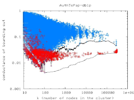
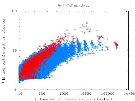
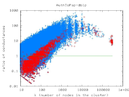
In light of this, let’s say that we are interested in finding reasonably good clusters of size $10^{3}$ or $10^{4}$ nodes in a large social or information network. (See [31] for why this might be interesting.) In that case, Figure 1 presents very typical results. Figure 1(a) presents a scatter plot of the size-resolved conductance of clusters found with a flow-based approximation algorithm (in red) and a spectral-based approximation algorithm (in blue).²⁶²⁶26Ignore the “size-resolved” aspect of these plots, since by assumption we are interested in clusters of roughly $10^{3}$ or $10^{4}$ nodes (but [27, 28] provides details on this); and don’t worry about the details of the flow-based and spectral-based procedures, except to say that there is a nontrivial theory-practice gap (again, [27, 28] provides details). In this plot, lower values on the Y-axis correspond to better values of the objective function; and thus the flow-based procedure is unambiguously better than the spectral procedure at finding good-conductance clusters. On the other hand, how useful these clusters are for downstream applications is also of interest. Since we are not explicitly performing any regularization, we do not have any explicit “niceness” function, but we can examine empirical niceness properties of the clusters found by the two approximation procedures. Figures 1(b) and 1(c) presents these results for two different niceness measures. Here, lower values on the Y-axis correspond to “nicer” clusters, and again we are interested in clusters with lower Y-axis values. Thus, in many cases, the spectral procedure is clearly better than the flow-based procedure at finding nice clusters with reasonably good conductance values.

Formalizations aside, this empirical tradeoff between solution quality and solution niceness is basically the defining feature of statistical regularization—except that we are observing it here as a function of two different approximation algorithms for the same intractable combinatorial objective function. That is, although we have not explicitly put any regularization term anywhere, the fact that these two different approximation algorithms essentially filter the data through different metric and geometric spaces leaves easily-observed empirical artifacts on the output of those approximation algorithms.²⁷²⁷27For other data—in particular, constant-degree expanders—the situation should be reversed. That is, theory clearly predicts that locally-biased flow-based algorithms [3] will have better niceness properties than locally-biased spectral-based algorithms [1]. Observing this empirically on real data is difficult since data that are sufficiently unstructured to be expanders, in the sense of having no good partitions, tend to have very substantial degree heterogeneity. One possible response to these empirical results is is to say that conductance is not the “right” objective function and that we should come up with some other objective to formalize our intuition;²⁸²⁸28Conductance probably is the combinatorial quantity that most closely captures the intuitive bi-criterial notion of what it means for a set of nodes to be a good “community,” but it is still very far from perfect on many real data. but of course that other objective function will likely be intractable, and thus we will have to approximate it with a different spectral-based or flow-based (or some other) procedure, in which case the same implicit regularization issues will arise [27, 28].

In many applications, one would like to identify locally-biased graph partitions, i.e., clusters in a data graph that are “near” a prespecified set of nodes. For example, in nearly every reasonably large social or information network, there do not exist large good-conductance clusters, but there are often smaller clusters that are meaningful to the domain scientist [2, 27, 28]; in other cases, one might have domain knowledge about certain nodes, and one might want to use that to find locally-biased clusters in a semi-supervised manner [33]; while in other cases, one might want to perform algorithmic primitives such as solving linear equations in time that is nearly linear in the size of the graph [39, 1, 15].

One general approach to problems of this sort is to modify the usual objective function and then show that the solution to the modified problem inherits some or all of the nice properties of the original objective. For example, a natural way to formalize the idea of a locally-biased version of the leading nontrivial eigenvector of $\mathcal{L}$ that can then be used in a locally-biased version of the graph partitioning problem is to modify Problem (3) with a locality constraint as follows.

		$\displaystyle\underset{x}{\text{minimize}}$		$\displaystyle x^{T}\mathcal{L}x$		(8)
		subject to		$\displaystyle x^{T}x=1,$
		$\displaystyle x^{T}D^{1/2}1=0$
		$\displaystyle(x^{T}D^{1/2}s)^{2}\geq\kappa,$

where $s$ is a vector representing the “seed set,” and where $\kappa$ is a locality parameter. This locally-biased version of the usual spectral graph partitioning problem was introduced in [33], where it was shown that solution inherits many of the nice properties of the solution to the usual global spectral partitioning problem. In particular, the exact solution can be found relatively-quickly by running a so-called Personalized PageRank computation; if one performs a sweep cut on this solution vector in order to obtain a locally-biased partition, then one obtains Cheeger-like quality-of-approximation guarantees on the resulting cluster; and if the seed set consists of a single node, then this is a relaxation of the following locally-biased graph partitioning problem: given as input a graph $G=(V,E)$, an input node $u$, and a positive integer $k$, find a set of nodes $S\subseteq V$ achieving

$$\phi(u,k,G)=\min_{S\subseteq V:u\in S,\mathrm{vol}(S)\leq k}\phi(S),$$

(9)

i.e., find the best conductance set of nodes of volume no greater than $k$ that contains the input node $v$ [33]. This “optimization-based approach” has the advantage that it is explicitly solving a well-defined objective function, and as such it is useful in many small-scale to medium-scale applications [33]. But this approach has the disadvantage, at least for Web-scale graphs, that the computation of the locally-biased eigenvector “touches” all of the nodes in the graph—and this is very expensive, especially when one wants to find small clusters.

An alternative more “operational approach” is to do the following: run some sort of procedure, the steps of which are similar to the steps of an algorithm that would solve the problem exactly; and then either use the output of that procedure in a downstream application in a manner similar to how the exact answer would have been used, or prove a theorem about that output that is similar to what can be proved for the exact answer. As an example of this approach, [39, 1, 15] take as input some seed nodes and a locality parameter and then run a diffusion-based procedure to return as output a “good” cluster that is “nearby” the seed nodes. In each of these cases, the procedure is similar to the usual procedure,²⁹²⁹29Namely, the three diffusion-based procedures that were described in Section 3.1: [39] performs truncated random walks; [1] approximates Personalized PageRank vectors; and [15] runs a modified heat kernel procedure. except that at each step of the algorithm various “small” quantities are truncated to zero (or simply maintained at zero), thereby minimizing the number of nodes that need to be touched at each step of the algorithm. For example, [39] sets to zero very small probabilities, and [1] uses the so-called push algorithm [24, 10] to concentrate computational effort on that part of the vector where most of the nonnegligible changes will take place.

The outputs of these strongly local spectral methods obtain Cheeger-like quality-of-approximation guarantees, and by design these procedures are extremely fast—the running time depends on the size of the output and is independent even of the number of nodes in the graph. Thus, an advantage of this approach is that it opens up the possibility of performing more sophisticated eigenvector-based analytics on Web-scale data matrices; and these methods have already proven crucial in characterizing the clustering and community structure of social and information networks with up to millions of nodes [2, 27, 28]. At present, though, this approach has the disadvantage that it is very difficult to use: the exact statement of the theoretical results is extremely complicated, thereby limiting its interpretability; it is extremely difficult to characterize and interpret for downstream applications what actually is being computed by these procedures, i.e., it is not clear what optimization problem these approximation algorithms are solving exactly; and counterintuitive things like a seed node not being part of “its own cluster” can easily happen. At root, the reason for these difficulties is that the truncation and zeroing-out steps implicitly regularize—but they are done based on computational considerations, and it is not known what are the implicit statistical side-effects of these design decisions.

The precise relationship between these two approaches has not, to my knowledge, been characterized. Informally, though, the truncating-to-zero provides a “bias” that is analogous to the early-stopping of iterative methods, such as those described in Section 3.1, and that has strong structural similarities with thresholding and truncation methods, as commonly used in $\ell_{1}$-regularization methods and optimization more generally [19]. For example, the update step of the push algorithm, as used in [1], is a form of stochastic gradient descent [20], a method particularly well-suited for large-scale environments due to its connections with regularization and boosting [11]; and the algorithm terminates after a small number of iterations when a truncated residual vector equals zero [20], in a manner similar to other truncated gradient methods [25].

Perhaps more immediately-relevant to database theory and practice as well as to implementing these ideas in large-scale statistical data analysis applications is simply to note that this operational and interactive approach to database algorithms is already being adopted in practice. For example, in addition to empirical work that uses these methods to characterize the clustering and community structure of large networks [2, 27, 28], the body of work that uses diffusion-based primitives in database environments includes an algorithm to estimate PageRank on graph streams [37], the approximation of PageRank on large-scale dynamically-evolving social networks [6], and a MapReduce algorithm for the approximation of Personalized PageRank vectors of all the nodes in a graph [5].

References

- [1] R. Andersen, F.R.K. Chung, and K. Lang. Local graph partitioning using PageRank vectors. In FOCS ’06: Proceedings of the 47th Annual IEEE Symposium on Foundations of Computer Science, pages 475–486, 2006.
- [2] R. Andersen and K. Lang. Communities from seed sets. In WWW ’06: Proceedings of the 15th International Conference on World Wide Web, pages 223–232, 2006.
- [3] R. Andersen and K. Lang. An algorithm for improving graph partitions. In SODA ’08: Proceedings of the 19th ACM-SIAM Symposium on Discrete algorithms, pages 651–660, 2008.
- [4] S. Arora, S. Rao, and U. Vazirani. Geometry, flows, and graph-partitioning algorithms. Communications of the ACM, 51(10):96–105, 2008.
- [5] B. Bahmani, K. Chakrabarti, and D. Xin. Fast personalized PageRank on MapReduce. In Proceedings of the 37th SIGMOD international conference on Management of data, pages 973–984, 2011.
- [6] B. Bahmani, A. Chowdhury, and A. Goel. Fast incremental and personalized pagerank. Proceedings of the VLDB Endowment, 4(3):173–184, 2010.
- [7] P. Berkhin. A survey on PageRank computing. Internet Mathematics, 2(1):73–120, 2005.
- [8] P. Bickel and B. Li. Regularization in statistics. TEST, 15(2):271–344, 2006.
- [9] L. Blum, F. Cucker, M. Shub, and S. Smale. Complexity and real computation: A manifesto. International Journal of Bifurcation and Chaos, 6(1):3–26, 1996.
- [10] P. Boldi and S. Vigna. The push algorithm for spectral ranking. Technical report. Preprint: arXiv:1109.4680 (2011).
- [11] L. Bottou. Large-scale machine learning with stochastic gradient descent. In Proceedings of the 19th International Conference on Computational Statistics (COMPSTAT’2010), pages 177–187, 2010.
- [12] J. Cheeger. A lower bound for the smallest eigenvalue of the Laplacian. In Problems in Analysis, Papers dedicated to Salomon Bochner, pages 195–199. Princeton University Press, 1969.
- [13] Z. Chen and S. Haykin. On different facets of regularization theory. Neural Computation, 14(12):2791–2846, 2002.
- [14] F.R.K. Chung. Spectral graph theory, volume 92 of CBMS Regional Conference Series in Mathematics. American Mathematical Society, 1997.
- [15] F.R.K. Chung. The heat kernel as the pagerank of a graph. Proceedings of the National Academy of Sciences of the United States of America, 104(50):19735–19740, 2007.
- [16] J. Cohen, B. Dolan, M. Dunlap, J. M. Hellerstein, and C. Welton. MAD skills: new analysis practices for big data. Proceedings of the VLDB Endowment, 2(2):1481–1492, 2009.
- [17] J. Dean and S. Ghemawat. MapReduce: Simplified data processing on large clusters. In Proceedings of the 6th conference on Symposium on Operating Systems Design and Implementation, pages 10–10, 2004.
- [18] R. Agrawal et al. The Claremont report on database research. ACM SIGMOD Record, 37(3):9–19, 2008.
- [19] J. Friedman, T. Hastie, and R. Tibshirani. Additive logistic regression: a statistical view of boosting. Annals of Statistics, 28(2):337–407, 2000.
- [20] D.F. Gleich and M.W. Mahoney. Unpublished results, 2012.
- [21] S. Guattery and G.L. Miller. On the quality of spectral separators. SIAM Journal on Matrix Analysis and Applications, 19:701–719, 1998.
- [22] T. Hastie, R. Tibshirani, and J. Friedman. The Elements of Statistical Learning. Springer-Verlag, New York, 2003.
- [23] S. Hoory, N. Linial, and A. Wigderson. Expander graphs and their applications. Bulletin of the American Mathematical Society, 43:439–561, 2006.
- [24] G. Jeh and J. Widom. Scaling personalized web search. In WWW ’03: Proceedings of the 12th International Conference on World Wide Web, pages 271–279, 2003.
- [25] J. Langford, L. Li, and T. Zhang. Sparse online learning via truncated gradient. Journal of Machine Learning Research, 10:777–801, 2009.
- [26] T. Leighton and S. Rao. Multicommodity max-flow min-cut theorems and their use in designing approximation algorithms. Journal of the ACM, 46(6):787–832, 1999.
- [27] J. Leskovec, K.J. Lang, A. Dasgupta, and M.W. Mahoney. Statistical properties of community structure in large social and information networks. In WWW ’08: Proceedings of the 17th International Conference on World Wide Web, pages 695–704, 2008.
- [28] J. Leskovec, K.J. Lang, and M.W. Mahoney. Empirical comparison of algorithms for network community detection. In WWW ’10: Proceedings of the 19th International Conference on World Wide Web, pages 631–640, 2010.
- [29] N. Linial, E. London, and Y. Rabinovich. The geometry of graphs and some of its algorithmic applications. Combinatorica, 15(2):215–245, 1995.
- [30] M. W. Mahoney. Randomized algorithms for matrices and data. Foundations and Trends in Machine Learning. NOW Publishers, Boston, 2011. Also available at: arXiv:1104.5557.
- [31] M. W. Mahoney. Algorithmic and statistical perspectives on large-scale data analysis. In U. Naumann and O. Schenk, editors, Combinatorial Scientific Computing, Chapman & Hall/CRC Computational Science. CRC Press, 2012.
- [32] M. W. Mahoney and L. Orecchia. Implementing regularization implicitly via approximate eigenvector computation. In Proceedings of the 28th International Conference on Machine Learning, pages 121–128, 2011.
- [33] M. W. Mahoney, L. Orecchia, and N. K. Vishnoi. A local spectral method for graphs: with applications to improving graph partitions and exploring data graphs locally. Technical report. Preprint: arXiv:0912.0681 (2009).
- [34] A. Neumaier. Solving ill-conditioned and singular linear systems: A tutorial on regularization. SIAM Review, 40:636–666, 1998.
- [35] L. Page, S. Brin, R. Motwani, and T. Winograd. The PageRank citation ranking: Bringing order to the web. Technical report, Stanford InfoLab, 1999.
- [36] P. O. Perry and M. W. Mahoney. Regularized Laplacian estimation and fast eigenvector approximation. In Annual Advances in Neural Information Processing Systems 25: Proceedings of the 2011 Conference, 2011.
- [37] A. Das Sarma, S. Gollapudi, and R. Panigrahy. Estimating PageRank on graph streams. In Proceedings of the 27th ACM Symposium on Principles of Database Systems, pages 69–78, 2008.
- [38] S. Smale. Some remarks on the foundations of numerical analysis. SIAM Review, 32(2):211–220, 1990.
- [39] D.A. Spielman and S.-H. Teng. Nearly-linear time algorithms for graph partitioning, graph sparsification, and solving linear systems. In STOC ’04: Proceedings of the 36th annual ACM Symposium on Theory of Computing, pages 81–90, 2004.
- [40] A.N. Tikhonov and V.Y. Arsenin. Solutions of Ill-Posed Problems. W.H. Winston, Washington, D.C., 1977.
- [41] V.V. Vazirani. Approximation Algorithms. Springer-Verlag, New York, 2001.
- [42] S. Vigna. Spectral ranking. Technical report. Preprint: arXiv:0912.0238 (2009).