This paper was converted on www.awesomepapers.org from LaTeX by an anonymous user.
Want to know more? Visit the Converter page.

Approximating arrival costs in distributed moving horizon estimation: A recursive method

Xiaojie Lia, Xunyuan Yina,b,

aSchool of Chemistry, Chemical Engineering and Biotechnology, Nanyang Technological University,

62 Nanyang Drive, 637459, Singapore

bEnvironmental Process Modelling Centre, Nanyang Environment and Water Research Institute (NEWRI),

Nanyang Technological University, 1 CleanTech Loop, 637141, Singapore
Corresponding author: Xunyuan Yin. Tel: (+65)63168746. Email: xunyuan.yin@ntu.edu.sg
Abstract

In this paper, we present a new approach to distributed moving horizon estimation for constrained nonlinear processes. The method involves approximating the arrival costs of local estimators through a recursive framework. First, distributed full-information estimation for linear unconstrained systems is presented, which serves as the foundation for deriving the analytical expression of the arrival costs for the local estimators. Subsequently, we develop a recursive arrival cost design for linear distributed moving horizon estimation. Sufficient conditions are derived to ensure the stability of the estimation error for constrained linear systems. Next, we extend the arrival cost design derived for linear systems to account for nonlinear systems, and a partition-based constrained distributed moving horizon estimation algorithm for nonlinear systems is formulated. A benchmark chemical process is used to illustrate the effectiveness and superiority of the proposed method.

Keywords: Distributed state estimation, moving horizon estimation, arrival cost approximation, nonlinear processes

1 Introduction

The partition-based distributed framework has emerged as a promising structure for developing scalable and flexible decision-making solutions for large-scale complex industrial processes, since it can provide higher fault tolerance, reduced computational complexity, and increased flexibility for system maintenance [1, 2, 3]. Within a partition-based distributed decision-making framework, a large-scale process is partitioned into smaller subsystems that are interconnected with each other. Multiple decision-making units are deployed for the subsystems and coordinate their decisions through real-time communication [4, 5, 6]. To enable distributed decision-making systems to take informed control actions for appropriate process operation, it is crucial to have distributed state estimation capabilities that can provide real-time full-state estimates for the underlying systems [2, 7, 8]. In this paper, we focus on partition-based distributed state estimation for general nonlinear systems.

As an effective distributed state estimation approach, distributed moving horizon estimation (DMHE) offers the capability to handle process nonlinearity and address constraints imposed on both state variables and process disturbances [7, 8, 9, 10, 11, 12, 13, 14, 15, 16]. In [7], non-iterative partition-based DMHE algorithms were proposed for linear systems considering constraints on state variables and process disturbances. These algorithms design local estimators based on partitioned subsystem models, with each local estimator handling state estimation for the corresponding subsystem with non-overlapping states. In [8, 9, 10, 11, 12], partition-based DMHE approaches that require iterative executions within each sampling period were proposed for linear systems; these designs ensure the convergence of the state estimates generated by DMHE to their the corresponding centralized moving horizon estimation (MHE) counterparts. Based on these approaches, the objective function of centralized MHE is partitioned into several individual objective functions. An additional term is then incorporated with each partitioned objective function to construct the local objective function for the proposed DMHE algorithms. Particularly, in [8, 9, 10], a sensitivity term is integrated with the partitioned objective function to account for the impact of each local decision variable on the objective functions of interconnected subsystems, while in [11, 12], penalties on measurement noise from interconnected subsystems are incorporated to form the local objective function of each estimator. In [13, 14], partition-based DMHE approaches for nonlinear systems were proposed. In [15, 16], DMHE for constrained nonlinear systems was addressed in a way that an auxiliary observer is integrated with the corresponding MHE to form an enhanced MHE-based constrained estimator for each subsystem of the entire nonlinear process.

In MHE design, previous information not included in the current estimation window can be summarized by a function referred to as arrival cost. An accurate approximation of the arrival cost can enhance estimation performance [17, 18]. Additionally, a well-approximated arrival cost allows for a reduction in the length of the estimation window without compromising the accuracy of state estimates [18]. This reduction in the estimation window length can enhance the computational efficiency by decreasing the complexity of the optimization problem. In centralized MHE designs, various methods have been proposed to approximate the arrival cost. For linear systems, the Kalman filter has been widely used in the approximation of arrival cost [19, 20]. For nonlinear systems, solutions for approximating the arrival cost of centralized MHE include extended Kalman filter [21, 22], unscented Kalman filter [17], and particle filter [18]. In a distributed context, accurately approximating the arrival costs for the local estimators of DMHE becomes a more complicated problem. Different approximation methods for arrival cost approximation have been adopted for linear DMHE. In [8, 9, 10, 11, 12], the arrival cost was formulated as a weighted squared error between the state estimate and the a priori prediction, weighted by a constant matrix, which is fine-tuned to satisfy stability conditions. Additionally, in [7], a Kalman filter design for an auxiliary system was leveraged to approximate the weighting matrix for the arrival cost at each sampling instant. In [23], a partition-based DMHE method was proposed for the state estimation of data-driven subsystem models. In this work, the update of the arrival cost for DMHE design was facilitated by using a partition-based distributed Kalman filter approach proposed in [24]. Meanwhile, results on approximating the arrival costs for nonlinear DMHE algorithms have been limited. In [13] where a two-time-scale nonlinear DMHE was proposed, the arrival costs for the local estimators were not considered. In [14], the weighting matrix for the arrival cost design of each estimator was updated at each sampling instant. However, this paper only presents the conditions for the weighting matrix to satisfy and does not explicitly provide the update formula for the weighting matrix. In [15, 16], decentralized extended Kalman filters were utilized to approximate the arrival costs for local estimators of observer-enhanced DMHE. However, in each of the two designs, the interactive dynamics were not taken into account.

In this paper, we address the problem of approximating the arrival costs for the local estimators of a partition-based DMHE design and formulate a partition-based distributed estimation scheme for general nonlinear processes with state constraints. The objective of this work is achieved in four steps: 1) we derive an analytical expression of the arrival cost for each local estimator of the DMHE in the unconstrained linear context from the design of the distributed full-information estimation formulation in [24]; 2) we conduct the stability analysis for the proposed DMHE algorithm for linear systems with state constraints; 3) the analytical expression of arrival cost obtained for linear unconstrained systems is extended to account for nonlinear systems; 4) we formulate a partition-based constrained DMHE algorithm for general nonlinear systems, where each local estimator incorporates output measurements of the interacting subsystems and approximates the local arrival cost using the derived recursive solution. The effectiveness of the proposed method is demonstrated using a simulated chemical process. Some initial findings from this study were presented in a conference paper [25]. Compared with [25], this paper presents the stability analysis for the proposed DMHE algorithm for linear systems with state constraints. Additionally, we include additional comparisons to demonstrate the efficacy and superiority of the proposed DMHE approach.

2 Preliminaries

2.1 Notation

diag{A1,,An}\text{diag}\left\{A_{1},\ldots,A_{n}\right\} represents the block diagonal matrix with blocks AiA_{i}, i=1,,ni=1,\ldots,n. [Aij][A_{ij}] represents a block matrix where the AijA_{ij} is the submatrix in the iith row and the jjth column. InI_{n} is an n×nn\times n identity matrix. zA2=zTAz\|z\|_{A}^{2}=z^{\mathrm{T}}Az is the square of the weighted Euclidean norm of vector zz. col{z1,,zn}\text{col}\{z_{1},\ldots,z_{n}\} denotes a column vector containing a sequence z1,,znz_{1},\ldots,z_{n}. {z}ab=col{za,za+1,,zb}\{z\}_{a}^{b}=\text{col}\{z_{a},z_{a+1},\ldots,z_{b}\}.

2.2 System description

Let us consider nonlinear systems consisting of nn interconnected subsystems. The dynamics of the iith subsystem, i𝕀={1,2,,n}i\in\mathbb{I}=\{1,2,\ldots,n\}, are expressed as follows:

xk+1i\displaystyle x^{i}_{k+1} =fi(xki,Xki)+wki\displaystyle=f_{i}\big{(}x^{i}_{k},X^{i}_{k}\big{)}+w^{i}_{k} (1a)
yki\displaystyle y^{i}_{k} =hi(xki)+vki\displaystyle=h_{i}(x^{i}_{k})+v^{i}_{k} (1b)

where kk denotes discrete-sampling instant; xkinxix^{i}_{k}\in\mathbb{R}^{n_{x^{i}}} and ykinyiy^{i}_{k}\in\mathbb{R}^{n_{y^{i}}} represent the state vector and output measurements of the iith subsystem, respectively; XkinXiX^{i}_{k}\in\mathbb{R}^{n_{X^{i}}} is a vector of the states of all the subsystems that have direct influence on the dynamics of subsystem ii; wkinxiw^{i}_{k}\in\mathbb{R}^{n_{x^{i}}} and vkinyiv^{i}_{k}\in\mathbb{R}^{n_{y^{i}}} represent the unknown process disturbances and measurement noise associated with subsystem ii, respectively; fif_{i} is a vector-value nonlinear function characterizing the dynamics of subsystem ii; hih_{i} is the output measurement function for subsystem ii, i𝕀i\in\mathbb{I}.

By considering the variables for the entire system as the aggregation of the variables for each subsystem ii, i𝕀i\in\mathbb{I}: zk=col{zk1,,zkn}nzz_{k}={\rm{col}}\{z^{1}_{k},\ldots,z^{n}_{k}\}\in\mathbb{R}^{n_{z}} for vector z{x,y,w,v}z\in\{x,y,w,v\}, the dynamics of the entire system can be formulated in the following compact form:

xk+1\displaystyle x_{k+1} =f(xk)+wk\displaystyle=f(x_{k})+w_{k} (2a)
yk\displaystyle y_{k} =h(xk)+vk\displaystyle=h(x_{k})+v_{k} (2b)

where f(xk)f(x_{k}) and h(xk)h(x_{k}) can be obtained from fi(xk,Xki)f_{i}(x_{k},X^{i}_{k}) and hi(xki)h_{i}(x^{i}_{k}), respectively.

2.3 Problem formulation

In this work, we aim to propose a partition-based DMHE algorithm for nonlinear systems, which integrates a recursive update mechanism for the arrival cost of each local estimator of the distributed scheme. To achieve this goal, we first present a distributed full-information estimation (FIE) design by partitioning the objective function of a centralized FIE problem. From this design, we derive the analytical expression of the arrival cost for the proposed DMHE method in a linear context. Subsequently, we formulate the proposed DMHE method based on the obtained arrival costs, and sufficient conditions are provided to guarantee the stability of the proposed DMHE approach under state constraints. Finally, the obtained arrival costs for linear systems are extended to account for the nonlinear systems, and a partition-based DMHE algorithm for constrained nonlinear context is formulated.

Based on the above consideration, first, we start by examining a class of linear systems consisting of nn subsystems. The dynamics of iith linear subsystem, i𝕀i\in\mathbb{I}, are described as follows:

xk+1i\displaystyle x^{i}_{k+1} =Aiixki+l𝕀{i}Ailxkl+wki\displaystyle=A_{ii}x^{i}_{k}+\sum_{l\in\mathbb{I}\setminus\{i\}}A_{il}x^{l}_{k}+w^{i}_{k} (3a)
yki\displaystyle y^{i}_{k} =Ciixki+vki\displaystyle=C_{ii}x^{i}_{k}+v^{i}_{k} (3b)

where AiiA_{ii}, AilA_{il}, and CiiC_{ii}, i𝕀i\in\mathbb{I}, l𝕀{i}l\in\mathbb{I}\setminus\{i\}, are subsystem matrices of compatible dimensions.

Based on the linear subsystem models in (3), we will design MHE-based local estimators. These estimators will then be integrated to formulate a linear DMHE design, which will be extended to account for state estimation of nonlinear systems in (1). A compact form of the linear system comprising all the subsystems in the form of (3) is described as follows:

xk+1\displaystyle x_{k+1} =Axk+wk\displaystyle=Ax_{k}+w_{k} (4a)
yk\displaystyle y_{k} =Cxk+vk\displaystyle=Cx_{k}+v_{k} (4b)

where A=[Ail]A=[A_{il}] represents a block matrix where AilA_{il} is the submatrix in the iith row and the llth column; C=diag{C11,,Cnn}C=\mathrm{diag}\{C_{11},\ldots,C_{nn}\}.

2.4 Centralized full-information estimation

Full-information estimation (FIE) is an optimization-based state estimation approach, which can be viewed as a least-squares estimation method that minimizes the cumulative sum of squared errors from the initial time instant to the current time instant. Specifically, at each sampling instant kk, based on the linear model in (4), a centralized FIE design can be formulated as follows [26]:

min{x^j}j=0j=kΦ¯k=j=0k1w^jQ12+j=0kv^jR12+x^0x¯0P012\displaystyle\min_{\{\hat{x}_{j}\}_{j=0}^{j=k}}\bar{\Phi}_{k}=\sum_{j=0}^{k-1}\|\hat{w}_{j}\|^{2}_{Q^{-1}}+\sum_{j=0}^{k}\|\hat{v}_{j}\|^{2}_{R^{-1}}+\|\hat{x}_{0}-\bar{x}_{0}\|_{P_{0}^{-1}}^{2}
s.t.x^j+1=Ax^j+w^j\displaystyle\quad\text{s.t.}~{}~{}~{}~{}~{}\hat{x}_{j+1}=A\hat{x}_{j}+\hat{w}_{j} (5a)
yj=Cx^j+v^j\displaystyle\quad\quad\quad~{}~{}~{}~{}~{}~{}\,y_{j}=C\hat{x}_{j}+\hat{v}_{j} (5b)

where x^j\hat{x}_{j} is an estimate of state xjx_{j}; x¯0\bar{x}_{0} is an a priori estimate of initial state x0x_{0}; w^j\hat{w}_{j} and v^j\hat{v}_{j} are estimates of process disturbances wjw_{j} and measurement noise vjv_{j}, respectively; P0P_{0}, QQ, and RR are positive-definite weighting matrices. It is noted that as the number of sampling instants increases over time, the associated optimization problem in (5) becomes increasingly complex and intractable. FIE is important for the design and analysis of the MHE approaches [26, 27]. In the next section, we introduce a distributed FIE design, which is used to guide the development of the DMHE approach.

3 Distributed full-information estimation

In this section, a distributed FIE problem is formulated based on the linear subsystem models in (3). First, we partition the global objective function of the centralized FIE design in (5), following [24]. Subsequently, each partitioned objective function is integrated with the sensor measurements from interconnected subsystems to construct the local objective function of each local estimator.

3.1 Construction of local objective functions

Following [24], the global objective function of the centralized FIE algorithm Φ¯k\bar{\Phi}_{k} is decomposed into Φ¯ki\bar{\Phi}^{i}_{k}, i𝕀i\in\mathbb{I}, such that Φ¯k=i𝕀Φ¯ki\bar{\Phi}_{k}=\sum_{i\in\mathbb{I}}\bar{\Phi}^{i}_{k}. The objective function of each local estimator is described as follows:

Φ¯ki\displaystyle\bar{\Phi}^{i}_{k} =j=0k1w^jiQi12+j=0kv^jiRi12+x^0ix¯0iPi,012\displaystyle=\sum_{j=0}^{k-1}\|\hat{w}^{i}_{j}\|^{2}_{Q_{i}^{-1}}+\sum_{j=0}^{k}\|\hat{v}^{i}_{j}\|^{2}_{R_{i}^{-1}}+\|\hat{x}^{i}_{0}-\bar{x}^{i}_{0}\|_{P_{i,0}^{-1}}^{2} (6)

where x^0i\hat{x}^{i}_{0} is an estimate of the iith subsystem state x0ix^{i}_{0}; x¯0i\bar{x}^{i}_{0} is an initial guess of x0ix^{i}_{0}; w^ji\hat{w}^{i}_{j} and v^ji\hat{v}^{i}_{j} are the estimates of disturbances wjiw^{i}_{j} and measurement noise vjiv^{i}_{j} of the iith subsystem, respectively. It is noted that the sensor measurements from the interconnected subsystems can provide valuable information for estimating the local subsystem states. Inspired by the objective function designs for the distributed state estimation algorithms proposed in [8, 10, 24], each local objective function of the local estimator of distributed FIE is presented as follows:

Φki\displaystyle\Phi_{k}^{i} =Φ¯ki+l𝕀{i}j=0kv^jlRl12\displaystyle=\bar{\Phi}_{k}^{i}+\sum_{l\in\mathbb{I}\setminus\{i\}}\sum_{j=0}^{k}\|\hat{v}_{j}^{l}\|^{2}_{R_{l}^{-1}}
=j=0k1w^jiQi12+j=0kv^j[i]R12+x^0ix¯0iPi,012\displaystyle=\sum_{j=0}^{k-1}\|\hat{w}^{i}_{j}\|^{2}_{Q_{i}^{-1}}+\sum_{j=0}^{k}\|\hat{v}^{[i]}_{j}\|^{2}_{R^{-1}}+\|\hat{x}^{i}_{0}-\bar{x}^{i}_{0}\|_{P_{i,0}^{-1}}^{2} (7)

where v^j[i]\hat{v}^{[i]}_{j} is an estimate of measurement noise vjv_{j} of the entire system within estimator ii; Pi,0P_{i,0}, QiQ_{i}, and RiR_{i} are the iith diagonal block of weighting matrices P0P_{0}, QQ, and RR, respectively. The key difference between Φ¯ki\bar{\Phi}_{k}^{i} in (6) and Φki\Phi_{k}^{i} in (3.1) is that Φki\Phi_{k}^{i} includes additional information on the sensor measurements of interconnected subsystems, which can provide valuable insights for the reconstruction of the local subsystem states.

3.2 Distributed full-information estimation formulation

At sampling instant kk, the local estimator for the iith subsystem of distributed FIE can be formulated by leveraging the local objective function proposed in (3.1):

min{x^ji}j=0j=kΦki=j=0k1w^jiQi12+j=0kv^j[i]R12+x^0ix¯0iPi,012\displaystyle\min_{\{\hat{x}^{i}_{j}\}_{j=0}^{j=k}}\Phi^{i}_{k}=\sum_{j=0}^{k-1}\|\hat{w}^{i}_{j}\|^{2}_{Q_{i}^{-1}}+\sum_{j=0}^{k}\|\hat{v}^{[i]}_{j}\|^{2}_{R^{-1}}+\|\hat{x}^{i}_{0}-\bar{x}^{i}_{0}\|_{P_{i,0}^{-1}}^{2}
s.t.x^j+1i=Aiix^ji+l𝕀{i}Ailx~jl+w^ji\displaystyle~{}\,\mathrm{s.t.}~{}\hat{x}_{j+1}^{i}=A_{ii}\hat{x}_{j}^{i}+\sum_{l\in\mathbb{I}\setminus\{i\}}A_{il}\tilde{x}_{j}^{l}+\hat{w}_{j}^{i} (8a)
y0=C[:,i]x^0i+l𝕀{i}C[:,l]x~0l+v^0[i]\displaystyle~{}\,\quad~{}~{}\quad\,y_{0}=C_{[:,i]}\hat{x}_{0}^{i}+\sum_{l\in\mathbb{I}\setminus\{i\}}C_{[:,l]}\tilde{x}_{0}^{l}+\hat{v}_{0}^{[i]} (8b)
yj+1=C(A[:,i]x^ji+l𝕀{i}A[:,l]x~jl)+vj+1[i],j=0,,k1\displaystyle~{}\,\quad~{}~{}~{}y_{j+1}=C(A_{[:,i]}\hat{x}_{j}^{i}+\sum_{l\in\mathbb{I}\setminus\{i\}}A_{[:,l]}\tilde{x}_{j}^{l})+v_{j+1}^{[i]},~{}j=0,\ldots,k-1 (8c)

where A[:,i]A_{[:,i]} and C[:,i]C_{[:,i]} comprise the columns of AA and CC with respect to the state of xix^{i}, respectively; x~jl\tilde{x}_{j}^{l} is a (conservative) state estimate of subsystem ll for sampling instant jj made available to the estimator of subsystem ii, which is determined as:

x~jl={x^j|k1l,forj=1,,k1x¯0l,forj=0\normalsize\tilde{x}_{j}^{l}=\left\{\begin{array}[]{l}\hat{x}_{j|k-1}^{l},~{}~{}~{}~{}~{}{\text{for}}~{}j=1,\ldots,k-1{}{}\\[3.00003pt] \bar{x}_{0}^{l},~{}~{}~{}~{}~{}~{}~{}~{}~{}~{}{\text{for}}~{}j=0{}{}\end{array}\right. (9)

In (9), x^j|k1l\hat{x}_{j|k-1}^{l} is the state estimate of xjlx^{l}_{j} calculated by the llth estimator at sampling instant k1k-1, and x¯0l\bar{x}_{0}^{l} denotes an initial guess of x0lx_{0}^{l}, l𝕀{i}l\in\mathbb{I}\setminus\{i\}. We utilize the state estimates x^j|k1l\hat{x}_{j|k-1}^{l} obtained at the previous time instant k1k-1 because they are calculated based on the most recent available sensor measurements. In the remainder of this paper, we simplify the subscript by omitting “|k|k”, and we denote x^j|ki\hat{x}_{j|k}^{i} by x^ji\hat{x}_{j}^{i} for brevity.

4 Distributed moving horizon estimation for linear systems

In this section, a linear DMHE design with a recursive update of arrival costs for the local estimators is presented. The stability of the proposed linear DMHE design is analyzed. First, we obtain an analytical recursive expression of the arrival cost by leveraging the distributed FIE in (8). Following this, we formulate a DMHE design where the arrival cost of each local estimator is updated using the derived recursive method for linear systems with state constraints. Additionally, we prove the stability of the proposed DMHE approach.

Inspired by the DMHE designs proposed by [8] and [12], the iith estimator of the proposed DMHE at sampling instant kk solves the optimization below:

min{x^ji}j=kNkΦki,MHEsubject to (8a), (8b), and (8c)\min_{\{\hat{x}_{j}^{i}\}_{j=k-N}^{k}}\Phi_{k}^{i,\mathrm{MHE}}~{}\text{subject to \eqref{eq:upd0_2}, \eqref{eq:upd0_4}, and \eqref{eq:upd0_3}} (10a)
with
Φki,MHE\displaystyle\Phi_{k}^{i,\mathrm{MHE}} =VkNi,o+j=kNk1w^jiQi12+j=kNkv^j[i]R12\displaystyle=V_{k-N}^{i,o}+\sum_{j=k-N}^{k-1}\|\hat{w}^{i}_{j}\|^{2}_{Q_{i}^{-1}}+\sum_{j=k-N}^{k}\|\hat{v}_{j}^{[i]}\|^{2}_{R^{-1}} (10b)

where N1N\geq 1 is the length of the estimation window; VkNi,oV_{k-N}^{i,o} is the arrival cost that summarizes the historical information excluded from the estimation window. The detailed arrival cost design will be discussed in Section 4.1. Before proceeding, we introduce two lemmas, which will be used to derive the expression of the arrival cost for each estimator of the proposed DMHE design.

Lemma 1.

([28]) Consider the following two quadratic functions:

J1(x)=xaA12,J2(x)=CxbB12,J_{1}(x)=\|x-a\|_{A^{-1}}^{2},\quad J_{2}(x)=\|Cx-b\|_{B^{-1}}^{2},

where AA and BB are positive definite matrices; a and b are two vectors of compatible dimensions. Then, it holds that

J1(x)+J2(x)=xσH12+π,J_{1}(x)+J_{2}(x)=\|x-\sigma\|_{H^{-1}}^{2}+\pi,

where

H\displaystyle H =AACT(CACT+B)1CA,\displaystyle=A-AC^{\mathrm{T}}(CAC^{\mathrm{T}}+B)^{-1}CA,
σ\displaystyle\sigma =a+ACT(CACT+B)1(bCa),\displaystyle=a+AC^{\mathrm{T}}(CAC^{\mathrm{T}}+B)^{-1}(b-Ca),
π\displaystyle\pi =J1(σ)+J2(σ).\displaystyle=J_{1}(\sigma)+J_{2}(\sigma).

Lemma 2.

(Woodbury matrix identity [29]) If matrices AA and DD have full rank, then the following equations hold:

(A+BDC)1\displaystyle(A+BDC)^{-1} =A1A1B(CA1B+D1)1CA1\displaystyle=A^{-1}-A^{-1}B(CA^{-1}B+D^{-1})^{-1}CA^{-1}
(A+BDC)1BD\displaystyle(A+BDC)^{-1}BD =A1B(D1+CA1B)1\displaystyle=A^{-1}B(D^{-1}+CA^{-1}B)^{-1}

4.1 Arrival costs for linear systems

By comparing the design of the distributed FIE in (8) with the proposed DMHE in (10), the arrival cost VkNi,oV_{k-N}^{i,o} can be constructed by deriving the analytical solution to the following optimization problem:

VkNi,o=min{x^ji}j=0kN1VkNisubject to (8a), (8b), and (8c)V_{k-N}^{i,o}=\min_{\{\hat{x}_{j}^{i}\}_{j=0}^{k-N-1}}V_{k-N}^{i}~{}\text{subject to \eqref{eq:upd0_2}, \eqref{eq:upd0_4}, and \eqref{eq:upd0_3}}

where

VkNi\displaystyle V_{k-N}^{i} =x^0ix¯0iPi,012+j=0kN1w^jiQi12+j=0kN1v^j[i]R12\displaystyle=\|\hat{x}_{0}^{i}-\bar{x}_{0}^{i}\|^{2}_{P_{i,0}^{-1}}+\sum_{j=0}^{k-N-1}\|\hat{w}^{i}_{j}\|^{2}_{Q_{i}^{-1}}+\sum_{j=0}^{k-N-1}\|\hat{v}_{j}^{[i]}\|^{2}_{R^{-1}}

First, we consider the arrival cost V1i,oV_{1}^{i,o}, which can be formulated by deriving the analytical solution to the optimization problem below:

V1i,o=minx^0iV1isubject to (8a) and (8b) forj=0V_{1}^{i,o}=\min_{\hat{x}_{0}^{i}}V_{1}^{i}~{}\text{subject to \eqref{eq:upd0_2} and \eqref{eq:upd0_4} for}~{}j=0 (11a)
where
V1i\displaystyle V_{1}^{i} =x^0ix¯0iPi,012+v^0[i]R12+w^0iQi12\displaystyle=\|\hat{x}_{0}^{i}-\bar{x}_{0}^{i}\|^{2}_{P_{i,0}^{-1}}+\|\hat{v}_{0}^{[i]}\|^{2}_{R^{-1}}+\|\hat{w}_{0}^{i}\|^{2}_{Q_{i}^{-1}} (11b)

Considering (8b) and Lemma 1, V1iV_{1}^{i} can be rewritten as

V1i\displaystyle V^{i}_{1} =x^0ix¯0iPi,012+y0C[:,i]x^0il𝕀{i}C[:,l]x~0lR12+w^0iQi12\displaystyle=\|\hat{x}_{0}^{i}-\bar{x}_{0}^{i}\|^{2}_{P_{i,0}^{-1}}+\|y_{0}-C_{[:,i]}\hat{x}_{0}^{i}-\sum_{l\in\mathbb{I}\setminus\{i\}}C_{[:,l]}\tilde{x}_{0}^{l}\|^{2}_{R^{-1}}+\|\hat{w}_{0}^{i}\|^{2}_{Q_{i}^{-1}}
=x^0ix˘0iP˘i,012+π0i+w^0iQi12\displaystyle=\|\hat{x}_{0}^{i}-\breve{x}_{0}^{i}\|^{2}_{\breve{P}_{i,0}^{-1}}+\pi^{i}_{0}+\|\hat{w}_{0}^{i}\|^{2}_{Q_{i}^{-1}} (12)

where

P˘i,0\displaystyle\breve{P}_{i,0} =Pi,0Pi,0C[:,i]T(C[:,i]Pi,0C[:,i]T+R)1C[:,i]Pi,0\displaystyle=P_{i,0}-P_{i,0}C_{[:,i]}^{\mathrm{T}}(C_{[:,i]}P_{i,0}C_{[:,i]}^{\mathrm{T}}+R)^{-1}C_{[:,i]}P_{i,0}
x˘0i\displaystyle\breve{x}_{0}^{i} =x¯0i+Pi,0C[:,i]T(C[:,i]Pi,0C[:,i]T+R)1(y0C[:,i]x¯0il𝕀{i}C[:,l]x~0l)\displaystyle=\bar{x}_{0}^{i}+P_{i,0}C_{[:,i]}^{\mathrm{T}}(C_{[:,i]}P_{i,0}C_{[:,i]}^{\mathrm{T}}+R)^{-1}(y_{0}-C_{[:,i]}\bar{x}_{0}^{i}-\sum_{l\in\mathbb{I}\setminus\{i\}}C_{[:,l]}\tilde{x}_{0}^{l})
π0i\displaystyle\pi^{i}_{0} =x˘0ix¯0iPi,012+y0C[:,i]x˘0il𝕀{i}C[:,l]x~0lR12\displaystyle=\|\breve{x}_{0}^{i}-\bar{x}_{0}^{i}\|^{2}_{P_{i,0}^{-1}}+\|y_{0}-C_{[:,i]}\breve{x}_{0}^{i}-\sum_{l\in\mathbb{I}\setminus\{i\}}C_{[:,l]}\tilde{x}_{0}^{l}\|^{2}_{R^{-1}}

As π0i\pi^{i}_{0} is a constant, we do not need to take it into account when solving the optimization problem (11). According to (8a), Lemma 1, and Lemma 2, it is further obtained that

V1i\displaystyle V^{i}_{1} =x^0ix˘0iP˘i,012+x^1iAiix^0il𝕀{i}Ailx~0lQi12\displaystyle=\|\hat{x}_{0}^{i}-\breve{x}_{0}^{i}\|^{2}_{\breve{P}_{i,0}^{-1}}+\|\hat{x}_{1}^{i}-A_{ii}\hat{x}_{0}^{i}-\sum_{l\in\mathbb{I}\setminus\{i\}}A_{il}\tilde{x}_{0}^{l}\|^{2}_{Q_{i}^{-1}}
=x^0iσ˘0iH0i2+π˘0i\displaystyle=\|\hat{x}_{0}^{i}-\breve{\sigma}^{i}_{0}\|^{2}_{H_{0}^{i}}+\breve{\pi}^{i}_{0} (13)

where

H0i\displaystyle H_{0}^{i} =P˘i,01+AiiTQi1Aii\displaystyle=\breve{P}_{i,0}^{-1}+A_{ii}^{\mathrm{T}}Q_{i}^{-1}A_{ii} (14a)
σ˘0i\displaystyle\breve{\sigma}^{i}_{0} =x˘0i+P˘i,0AiiT(AiiP˘i,0AiiT+Qi)1(x^1iAiix˘0il𝕀{i}Ailx~0l)\displaystyle=\breve{x}_{0}^{i}+\breve{P}_{i,0}A_{ii}^{\mathrm{T}}(A_{ii}\breve{P}_{i,0}A_{ii}^{\mathrm{T}}+Q_{i})^{-1}(\hat{x}_{1}^{i}-A_{ii}\breve{x}_{0}^{i}-\sum_{l\in\mathbb{I}\setminus\{i\}}A_{il}\tilde{x}_{0}^{l}) (14b)
π˘0i\displaystyle\breve{\pi}^{i}_{0} =x˘0iσ˘0iP˘i,012+x^1iAiiσ˘0il𝕀{i}Ailx~0lQi12\displaystyle=\|\breve{x}_{0}^{i}-\breve{\sigma}^{i}_{0}\|^{2}_{\breve{P}_{i,0}^{-1}}+\|\hat{x}_{1}^{i}-A_{ii}\breve{\sigma}^{i}_{0}-\sum_{l\in\mathbb{I}\setminus\{i\}}A_{il}\tilde{x}_{0}^{l}\|^{2}_{Q_{i}^{-1}} (14c)

Let x¯1i:=Aiix˘0i+l𝕀{i}Ailx~0l\bar{x}_{1}^{i}:=A_{ii}\breve{x}_{0}^{i}+\sum_{l\in\mathbb{I}\setminus\{i\}}A_{il}\tilde{x}_{0}^{l} and Li,0=P˘i,0AiiT(AiiP˘i,0AiiT+Qi)1L_{i,0}=\breve{P}_{i,0}A_{ii}^{\mathrm{T}}(A_{ii}\breve{P}_{i,0}A_{ii}^{\mathrm{T}}+Q_{i})^{-1}. π˘0i\breve{\pi}^{i}_{0} in (14c) can be reformulated as follows:

π˘0i\displaystyle\breve{\pi}^{i}_{0} =Li,0(x^1ix¯1i)P˘i,012+(IAiiLi,0)(x^1ix¯1i)Qi12\displaystyle=\|L_{i,0}(\hat{x}_{1}^{i}-\bar{x}_{1}^{i})\|^{2}_{\breve{P}_{i,0}^{-1}}+\|(I-A_{ii}L_{i,0})(\hat{x}_{1}^{i}-\bar{x}_{1}^{i})\|^{2}_{Q_{i}^{-1}}
=x^1ix¯1iPi,112\displaystyle=\|\hat{x}_{1}^{i}-\bar{x}_{1}^{i}\|^{2}_{P_{i,1}^{-1}}

where

Pi,11\displaystyle P_{i,1}^{-1} =Li,0TP˘i,01Li,0+(IAiiLi,0)TQi1(IAiiLi,0)\displaystyle=L_{i,0}^{\mathrm{T}}\breve{P}_{i,0}^{-1}L_{i,0}+(I-A_{ii}L_{i,0})^{\mathrm{T}}Q_{i}^{-1}(I-A_{ii}L_{i,0})
=Li,0T(P˘i,01+AiiTQi1Aii)Li,0Qi1AiiLi,0Li,0TAiiTQi1+Qi1\displaystyle=L_{i,0}^{\mathrm{T}}(\breve{P}_{i,0}^{-1}+A_{ii}^{\mathrm{T}}Q_{i}^{-1}A_{ii})L_{i,0}-Q_{i}^{-1}A_{ii}L_{i,0}-L_{i,0}^{\mathrm{T}}A_{ii}^{\mathrm{T}}Q_{i}^{-1}+Q_{i}^{-1} (15)

According to Lemma 2, we have

Li,0=(P˘i,01+AiiTQi1Aii)1AiiTQi1L_{i,0}=(\breve{P}_{i,0}^{-1}+A_{ii}^{\mathrm{T}}Q_{i}^{-1}A_{ii})^{-1}A_{ii}^{\mathrm{T}}Q_{i}^{-1} (16)

Then, the first term on the right-hand-side of (4.1) can be rewritten as:

Li,0T(P˘i,01+AiiTQi1Aii)Li,0\displaystyle\quad L_{i,0}^{\mathrm{T}}(\breve{P}_{i,0}^{-1}+A_{ii}^{\mathrm{T}}Q_{i}^{-1}A_{ii})L_{i,0}
=Qi1Aii(P˘i,01+AiiTQi1Aii)1(P˘i,01+AiiTQi1Aii)(P˘i,01+AiiTQi1Aii)1AiiTQi1\displaystyle=Q_{i}^{-1}A_{ii}(\breve{P}_{i,0}^{-1}+A_{ii}^{\mathrm{T}}Q_{i}^{-1}A_{ii})^{-1}(\breve{P}_{i,0}^{-1}+A_{ii}^{\mathrm{T}}Q_{i}^{-1}A_{ii})(\breve{P}_{i,0}^{-1}+A_{ii}^{\mathrm{T}}Q_{i}^{-1}A_{ii})^{-1}A_{ii}^{\mathrm{T}}Q_{i}^{-1}
=Qi1Aii(P˘i,01+AiiTQi1Aii)1AiiTQi1,\displaystyle=Q_{i}^{-1}A_{ii}(\breve{P}_{i,0}^{-1}+A_{ii}^{\mathrm{T}}Q_{i}^{-1}A_{ii})^{-1}A_{ii}^{\mathrm{T}}Q_{i}^{-1}, (17)

Substituting (16) and (4.1) into (4.1) yields

Pi,11\displaystyle P_{i,1}^{-1} =QiQi1Aii(P˘i,01+AiiTQi1Aii)1AiiTQi1\displaystyle=Q_{i}-Q_{i}^{-1}A_{ii}(\breve{P}_{i,0}^{-1}+A_{ii}^{\mathrm{T}}Q_{i}^{-1}A_{ii})^{-1}A_{ii}^{\mathrm{T}}Q_{i}^{-1}
=(Qi+AiiP˘i,0AiiT)1\displaystyle=(Q_{i}+A_{ii}\breve{P}_{i,0}A_{ii}^{\mathrm{T}})^{-1} (18)

Therefore, it is further obtain Pi,1=Qi+AiiP˘i,0AiiTP_{i,1}=Q_{i}+A_{ii}\breve{P}_{i,0}A_{ii}^{\mathrm{T}}. By minimizing V1iV^{i}_{1} in (4.1) with respect to x^0i\hat{x}_{0}^{i}, the arrival cost V1i,oV^{i,o}_{1} for the iith estimator can be derived as follows:

V1i,o=minx^0iV1i=x^1ix¯1iPi,112V_{1}^{i,o}=\min_{\hat{x}_{0}^{i}}V_{1}^{i}=\|\hat{x}_{1}^{i}-\bar{x}_{1}^{i}\|^{2}_{P_{i,1}^{-1}}

Next, let us proceed to the arrival cost V2i,oV_{2}^{i,o} by addressing the following optimization problem:

V2i,o=min{x^ji}j=0j=1V2isubject to (8a), (8b), and(8c) forj=0,1V_{2}^{i,o}=\min_{\{\hat{x}_{j}^{i}\}_{j=0}^{j=1}}V_{2}^{i}~{}\text{subject to \eqref{eq:upd0_2}, \eqref{eq:upd0_4}, and\eqref{eq:upd0_3} for}~{}j=0,1 (19a)
where
V2i\displaystyle V_{2}^{i} =x^0ix¯0iPi,012+v^0[i]R12+w^0iQi12+v^1[i]R12+w^1iQi12\displaystyle=\|\hat{x}_{0}^{i}-\bar{x}_{0}^{i}\|^{2}_{P_{i,0}^{-1}}+\|\hat{v}_{0}^{[i]}\|^{2}_{R^{-1}}+\|\hat{w}_{0}^{i}\|^{2}_{Q_{i}^{-1}}+\|\hat{v}_{1}^{[i]}\|^{2}_{R^{-1}}+\|\hat{w}_{1}^{i}\|^{2}_{Q_{i}^{-1}} (19b)

By following the same procedure adopted to derive (4.1), V2iV_{2}^{i} can be expressed as:

V2i\displaystyle V_{2}^{i} =x^0ix˘0iP˘i,012+v^1[i]R12+w^0iQi12+w^1iQi12,\displaystyle=\|\hat{x}_{0}^{i}-\breve{x}_{0}^{i}\|^{2}_{\breve{P}_{i,0}^{-1}}+\|\hat{v}_{1}^{[i]}\|^{2}_{R^{-1}}+\|\hat{w}_{0}^{i}\|^{2}_{Q_{i}^{-1}}+\|\hat{w}_{1}^{i}\|^{2}_{Q_{i}^{-1}},

up to a constant term. Based on (8c), it is further obtained that

V2i\displaystyle V_{2}^{i} =x^0ix˘0iP˘i,012+y1C(A[:,i]x^0i+l𝕀{i}A[:,l]x~0l)R12+w^0iQi12+w^1iQi12\displaystyle=\|\hat{x}_{0}^{i}-\breve{x}_{0}^{i}\|^{2}_{\breve{P}_{i,0}^{-1}}+\|y_{1}-C(A_{[:,i]}\hat{x}_{0}^{i}+\sum_{l\in\mathbb{I}\setminus\{i\}}A_{[:,l]}\tilde{x}_{0}^{l})\|^{2}_{R^{-1}}+\|\hat{w}_{0}^{i}\|^{2}_{Q_{i}^{-1}}+\|\hat{w}_{1}^{i}\|^{2}_{Q_{i}^{-1}}
=x^0ixˇ0iPˇi,012+πˇ0i+w^0iQi12+w^1iQi12\displaystyle=\|\hat{x}_{0}^{i}-\check{x}_{0}^{i}\|^{2}_{\check{P}_{i,0}^{-1}}+\check{\pi}_{0}^{i}+\|\hat{w}_{0}^{i}\|^{2}_{Q_{i}^{-1}}+\|\hat{w}_{1}^{i}\|^{2}_{Q_{i}^{-1}}

where

Pˇi,0\displaystyle\check{P}_{i,0} =P˘i,0P˘i,0A[:,i]TCT(CA[:,i]P˘i,0A[:,i]TCT+R)1CA[:,i]P˘i,0\displaystyle=\breve{P}_{i,0}-\breve{P}_{i,0}A_{[:,i]}^{\mathrm{T}}C^{\mathrm{T}}(CA_{[:,i]}\breve{P}_{i,0}A_{[:,i]}^{\mathrm{T}}C^{\mathrm{T}}+R)^{-1}CA_{[:,i]}\breve{P}_{i,0}
xˇ0i\displaystyle\check{x}_{0}^{i} =x˘0i+P˘i,0A[:,i]TCT(CA[:,i]P˘i,0A[:,i]TCT+R)1(y1C(A[:,i]x˘0i+l𝕀{i}A[:,l]x~0l))\displaystyle=\breve{x}_{0}^{i}+\breve{P}_{i,0}A_{[:,i]}^{\mathrm{T}}C^{\mathrm{T}}(CA_{[:,i]}\breve{P}_{i,0}A_{[:,i]}^{\mathrm{T}}C^{\mathrm{T}}+R)^{-1}(y_{1}-C(A_{[:,i]}\breve{x}_{0}^{i}+\sum_{l\in\mathbb{I}\setminus\{i\}}A_{[:,l]}\tilde{x}_{0}^{l}))
πˇ0i\displaystyle\check{\pi}_{0}^{i} =xˇ0ix˘0iP˘i,012+y1C(A[:,i]xˇ0i+l𝕀{i}A[:,l]x~0l)R12\displaystyle=\|\check{x}_{0}^{i}-\breve{x}_{0}^{i}\|^{2}_{\breve{P}_{i,0}^{-1}}+\|y_{1}-C(A_{[:,i]}\check{x}_{0}^{i}+\sum_{l\in\mathbb{I}\setminus\{i\}}A_{[:,l]}\tilde{x}_{0}^{l})\|^{2}_{R^{-1}}

πˇ0i\check{\pi}_{0}^{i} is a constant and is neclected in deriving V2iV_{2}^{i}. Then, by applying the same procedure used to obtain (4.1) and (4.1), it is derived that:

V2i\displaystyle V_{2}^{i} =x^0ixˇ0iPˇi,012+x^1iAiix^0il𝕀{i}Ailx~0lQi12+w^1iQi12\displaystyle=\|\hat{x}_{0}^{i}-\check{x}_{0}^{i}\|^{2}_{\check{P}_{i,0}^{-1}}+\|\hat{x}_{1}^{i}-A_{ii}\hat{x}_{0}^{i}-\sum_{l\in\mathbb{I}\setminus\{i\}}A_{il}\tilde{x}_{0}^{l}\|^{2}_{Q_{i}^{-1}}+\|\hat{w}_{1}^{i}\|^{2}_{Q_{i}^{-1}}
=x^0iσ¯0iH¯0i2+π¯0i+w^1iQi12\displaystyle=\|\hat{x}_{0}^{i}-\bar{\sigma}_{0}^{i}\|^{2}_{\bar{H}_{0}^{i}}+\bar{\pi}_{0}^{i}+\|\hat{w}_{1}^{i}\|^{2}_{Q_{i}^{-1}} (20)

where

H¯0i\displaystyle\bar{H}_{0}^{i} =Pˇi,01+AiiTQi1Aii\displaystyle=\check{P}_{i,0}^{-1}+A_{ii}^{\mathrm{T}}Q_{i}^{-1}A_{ii}
σ¯0i\displaystyle\bar{\sigma}^{i}_{0} =xˇ0i+Pˇi,0AiiT(AiiPˇi,0AiiT+Qi)1(x^1iAiixˇ0il𝕀{i}Ailx~0l)\displaystyle=\check{x}_{0}^{i}+\check{P}_{i,0}A_{ii}^{\mathrm{T}}(A_{ii}\check{P}_{i,0}A_{ii}^{\mathrm{T}}+Q_{i})^{-1}(\hat{x}_{1}^{i}-A_{ii}\check{x}_{0}^{i}-\sum_{l\in\mathbb{I}\setminus\{i\}}A_{il}\tilde{x}_{0}^{l})
P˘i,1\displaystyle\breve{P}_{i,1} =Qi+AiiPˇi,0AiiT\displaystyle=Q_{i}+A_{ii}\check{P}_{i,0}A_{ii}^{\mathrm{T}}
π¯0i\displaystyle\bar{\pi}^{i}_{0} =x^1iAiixˇ0il𝕀{i}Ailx~0lP˘i,112\displaystyle=\|\hat{x}_{1}^{i}-A_{ii}\check{x}_{0}^{i}-\sum_{l\in\mathbb{I}\setminus\{i\}}A_{il}\tilde{x}_{0}^{l}\|^{2}_{\breve{P}_{i,1}^{-1}}

Let us further define x˘1i:=Aiixˇ0i+l𝕀{i}Ailx~0l\breve{x}_{1}^{i}:=A_{ii}\check{x}_{0}^{i}+\sum_{l\in\mathbb{I}\setminus\{i\}}A_{il}\tilde{x}_{0}^{l}. Based on (4.1), we apply the forward dynamic programming method to the optimization problem (19), and it is obtained that

V2i,o\displaystyle V_{2}^{i,o} =minx^1i{minx^0i{x^0iσ¯0iH¯0i2}+x^1ix˘1iP˘i,112+w^1iQi12}subject to (8a) forj=1\displaystyle=\min_{\hat{x}_{1}^{i}}\big{\{}\min_{\hat{x}_{0}^{i}}\{\|\hat{x}_{0}^{i}-\bar{\sigma}_{0}^{i}\|^{2}_{\bar{H}_{0}^{i}}\}+\|\hat{x}_{1}^{i}-\breve{x}_{1}^{i}\|^{2}_{\breve{P}_{i,1}^{-1}}+\|\hat{w}_{1}^{i}\|^{2}_{Q_{i}^{-1}}\big{\}}~{}\text{subject to \eqref{eq:upd0_2} for}~{}j=1 (21)

It is noted that the optimal value of x^0i\hat{x}_{0}^{i} for optimization problem (21) is σ¯0i\bar{\sigma}_{0}^{i}. Therefore, it is further derived

V2i,o\displaystyle V_{2}^{i,o} =minx^1i{x^1ix˘1iP˘i,112+w^1iQi12}subject to (8a) forj=1\displaystyle=\min_{\hat{x}_{1}^{i}}\big{\{}\|\hat{x}_{1}^{i}-\breve{x}_{1}^{i}\|^{2}_{\breve{P}_{i,1}^{-1}}+\|\hat{w}_{1}^{i}\|^{2}_{Q_{i}^{-1}}\big{\}}~{}\text{subject to \eqref{eq:upd0_2} for}~{}j=1 (22)

In the following, according to (8a), the objective function of (22) can be rewritten as

V2i\displaystyle V_{2}^{i} =x^1ix˘1iP˘i,112+x^2iAiix^1il𝕀{i}Ailx~1lQi12\displaystyle=\|\hat{x}_{1}^{i}-\breve{x}_{1}^{i}\|^{2}_{\breve{P}_{i,1}^{-1}}+\|\hat{x}_{2}^{i}-A_{ii}\hat{x}_{1}^{i}-\sum_{l\in\mathbb{I}\setminus\{i\}}A_{il}\tilde{x}_{1}^{l}\|^{2}_{Q_{i}^{-1}}
=x^1iσ˘1iH1i2+π˘1i\displaystyle=\|\hat{x}_{1}^{i}-\breve{\sigma}_{1}^{i}\|^{2}_{H_{1}^{i}}+\breve{\pi}_{1}^{i} (23)

where

H1i\displaystyle H_{1}^{i} =P˘i,11+AiiTQi1Aii\displaystyle=\breve{P}_{i,1}^{-1}+A_{ii}^{\mathrm{T}}Q_{i}^{-1}A_{ii}
σ˘1i\displaystyle\breve{\sigma}^{i}_{1} =x˘1i+P˘i,1AiiT(AiiP˘i,1AiiT+Qi)1(x^2iAiix˘1il𝕀{i}Ailx~1l)\displaystyle=\breve{x}_{1}^{i}+\breve{P}_{i,1}A_{ii}^{\mathrm{T}}(A_{ii}\breve{P}_{i,1}A_{ii}^{\mathrm{T}}+Q_{i})^{-1}(\hat{x}_{2}^{i}-A_{ii}\breve{x}_{1}^{i}-\sum_{l\in\mathbb{I}\setminus\{i\}}A_{il}\tilde{x}_{1}^{l})
Pi,2\displaystyle P_{i,2} =Qi+AiiP˘i,1AiiT\displaystyle=Q_{i}+A_{ii}\breve{P}_{i,1}A_{ii}^{\mathrm{T}}
π˘1i\displaystyle\breve{\pi}^{i}_{1} =x^2iAiix˘1il𝕀{i}Ailx~1lPi,212\displaystyle=\|\hat{x}_{2}^{i}-A_{ii}\breve{x}_{1}^{i}-\sum_{l\in\mathbb{I}\setminus\{i\}}A_{il}\tilde{x}_{1}^{l}\|^{2}_{P_{i,2}^{-1}}

Let x¯2i:=Aiix˘1i+l𝕀{i}Ailx~1l\bar{x}_{2}^{i}:=A_{ii}\breve{x}_{1}^{i}+\sum_{l\in\mathbb{I}\setminus\{i\}}A_{il}\tilde{x}_{1}^{l}. By minimizing V2iV_{2}^{i} in (4.1) with respect to x^1i\hat{x}_{1}^{i}, the arrival cost V2i,oV_{2}^{i,o} in (22) of the iith estimator can be obtained as:

V2i,o=minx^1iV2i=x^2ix¯2iPi,212V_{2}^{i,o}=\min_{\hat{x}_{1}^{i}}V_{2}^{i}=\|\hat{x}_{2}^{i}-\bar{x}_{2}^{i}\|^{2}_{P_{i,2}^{-1}}
Refer to caption
Figure 1: A flowchart of procedures for obtaining the arrival cost

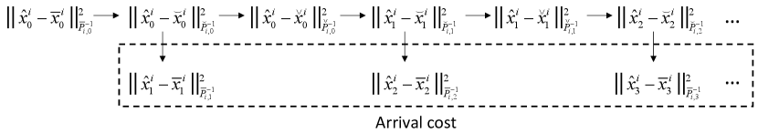
By iteratively applying the same procedure, the arrival cost Vki,oV_{k}^{i,o} for the subsequent sampling instants can be derived. Specifically, the recursive expression of the arrival cost Vki,oV_{k}^{i,o} for the iith subsystem is presented as follows:

Vki,o=x^kix¯kiPi,k12V_{k}^{i,o}=\|\hat{x}_{k}^{i}-\bar{x}_{k}^{i}\|^{2}_{P_{i,k}^{-1}} (24)

where the update of arrival cost has three steps, as illustrated in Figure 1. The details of the three steps are as follows:

  • From x^kix˘kiP˘i,k12\|\hat{x}_{k}^{i}-\breve{x}_{k}^{i}\|^{2}_{\breve{P}_{i,k}^{-1}} to x^kixˇkiPˇi,k12\|\hat{x}_{k}^{i}-\check{x}_{k}^{i}\|^{2}_{\check{P}_{i,k}^{-1}}:

    Pˇi,k\displaystyle\check{P}_{i,k} =P˘i,kP˘i,kA[:,i]TCT(CA[:,i]P˘i,kA[:,i]TCT+R)1CA[:,i]P˘i,k\displaystyle=\breve{P}_{i,k}-\breve{P}_{i,k}A_{[:,i]}^{\mathrm{T}}C^{\mathrm{T}}(CA_{[:,i]}\breve{P}_{i,k}A_{[:,i]}^{\mathrm{T}}C^{\mathrm{T}}+R)^{-1}CA_{[:,i]}\breve{P}_{i,k} (25a)
    xˇki\displaystyle\check{x}_{k}^{i} =x˘ki+P˘i,kA[:,i]TCT(CA[:,i]P˘i,kA[:,i]TCT+R)1(ykC(A[:,i]x˘k1i+l𝕀{i}A[:,l]x~k1l))\displaystyle=\breve{x}_{k}^{i}+\breve{P}_{i,k}A_{[:,i]}^{\mathrm{T}}C^{\mathrm{T}}(CA_{[:,i]}\breve{P}_{i,k}A_{[:,i]}^{\mathrm{T}}C^{\mathrm{T}}+R)^{-1}(y_{k}-C(A_{[:,i]}\breve{x}_{k-1}^{i}+\sum_{l\in\mathbb{I}\setminus\{i\}}A_{[:,l]}\tilde{x}_{k-1}^{l})) (25b)
  • From x^kixˇkiPˇi,k12\|\hat{x}_{k}^{i}-\check{x}_{k}^{i}\|^{2}_{\check{P}_{i,k}^{-1}} to x^k+1ix˘k+1iP˘i,k+112\|\hat{x}_{k+1}^{i}-\breve{x}_{k+1}^{i}\|^{2}_{\breve{P}_{i,k+1}^{-1}}:

    P˘i,k+1\displaystyle\breve{P}_{i,k+1} =Qi+AiiPˇi,kAiiT\displaystyle=Q_{i}+A_{ii}\check{P}_{i,k}A_{ii}^{\mathrm{T}} (25c)
    x˘k+1i\displaystyle\breve{x}_{k+1}^{i} =Aiixˇki+l𝕀{i}Ailx~kl\displaystyle=A_{ii}\check{x}_{k}^{i}+\sum_{l\in\mathbb{I}\setminus\{i\}}A_{il}\tilde{x}^{l}_{k} (25d)
  • From x^kix˘kiP˘i,k12\|\hat{x}_{k}^{i}-\breve{x}_{k}^{i}\|^{2}_{\breve{P}_{i,k}^{-1}} to the arrival cost x^k+1ix¯k+1iPi,k+112\|\hat{x}_{k+1}^{i}-\bar{x}_{k+1}^{i}\|^{2}_{{P}_{i,k+1}^{-1}}:

    Pi,k+1\displaystyle P_{i,k+1} =Qi+AiiP˘i,kAiiT\displaystyle=Q_{i}+A_{ii}\breve{P}_{i,k}A_{ii}^{\mathrm{T}} (25e)
    x¯k+1i\displaystyle\bar{x}_{k+1}^{i} =Aiix˘ki+l𝕀{i}Ailx~kl\displaystyle=A_{ii}\breve{x}_{k}^{i}+\sum_{l\in\mathbb{I}\setminus\{i\}}A_{il}\tilde{x}^{l}_{k} (25f)

By leveraging the arrival cost obtained in (25), the proposed DMHE design for the linear system in (4) is completed. Specifically, at sampling instant kk, the iith estimator of the proposed DMHE algorithm solves an optimization problem as follows:

min{x^ji}j=kNkj=kNk1w^jiQi12+j=kNkv^j[i]R12+x^kNix¯kNiPi,kN12\displaystyle\min_{\{\hat{x}^{i}_{j}\}_{j=k-N}^{k}}\sum_{j=k-N}^{k-1}\|\hat{w}^{i}_{j}\|^{2}_{Q_{i}^{-1}}+\sum_{j=k-N}^{k}\|\hat{v}^{[i]}_{j}\|^{2}_{R^{-1}}+\|\hat{x}^{i}_{k-N}-\bar{x}^{i}_{k-N}\|_{P_{i,k-N}^{-1}}^{2}
s.t.x^j+1i=Aiix^ji+l𝕀{i}Ailx~jl+w^ji\displaystyle\quad\quad\mathrm{s.t.}~{}\hat{x}_{j+1}^{i}=A_{ii}\hat{x}_{j}^{i}+\sum_{l\in\mathbb{I}\setminus\{i\}}A_{il}\tilde{x}_{j}^{l}+\hat{w}_{j}^{i} (26a)
ykN=C[:,i]x^kNi+l𝕀{i}C[:,l]x~kNl+v^kN[i]\displaystyle\quad\quad\quad~{}~{}y_{k-N}=C_{[:,i]}\hat{x}_{k-N}^{i}+\sum_{l\in\mathbb{I}\setminus\{i\}}C_{[:,l]}\tilde{x}_{k-N}^{l}+\hat{v}_{k-N}^{[i]} (26b)
yj+1=C(A[:,i]x^ji+l𝕀{i}A[:,l]x~jl)+vj+1[i],j=kN,,k1\displaystyle\quad\quad\quad~{}~{}y_{j+1}=C(A_{[:,i]}\hat{x}_{j}^{i}+\sum_{l\in\mathbb{I}\setminus\{i\}}A_{[:,l]}\tilde{x}_{j}^{l})+v_{j+1}^{[i]},~{}j=k-N,\ldots,k-1 (26c)
x^ki𝕏i\displaystyle\quad\quad\quad~{}~{}\hat{x}_{k}^{i}\in\mathbb{X}^{i} (26d)

In (26), w^jiQi12\|\hat{w}^{i}_{j}\|^{2}_{Q_{i}^{-1}} penalizes the deviation of estimated subsystem states from the nominal process subsystem model over an estimation window, ensuring that the state estimates can follow the system dynamics. v^j[i]R12\|\hat{v}^{[i]}_{j}\|^{2}_{R^{-1}} penalizes the discrepancy between the predicted measurements and actual measurements to ensure that the estimated states comply with measured outputs. The arrival cost x^kNix¯kNiPi,kN12\|\hat{x}^{i}_{k-N}-\bar{x}^{i}_{k-N}\|_{P_{i,k-N}^{-1}}^{2} summarizes the previous information that is not considered within the current estimation window.

4.2 Stability analysis

In this section, inspired by [30], we perform the stability analysis for the proposed DMHE method in (26), where the arrival costs of local estimators are approximated using a recursive approach for linear systems in (4) with state constraints. Before proceeding further, we introduce several matrices and one lemma as follows:

Ai\displaystyle A_{i}^{*} =[A1iAni],A~i=[A11A1,i10A1,i+1A1nAn1An,i10An,i+1Ann],Ci=[0Cii0],\displaystyle=\left[\begin{array}[]{c}A_{1i}\\ \vdots\\ A_{ni}\end{array}\right],\tilde{A}_{i}=\left[\begin{array}[]{ccccccc}A_{11}&\cdots&A_{1,i-1}&0&A_{1,i+1}&\cdots&A_{1n}\\ \vdots&&\vdots&\vdots&\vdots&&\vdots\\ A_{n1}&\cdots&A_{n,i-1}&0&A_{n,i+1}&\cdots&A_{nn}\\ \end{array}\right],C_{i}^{*}=\left[\begin{array}[]{c}0\\ \vdots\\ C_{ii}\\ \vdots\\ 0\end{array}\right],
C~i\displaystyle\tilde{C}_{i} =diag{C11,,Ci1,i1,0,Ci+1,i+1,,Cnn}\displaystyle=\mathrm{diag}\{C_{11},\ldots,C_{i-1,i-1},0,C_{i+1,i+1},\ldots,C_{nn}\}
Lemma 3.

([30]) If the rank of matrix CC is equal to the dimension of vector aa, then it holds that

CxaA12=xbCTA1C2\|Cx-a\|^{2}_{A^{-1}}=\|x-b\|^{2}_{C^{\mathrm{T}}A^{-1}C}

where b=(CTA1C)1CTA1ab=(C^{\mathrm{T}}A^{-1}C)^{-1}C^{\mathrm{T}}A^{-1}a.

To establish the stability of the proposed DMHE algorithm, we modify the objective function of (26) by incorporating a constant term Φk1i,\Phi^{i,*}_{k-1} and rewrite the iith estimator of the proposed DMHE method in (26). Specifically, at sampling instant kk, the iith estimator of the proposed DMHE approach in (26) can be written as:

Φki,=min{x^ji}j=kNkΦki,MHE\displaystyle\quad\quad\Phi^{i,*}_{k}=\min_{\{\hat{x}^{i}_{j}\}_{j=k-N}^{k}}\Phi^{i,\mathrm{MHE}}_{k}
s.t.x^j+1i=Aiix^ji+l𝕀{i}Ailx~jl+w^ji\displaystyle\mathrm{s.t.}~{}\,\hat{x}_{j+1}^{i}=A_{ii}\hat{x}_{j}^{i}+\sum_{l\in\mathbb{I}\setminus\{i\}}A_{il}\tilde{x}_{j}^{l}+\hat{w}_{j}^{i} (27a)
ykN=Cix^kNi+C~ix~kN+v^kN[i]\displaystyle\quad~{}~{}y_{k-N}=C^{*}_{i}\hat{x}_{k-N}^{i}+\tilde{C}_{i}\tilde{x}_{k-N}+\hat{v}_{k-N}^{[i]} (27b)
yj+1=C(Aix^ji+A~ix~j)+v^j+1[i],j=kN,,k1\displaystyle\quad~{}~{}~{}\,y_{j+1}=C(A^{*}_{i}\hat{x}_{j}^{i}+\tilde{A}_{i}\tilde{x}_{j})+\hat{v}_{j+1}^{[i]},~{}j=k-N,\ldots,k-1 (27c)
x^ki𝕏i\displaystyle\quad~{}~{}\quad~{}\hat{x}_{k}^{i}\in\mathbb{X}^{i} (27d)
where
Φki,MHE=j=kNk1w^jiQi12+j=kNkv^j[i]R12+x^kNix¯kNiPi,kN12+Φk1i,\Phi^{i,\mathrm{MHE}}_{k}=\sum_{j=k-N}^{k-1}\|\hat{w}^{i}_{j}\|^{2}_{Q_{i}^{-1}}+\sum_{j=k-N}^{k}\|\hat{v}^{[i]}_{j}\|^{2}_{R^{-1}}+\|\hat{x}^{i}_{k-N}-\bar{x}^{i}_{k-N}\|_{P_{i,k-N}^{-1}}^{2}+\Phi^{i,*}_{k-1} (27e)

where Φk1i,\Phi^{i,*}_{k-1} is the optimal value of the iith estimator of the proposed DMHE approach calculated at sampling instant k1k-1. The inclusion of the constant Φk1i,\Phi^{i,*}_{k-1} ensures that the sequence {Φki,}\{\Phi_{k}^{i,*}\} is non-decreasing. By leveraging the monotonicity and boundedness of {Φki,}\{\Phi_{k}^{i,*}\}, the sequence {Φki,}\{\Phi_{k}^{i,*}\} is convergent, as demonstrated in the proof of Proposition 2. This convergence forms the basis for proving the stability of the proposed linear DMHE algorithm in Theorem 1. It is noted that Φk1i,\Phi^{i,*}_{k-1} is a known value at sampling instant kk and can be disregarded when solving the optimization problem (27). Therefore, the reformulated DMHE method in (27) is equivalent to the proposed DMHE design in (26).

By creating augmented vectors x^j=col{x^j1,,x^jn}\hat{x}_{j}=\mathrm{col}\{\hat{x}_{j}^{1},\ldots,\hat{x}_{j}^{n}\}, x~j=col{x~j1,,x~jn}\tilde{x}_{j}=\mathrm{col}\{\tilde{x}_{j}^{1},\ldots,\tilde{x}_{j}^{n}\}, w^j=col{w^j1,,w^jn}\hat{w}_{j}=\mathrm{col}\{\hat{w}_{j}^{1},\ldots,\hat{w}_{j}^{n}\}, Yj=col{yj,,yjn}Y_{j}=\mathrm{col}\{\underbrace{y_{j},\ldots,y_{j}}_{n}\}, and V^j=col{v^j[1],\hat{V}_{j}=\mathrm{col}\{\hat{v}_{j}^{[1]},\ldots, v^j[n]}\hat{v}_{j}^{[n]}\}. The subsystem model in (27a)-(27c) can be concatenated to form a compact collective estimation model:

x^j+1\displaystyle\hat{x}_{j+1} =Adx^j+Arx~j+w^j\displaystyle=A_{d}\hat{x}_{j}+A_{r}\tilde{x}_{j}+\hat{w}_{j} (28a)
YkN\displaystyle Y_{k-N} =Cx^kN+C~x~kN+V^kN\displaystyle=C^{*}\hat{x}_{k-N}+\tilde{C}\tilde{x}_{k-N}+\hat{V}_{k-N} (28b)
Yj+1\displaystyle Y_{j+1} =𝐂(Ax^j+A~x~j)+V^j+1,j=kN,,k1\displaystyle=\mathbf{C}(A^{*}\hat{x}_{j}+\tilde{A}\tilde{x}_{j})+\hat{V}_{j+1},~{}j=k-N,\ldots,k-1 (28c)

where Ad=diag{A11,,Ann}A_{d}=\mathrm{diag}\{A_{11},\ldots,A_{nn}\}; Ar=AAdA_{r}=A-A_{d}; C=diag{C1,,Cn}C^{*}=\mathrm{diag}\{C^{*}_{1},\ldots,C^{*}_{n}\}; C~=col{C~1,,C~n}\tilde{C}=\mathrm{col}\{\tilde{C}_{1},\ldots,\tilde{C}_{n}\}; 𝐂=diag{C,,Cn}\mathbf{C}=\mathrm{diag}\{\underbrace{C,\ldots,C}_{n}\}, A=diag{A1,,An}A^{*}=\mathrm{diag}\{A^{*}_{1},\ldots,A^{*}_{n}\}; A~=col{A~1,,A~n}\tilde{A}=\mathrm{col}\{\tilde{A}_{1},\ldots,\tilde{A}_{n}\}. We further define a collective form of the objective function by summarizing the local objective functions Φki,MHE\Phi^{i,\mathrm{MHE}}_{k} for all i𝕀i\in\mathbb{I}:

ΦkMHE\displaystyle\Phi_{k}^{\mathrm{MHE}} =i𝕀Φki,MHE\displaystyle=\sum_{i\in\mathbb{I}}\Phi^{i,\mathrm{MHE}}_{k}
=x^kNx¯kNPkN12+j=kNk1w^jQ12+j=kNkV^j𝐑12+Φk1\displaystyle=\|\hat{x}_{k-N}-\bar{x}_{k-N}\|^{2}_{P_{k-N}^{-1}}+\sum_{j=k-N}^{k-1}\|\hat{w}_{j}\|^{2}_{Q^{-1}}+\sum_{j=k-N}^{k}\|\hat{V}_{j}\|^{2}_{\mathbf{R}^{-1}}+\Phi^{*}_{k-1} (29)

where PkN=diag{P1,kN,,Pn,kN}P_{k-N}=\mathrm{diag}\{P_{1,k-N},\ldots,P_{n,k-N}\}; Q=diag{Q1,,Qn}Q=\mathrm{diag}\{Q_{1},\ldots,Q_{n}\}; 𝐑=diag{R,,Rn}\mathbf{R}=\mathrm{diag}\{\underbrace{R,\ldots,R}_{n}\}; Φk1=i𝕀Φk1i,\Phi^{*}_{k-1}=\sum_{i\in\mathbb{I}}\Phi^{i,*}_{k-1}. It is worth mentioning that the solution of the proposed DMHE design in (27) is equivalent to solving the following optimization problem:

Φk\displaystyle\Phi^{*}_{k} =min{x^j}j=kNkΦkMHEsubject to (28) and x^𝕏\displaystyle=\min_{\{\hat{x}_{j}\}_{j=k-N}^{k}}\Phi^{\mathrm{MHE}}_{k}~{}\text{subject to \eqref{collective_estimation} and }\hat{x}\in\mathbb{X} (30)

Similar to the stability analysis conducted in [30, 14], for a sequence zjinxiz_{j}^{i}\in\mathbb{R}^{n_{x^{i}}}, j=kN+1,,kj=k-N+1,\ldots,k, we define the transit cost Φ[kN+1,k]/ki,MHE({zji}j=kN+1k)\Phi^{i,\mathrm{MHE}}_{[k-N+1,k]/k}(\{z_{j}^{i}\}_{j=k-N+1}^{k}) of the proposed DMHE approach in (27) for the subsystem ii:

Φ[kN+1,k]/ki,MHE({zji}j=kN+1k)\displaystyle\Phi^{i,\mathrm{MHE}}_{[k-N+1,k]/k}(\{z_{j}^{i}\}_{j=k-N+1}^{k}) =min{x^ji}j=kNkΦki,MHEsubject to (27) and x^ji=zjiforj=kN+1,,k\displaystyle=\min_{\{\hat{x}^{i}_{j}\}_{j=k-N}^{k}}\Phi^{i,\mathrm{MHE}}_{k}~{}\text{subject to \eqref{dmhe_revised} and~{}}\hat{x}_{j}^{i}=z_{j}^{i}~{}\text{for}~{}j=k-N+1,\ldots,k (31)

Let zj=col{zj1,,zjn}nxz_{j}=\mathrm{col}\{z_{j}^{1},\ldots,z_{j}^{n}\}\in\mathbb{R}^{n_{x}}, the collective transit cost of (30) takes the following form:

Φ[kN+1,k]/kMHE({zj}j=kN+1k)\displaystyle\Phi^{\mathrm{MHE}}_{[k-N+1,k]/k}(\{z_{j}\}_{j=k-N+1}^{k}) =min{x^j}j=kNkΦkMHEsubject to (28) andx^j=zjforj=kN+1,,k\displaystyle=\min_{\{\hat{x}_{j}\}_{j=k-N}^{k}}\Phi^{\mathrm{MHE}}_{k}~{}\text{subject to \eqref{collective_estimation} and}~{}\hat{x}_{j}=z_{j}~{}\text{for}~{}j=k-N+1,\ldots,k

such that

Φ[kN+1,k]/kMHE({zj}j=kN+1k)=i𝕀Φ[kN+1,k]/ki,MHE({zji}j=kN+1k)\Phi^{\mathrm{MHE}}_{[k-N+1,k]/k}(\{z_{j}\}_{j=k-N+1}^{k})=\sum_{i\in\mathbb{I}}\Phi^{i,\mathrm{MHE}}_{[k-N+1,k]/k}(\{z_{j}^{i}\}_{j=k-N+1}^{k})

Before introducing Proposition 1 and Lemma 4, an unconstrained DMHE design is formulated as follows:

Φki,u\displaystyle\Phi^{i,u}_{k} =min{x^ji}j=kNkΦki,MHEsubject to (27a)-(27c)\displaystyle=\min_{\{\hat{x}^{i}_{j}\}_{j=k-N}^{k}}\Phi^{i,\mathrm{MHE}}_{k}~{}\text{subject to \eqref{eq:dmhe_1}-\eqref{eq:dmhe_3}} (32)

The associated transit cost of the unconstrained DMHE approach in (32) for the iith subsystem is described as follows:

Φ[kN+1,k]/ki,u({zji}j=kN+1k)\displaystyle\Phi^{i,u}_{[k-N+1,k]/k}(\{z_{j}^{i}\}_{j=k-N+1}^{k}) =min{x^ji}j=kNkΦki,MHEsubject to (27a)-(27c)\displaystyle=\min_{\{\hat{x}^{i}_{j}\}_{j=k-N}^{k}}\Phi^{i,\mathrm{MHE}}_{k}~{}\text{subject to \eqref{eq:dmhe_1}-\eqref{eq:dmhe_3}}
andx^ji=zjiforj=kN+1,,k\displaystyle\quad\text{and}~{}\hat{x}_{j}^{i}=z_{j}^{i}~{}\text{for}~{}j=k-N+1,\ldots,k (33)
Proposition 1.

Let {x^ji,u}j=kNk\{\hat{x}_{j}^{i,u}\}_{j=k-N}^{k} be the solution of the unconstrained DMHE problem in (32) for the subsystem ii. Then there exist a positive-define matrix HkiH^{i}_{k}, such that the transit cost Φ[kN+1,k]/ki,u\Phi^{i,u}_{[k-N+1,k]/k} ({zji}j=kN+1k)(\{z_{j}^{i}\}_{j=k-N+1}^{k}) in (4.2) is given by the following equation:

Φ[kN+1,k]/ki,u({zji}j=kN+1k)={zji}j=kN+1k{x^ji,u}j=kN+1kHki2+Φki,u\Phi^{i,u}_{[k-N+1,k]/k}(\{z_{j}^{i}\}_{j=k-N+1}^{k})=\|\{z_{j}^{i}\}_{j=k-N+1}^{k}-\{\hat{x}_{j}^{i,u}\}_{j=k-N+1}^{k}\|^{2}_{H^{i}_{k}}+\Phi^{i,u}_{k}

Proof.

Based on (27e), substituting the constraints (27a)-(27c) and the constraints x^ji=zji\hat{x}_{j}^{i}=z_{j}^{i} for j=kN+1,,kj=k-N+1,\ldots,k, into Φki,MHE\Phi_{k}^{i,\mathrm{MHE}} yields:

j=kN+1k1zj+1iAiizjilI{i}Ailx~jlQi12+j=kN+1k1yj+1C(Aizji+A~ix~j)R12\displaystyle\sum_{j=k-N+1}^{k-1}\|z_{j+1}^{i}-A_{ii}z_{j}^{i}-\sum_{l\in\mathrm{I}\setminus\{i\}}A_{il}\tilde{x}_{j}^{l}\|^{2}_{Q_{i}^{-1}}+\sum_{j=k-N+1}^{k-1}\|y_{j+1}-C(A_{i}^{*}z_{j}^{i}+\tilde{A}_{i}\tilde{x}_{j})\|^{2}_{R^{-1}}
+\displaystyle+ zkN+1iAiix^kNilI{i}Ailx~kNlQi12+ykN+1C(Aix^kNi+A~ix~kN)R12\displaystyle\|z_{k-N+1}^{i}-A_{ii}\hat{x}_{k-N}^{i}-\sum_{l\in\mathrm{I}\setminus\{i\}}A_{il}\tilde{x}_{k-N}^{l}\|^{2}_{Q_{i}^{-1}}+\|y_{k-N+1}-C(A_{i}^{*}\hat{x}_{k-N}^{i}+\tilde{A}_{i}\tilde{x}_{k-N})\|^{2}_{R^{-1}}
+\displaystyle+ ykNCix^kNiC~ix~kNR12+x^kNix¯kNiPi,kN12+Φk1i,\displaystyle\|y_{k-N}-C_{i}^{*}\hat{x}_{k-N}^{i}-\tilde{C}_{i}\tilde{x}_{k-N}\|^{2}_{R^{-1}}+\|\hat{x}_{k-N}^{i}-\bar{x}_{k-N}^{i}\|^{2}_{P_{i,k-N}^{-1}}+\Phi_{k-1}^{i,*} (34)

From Lemma 1, it holds that

ykNCix^kNiC~ix~kNR12+x^kNix¯kNiPi,kN12\displaystyle\quad\|y_{k-N}-C_{i}^{*}\hat{x}_{k-N}^{i}-\tilde{C}_{i}\tilde{x}_{k-N}\|^{2}_{R^{-1}}+\|\hat{x}_{k-N}^{i}-\bar{x}_{k-N}^{i}\|^{2}_{P_{i,k-N}^{-1}}
=x^kNix˘kNiP˘i,kN12+const\displaystyle=\|\hat{x}_{k-N}^{i}-\breve{x}_{k-N}^{i}\|^{2}_{\breve{P}_{i,k-N}^{-1}}+\text{const} (35)

where

P˘i,kN\displaystyle\breve{P}_{i,k-N} =Pi,kNPi,kN(Ci)T(CiPi,kN(Ci)T+R)1CiPi,kN\displaystyle=P_{i,k-N}-P_{i,k-N}(C_{i}^{*})^{\mathrm{T}}(C_{i}^{*}P_{i,k-N}(C_{i}^{*})^{\mathrm{T}}+R)^{-1}C_{i}^{*}P_{i,k-N}
x˘kNi\displaystyle\breve{x}_{k-N}^{i} =x¯kNi+Pi,kN(Ci)T(CiPi,kN(Ci)T+R)1(ykNCix¯kNiC~ix~kN)\displaystyle=\bar{x}_{k-N}^{i}+P_{i,k-N}(C_{i}^{*})^{\mathrm{T}}(C_{i}^{*}P_{i,k-N}(C_{i}^{*})^{\mathrm{T}}+R)^{-1}(y_{k-N}-C_{i}^{*}\bar{x}_{k-N}^{i}-\tilde{C}_{i}\tilde{x}_{k-N})

constconst represents a constant, which will be defined later. Similarly, it is further obtained:

x^kNix˘kNiP˘i,kN12+ykN+1C(Aix^kNi+A~ix~kN)R12\displaystyle\quad\|\hat{x}_{k-N}^{i}-\breve{x}_{k-N}^{i}\|^{2}_{\breve{P}_{i,k-N}^{-1}}+\|y_{k-N+1}-C(A_{i}^{*}\hat{x}_{k-N}^{i}+\tilde{A}_{i}\tilde{x}_{k-N})\|^{2}_{R^{-1}}
=x^kNixˇkNiPˇi,kN12+const\displaystyle=\|\hat{x}_{k-N}^{i}-\check{x}_{k-N}^{i}\|^{2}_{\check{P}_{i,k-N}^{-1}}+\text{const} (36)

where

Pˇi,kN\displaystyle\check{P}_{i,k-N} =P˘i,kNP˘i,kN(Ai)TCT(CAiP˘i,kN(Ai)TCT+R)1CAiP˘i,kN\displaystyle=\breve{P}_{i,k-N}-\breve{P}_{i,k-N}(A_{i}^{*})^{\mathrm{T}}C^{\mathrm{T}}(CA_{i}^{*}\breve{P}_{i,k-N}(A_{i}^{*})^{\mathrm{T}}C^{\mathrm{T}}+R)^{-1}CA_{i}^{*}\breve{P}_{i,k-N}
xˇkNi\displaystyle\check{x}_{k-N}^{i} =x˘kNi+P˘i,kN(Ai)TCT(CAiP˘i,kN(Ai)TCT+R)1(ykN+1C(Aix˘kNi+A~ix~kN))\displaystyle=\breve{x}_{k-N}^{i}+\breve{P}_{i,k-N}(A_{i}^{*})^{\mathrm{T}}C^{\mathrm{T}}(CA_{i}^{*}\breve{P}_{i,k-N}(A_{i}^{*})^{\mathrm{T}}C^{\mathrm{T}}+R)^{-1}(y_{k-N+1}-C(A_{i}^{*}\breve{x}_{k-N}^{i}+\tilde{A}_{i}\tilde{x}_{k-N}))

and

x^kNixˇkNiPˇi,kN12+zkN+1iAiix^kNilI{i}Ailx~kNlQi12\displaystyle\quad\|\hat{x}_{k-N}^{i}-\check{x}_{k-N}^{i}\|^{2}_{\check{P}_{i,k-N}^{-1}}+\|z_{k-N+1}^{i}-A_{ii}\hat{x}_{k-N}^{i}-\sum_{l\in\mathrm{I}\setminus\{i\}}A_{il}\tilde{x}_{k-N}^{l}\|^{2}_{Q_{i}^{-1}}
=x^kNiσH12+zkN+1iAiixˇkNilI{i}Ailx~kNlPi,kN+112\displaystyle=\|\hat{x}_{k-N}^{i}-\sigma\|^{2}_{H^{-1}}+\|z_{k-N+1}^{i}-A_{ii}\check{x}_{k-N}^{i}-\sum_{l\in\mathrm{I}\setminus\{i\}}A_{il}\tilde{x}_{k-N}^{l}\|^{2}_{P_{i,k-N+1}^{-1}} (37)

where

H\displaystyle H =Pˇi,kNAiiT(AiiPˇi,kNAiiT+Qi)1\displaystyle=\check{P}_{i,k-N}A_{ii}^{\mathrm{T}}(A_{ii}\check{P}_{i,k-N}A_{ii}^{\mathrm{T}}+Q_{i})^{-1}
σ\displaystyle\sigma =xˇkNi+Pˇi,kNAiiT(AiiPˇi,kNAiiT+Qi)1(zkN+1iAiixˇkNilI{i}Ailx~kNl)\displaystyle=\check{x}_{k-N}^{i}+\check{P}_{i,k-N}A_{ii}^{\mathrm{T}}(A_{ii}\check{P}_{i,k-N}A_{ii}^{\mathrm{T}}+Q_{i})^{-1}(z_{k-N+1}^{i}-A_{ii}\check{x}_{k-N}^{i}-\sum_{l\in\mathrm{I}\setminus\{i\}}A_{il}\tilde{x}_{k-N}^{l})
Pi,kN+1\displaystyle P_{i,k-N+1} =Qi+AiiPˇi,kNAiiT\displaystyle=Q_{i}+A_{ii}\check{P}_{i,k-N}A_{ii}^{\mathrm{T}}

Therefore, by substituting (Proof), (Proof), and (Proof) into (Proof), we have

Φ[kN+1,k]/ki,u({zji}j=kN+1k)\displaystyle\quad\Phi^{i,u}_{[k-N+1,k]/k}(\{z_{j}^{i}\}_{j=k-N+1}^{k})
=minx^kNi{j=kN+1k1zj+1iAiizjilI{i}Ailx~jlQi12+j=kN+1k1yj+1C(Aizji+A~ix~j)R12\displaystyle=\min_{\hat{x}^{i}_{k-N}}\Big{\{}\sum_{j=k-N+1}^{k-1}\|z_{j+1}^{i}-A_{ii}z_{j}^{i}-\sum_{l\in\mathrm{I}\setminus\{i\}}A_{il}\tilde{x}_{j}^{l}\|^{2}_{Q_{i}^{-1}}+\sum_{j=k-N+1}^{k-1}\|y_{j+1}-C(A_{i}^{*}z_{j}^{i}+\tilde{A}_{i}\tilde{x}_{j})\|^{2}_{R^{-1}}
+x^kNiσH12+zkN+1iAiixˇkNilI{i}Ailx~kNlPi,kN+112+const}\displaystyle\quad+\|\hat{x}_{k-N}^{i}-\sigma\|^{2}_{H^{-1}}+\|z_{k-N+1}^{i}-A_{ii}\check{x}_{k-N}^{i}-\sum_{l\in\mathrm{I}\setminus\{i\}}A_{il}\tilde{x}_{k-N}^{l}\|^{2}_{P_{i,k-N+1}^{-1}}+\text{const}\Big{\}} (38)

It is noted that the optimal solution of (Proof) is x^kNi=σ\hat{x}_{k-N}^{i}=\sigma. Consequently, we can obtain that

Φ[kN+1,k]/ki,u({zji}j=kN+1k)\displaystyle\quad\Phi^{i,u}_{[k-N+1,k]/k}(\{z_{j}^{i}\}_{j=k-N+1}^{k})
=j=kN+1k1zj+1iAiizjilI{i}Ailx~jlQi12+j=kN+1k1yj+1C(Aizji+A~ix~j)R12\displaystyle=\sum_{j=k-N+1}^{k-1}\|z_{j+1}^{i}-A_{ii}z_{j}^{i}-\sum_{l\in\mathrm{I}\setminus\{i\}}A_{il}\tilde{x}_{j}^{l}\|^{2}_{Q_{i}^{-1}}+\sum_{j=k-N+1}^{k-1}\|y_{j+1}-C(A_{i}^{*}z_{j}^{i}+\tilde{A}_{i}\tilde{x}_{j})\|^{2}_{R^{-1}}
+zkN+1iAiixˇkNilI{i}Ailx~kNlPi,kN+112+const\displaystyle\quad+\|z_{k-N+1}^{i}-A_{ii}\check{x}_{k-N}^{i}-\sum_{l\in\mathrm{I}\setminus\{i\}}A_{il}\tilde{x}_{k-N}^{l}\|^{2}_{P_{i,k-N+1}^{-1}}+\text{const} (39)

Define Y1,i=AiixˇkNi+lI{i}Ailx~kNlY_{1,i}=A_{ii}\check{x}_{k-N}^{i}+\sum_{l\in\mathrm{I}\setminus\{i\}}A_{il}\tilde{x}_{k-N}^{l},

Y2,i\displaystyle Y_{2,i} =[lI{i}Ailx~kN+1llI{i}Ailx~k1l],Y3,i=[ykN+2CA~ix~kN+1ykCA~ix~k1],C1,i=[Inxi,0,,0N1],\displaystyle=\left[\begin{array}[]{ccc}\sum_{l\in\mathrm{I}\setminus\{i\}}A_{il}\tilde{x}_{k-N+1}^{l}\\ \vdots\\ \sum_{l\in\mathrm{I}\setminus\{i\}}A_{il}\tilde{x}_{k-1}^{l}\end{array}\right],~{}Y_{3,i}=\left[\begin{array}[]{ccc}y_{k-N+2}-C\tilde{A}_{i}\tilde{x}_{k-N+1}\\ \vdots\\ y_{k}-C\tilde{A}_{i}\tilde{x}_{k-1}\end{array}\right],C_{1,i}=[I_{n_{x^{i}}},\underbrace{0,\ldots,0}_{N-1}],
C2,i\displaystyle C_{2,i} =[AiiInxi0000AiiInxi00000AiiInxi],C3,i=[CAi0000CAi0000CAi0]\displaystyle=\left[\begin{array}[]{ccccccccc}-A_{ii}&I_{n_{x^{i}}}&0&\ldots&0&0\\ 0&-A_{ii}&I_{n_{x^{i}}}&\ldots&0&0\\ \vdots&\vdots&\vdots&\ddots&\vdots&\vdots\\ 0&0&0&\ldots&-A_{ii}&I_{n_{x^{i}}}\\ \end{array}\right],C_{3,i}=\left[\begin{array}[]{ccccccc}CA_{i}^{*}&0&\ldots&0&0\\ 0&CA_{i}^{*}&\ldots&0&0\\ \vdots&\vdots&\ddots&\vdots&\vdots\\ 0&0&\ldots&CA_{i}^{*}&0\\ \end{array}\right]

Consequently, (Proof) can be rewritten as

Φ[kN+1,k]/ki,u({zji}j=kN+1k)\displaystyle\Phi^{i,u}_{[k-N+1,k]/k}(\{z_{j}^{i}\}_{j=k-N+1}^{k}) =C1,i{zji}j=kN+1kY1,iPi,kN+112+C2,i{zji}j=kN+1kY2,i𝐐i12\displaystyle=\|C_{1,i}\{z_{j}^{i}\}_{j=k-N+1}^{k}-Y_{1,i}\|^{2}_{P_{i,k-N+1}^{-1}}+\|C_{2,i}\{z_{j}^{i}\}_{j=k-N+1}^{k}-Y_{2,i}\|^{2}_{\mathbf{Q}_{i}^{-1}}
+C3,i{zji}j=kN+1kY3,i𝐑12+const\displaystyle\quad+\|C_{3,i}\{z_{j}^{i}\}_{j=k-N+1}^{k}-Y_{3,i}\|^{2}_{\mathbf{R}^{-1}}+\text{const}
=C4,i{zji}j=kN+1kY4,i(H~ki)12+const\displaystyle=\|C_{4,i}\{z_{j}^{i}\}_{j=k-N+1}^{k}-Y_{4,i}\|^{2}_{(\tilde{H}_{k}^{i})^{-1}}+\text{const} (40)

where 𝐐i=diag{Qi,,QiN1}\mathbf{Q}_{i}=\mathrm{diag}\{\underbrace{Q_{i},\ldots,Q_{i}}_{N-1}\}; 𝐑=diag{R,,RN1}\mathbf{R}=\mathrm{diag}\{\underbrace{R,\ldots,R}_{N-1}\}; Y4,i=col{Y1,i,Y2,i,Y3,i}Y_{4,i}=\mathrm{col}\{Y_{1,i},Y_{2,i},Y_{3,i}\}; C4,i=col{C1,i,C2,i,C3,i}C_{4,i}=\mathrm{col}\{C_{1,i},C_{2,i},C_{3,i}\}; H~ki=diag{Pi,kN+1,𝐐i,𝐑}\tilde{H}_{k}^{i}=\mathrm{diag}\{P_{i,k-N+1},\mathbf{Q}_{i},\mathbf{R}\}. According to Lemma 3, (Proof) is equivalent to the equation

Φ[kN+1,k]/ki,u({zji}j=kN+1k)={zji}j=kN+1kYiHki2+const\Phi^{i,u}_{[k-N+1,k]/k}(\{z_{j}^{i}\}_{j=k-N+1}^{k})=\|\{z_{j}^{i}\}_{j=k-N+1}^{k}-Y_{i}\|^{2}_{H_{k}^{i}}+\text{const} (41)

where

Hki\displaystyle H_{k}^{i} =C4,iT(H~ki)1C4,i\displaystyle=C_{4,i}^{\mathrm{T}}(\tilde{H}_{k}^{i})^{-1}C_{4,i} (42a)
Yi\displaystyle Y_{i} =(C4,iT(H~ki)1C4,i)1C4,iT(H~ki)1Y4,i\displaystyle=(C_{4,i}^{\mathrm{T}}(\tilde{H}_{k}^{i})^{-1}C_{4,i})^{-1}C_{4,i}^{\mathrm{T}}(\tilde{H}_{k}^{i})^{-1}Y_{4,i} (42b)

By optimality, zji=x^ji,uz_{j}^{i}=\hat{x}_{j}^{i,u}, where j=kN+1,,kj=k-N+1,\ldots,k, are the global minimizers of transit cost Φ[kN+1,k]/ki,u({zji}j=kN+1k)\Phi^{i,u}_{[k-N+1,k]/k}(\{z_{j}^{i}\}_{j=k-N+1}^{k}) in (4.2), and the corresponding global minimum of the transit cost in (4.2) is Φki,u\Phi_{k}^{i,u}. Therefore, we have that {x^ji,u}j=kN+1k=Yi\{\hat{x}_{j}^{i,u}\}_{j=k-N+1}^{k}=Y_{i}, and the constant term in (41) is Φki,u\Phi_{k}^{i,u}. \square

Lemma 4.

([30]) Let {x^ji}j=kNk\{\hat{x}_{j}^{i}\}_{j=k-N}^{k} be the solution of the proposed DMHE problem in (27) for the subsystem ii. Then it holds

Φ[kN+1,k]/ki,MHE({zji}j=kN+1k){zji}j=kN+1k{x^ji}j=kN+1kHki2+Φki,\Phi^{i,\mathrm{MHE}}_{[k-N+1,k]/k}(\{z_{j}^{i}\}_{j=k-N+1}^{k})\geq\|\{z_{j}^{i}\}_{j=k-N+1}^{k}-\{\hat{x}_{j}^{i}\}_{j=k-N+1}^{k}\|^{2}_{H_{k}^{i}}+\Phi^{i,*}_{k}

Before proceeding further, we introduce a matrix and an assumption that will be used to prove the stability of the proposed DMHE method in (27).

Wki\displaystyle W_{k}^{i} =diag{Pl,kN1+CTR1C+ni𝕀(Ar,ilTQi1Ar,il+A~i,[:,i]TCTR1CA~i,[:,i]),,\displaystyle=\mathrm{diag}\{P_{l,k-N}^{-1}+C^{\mathrm{T}}R^{-1}C+n\sum_{i\in\mathbb{I}}(A_{r,il}^{\mathrm{T}}Q_{i}^{-1}A_{r,il}+\tilde{A}_{i,[:,i]}^{\mathrm{T}}C^{\mathrm{T}}R^{-1}C\tilde{A}_{i,[:,i]}),\ldots,
ni𝕀(Ar,ilTQi1Ar,il+A~i,[:,i]TCTR1CA~i,[:,i])}\displaystyle\quad n\sum_{i\in\mathbb{I}}(A_{r,il}^{\mathrm{T}}Q_{i}^{-1}A_{r,il}+\tilde{A}_{i,[:,i]}^{\mathrm{T}}C^{\mathrm{T}}R^{-1}C\tilde{A}_{i,[:,i]})\} (43)
Assumption 1.

The matrices HkiH_{k}^{i} and WkiW_{k}^{i} satisfy

WkiHki,i𝕀W_{k}^{i}\leq H_{k}^{i},~{}\forall i\in\mathbb{I}

where HkiH_{k}^{i} and WkiW_{k}^{i} are defined in (42a) and (4.2), respectively.

Proposition 2.

For the proposed DMHE approach in (27), if Assumption 1 holds, then

j=kNk1w^jQi12+j=kNkV^j𝐑12k0\sum_{j=k-N}^{k-1}\|\hat{w}_{j}\|^{2}_{Q_{i}^{-1}}+\sum_{j=k-N}^{k}\|\hat{V}_{j}\|^{2}_{\mathbf{R}^{-1}}\mathop{\longrightarrow}\limits^{k\rightarrow\infty}0 (44)

Proof.

Based on (4.2) and (30), we can obtain the following

ΦkΦk1j=kNk1w^jQi12+j=kNkV^j𝐑120\Phi^{*}_{k}-\Phi^{*}_{k-1}\geq\sum_{j=k-N}^{k-1}\|\hat{w}_{j}\|^{2}_{Q_{i}^{-1}}+\sum_{j=k-N}^{k}\|\hat{V}_{j}\|^{2}_{\mathbf{R}^{-1}}\geq 0 (45)

Therefore, the sequence Φk\Phi^{*}_{k} is increasing. According to optimality Φk\Phi^{*}_{k}, it follows that

Φk\displaystyle\Phi^{*}_{k} Φ[kN+1,k]/kMHE({xj}j=kN+1k)\displaystyle\leq\Phi_{[k-N+1,k]/k}^{\mathrm{MHE}}(\{x_{j}\}_{j=k-N+1}^{k}) (46)

where xjx_{j}, j=kN+1,,kj=k-N+1,\ldots,k, is the actual state generated by (4) without process disturbances and measurement noise. From (28), by choosing x^kN=xkN\hat{x}_{k-N}=x_{k-N} and w^j=Ar(xjx~j)\hat{w}_{j}=A_{r}(x_{j}-\tilde{x}_{j}) for j=kN,,k1j=k-N,\ldots,k-1, the trajectory of x^j=xj\hat{x}_{j}=x_{j}, for j=kN+1,,kj=k-N+1,\ldots,k, can be generated. Then, we have

V^j={𝐂A~(xj1x~j1),forj=kN+1,,kC(xjx~j),forj=kN\normalsize\hat{V}_{j}=\left\{\begin{array}[]{l}\mathbf{C}\tilde{A}(x_{j-1}-\tilde{x}_{j-1}),~{}~{}~{}~{}~{}{\text{for}}~{}j=k-N+1,\ldots,k{}{}\\[3.00003pt] C^{*}(x_{j}-\tilde{x}_{j}),~{}~{}~{}~{}~{}~{}~{}~{}~{}~{}~{}{\text{for}}~{}j=k-N{}{}\end{array}\right. (47)

Therefore, by optimality, it holds that

Φ[kN+1,k]/kMHE({xj}j=kN+1k)\displaystyle\Phi_{[k-N+1,k]/k}^{\mathrm{MHE}}(\{x_{j}\}_{j=k-N+1}^{k}) j=kNk1Ar(xjx~j)Q12+j=kNk1𝐂A~(xjx~j)𝐑12\displaystyle\leq\sum_{j=k-N}^{k-1}\|A_{r}(x_{j}-\tilde{x}_{j})\|^{2}_{Q^{-1}}+\sum_{j=k-N}^{k-1}\|\mathbf{C}\tilde{A}(x_{j}-\tilde{x}_{j})\|^{2}_{\mathbf{R}^{-1}} (48)
+C(xkNx~kN)𝐑12+xkNx¯kNPkN12+Φk1\displaystyle\quad+\|C^{*}(x_{k-N}-\tilde{x}_{k-N})\|^{2}_{\mathbf{R}^{-1}}+\|x_{k-N}-\bar{x}_{k-N}\|^{2}_{P_{k-N}^{-1}}+\Phi^{*}_{k-1}

Next, our objective is to prove that Φ[kN+1,k]/kMHE({xj}j=kN+1k)Φ[kN,k1]/k1MHE({xj}j=kNk1)\Phi_{[k-N+1,k]/k}^{\mathrm{MHE}}(\{x_{j}\}_{j=k-N+1}^{k})\leq\Phi_{[k-N,k-1]/k-1}^{\mathrm{MHE}}(\{x_{j}\}_{j=k-N}^{k-1}). To achieve this, we analyze each term on the right-hand-side of (48). Specifically, the first term on the right-hand-side of (48) satisfies

j=kNk1Ar(xjx~j)Q12\displaystyle\sum_{j=k-N}^{k-1}\|A_{r}(x_{j}-\tilde{x}_{j})\|^{2}_{Q^{-1}} =i𝕀j=kNk1l𝕀Ar,il(xjlx~jl)Qi12\displaystyle=\sum_{i\in\mathbb{I}}\sum_{j=k-N}^{k-1}\|\sum_{l\in\mathbb{I}}A_{r,il}(x_{j}^{l}-\tilde{x}_{j}^{l})\|^{2}_{Q_{i}^{-1}}
i𝕀j=kNk1l𝕀nAr,il(xjlx~jl)Qi12\displaystyle\leq\sum_{i\in\mathbb{I}}\sum_{j=k-N}^{k-1}\sum_{l\in\mathbb{I}}n\|A_{r,il}(x_{j}^{l}-\tilde{x}_{j}^{l})\|^{2}_{Q_{i}^{-1}}
=l𝕀j=kNk1xjlx~jlni𝕀Ar,ilTQi1Ar,il2\displaystyle=\sum_{l\in\mathbb{I}}\sum_{j=k-N}^{k-1}\|x_{j}^{l}-\tilde{x}_{j}^{l}\|^{2}_{n\sum_{i\in\mathbb{I}}A_{r,il}^{\mathrm{T}}Q_{i}^{-1}A_{r,il}} (49)

where Ar,ilA_{r,il} represents the block matrix in the iith row and the llth column of the matrix ArA_{r}. Similarly, by analyzing the remaining terms on the right-hand-side of (48), one can obtain

j=kNk1𝐂A~(xjx~j)𝐑12\displaystyle\sum_{j=k-N}^{k-1}\|\mathbf{C}\tilde{A}(x_{j}-\tilde{x}_{j})\|^{2}_{\mathbf{R}^{-1}} l𝕀j=kNk1xjlx~jlni𝕀A~i,[:,i]TCTR1CA~i,[:,i]2\displaystyle\leq\sum_{l\in\mathbb{I}}\sum_{j=k-N}^{k-1}\|x_{j}^{l}-\tilde{x}_{j}^{l}\|^{2}_{n\sum_{i\in\mathbb{I}}\tilde{A}_{i,[:,i]}^{\mathrm{T}}C^{\mathrm{T}}R^{-1}C\tilde{A}_{i,[:,i]}} (50a)
𝐂(xkNx~kN)𝐑12\displaystyle\|\mathbf{C}(x_{k-N}-\tilde{x}_{k-N})\|^{2}_{\mathbf{R}^{-1}} l𝕀xkNlx~kNlCTR1C2\displaystyle\leq\sum_{l\in\mathbb{I}}\|x_{k-N}^{l}-\tilde{x}_{k-N}^{l}\|^{2}_{C^{\mathrm{T}}R^{-1}C} (50b)
xkNx¯kNPkN12\displaystyle\|x_{k-N}-\bar{x}_{k-N}\|^{2}_{P_{k-N}^{-1}} l𝕀xkNlx~kNlPl,kN12\displaystyle\leq\sum_{l\in\mathbb{I}}\|x_{k-N}^{l}-\tilde{x}_{k-N}^{l}\|^{2}_{P_{l,k-N}^{-1}} (50c)

where A~i,[:,i]\tilde{A}_{i,[:,i]} is composed of the columns of A~i\tilde{A}_{i} with respect to subsystem state xix^{i}. Then, substituting (Proof) and (50) into (48) yields

Φ[kN+1,k]/kMHE({xj}j=kN+1k)\displaystyle\Phi_{[k-N+1,k]/k}^{\mathrm{MHE}}(\{x_{j}\}_{j=k-N+1}^{k}) l𝕀xkNlx~kNlPl,kN1+CTR1C2\displaystyle\leq\sum_{l\in\mathbb{I}}\|x_{k-N}^{l}-\tilde{x}_{k-N}^{l}\|^{2}_{P_{l,k-N}^{-1}+C^{\mathrm{T}}R^{-1}C}
+l𝕀j=kNk1xjlx~jlni𝕀(Ar,ilTQi1Ar,il+A~i,[:,i]TCTR1CA~i,[:,i])2+Φk1\displaystyle\quad+\sum_{l\in\mathbb{I}}\sum_{j=k-N}^{k-1}\|x_{j}^{l}-\tilde{x}_{j}^{l}\|^{2}_{n\sum_{i\in\mathbb{I}}(A_{r,il}^{\mathrm{T}}Q_{i}^{-1}A_{r,il}+\tilde{A}_{i,[:,i]}^{\mathrm{T}}C^{\mathrm{T}}R^{-1}C\tilde{A}_{i,[:,i]})}+\Phi^{*}_{k-1}
l𝕀({xjl}j=kNk1{x~jl}j=kNk1Wki2+Φk1i,)\displaystyle\leq\sum_{l\in\mathbb{I}}\big{(}\|\{x_{j}^{l}\}_{j=k-N}^{k-1}-\{\tilde{x}_{j}^{l}\}_{j=k-N}^{k-1}\|^{2}_{W_{k}^{i}}+\Phi^{i,*}_{k-1}\big{)}

where WkiW_{k}^{i} is defined in (4.2). Considering Assumption 1 and Lemma 4, one can obtain

Φ[kN+1,k]/kMHE({xj}j=kN+1k)\displaystyle\Phi_{[k-N+1,k]/k}^{\mathrm{MHE}}(\{x_{j}\}_{j=k-N+1}^{k}) l𝕀({xjl}j=kNk1{x^jl}j=kNk1Hki2+Φk1i,)\displaystyle\leq\sum_{l\in\mathbb{I}}\Big{(}\|\{x_{j}^{l}\}_{j=k-N}^{k-1}-\{\hat{x}_{j}^{l}\}_{j=k-N}^{k-1}\|^{2}_{H_{k}^{i}}+\Phi^{i,*}_{k-1}\Big{)}
l𝕀Φ[kN,k1]/k1i,MHE({zji}j=kNk1)\displaystyle\leq\sum_{l\in\mathbb{I}}\Phi^{i,\mathrm{MHE}}_{[k-N,k-1]/k-1}(\{z_{j}^{i}\}_{j=k-N}^{k-1})
=Φ[kN,k1]/k1MHE({zj}j=kNk1)\displaystyle=\Phi_{[k-N,k-1]/k-1}^{\mathrm{MHE}}(\{z_{j}\}_{j=k-N}^{k-1}) (51)

From (46) and (Proof), we can iterate this procedure and obtain that

ΦkΦ[kN+1,k]/kMHE({xj}j=kN+1k)Φ[kN,k1]/k1MHE({zj}j=kNk1)x0x¯0P012\Phi^{*}_{k}\leq\Phi_{[k-N+1,k]/k}^{\mathrm{MHE}}(\{x_{j}\}_{j=k-N+1}^{k})\leq\Phi_{[k-N,k-1]/k-1}^{\mathrm{MHE}}(\{z_{j}\}_{j=k-N}^{k-1})\leq\ldots\leq\|x_{0}-\bar{x}_{0}\|^{2}_{P_{0}^{-1}} (52)

Considering (45) and (52), the sequence of Φk\Phi^{*}_{k} converges as it is increasing and bounded. Consequently, (44) is proven. \square

We further define the estimation error at sampling instant jj calculated at sampling instant kk as ej|k=xjx^j|k=xjx^je_{j|k}=x_{j}-\hat{x}_{j|k}=x_{j}-\hat{x}_{j}. Then, the estimation error of sampling instant jj calculated at the previous sampling instant k1k-1 is denoted by ej|k1=xjx^j|k1=xjx~je_{j|k-1}=x_{j}-\hat{x}_{j|k-1}=x_{j}-\tilde{x}_{j}.

Theorem 1.

If Assumption 1 holds, then there exists a sequence αk\alpha_{k}, αkk0\alpha_{k}\mathop{\longrightarrow}\limits^{k\rightarrow\infty}0, such that the sequence of estimation error within the estimation window Ek=col{ekN+1|k,,ek|k}E_{k}=\mathrm{col}\{e_{k-N+1|k},\ldots,e_{k|k}\} for the entire system in (4) generated by the proposed DMHE in (27) is described by

Ek\displaystyle E_{k} =(M2M1(OTO)1OTΓ)Ek1+αk\displaystyle=(M_{2}-M_{1}(O^{\mathrm{T}}O)^{-1}O^{\mathrm{T}}\Gamma)E_{k-1}+\alpha_{k}

Additionally, the estimation error EkE_{k} converges, if the spectral radius of matrix M2M1(OTO)1OTΓM_{2}-M_{1}(O^{\mathrm{T}}O)^{-1}O^{\mathrm{T}}\Gamma satisfies

ρ(M2M1(OTO)1OTΓ)<1\rho(M_{2}-M_{1}(O^{\mathrm{T}}O)^{-1}O^{\mathrm{T}}\Gamma)<1

where

O\displaystyle O =[𝐂A𝐂AAdN1],Γ=[𝐂A~00𝐂AAr𝐂A~0𝐂AAdN2Ar𝐂AAdN1Ar𝐂A~]\displaystyle=\left[\begin{array}[]{ccccccccc}\mathbf{C}A^{*}\\ \vdots\\ \mathbf{C}A^{*}A_{d}^{N-1}\end{array}\right],~{}\Gamma=\left[\begin{array}[]{ccccccccc}\mathbf{C}\tilde{A}&0&\cdots&0\\ \mathbf{C}A^{*}A_{r}&\mathbf{C}\tilde{A}&\cdots&0\\ \vdots&\vdots&\vdots&\vdots\\ \mathbf{C}A^{*}A_{d}^{N-2}A_{r}&\mathbf{C}A^{*}A_{d}^{N-1}A_{r}&\cdots&\mathbf{C}\tilde{A}\\ \end{array}\right] (60)
M1\displaystyle M_{1} =[AdAdN],M2=[Ar00AdArAr0AdN1ArAdN2ArAr]\displaystyle=\left[\begin{array}[]{ccccccccc}A_{d}\\ \vdots\\ A_{d}^{N}\end{array}\right],~{}M_{2}=\left[\begin{array}[]{ccccccccc}A_{r}&0&\cdots&0\\ A_{d}A_{r}&A_{r}&\cdots&0\\ \vdots&\vdots&\vdots&\vdots\\ A_{d}^{N-1}A_{r}&A_{d}^{N-2}A_{r}&\cdots&A_{r}\\ \end{array}\right] (68)

Proof.

In the noise-free setting (i.e., wk=0w_{k}=0 and vk=0v_{k}=0, k\forall k), the actual state satisfies

xj+1\displaystyle x_{j+1} =Adxj+Arxj\displaystyle=A_{d}x_{j}+A_{r}x_{j} (69a)
Yj+1\displaystyle Y_{j+1} =C(Axj+A~xj)\displaystyle=C(A^{*}x_{j}+\tilde{A}x_{j}) (69b)

Considering (28a) and (69a), one can obtain

xj\displaystyle x_{j} =Adj(kN)xkN+l=1j(kN)Adl1Arxjl\displaystyle=A_{d}^{j-(k-N)}x_{k-N}+\sum_{l=1}^{j-(k-N)}A_{d}^{l-1}A_{r}x_{j-l} (70a)
x^j\displaystyle\hat{x}_{j} =Adj(kN)x^kN+l=1j(kN)Adl1Arx~jl+l=1j(kN)Adl1w^jl\displaystyle=A_{d}^{j-(k-N)}\hat{x}_{k-N}+\sum_{l=1}^{j-(k-N)}A_{d}^{l-1}A_{r}\tilde{x}_{j-l}+\sum_{l=1}^{j-(k-N)}A_{d}^{l-1}\hat{w}_{j-l} (70b)

From (70), it it is further derived that

ej|k=Adj(kN)ekN|k+l=1j(kN)Adl1Arejl|k1l=1j(kN)Adl1w^jl\displaystyle e_{j|k}=A_{d}^{j-(k-N)}e_{k-N|k}+\sum_{l=1}^{j-(k-N)}A_{d}^{l-1}A_{r}e_{j-l|k-1}-\sum_{l=1}^{j-(k-N)}A_{d}^{l-1}\hat{w}_{j-l} (71)

By taking into account (28c), (69b), and (71), we have

j=kNk1V^j+1\displaystyle\sum_{j=k-N}^{k-1}\|\hat{V}_{j+1}\| =j=kNk1𝐂Aej|k+𝐂A~ej|k1\displaystyle=\sum_{j=k-N}^{k-1}\|\mathbf{C}A^{*}e_{j|k}+\mathbf{C}\tilde{A}e_{j|k-1}\|
j=kNk1𝐂AAdj(kN)ekN|k+𝐂Al=1j(kN)Adl1Arejl|k1+𝐂A~ej|k1\displaystyle\geq\sum_{j=k-N}^{k-1}\|\mathbf{C}A^{*}A_{d}^{j-(k-N)}e_{k-N|k}+\mathbf{C}A^{*}\sum_{l=1}^{j-(k-N)}A_{d}^{l-1}A_{r}e_{j-l|k-1}+\mathbf{C}\tilde{A}e_{j|k-1}\|
𝐂Aj=kNk1l=1j(kN)Adl1w^jl\displaystyle\quad-\|\mathbf{C}\|\|A^{*}\|\sum_{j=k-N}^{k-1}\sum_{l=1}^{j-(k-N)}\|A_{d}^{l-1}\|\|\hat{w}_{j-l}\| (72)

Therefore, (Proof) is equivalent to

j=kNk1𝐂AAdj(kN)ekN|k+𝐂Al=1j(kN)Adl1Arejl|k1+𝐂A~ej|k1\displaystyle\quad\sum_{j=k-N}^{k-1}\|\mathbf{C}A^{*}A_{d}^{j-(k-N)}e_{k-N|k}+\mathbf{C}A^{*}\sum_{l=1}^{j-(k-N)}A_{d}^{l-1}A_{r}e_{j-l|k-1}+\mathbf{C}\tilde{A}e_{j|k-1}\|
j=kNk1V^j+1+𝐂Aj=kNk1l=1j(kN)Adl1w^jl\displaystyle\leq\sum_{j=k-N}^{k-1}\|\hat{V}_{j+1}\|+\|\mathbf{C}\|\|A^{*}\|\sum_{j=k-N}^{k-1}\sum_{l=1}^{j-(k-N)}\|A_{d}^{l-1}\|\|\hat{w}_{j-l}\|

Based on Proposition 2, it is obtained that

j=kNk1𝐂AAdj(kN)ekN|k+𝐂Al=1j(kN)Adl1Arejl|k1+𝐂A~ej|k1\displaystyle\quad\sum_{j=k-N}^{k-1}\|\mathbf{C}A^{*}A_{d}^{j-(k-N)}e_{k-N|k}+\mathbf{C}A^{*}\sum_{l=1}^{j-(k-N)}A_{d}^{l-1}A_{r}e_{j-l|k-1}+\mathbf{C}\tilde{A}e_{j|k-1}\|
=OekN|k+ΓEk1k0\displaystyle=\|Oe_{k-N|k}+\Gamma E_{k-1}\|\mathop{\longrightarrow}\limits^{k\rightarrow\infty}0

where OO and Γ\Gamma are defined in (60). Let αk1\alpha_{k}^{1} and αk2\alpha_{k}^{2} denote asymptotically vanishing variables, i.e., αkjk0\|\alpha_{k}^{j}\|\mathop{\longrightarrow}\limits^{k\rightarrow\infty}0, j=1,2j=1,2. Then, it holds

OekN|k+ΓEk1=αk1Oe_{k-N|k}+\Gamma E_{k-1}=\alpha_{k}^{1} (73)

By concatenating (71) for j=kN+1,,kj=k-N+1,\ldots,k, we can obtain

Ek=M1ekN|k+M2Ek1+αk2E_{k}=M_{1}e_{k-N|k}+M_{2}E_{k-1}+\alpha_{k}^{2} (74)

where M1M_{1} and M2M_{2} are defined in (60). From (73) and (74), it holds

Ek\displaystyle E_{k} =(M2M1(OTO)1OTΓ)Ek1+αk\displaystyle=(M_{2}-M_{1}(O^{\mathrm{T}}O)^{-1}O^{\mathrm{T}}\Gamma)E_{k-1}+\alpha_{k}

where αk=αk2M1(OTO)1OTαk1\alpha_{k}=\alpha_{k}^{2}-M_{1}(O^{\mathrm{T}}O)^{-1}O^{\mathrm{T}}\alpha_{k}^{1}, which satisfies αkk0\alpha_{k}\mathop{\longrightarrow}\limits^{k\rightarrow\infty}0. Additionally, the estimation error EkE_{k} converges to zero when ρ(M2M1(OTO)1OTΓ)<1\rho(M_{2}-M_{1}(O^{\mathrm{T}}O)^{-1}O^{\mathrm{T}}\Gamma)<1. \square

5 Distributed moving horizon estimation for nonlinear systems

In this section, the arrival cost design obtained for linear systems is extended to approximate the arrival costs of the local estimators in the nonlinear constrained context.

5.1 Arrival cost approximation for nonlinear systems

We extend the arrival cost design for linear unconstrainted systems, as depicted in (24), to approximate the arrival costs for nonlinear systems. The nonlinear subsystem model in (2) is used as the model basis for each local estimator. Through successively linearizing the subsystem model in (2) at each sampling instant kk, we obtain an approximation of the arrival cost for the iith estimator. The linearization is performed as follows:

Ck=h(xk)x^k,Ak=f(xk,Xk)x^k.C_{k}=\frac{\partial h(x_{k})}{\partial\hat{x}_{k}},\quad\quad\quad A_{k}=\frac{\partial f(x_{k},X_{k})}{\partial\hat{x}_{k}}. (75)

Then, the corresponding matrices Ail,kA_{il,k}, and A[:,i],kA_{[:,i],k}, i,l𝕀\forall i,l\in\mathbb{I}, can be derived from AkA_{k} in (75). These matrices are utilized to update the arrival cost Vki,oV_{k}^{i,o} of the proposed constrained nonlinear DMHE. Specifically, for each subsystem ii, i𝕀i\in\mathbb{I}, the expression of the proposed arrival cost design for nonlinear systems is obtained from (24) and (25) by replacing AilA_{il} with Ail,kA_{il,k}, A[:,i]A_{[:,i]} with A[:,i],kA_{[:,i],k}, i,l𝕀\forall i,l\in\mathbb{I}, and CC with CkC_{k}.

5.2 Formulation of nonlinear MHE-based estimators

Based on the arrival cost approximation for nonlinear constrained systems outlined in Section 5.1, at each sampling instant kk, the local estimator of the DMHE algorithm for the nonlinear system in (2) is as follows:

min{x^ji}j=kNkj=kNk1w^jiQi12+j=kNkv^j[i]R12+x^kNix¯kNiPi,kN12\displaystyle\min_{\{\hat{x}^{i}_{j}\}_{j=k-N}^{k}}\sum_{j=k-N}^{k-1}\|\hat{w}^{i}_{j}\|^{2}_{Q_{i}^{-1}}+\sum_{j=k-N}^{k}\|\hat{v}_{j}^{[i]}\|^{2}_{R^{-1}}+\|\hat{x}^{i}_{k-N}-\bar{x}^{i}_{k-N}\|_{P_{i,k-N}^{-1}}^{2} (76a)
s.t.x^j+1i=fi(x^ji,X~ji)+w^ji\displaystyle\quad~{}\,\,~{}\text{s.t.}~{}\hat{x}_{j+1}^{i}=f_{i}(\hat{x}_{j}^{i},\tilde{X}_{j}^{i})+\hat{w}_{j}^{i} (76b)
y0=h(x^0[i])+v^0[i]\displaystyle\quad\,\,~{}\quad\quad\quad\,y_{0}=h(\hat{x}_{0}^{[i]})+\hat{v}_{0}^{[i]} (76c)
yj+1=h(f(x^j[i]))+v^j[i],j=0,,k1\displaystyle\quad\,\,~{}\quad\quad\quad\,y_{j+1}=h(f(\hat{x}_{j}^{[i]}))+\hat{v}_{j}^{[i]},~{}j=0,\ldots,k-1 (76d)
x^ji𝕏i,w^ji𝕎i\displaystyle\quad\,\,~{}\quad\quad\quad\,\hat{x}_{j}^{i}\in\mathbb{X}^{i},~{}\hat{w}_{j}^{i}\in\mathbb{W}^{i} (76e)

In (76), x^j[i]=col{x~j1,,x^ji,,x~jn\hat{x}_{j}^{[i]}=\mathrm{col}\{\tilde{x}_{j}^{1},\ldots,\hat{x}_{j}^{i},\ldots,\tilde{x}_{j}^{n}}, where x^ji\hat{x}^{i}_{j} represents the state estimate of subsystem ii and serves as the decision variable of the optimization problem in (76), and x~jl\tilde{x}_{j}^{l} is determined based on the estimate of each interconnected subsystem ll, l𝕀{i}l\in\mathbb{I}\setminus\{i\}, generated at the previous sampling instant k1k-1; X~ji\tilde{X}_{j}^{i} concatenates all the x~jl\tilde{x}_{j}^{l} of the interconnected subsystems ll, l𝕀{i}l\in\mathbb{I}\setminus\{i\}; 𝕏i\mathbb{X}^{i} and 𝕎i\mathbb{W}^{i} are two compact sets that contain x^ji\hat{x}_{j}^{i} and w^ji\hat{w}_{j}^{i}, respectively. When solving the MHE-based optimization problem for the iith subsystem, only the state estimates associated with subsystem ii, i.e., x^ji\hat{x}^{i}_{j}, j=kN,,kj=k-N,\ldots,k, are treated as decision variables. The state estimates x~jl\tilde{x}^{l}_{j} of the interconnected subsystems ll, l𝕀{i}l\in\mathbb{I}\setminus\{i\}, are considered as known inputs to the iith estimator.

Algorithm 1 outlines the implementation steps for the proposed DMHE approach for the nonlinear system in (2) with a recursive update of arrival costs of the local estimators, which can be followed to generate the optimal state estimates x^ki\hat{x}_{k}^{i} for the iith subsystem, i𝕀i\in\mathbb{I}.

Algorithm 1 Key steps for the implementation of the proposed DMHE method

At each sampling time kN+1k\geq N+1, the MHE-based estimator for the iith subsystem, i𝕀i\in\mathbb{I}, carry out the following steps:

  1. 1.

    Receive measured outputs {y}kNk\{y\}_{k-N}^{k}, and optimal estimates {x~jl}j=kN1k1\{\tilde{x}^{l}_{j}\}_{j=k-N-1}^{k-1} of llth subsystem, l𝕀{i}l\in\mathbb{I}\setminus\{i\}, obtained at the previous sampling instant k1k-1 from each estimator ll, l𝕀{i}l\in\mathbb{I}\setminus\{i\}.

  2. 2.

    Compute the open-loop state prediction x¯kNi\bar{x}_{k-N}^{i} following (25b), (25d), (25f), and (75).

  3. 3.

    Compute the weighting matrix Pi,kP_{i,k} via (25a), (25c), (25e), and (75).

  4. 4.

    Solve (76) to generate optimal state estimates (i.e., {x^ji}j=kNk\{\hat{x}_{j}^{i}\}_{j=k-N}^{k}).

  5. 5.

    Set k=k+1k=k+1. Go to step 1.

6 Application to a reactor-separator process

Refer to caption
Figure 2: A schematic of the reactor-separator process.

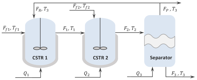
6.1 Process description

In this section, we consider a reactor-separator chemical process that consists of two continuous stirred tank reactors (CSTRs) and one flash tank separator. Based on the physical topology presented in Figure 2, we partition this process into three subsystems, with each subsystem accounting for one vessel.

This chemical process involves two reactions: the first reaction converts reactant AA into desired product BB; the second reaction converts BB into side product CC. The system states include the mass fractions of reactant AA (denoted by xAix_{Ai}, i=1,2,3i=1,2,3), the mass fractions of product BB (denoted by xBix_{Bi}, i=1,2,3i=1,2,3), and the temperatures in three vessels (denoted by TiT_{i}, i=1,2,3i=1,2,3). Among these states, only temperatures TiT_{i} in the three vessels can be measured online. The details of the first-principles nonlinear dynamic model and a more comprehensive description of this chemical process can be found in [15]. The objective is to implement the proposed DMHE approach, where the arrival costs for the local estimators are updated using a recursive method for estimating the nine system states based on the measured outputs TiT_{i}, i=1,2,3i=1,2,3.

Table 1: The initial state x0x_{0} and the initial guess x¯0\bar{x}_{0} for the chemical process.
xA1x_{A1} xB1x_{B1} T1T_{1} (K)(\mathrm{K}) xA2x_{A2} xB2x_{B2} T2T_{2} (K)(\mathrm{K}) xA3x_{A3} xB3x_{B3} T3T_{3} (K)(\mathrm{K})
x0x_{0} 0.1939 0.7404 528.3482 0.2162 0.7190 520.0649 0.0716 0.7373 522.3765
x¯0\bar{x}_{0} 0.2521 0.9625 686.8525 0.2810 0.9346 676.0844 0.0931 0.9585 679.0894

In the simulations, the heat exchange rates considered in this process are Q1=(2.9+1.74Q_{1}=(2.9+1.74 sin(0.06πt))×106kJ/h\sin(0.06\pi t))\times 10^{6}~{}\mathrm{kJ/h}, Q2=(1+0.6sin(0.06πt))Q_{2}=(1+0.6\sin(0.06\pi t)) ×106kJ/h\times 10^{6}~{}\mathrm{kJ/h}, and Q3=(2.9+1.74sin(0.06πt))×106kJ/hQ_{3}=(2.9+1.74\sin(0.06\pi t))\times 10^{6}~{}\mathrm{kJ/h}. The initial state x0x_{0} that is utilized to generate the actual state trajectories of this process is presented in Table 1. All the states are scaled to ensure equal importance is assigned to states of different magnitudes. Unknown process disturbances and measurement noise are generated following a zero-mean Gaussian distribution with a standard deviation of 0.010.01 for process disturbances and 0.050.05 for measurement noise, which are further added to the states and output measurements in the scaled coordinate, respectively.

6.2 Simulation results

Refer to caption
Figure 3: Trajectories of the actual system state and the state estimates provided by the proposed DMHE algorithm for three vessels.
Table 2: Comparison of RMSEs.
Proposed DMHE DMHE-1 DMHE-2
RMSE 0.1384 0.1425 0.2595

The estimation window is N=4N=4. The initial guess for the proposed DMHE is picked as x¯0=1.3×x0\bar{x}_{0}=1.3\times x_{0}, as presented in Table 1. The initial weighting matrices Pi,0P_{i,0}, QiQ_{i}, and RiR_{i}, i𝕀i\in\mathbb{I}, are chosen as Pi,0=0.001×I3P_{i,0}=0.001\times I_{3}, Qi=0.01×I3Q_{i}=0.01\times I_{3}, and R=0.05×I3R=0.05\times I_{3}. We impose constraints on the estimates of xAix_{Ai} and xBix_{Bi}, i=1,2,3i=1,2,3, generated by the proposed DMHE such that they stay within the range of [0,1][0,1], while the estimates of temperatures TiT_{i}, i=1,2,3i=1,2,3, are made positive.

Refer to caption
Figure 4: Trajectories of the actual system state and the state estimates provided by the proposed DMHE algorithm and the DMHE-3 approach for three vessels.

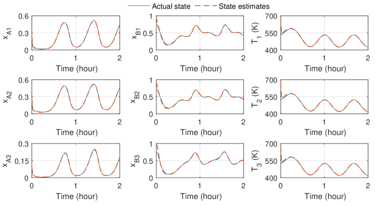
The trajectories of the state estimates given by the proposed DMHE algorithm and the actual states are presented in Figure 3. The proposed DMHE approach provides accurate estimates of the ground truth of all the process states, which demonstrates the robustness of the proposed DMHE approach against unknown disturbances. Additionally, we evaluate and compare the estimation performance of the proposed DMHE approach with two DMHE algorithms of which each local estimator only uses the sensor measurements of the corresponding subsystems: 1) DMHE-1, where the arrival cost is constructed as a weighted squared error between the state estimate and the a priori state prediction, with the weighting matrix determined by a constant matrix; 2) DMHE-2, where the arrival cost is not considered in DMHE algorithm. The constant weighting matrices PiP_{i}, QiQ_{i}, and RR, i=1,2,3i=1,2,3, of DMHE-1, are chosen the same as the initial weighting matrices of the proposed DMHE method. The root mean squared errors (RMSE) for the three DMHE algorithms in the scaled coordinate are shown in Table 2. The proposed DMHE algorithm provides more accurate estimates than the other two methods.

Refer to caption
Figure 5: Trajectories of the estimation error norm of the proposed proposed DMHE algorithm and the DMHE-3 approach.

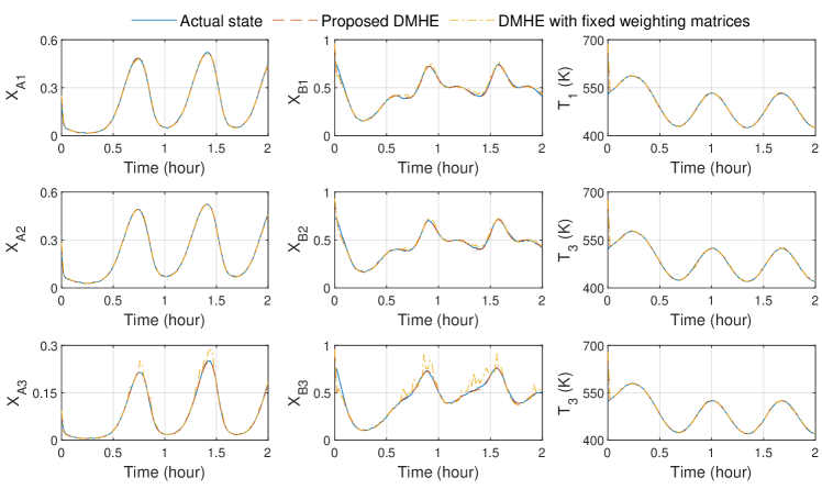
To further illustrate the superiority of employing a recursive approach to approximate and update the arrival costs at each sampling instant, we compare it with DMHE-3, where the arrival costs of local estimators are designed as a weighted squared error between the estimate of state and the initial guess of state, weighted by a constant matrix throughout the simulation period. Different from DMHE-1 in the previous comparison, DMHE-3 incorporates sensor measurements from the interconnected subsystems into the objective function of the local estimator design in the same manner as our proposed DMHE approach. In this comparison, we randomly select the weighting matrices of DMHE-3 without fine-tuning for this process. Specifically, the constant weighting matrices PiP_{i}, QiQ_{i}, and RR for the iith estimator of DMHE-3 are diagonal matrices with the main diagonal elements set to 1, 0.001, and 0.001, respectively. These matrices for DMHE-3 also serve as the initial weighting matrices for our proposed DMHE algorithm. In contrast, the matrix PiP_{i} will be updated following (25) and (75) at every sampling instant when conducting state estimation using our proposed DMHE approach.

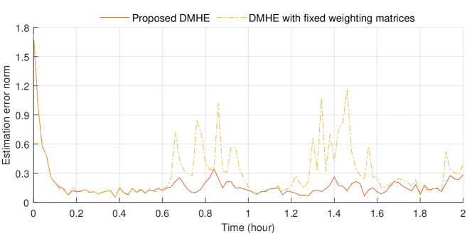
The trajectories of actual states and the estimates provided by both the proposed DMHE algorithm and DMHE-3 are shown in Figure 4, and the corresponding trajectories of the estimation errors are presented in Figure 5. The results demonstrate that the proposed DMHE approach outperforms DMHE-3 overall in terms of estimation accuracy. It is worth mentioning that when constant weighting matrices are employed for DMHE, extensive trial and error analysis is typically needed to fine-tune the weighting matrices for good estimation performance. In contrast, the arrival cost of each local estimator is updated at each sampling instant in our proposed DMHE algorithm, which allows for less accurate initial parameters and is more favorable for implementation.

Remark 1.

Compared with the iterative DMHE approaches in [8, 10, 12] that require iterative executions within each sampling period, our proposed DMHE method offers more efficient computation. This improvement is attributed to the update of the arrival cost at each sampling instant. Our approach employs a recursive method to provide a more accurate approximation of the arrival cost, which not only improves the accuracy of the state estimates but also reduces the computation complexity because the local estimators are only required to be executed once within each sampling period.

Remark 2.

One of the important tuning parameters that affect the trade-off between the estimation accuracy and the computational complexity is the length of the estimation window for the local estimators, denoted by NN. From an application perspective, a larger NN has the potential to enhance the estimation accuracy of the DMHE approach. Meanwhile, increasing NN also leads to increased complexity of the online optimization problems associated with the local estimators, leading to a higher computational burden. Therefore, a good trade-off between the estimation accuracy and the computational complexity should be achieved via appropriately adjusting the window length N.

7 Concluding Remarks

We addressed a partition-based distributed state estimation problem for general nonlinear systems. A recursive approach was introduced to approximate the arrival cost for each MHE-based estimator of the DMHE scheme. A partition-based distributed full-information estimation formulation was employed to derive an analytical expression for the arrival costs of local estimators of the DMHE algorithm in the linear unconstrained context. Based on the derived arrival cost for each local estimator, the proposed DMHE estimator for constrained linear systems was proposed, and the stability of the proposed DMHE scheme for linear systems was proven. Subsequently, through successive linearization of nonlinear subsystem models, the arrival cost design for linear unconstrained systems was extended to the nonlinear context. Accordingly, we proposed a partition-based DMHE algorithm for constrained nonlinear processes. The proposed DMHE method was applied to a simulated chemical process, and the results confirmed its superiority and efficacy.

In the future research, we will investigate the stability of the DMHE approach for nonlinear systems and the development of a robust DMHE algorithm for systems with uncertain model parameters.

Acknowledgment

This research is supported by the Ministry of Education, Singapore, under its Academic Research Fund Tier 1 (RG63/22), and Nanyang Technological University, Singapore (Start-Up Grant).

References

  • [1] P. D. Christofides, R. Scattolini, D. M. de la Peña, J. Liu. Distributed model predictive control: A tutorial review and future research directions. Computers & Chemical Engineering, 51:21–41, 2013.
  • [2] G. Battistelli, L. Chisci. Stability of consensus extended Kalman filter for distributed state estimation. Automatica, 68:169–178, 2016.
  • [3] X. Yin, J. Zeng, J. Liu. Forming distributed state estimation network from decentralized estimators. IEEE Transactions on Control Systems Technology, 27(6):2430–2443, 2018.
  • [4] P. Daoutidis, W. Tang, A. Allman. Decomposition of control and optimization problems by network structure: Concepts, methods, and inspirations from biology. AIChE Journal, 65(10), 2019.
  • [5] W. Tang, A. Allman, D. B. Pourkargar, P. Daoutidis. Optimal decomposition for distributed optimization in nonlinear model predictive control through community detection. Computers & Chemical Engineering, 111:43–54, 2018.
  • [6] S. Chen, Z. Wu, D. Rincon, P. D. Christofides. Machine learning-based distributed model predictive control of nonlinear processes. AIChE Journal, 66(11):e17013, 2020.
  • [7] M. Farina, G. Ferrari-Trecate, R. Scattolini. Moving-horizon partition-based state estimation of large-scale systems. Automatica, 46(5):910–918, 2010.
  • [8] R. Schneider, W. Marquardt. Convergence and stability of a constrained partition-based moving horizon estimator. IEEE Transactions on Automatic Control, 61(5):1316–1321, 2015.
  • [9] R. Schneider. A solution for the partitioning problem in partition-based moving-horizon estimation. IEEE Transactions on Automatic Control, 62(6):3076–3082, 2017.
  • [10] R. Schneider, R. Hannemann-Tamás, W. Marquardt. An iterative partition-based moving horizon estimator with coupled inequality constraints. Automatica, 61:302–307, 2015.
  • [11] X. Yin, B. Huang. Event-triggered distributed moving horizon state estimation of linear systems. IEEE Transactions on Systems, Man, and Cybernetics: Systems, 52(10):6439–6451, 2022.
  • [12] X. Li, S. Bo, Y. Qin, X. Yin. Iterative distributed moving horizon estimation of linear systems with penalties on both system disturbances and noise. Chemical Engineering Research and Design, 194:878–893, 2023.
  • [13] X. Yin, J. Liu. Distributed moving horizon state estimation of two-time-scale nonlinear systems. Automatica, 79:152–161, 2017.
  • [14] M. Farina, G. Ferrari-Trecate, C. Romani, R. Scattolini. Moving horizon estimation for distributed nonlinear systems with application to cascade river reaches. Journal of Process Control, 21(5):767–774, 2011.
  • [15] J. Zhang, J. Liu. Distributed moving horizon state estimation for nonlinear systems with bounded uncertainties. Journal of Process Control, 23(9):1281–1295, 2013.
  • [16] J. Zeng, J. Liu. Distributed moving horizon state estimation: Simultaneously handling communication delays and data losses. Systems & Control Letters, 75:56–68, 2015.
  • [17] C. C. Qu, J. Hahn. Computation of arrival cost for moving horizon estimation via unscented Kalman filtering. Journal of Process Control, 19(2):358–363, 2009.
  • [18] R. López-Negrete, S. C. Patwardhan, L. T. Biegler. Constrained particle filter approach to approximate the arrival cost in moving horizon estimation. Journal of Process Control, 21(6):909–919, 2011.
  • [19] C. V. Rao, J. B. Rawlings, J. H. Lee. Constrained linear state estimation – a moving horizon approach. Automatica, 37(10):1619–1628, 2001.
  • [20] M. Gharbi, C. Ebenbauer. Proximity moving horizon estimation for linear time-varying systems and a Bayesian filtering view. IEEE Conference on Decision and Control, 3208–3213, Nice, France, 2019.
  • [21] C. V. Rao, J. B. Rawlings. Constrained process monitoring: Moving-horizon approach. AIChE Journal, 48(1):97–109, 2002.
  • [22] M. Gharbi, F. Bayer, C. Ebenbauer. Proximity moving horizon estimation for discrete-time nonlinear systems. IEEE Control Systems Letters, 5(6):2090–2095, 2020.
  • [23] X. Li, S. Bo, X. Zhang, Y. Qin, X. Yin. Data‐driven parallel Koopman subsystem modeling and distributed moving horizon state estimation for large‐scale nonlinear processes. AIChE Journal, 70(3):e18326, 2024.
  • [24] X. Li, A. W. K. Law, X. Yin. Partition-based distributed extended Kalman filter for large-scale nonlinear processes with application to chemical and wastewater treatment processes. AIChE Journal, 69(12):e18229, 2023.
  • [25] X. Li, X. Yin. A recursive approach to approximate arrival costs in distributed moving horizon estimation. IFAC Conference on Nonlinear Model Predictive Control, Accepted.
  • [26] P. K. Findeisen. Moving horizon state estimation of discrete time systems. Ph.D. thesis, University of Wisconsin–Madison, 1997.
  • [27] S. Knüfer, M. A. Müller. Nonlinear full information and moving horizon estimation: Robust global asymptotic stability. Automatica, 150:110603, 2023.
  • [28] J. Rawlings, D. Mayne. Postface to model predictive control: Theory and design. Nob Hill Pub, 5:155–158, 2012.
  • [29] H. Henderson, S. Searle. On deriving the inverse of a sum of matrices. SIAM Review, 23(1):53–60, 1981.
  • [30] M. Farina, G. Ferrari-Trecate, R. Scattolini. Moving horizon partition-based state estimation of large-scale systems–Revised version. arXiv:2401.17933, 2024.