Approximating -Median Clustering for Polygonal Curves
Abstract
In 2015, Driemel, Krivošija and Sohler introduced the -median problem for clustering polygonal curves under the Fréchet distance. Given a set of input curves, the problem asks to find median curves of at most vertices each that minimize the sum of Fréchet distances over all input curves to their closest median curve. A major shortcoming of their algorithm is that the input curves are restricted to lie on the real line. In this paper, we present a randomized bicriteria-approximation algorithm that works for polygonal curves in and achieves approximation factor with respect to the clustering costs. The algorithm has worst-case running-time linear in the number of curves, polynomial in the maximum number of vertices per curve, i.e. their complexity, and exponential in , , and , i.e., the failure probability. We achieve this result through a shortcutting lemma, which guarantees the existence of a polygonal curve with similar cost as an optimal median curve of complexity , but of complexity at most , and whose vertices can be computed efficiently. We combine this lemma with the superset-sampling technique by Kumar et al. to derive our clustering result. In doing so, we describe and analyze a generalization of the algorithm by Ackermann et al., which may be of independent interest.
1 Introduction
Since the development of -means – the pioneer of modern computational clustering – the last 65 years have brought a diversity of specialized [31, 7, 20, 6, 13, 19, 32] as well as generalized clustering algorithms [24, 2, 5]. However, in most cases clustering of point sets was studied. Many clustering problems indeed reduce to clustering of point sets, but for sequential data like time-series and trajectories – which arise in the natural sciences, medicine, sports, finance, ecology, audio/speech analysis, handwriting and many more – this is not the case. Hence, we need specialized clustering methods for these purposes, cf. [1, 12, 18, 29, 30].
A promising branch of this active research deals with -center and -median clustering – adaptions of the well-known Euclidean -center and -median clustering. In -center clustering, respective -median clustering, we are given a set of polygonal curves in of complexity (i.e., the number of vertices of the curve) at most each and want to compute centers that minimize the objective function – just as in Euclidean -clustering. In addition, the centers are restricted to have complexity at most each to prevent over-fitting – a problem specific for sequential data. A great benefit of regarding the sequential data as polygonal curves is that we introduce an implicit linear interpolation. This does not require any additional storage space since we only need to store the vertices of the curves, which are the sequences at hand. We compare the polygonal curves by their Fréchet distance, that is a continuous distance measure which takes the entire course of the curves into account, not only the pairwise distances among their vertices. Therefore, irregular sampled sequences are automatically handled by the interpolation, which is desirable in many cases. Moreover, Buchin et al. [10] showed, by using heuristics, that the -clustering objectives yield promising results on trajectory data.
This branch of research formed only recently, about twenty years after Alt and Godau developed an algorithm to compute the Fréchet distance between polygonal curves [4]. Several papers have since studied this type of clustering [15, 9, 10, 11, 26]. However, all of these clustering algorithms, except the approximation-schemes for polygonal curves in [15] and the heuristics in [10], choose a -subset of the input as centers. (This is also often called discrete clustering.) This -subset is later simplified, or all input-curves are simplified before choosing a -subset. Either way, using these techniques one cannot achieve an approximation factor of less than . This is because there need not be an input curve with distance to its median which is less than the average distance of a curve to its median.
Driemel et al. [15], who were the first to study clustering of polygonal curves under the Fréchet distance in this setting, already overcame this problem in one dimension by defining and analyzing -signatures, which are succinct representations of classes of curves that allow synthetic center-curves to be constructed. However, it seems that -signatures are only applicable in . Here, we extend their work and obtain the first randomized bicriteria approximation algorithm for -median clustering of polygonal curves in .
1.1 Related Work
Driemel et al. [15] introduced the -center and -median objectives and developed the first approximation-schemes for these objectives, for curves in . Furthermore, they proved that -center as well as -median clustering is NP-hard, where is a part of the input and is fixed. Also, they showed that the doubling dimension of the metric space of polygonal curves under the Fréchet distance is unbounded, even when the complexity of the curves is bounded.
Following this work, Buchin et al. [9] developed a constant-factor approximation algorithm for -center clustering in . Furthermore, they provide improved results on the hardness of approximating -center clustering under the Fréchet distance: the -center problem is NP-hard to approximate within a factor of for curves in and within a factor of for curves in , where , in both cases even if . Furthermore, for the -median variant, Buchin et al. [11] proved NP-hardness using a similar reduction. Again, the hardness holds even if . Also, they provided -approximation algorithms for -center, as well as -median clustering, under the discrete Fréchet distance. Nath and Taylor [28] give improved algorithms for -approximation of -median clustering under discrete Fréchet and Hausdorff distance. Recently, Meintrup et al. [26] introduced a practical -approximation algorithm for discrete -median clustering under the Fréchet distance, when the input adheres to a certain natural assumption, i.e., the presence of a certain number of outliers.
Our algorithms build upon the clustering algorithm of Kumar et al. [25], which was later extended by Ackermann et al. [2]. This algorithm is a recursive approximation scheme, that employs two phases in each call. In the so-called candidate phase it computes candidates by taking a sample from the input set and running an algorithm on each subset of of a certain size. Which algorithm to use depends on the metric at hand. The idea behind this is simple: if contains a cluster that takes a constant fraction of its size, then a constant fraction of is from with high probability. By brute-force enumeration of all subsets of , we find this subset and if is taken uniformly and independently at random from then is a uniform and independent sample from . Ackermann et al. proved for various metric and non-metric distance measures, that can be used for computing candidates that contain a -approximate median for with high probability. The algorithm recursively calls itself for each candidate to eventually evaluate these together with the candidates for the remaining clusters.
The second phase of the algorithm is the so-called pruning phase, where it partitions its input according to the candidates at hand into two sets of equal size: one with the smaller distances to the candidates and one with the larger distances to the candidates. It then recursively calls itself with the second set as input. The idea behind this is that small clusters now become large enough to find candidates for these. Furthermore, the partitioning yields a provably small error. Finally it returns the set of candidates that together evaluated best.
1.2 Our Contributions
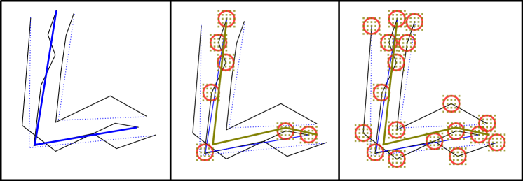
We present several algorithms for approximating -median clustering of polygonal curves under the Fréchet distance, see Fig. 1 for an illustration of the operation principles of our algorithms. While the first one, Algorithm 1, yields only a coarse approximation (factor 34), it is suitable as plugin for the following two algorithms, Algorithms 2 and 4, due to its asymptotically fast running-time. These algorithms yield a better approximation (factor , respectively ). Additionally, Algorithms 2 and 4 are not only able to yield an approximation for the input set , but for a cluster , that takes a constant fraction of . We would like to use these as plugins to the -approximation algorithm for -median clustering by Ackermann et al. [2], but that would require our algorithms to comply with the sampling properties. For an input set the weak sampling property expresses that a constant-size set of candidates can be computed, that contains a -approximate median for with high probability, by taking a constant-size uniform and independent sample of . Further, the running-time for computing the candidates depends only on the size of the sample, the size of the candidate set and the failure probability parameter. The strong sampling property is defined similarly, but instead of a candidate set, an approximate median can be computed directly and the running-time may only depend on the size of the sample. In our algorithms, the running-time for computing the candidate set depends on which is a parameter of the input. Additionally, our first algorithm for computing candidates, which contain a -approximate -median with high probability, does not achieve the required approximation-factor of . However, looking into the analysis of Ackermann et al., any algorithm for computing candidates, with some guaranteed approximation-factor, can be used in the recursive approximation-scheme. Therefore, we decided to generalize the -median clustering algorithm of Ackermann et al. [2].
Nath and Taylor [28] use a similar approach, but they developed yet another way to compute candidates: they define and analyze -coverability, which is a generalization of the notion of doubling dimension and indeed, for the discrete Fréchet distance the proof builds upon the doubling dimension of points in . However, the doubling dimension of polygonal curves under the Fréchet distance is unbounded, even when the complexities of the curves are bounded and it is an open question whether -coverability holds for the continuous Fréchet distance.
We circumvent this by taking a different approach using the idea of shortcutting. It is well-known that shortcutting a polygonal curve (that is, replacing a subcurve by the line segment connecting its endpoints) does not increase its Fréchet distance to a line segment. This idea has been used before for a variety of Fréchet-distance related problems [3, 15, 14, 8]. Specifically, we introduce two new shortcutting lemmata. These lemmata guarantee the existence of good approximate medians, with complexity at most and whose vertices can be computed efficiently. The first one enables us to return candidates, which contain a -approximate median for a cluster inside the input, that takes a constant fraction of the input, w.h.p., and we call it simple shortcutting. The second one enables us to return candidates, which contain a -approximate median for a cluster inside the input, that takes a constant fraction of the input, w.h.p., and we call it advanced shortcutting. All in all, we obtain as main result, following from Corollary 7.5:
Theorem 1.1.
Given a set of polygonal curves in , of complexity at most each, parameter values and , and constants , there exists an algorithm, which computes a set of polygonal curves, each of complexity at most , such that with probability at least , it holds that
where is an optimal -median solution for under the Fréchet distance .
The algorithm has worst-case running-time linear in , polynomial in and exponential in and .
1.3 Organization
The paper is organized as follows. First we present a simple and fast -approximation algorithm for -median clustering. Then, we present the -approximation algorithm for -median clustering of a cluster inside the input, that takes a constant fraction of the input, which builds upon simple shortcutting and the -approximation algorithm. Then, we present a more practical modification of the -approximation algorithm, which achieves a -approximation for -median clustering. Following this, we present the similar but more involved -approximation algorithm for -median clustering of a cluster inside the input, that takes a constant fraction of the input, which builds upon the advanced shortcutting and the -approximation algorithm. Finally we present the generalized recursive -median approximation-scheme, which leads to our main result.
2 Preliminaries
Here we introduce all necessary definitions. In the following is an arbitrary constant. By we denote the Euclidean norm and for and we denote by the closed ball of radius with center . By we denote the symmetric group of degree . We give a standard definition of grids:
Definition 2.1 (grid).
Given a number , for we define by the -grid-point of . Let be a subset of . The grid of cell width that covers is the set .
Such a grid partitions the set into cubic regions and for each and we have that . We give a standard definition of polygonal curves:
Definition 2.2 (polygonal curve).
A (parameterized) curve is a continuous mapping . A curve is polygonal, iff there exist , no three consecutive on a line, called ’s vertices and with , and , called ’s instants, such that connects every two contiguous vertices by a line segment.
We call the line segments the edges of and the complexity of , denoted by . Sometimes we will argue about a sub-curve of a given curve . We will then refer to by restricting the domain of , denoted by , where .
Definition 2.3 (Fréchet distance).
Let denote the set of all continuous bijections with and , which we call reparameterizations. The Fréchet distance between curves and is defined as
Sometimes, given two curves , we will refer to an as matching between and .
Note that there must not exist a matching , such that . This is due to the fact that in some cases a matching realizing the Fréchet distance would need to match multiple points on to a single point on , which is not possible since matchings need to be bijections, but the can get matched arbitrarily close to , realizing in the limit, which we formalize in the following lemma:
Lemma 2.4.
Let be curves. Let . There exists a sequence in , such that .
Proof.
Define with image . Per definition, we have .
For any non-empty subset of that is bounded from below and for every it holds that there exists an with , by definition of the infimum. Since and exists, for every there exists an with .
Now, let be a zero sequence. For every there exists an with , thus .
Let be the preimage of . Since is a function, for each . Now, for , let be an arbitrary element from . By definition it holds that
which proves the claim. ∎
Now we introduce the classes of curves we are interested in.
Definition 2.5 (polygonal curve classes).
For , we define by the equivalence class of polygonal curves (where two curves are equivalent, iff they can be made identical by a reparameterization) in ambient space . For we define by the subclass of polygonal curves of complexity at most .
Simplification is a fundamental problem related to curves and which appears as sub-problem in our algorithms.
Definition 2.6 (minimum-error -simplification).
For a polygonal curve we denote by an -approximate minimum-error -simplification of , i.e., a curve with for all .
Now we define the -median clustering problem for polygonal curves.
Definition 2.7 (-median clustering).
The -median clustering problem is defined as follows, where are fixed (constant) parameters of the problem: given a finite and non-empty set of polygonal curves, compute a set of curves , such that is minimal.
We call the objective function and we often write as shorthand for . The following theorem of Indyk [23] is useful for evaluating the cost of a curve at hand.
Theorem 2.8.
[23, Theorem 31] Let and be a set of polygonal curves. Further let be a non-empty sample, drawn uniformly and independently at random from , with replacement. For with it holds that .
The following concentration bound also applies to independent Bernoulli trials, which are a special case of Poisson trials where each trial has same probability of success. Kumar et al. [25] use this to bound the probability that a subset of an independent and uniform sample from a set is entirely contained in a subset of . They call it superset-sampling.
Lemma 2.9 (Chernoff bound for independent Poisson trials).
[27, Theorem 4.5] Let be independent Poisson trials. For it holds that
3 Simple and Fast -Approximation for -Median
Here, we present Algorithm 1, a -approximation algorithm for -median clustering, which is based on the following facts: we can obtain a -approximate solution to the -median for a given set of polygonal curves in terms of objective value, i.e., we obtain one of the at least input curves that are within distance to an optimal -median for , w.h.p., by uniformly and independently sampling a sufficient number of curves from . There are at least of these curves by an averaging argument. These curves have cost up to by the triangle-inequality. The sample has size depending only on a parameter determining the failure probability and we can improve on running-time even more by using Theorem 2.8 and evaluate the cost of each curve in the sample of candidates against another sample of similar size instead of against the complete input. Though, we have to accept an approximation factor of (if we set in Theorem 2.8). That is indeed acceptable, since we only obtain an approximate solution in terms of objective value and completely ignore the bound on the number of vertices of the center curve, which is a disadvantage of this approach and results in the lower bound of not necessarily holding (if ). To fix this, we simplify the candidate curve that evaluated best against the second sample, using an efficient minimum-error -simplification approximation algorithm, which downgrades the approximation factor to , where is the approximation factor of the minimum-error -simplification.
However, Algorithm 1 is very fast in terms of the input size. Indeed, it has worst-case running-time independent of and sub-quartic in . Now, Algorithm 1 has the purpose to provide us an approximate median for a given set of polygonal curves: the bi-criteria approximation algorithms (Algorithms 2 and 4), which we present afterwards and which are capable of generating center curves with up to vertices, need an approximate median (and the approximation factor) to bound the optimal objective value. Furthermore, there is a case where Algorithms 2 and 4 may fail to provide a good approximation, but it can be proven that the result of Algorithm 1 is then a very good approximation, which can be used instead.
Next, we prove the quality of approximation of Algorithm 1.
Theorem 3.1.
Given a parameter and a set of polygonal curves, Algorithm 1 returns with probability at least a polygonal curve , such that , where is an optimal -median for and is the approximation-factor of the utilized minimum-error -simplification approximation algorithm.
Proof.
First, we know that , for each .
Now, there are at least curves in that are within distance at most to . Otherwise the cost of the remaining curves would exceed , which is a contradiction. Hence each has probability at least to be within distance to .
Since the elements of are sampled independently we conclude that the probability that every has distance to greater than is at most .
Now, assume there is a with . We do not want any with to have . Using Theorem 2.8 we conclude that this happens with probability at most
for each .
Using a union bound over all bad events, we conclude that with probability at least , Algorithm 1 samples a curve , with and returns the simplification of a curve , with . The triangle-inequality yields
which is equivalent to
Hence, we have
The lower bound follows from the fact that the returned curve has vertices and that has minimum cost among all curves with vertices. ∎
The following lemma enables us to obtain a concrete approximation-factor and worst-case running-time of Algorithm 1.
Lemma 3.2 (Buchin et al. [9, Lemma 7.1]).
Given a curve , a -approximate minimum-error -simplification can be computed in time.
The simplification algorithm used for obtaining this statement is a combination of the algorithm by Imai and Iri [22] and the algorithm by Alt and Godau [4]. Combining Theorem 3.1 and Lemma 3.2, we obtain the following corollary.
Corollary 3.3.
Given a parameter and a set of polygonal curves, Algorithm 1 returns with probability at least a polygonal curve , such that , where is an optimal -median for , in time , when the algorithms by Imai and Iri [22] and Alt and Godau [4] are combined for -simplification.
Proof.
We use Lemma 3.2 together with Theorem 3.1, which yields an approximation factor of . Now, drawing the first sample takes time . Drawing the second sample also takes time and evaluating the samples against each other takes time . Simplifying one of the curves that evaluates best takes time . We conclude that Algorithm 1 has running-time . ∎
4 -Approximation for -Median by Simple Shortcutting
Here, we present Algorithm 2, which returns candidates, containing a -approximate -median of complexity at most , for a cluster contained in the input, that takes a constant fraction of the input, w.h.p. Algorithm 2 can be used as plugin in our generalized version (Algorithm 5, Section 7) of the algorithm by Ackermann et al. [2].
In contrast to Nath and Taylor [28] we cannot use the property, that the vertices of a median must be found in the balls of radius , centered at ’s vertices, where is an optimal -median for a given input , which is an element of. This is an immediate consequence of using the continuous Fréchet distance.
We circumvent this by proving the following shortcutting lemmata. We start with the simplest, which states that we can indeed search the aforementioned balls, if we accept a resulting curve of complexity at most . See Fig. 2 for a visualization.
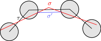
Lemma 4.1 (shortcutting using a single polygonal curve).
Let be polygonal curves. Let be the vertices of and let . There exists a polygonal curve with every vertex contained in at least one of , and .
Proof.
Let be the vertices of . Further, let and be the instants of and , respectively. Also, for (recall that is the set of all continuous bijections with and ), let be the distance realized by . We know from Lemma 2.4 that there exists a sequence in , such that .
Now, fix an arbitrary and assume there is a vertex of , with instant , that is not contained in any of . Let be the maximum of , such that . So is matched to by . We modify in such a way, that is replaced by two new vertices that are elements of and , respectively.
Namely, let be the maximum of , such that and let be the minimum of , such that . These are the instants when leaves before visiting and enters after visiting , respectively. Let be the piecewise defined curve, defined just like on and , but on it connects and with the line segment .
We know that and . Note that and since and are closest points to on that have distance to and , respectively, by definition. Therefore, has no vertices between the instants and . Now, can be used to match to and to with distance at most . Since and are just line segments, they can be matched to each other with distance at most . We conclude that .
Because this modification works for every , we have for every . Thus, .
Now, to prove the claim, for every we apply this modification to and successively to every other vertex of the resulting curve , not contained in one of the balls, until every vertex of is contained in a ball. Note that the modification is repeated at most times for every , since the start and end vertex of must be contained in and , respectively. Therefore, the number of vertices of every can be bounded by since every other vertex must not lie in a ball and for each such vertex one new vertex is created. Thus, . ∎
We now present Algorithm 2, which works similar as Algorithm 1, but uses shortcutting instead of simplification. As a consequence, we can achieve an approximation factor of , instead of a factor of , where is the approximation factor of the simplifiaction algorithm used in Algorithm 1. To achieve an approximation-factor of using simplification, one would need to compute the optimal minimum-error -simplifications of the input curves and to the best of our knowledge, there is no such algorithm for the continuous Fréchet distance.
In contrast to Algorithm 1, Algorithm 2 utilizes the superset-sampling technique by Kumar et al. [25], i.e., the concentration bound in Lemma 2.9, to obtain an approximate -median for a cluster contained in the input , that takes a constant fraction of . Therefore, it has running-time exponential in the size of the sample . A further difference is that we need an upper and a lower bound on the cost of an optimal -median for , to properly set up the grids we use for shortcutting. The lower bound can be obtained by simple estimation, using Markov’s inequality. For the upper bound we utilize a case distinction, which guarantees us that if we fail to obtain an upper bound on the optimal cost, the result of Algorithm 1 then is a good approximation (factor ) and can be used instead of a best curve obtained by shortcutting.
Algorithm 2 has several parameters: determines the size (in terms of a fraction of the input) of the smallest cluster inside the input for which an approximate median can be computed, determines the probability of failure of the algorithm and determines the approximation factor.
We prove the quality of approximation of Algorithm 2.
Theorem 4.2.
Given three parameters , and a set of polygonal curves, with probability at least the set of candidates that Algorithm 2 returns contains a -approximate -median with up to vertices for any , if .
Proof.
We assume that . Let be the number of sampled curves in that are elements of . Clearly, . Also is the sum of independent Bernoulli trials. A Chernoff bound (cf. Lemma 2.9) yields:
In other words, with probability at most no subset , of cardinality at least , is a subset of . We condition the rest of the proof on the contrary event, denoted by , namely, that there is a subset with and . Note that is then a uniform and independent sample of .
Now, let be an optimal -median for . The expected distance between and is
By linearity we have . Markov’s inequality yields:
We conclude that with probability at most we have .
Using Markov’s inequality again, for every we have
therefore by independence
Hence, with probability at most there is no with . Also, with probability at most Algorithm 1 fails to compute a -approximate -median for , cf. Corollary 3.3.
Using a union bound over these bad events, we conclude that with probability at least all of the following events occur simultaneously:
-
•
There is a subset of cardinality at least that is a uniform and independent sample of ,
-
•
there is a curve with ,
-
•
Algorithm 1 computes a polygonal curve with , where is an optimal -median for ,
-
•
and it holds that .
Since is an optimal -median for we get the following from the last two items:
We now distinguish between two cases:
Case 1:
The triangle-inequality yields
As a consequence, .
Now, let be the vertices of . By Lemma 4.1 there exists a polygonal curve with up to vertices, every vertex contained in one of and .
In the set of candidates, that Algorithm 2 returns, a curve with up to vertices from the union of the grid covers and distance at most between every corresponding pair of vertices of and is contained. We conclude that .
We can now bound the cost of as follows:
Case 2:
The cost of can easily be bounded:
The claim follows by rescaling by . ∎
Next we analyse the worst-case running-time of Algorithm 2 and the number of candidates it returns.
Theorem 4.3.
Algorithm 2 has running-time and returns number of candidates .
Proof.
The sample has size and sampling it takes time . Let . The for-loop runs
times. In each iteration, we run Algorithm 1, taking time (cf. Corollary 3.3), we compute the cost of the returned curve with respect to , taking time , and per curve in we build up to grids of size
each. For each curve , Algorithm 2 then enumerates all combinations of points from these up to grids, resulting in
candidates per , per iteration of the for-loop. Thus, Algorithm 2 computes candidates per iteration of the for-loop and enumeration also takes time per iteration of the for-loop.
All in all, we have running-time and number of candidates . ∎
5 More Practical Approximation for -Median by Simple Shortcutting
The following algorithm is a modification of Algorithm 2. It is more practical since it needs to cover only up to (small) balls, using grids. Unfortunately, it is not compatible with the superset-sampling technique and can therefore not be used as plugin in Algorithm 5.
We prove the quality of approximation of Algorithm 3.
Theorem 5.1.
Given two parameters and a set of polygonal curves, with probability at least Algorithm 3 returns a -approximate -median for with up to vertices.
Proof.
Let be an optimal -median for .
The expected distance between and is
Now using Markov’s inequality, for every we have
therefore by independence
Hence, with probability at most there is no with . Now, assume there is a with . We do not want any with to have . Using Theorem 2.8, we conclude that this happens with probability at most
for each . Also, with probability at most Algorithm 1 fails to compute a -approximate -median for , cf. Corollary 3.3.
Using a union bound over these bad events, we conclude that with probability at least , Algorithm 3 samples a curve with and Algorithm 1 computes a -approximate -median for , i.e., . Let be the vertices of . By Lemma 4.1 there exists a polygonal curve with up to vertices, every vertex contained in one of and . Using the triangle-inequality yields
which is equivalent to
Hence, we have .
In the last step, Algorithm 3 returns a curve from the set of all curves with up to vertices from , the union of the grid covers, that evaluates best. We can assume that has distance at most between every corresponding pair of vertices of and . We conclude that .
We can now bound the cost of as follows:
The claim follows by rescaling by . ∎
We analyse the worst-case running-time of Algorithm 3.
Theorem 5.2.
Algorithm 3 has running-time .
Proof.
Algorithm 1 has running-time . The sample has size and the sample has size . Evaluating each curve of against takes time , using the algorithm of Alt and Godau [4] to compute the distances.
Now, has up to vertices and every grid consists of points. Therefore, we have points in and Algorithm 3 enumerates all combinations of points from taking time . Afterwards, these candidates are evaluated, which takes time per candidate using the algorithm of Alt and Godau [4] to compute the distances. All in all, we then have running-time . ∎
6 -Approximation for -Median by Advanced Shortcutting
Now we present Algorithm 4, which returns candidates, containing a -approximate -median of complexity at most , for a cluster contained in the input, that takes a constant fraction of the input, w.h.p. Before we present the algorithm, we present our second shortcutting lemma. Here, we do not introduce shortcuts with respect to a single curve, but with respect to several curves: by introducing shortcuts with respect to well-chosen curves from the given set of polygonal curves, for a given , we preserve the distances to at least curves from . In this context well-chosen means that there exists a certain number of subsets of , of each we have to pick a curve for shortcutting. This will enable the high quality of approximation of Algorithm 4 and we formalize this in the following lemma.
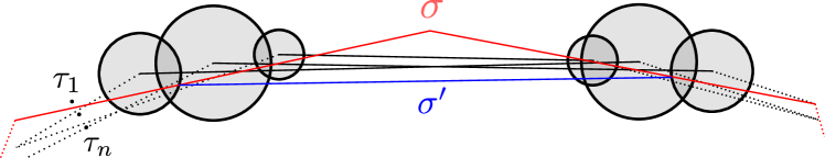
Lemma 6.1 (shortcutting using a set of polygonal curves).
Let be a polygonal curve with vertices and be a set of polygonal curves. For , let and for , let be the th vertex of .
For any there are subsets of curves each (not necessarily disjoint) such that for every subset containing at least one curve out of each , a polygonal curve exists with every vertex contained in
for each and .
The idea is the following, see Fig. 3 for a visualization. One can argue that every vertex of not contained in any of the balls centered at the vertices of the curves in (and of radius according to their distance to ) can be shortcut by connecting the last point before (in terms of the parameter of ) contained in one ball and first point after contained in one ball. This does not increase the Fréchet distances between and the , because only matchings among line segments are affected by this modification. Furthermore, most distances are preserved when we do not actually use the last and first ball before and after , but one of the balls before and one of the balls after , which is the key of the following proof.
Proof of Lemma 6.1.
For the sake of simplicity, we assume that is integral. Let . For , let be the vertices of with instants and let be the vertices of with instants . Also, for (recall that is the set of all continuous bijections with and ) and , let be the distance realized by with respect to . We know from Lemma 2.4 that for each there exists a sequence in , such that .
In the following, given arbitrary , we describe how to modify , such that its vertices can be found in the balls around the vertices of the , of radii determined by . Later we will argue that this modification can be applied using the , for each , in particular.
Now, fix arbitrary and for an arbitrary , fix the vertex of with instant . For , let be the maximum of , such that . Namely, is matched to a point on the line segment , respectively, by .
For , let be the maximum of , such that and let be the minimum of , such that . These are the instants when visits before or when visiting and visits when or after visiting , respectively. Furthermore, there is a permutation of the index set , such that
| (I) |
Also, there is a permutation of the index set , such that
| (II) |
Additionally, for each we have
| (III) |
and
| (IV) |
because and are closest points to on that have distance at most to and , respectively, by definition. We will now use Eqs. I, II, III and IV to prove that an advanced shortcut only affects matchings among line segments and hence we can easily bound the resulting distances for at least of the curves.
Let
is the set of the last curves whose balls are visited by , before or when visits . Similarly, is the set of the first curves whose balls are visited by , when or immediately after visited . We now modify , such that is replaced by two new vertices that are elements of at least one , for a , respectively for a , and , each.
Let be the piecewise defined curve, defined just like on and for arbitrary and , but on it connects and with the line segment
We now argue that for all the Fréchet distance between and is upper bounded by . First, note that by definition are strictly increasing functions, since they are continuous bijections that map to and to . As immediate consequence, we have that
| (V) |
for each and
| (VI) |
for each , using Eqs. I, II, III and IV. Therefore, each has no vertex between the instants and . We also know that for each
| (VII) |
and
| (VIII) |
Let , and . Also, for , let , and . Now, for each we use to match to and to with distance at most . Since and are just line segments by Eqs. V and VI, they can be matched to each other with distance at most
Because this modification works for every , we conclude that for every and . Thus for each .
Now, to prove the claim, for each combination , we apply this modification to and successively to every other vertex of the resulting curve , except and , since these must be elements of and , respectively, for each , by definition of the Fréchet distance.
Since the modification is repeated at most times for each combination , we conclude that the number of vertices of each can be bounded by .
are therefore all the and for , when . Note that every and is determined by the visiting order of the balls and since their radii converge, these sets do too. ∎
We now present Algorithm 4, which is nearly identical to Algorithm 2 but uses the advanced shortcutting lemma. Furthermore, like Algorithm 2, it can be used as plugin in the recursive -median approximation-scheme (Algorithm 5) that we present in Section 7.
We prove the quality of approximation of Algorithm 4.
Theorem 6.2.
Given three parameters , , and a set of polygonal curves, with probability at least the set of candidates that Algorithm 4 returns contains a -approximate -median with up to vertices for any , if .
In the following proof we make use of a case distinction developed by Nath and Taylor [28, Proof of Theorem 10], which is a key ingredient to enable the -approximation, though the domain of has to be restricted to .
Proof of Theorem 6.2.
We assume that . Let be the number of sampled curves in that are elements of . Clearly, . Also is the sum of independent Bernoulli trials. A Chernoff bound (cf. Lemma 2.9) yields:
In other words, with probability at most no subset , of cardinality at least , is a subset of . We condition the rest of the proof on the contrary event, denoted by , namely, that there is a subset with and . Note that is then a uniform and independent sample of .
Now, let be an optimal -median for . The expected distance between and is
By linearity we have . Markov’s inequality yields:
We conclude that with probability at most we have .
Now, from Lemma 6.1 we know that there are subsets , of cardinality each and which are not necessarily disjoint, such that for every set that contains at least one curve for each , there exists a curve which has all of its vertices contained in
and for at least curves it holds that .
There are up to curves with distance to at least . Otherwise the cost of these curves would exceed , which is a contradiction. Later we will prove that each ball we cover has radius at most . Therefore, for each we have to ignore up to half of the curves , since we do not cover the balls of radius centered at their vertices. For each and we now have
Therefore, by independence, for each the probability that no is an element of and has distance to at most is at most . Also, with probability at most Algorithm 1 fails to compute a -approximate -median for , cf. Corollary 3.3.
Using a union bound over these bad events, we conclude that with probability at least all of the following events occur simultaneously:
-
1.
There is a subset of cardinality at least that is a uniform and independent sample of ,
-
2.
for each , contains at least one curve from with distance to up to ,
-
3.
Algorithm 1 computes a polygonal curve with , where is an optimal -median for ,
-
4.
and it holds that .
Let , and . First, note that , otherwise , which is a contradiction, and therefore . We now distinguish two cases:
Case 1:
We have , hence for each . Using independence we conclude that with probability at most
no has distance to greater than . Using a union bound again, we conclude that with probability at least Items 1, 2, 3 and 4 occur simultaneously and at least one has distance to greater than , hence and thus we indeed cover the balls of radius at most .
In the last step, Algorithm 4 returns a set of all curves with up to vertices from the grids, that contains one curve, denoted by with same number of vertices as (recall that this is the curve guaranteed from Lemma 6.1) and distance at most between every corresponding pair of vertices of and . We conclude that . Also, recall that for . Further, contains at least curves with distance at most to , otherwise the cost of the remaining curves would exceed , which is a contradiction, and since there is at least one curve with by the pigeonhole principle. We can now bound the cost of as follows:
Case 2:
Again, we distinguish two cases:
Case 2.1:
We can easily bound the cost of :
Case 2.2:
Recall that . We have
Hence, . Assume we assign all curves to instead of to . For we now have decrease in cost , which can be bounded as follows:
For we have an increase in cost . Let the overall increase in cost be denoted by , which can be bounded as follows:
By the fact that for our choice of , we conclude that , which is a contradiction because is an optimal -median for . Therefore, case 2.2 cannot occur. Rescaling by proves the claim. ∎
We analyse the worst-case running-time of Algorithm 4 and the number of candidates it returns.
Theorem 6.3.
Algorithm 4 has running-time and returns number of candidates .
Proof.
The sample has size and sampling it takes time . Let . The for-loop runs
times. In each iteration, we run Algorithm 1, taking time (cf. Corollary 3.3), we compute the cost of the returned curve with respect to , taking time , and per curve in we build up to grids of size
each. Algorithm 4 then enumerates all combinations of points from up to grids, resulting in
candidates per iteration of the for-loop. Thus, Algorithm 4 computes candidates per iteration of the for-loop and enumeration also takes time per iteration of the for-loop.
All in all, we have running-time and number of candidates . ∎
7 -Approximation for -Median
We generalize the algorithm of Ackermann et al. [2] in the following way: instead of drawing a uniform sample and running a problem-specific algorithm on this sample in the candidate phase, we only run a problem-specific “plugin”-algorithm in the candidate phase, thus dropping the framework around the sampling property. We think that the problem-specific algorithms used in [2] do not fulfill the role of a plugin, since parts of the problem-specific operations, e.g. the uniform sampling, remain in the main algorithm. Here, we separate the problem-specific operations from the main algorithm: any algorithm can serve as plugin, if it is able to return candidates for a cluster that takes a constant fraction of the input, where the fraction is an input-parameter of the algorithm and some approximation factor is guaranteed (w.h.p.). The calls to the candidate-finder plugin do not even need to be independent (stochastically), allowing adaptive algorithms.
Now, let be an arbitrary space, where is any non-empty (ground-)set and is a distance function (not necessarily a metric). We introduce a generalized definition of -median clustering. Let the medians be restricted to come from a predefined subset .
Definition 7.1 (generalized -median).
The generalized -median clustering problem is defined as follows, where is a fixed (constant) parameter of the problem: given a finite and non-empty set , compute a set of elements from , such that is minimal.
The following algorithm, Algorithm 5, can approximate every -median problem compatible with Definition 7.1, when provided with such a problem-specific plugin-algorithm for computing candidates. In particular, it can approximate the -median problem for polygonal curves under the Fréchet distance, when provided with Algorithm 2 or Algorithm 4. Then, we have , and . Note that the algorithm computes a bicriteria approximation, that is, the solution is approximated in terms of the cost and the number of vertices of the center curves, i.e., the centers come from .
Algorithm 5 has several parameters. The first parameter is the set of centers found yet and is the number of centers yet to be found. The following parameters concern only the plugin-algorithm used within the algorithm: determines the size (in terms of a fraction of the input) of the smallest cluster for which an approximate median can be computed, determines the probability of failure of the plugin-algorithm and determines the approximation factor of the plugin-algorithm.
Algorithm 5 works as follows: If it has already computed some centers (and there are still centers to compute) it does pruning: some clusters might be too small for the plugin-algorithm to compute approximate medians for them. Algorithm 5 then calls itself recursively with only half of the input: the elements with larger distances to the centers yet found. This way the small clusters will eventually take a larger fraction of the input and can be found in the candidate phase. In this phase Algorithm 5 calls its plugin and for each candidate that the plugin returned, it calls itself recursively: adding the candidate at hand to the set of centers yet found and decrementing by one. Eventually, all combinations of computed candidates are evaluated against the original input and the centers that together evaluated best are returned.
The quality of approximation and worst-case running-time of Algorithm 5 is stated in the following two theorems, which we prove further below. The proofs are adaptations of corresponding proofs in [2]. We provide them for the sake of completeness.
Theorem 7.2.
Let , and -Median-Candidates be an algorithm that, given three parameters , and a set , returns with probability at least an -approximate -median for any , if .
Algorithm 5 called with parameters , where and , returns with probability at least a set with , where is an optimal set of medians for .
Theorem 7.3.
Let denote the worst-case running-time of -Median-Candidates for an arbitrary input-set with and let denote the maximum number of candidates it returns. Also, let denote the worst-case running-time needed to compute for an input element and a candidate.
If and are non-decreasing in , Algorithm 5 has running-time .
Now we state our main results, which follow from Theorems 4.2 and 4.3, respectively Theorems 6.2 and 6.3, and Theorems 7.2 and 7.3.
Corollary 7.4.
Given two parameters and a set of polygonal curves, Algorithm 5 endowed with Algorithm 2 as -Median-Candidates and run with parameters returns with probability at least a set that is a -approximate solution to the -median for . Algorithm 5 then has running-time .
Corollary 7.5.
Given two parameters and a set of polygonal curves, Algorithm 5 endowed with Algorithm 4 as -Median-Candidates and run with parameters returns with probability at least a set that is a -approximate solution to the -median for . Algorithm 5 then has running-time .
The following proof is an adaption of [2, Theorem 2.2 - Theorem 2.5].
Proof of Theorem 7.2.
For , the claim trivially holds. We now distinguish two cases. In the first case the principle of the proof is presented in all its detail. In the second case we only show how to generalize the first case to .
Case 1:
Let be an optimal set of medians for with clusters and , respectively, that form a partition of . For the sake of simplicity, assume that is a power of and w.l.o.g. assume that . Let be the set of candidates returned by -Median-Candidates in the initial call. With probability at least , there is a with . We distinguish two cases:
Case 1.1:
There exists a recursive call with parameters and .
First, we assume that is the maximum cardinality input with , occurring in a recursive call of the algorithm. Let be the set of candidates returned by -Median-Candidates in this call. With probability at least , there is a with , where is an optimal median for .
Let be the set of elements of removed in the , , pruning phases between obtaining and . Without loss of generality we assume that . For , let be the elements removed in the th (in the order of the recursive calls occurring) pruning phase. Note that the are pairwise disjoint, we have that and . Since , we have
| (I) |
Our aim is now to prove that the number of elements wrongly assigned to , i.e., , is small and further, that their cost is a fraction of the cost of the elements correctly assigned to , i.e., .
We define and for we define . The are the elements remaining after the th pruning phase. Note that by definition . Since is the maximum cardinality input, with , we have that for all . Also, for each we have , therefore
| (II) |
and as immediate consequence
| (III) |
This tells us that mainly the elements of are removed in the pruning phase and only very few elements of . By definition, we have for all , and that , hence
Combining this inequality with Eqs. II and III we obtain for :
| (IV) |
We still need such a bound for . Since and also we can use Eq. II to obtain:
| (V) |
Also, we have for all and that by definition, thus
We combine this inequality with Eq. II and Eq. V and obtain:
| (VI) |
We are now ready to bound the cost of the elements of wrongly assigned to . Combining Eq. IV and Eq. VI yields:
Here, the last inequality holds, because and are pairwise disjoint. Also, we have
Finally, using Eq. I and a union bound, with probability at least the following holds:
Case 1.2: For all recursive calls with parameters it holds that .
After pruning phases we end up with a singleton as input set. Since , it must be that and thus .
Let be the set of candidates returned by -Median-Candidates in this call. With probability at least there is a with , where is an optimal median for . Since is bounded as in Case 1.1, by a union bound we have with probability at least :
Case 2:
We only prove the generalization of Case 1.1 to , the remainder of the proof is analogous to the Case 1. For the sake of brevity, for , we define . Let be an optimal set of medians for with clusters , respectively, that form a partition of . For the sake of simplicity, assume that is a power of and w.l.o.g. assume . For and we define .
Let and let be the sequence of input sets in the recursive calls of the , , pruning phases, where is the set of elements removed in the th (in the order of the recursive calls occurring) pruning phase. Let . For , let be the maximum cardinality set in , with . Note that by assumption and since , must hold and also for .
Using a union bound, with probability at least , for each the call of -Median-Candidates with input yields a candidate with
| (I) |
where is an optimal -median for . Let be the set of these candidates and for , let denote the set of elements of removed by the pruning phases between obtaining and . Note that the are pairwise disjoint.
By definition, the sets
form a partition of , therefore
| (II) |
Now, it only remains to bound the cost of the wrongly assigned elements of . For , let and w.l.o.g. assume that for each . Each is the disjoint union of sets of elements of removed in the interim pruning phases and it holds that . We now prove for each and that contains a large number of elements from and only a few elements from .
For , we define and for we define . By definition, , for each and , also . Thus, for all and . As immediate consequence we obtain . Since for all and , we have
| (III) |
which immediately yields
| (IV) |
Now, by definition we know that for all , , and that . Thus,
Combining this inequality with Eqs. III and IV yields for and :
| (V) |
For each we still need an upper bound on . Since and also we can use Eq. III to obtain
| (VI) |
By definition we also know that for all , and that . Thus,
Combining this inequality with Eqs. III and VI yields:
| (VII) |
We can now give the following bound, combining Eqs. V and VII, for each :
| (VIII) |
Here, the last inequality holds, because and are pairwise disjoint subsets of .
Now, we plug this bound into Eq. II. Note that for each and by definition. We obtain:
The last inequality follows from Eq. I. ∎
The following analysis of the worst-case running-time of Algorithm 4 is a slight adaption of [2, Theorem 2.8], which is also provided for the sake of completeness.
Proof of Theorem 7.3.
For the sake of simplicity, we assume that is a power of .
If , Algorithm 5 has running-time and if , Algorithm 5 has running-time .
Let denote the worst-case running-time of Algorithm 5 for input set with . If , Algorithm 5 has running-time at most to obtain , for the recursive call in the pruning phase, to obtain the candidates, for the recursive calls in the candidate phase, one for each candidate, and to eventually evaluate the candidate sets. Let . We obtain the following recurrence relation:
Let .
We prove that , by induction on .
For we have .
For we have .
Now, let and assume the claim holds for , for each and . We have:
The last inequality holds, because , and the claim follows by induction. ∎
8 Conclusion
We have developed bi-criteria approximation algorithms for -median clustering of polygonal curves under the Fréchet distance. While it showed to be relatively easy to obtain a good approximation where the centers have up to vertices in reasonable time, a way to obtain good approximate centers with up to vertices in reasonable time is not in sight. This is due to the continuous Fréchet distance: the vertices of a median need not be anywhere near a vertex of an input-curve, resulting in a huge search-space. If we cover the whole search-space by, say grids, the worst-case running-time of the resulting algorithms become dependent on the arc-lengths of the input-curves edges, which is not acceptable. We note that -coverability of the continuous Fréchet distance would imply the existence of sublinear size -coresets for -center clustering of polygonal curves under the Fréchet distance. It is an interesting open question, if the -coverability holds for the continuous Fréchet distance. In contrast to the doubling dimension, which was shown to be infinite even for curves of bounded complexity [15], the VC-dimension of metric balls under the continuous Fréchet distance is bounded in terms of the complexities and of the curves [16]. Whether this bound can be combined with the framework by Feldman and Langberg [17] to achieve faster approximations for the -median problem under the continuous Fréchet distance is an interesting open problem. The general relationship between the VC-dimension of range spaces derived from metric spaces and their doubling properties is a topic of ongoing research, see for example Huang et al. [21].
References
- Abraham et al. [2003] C. Abraham, P. A. Cornillon, E. Matzner-Løber, and N. Molinari. Unsupervised curve clustering using b-splines. Scandinavian Journal of Statistics, 30(3):581–595, 2003.
- Ackermann et al. [2010] Marcel R. Ackermann, Johannes Blömer, and Christian Sohler. Clustering for metric and nonmetric distance measures. ACM Trans. Algorithms, 6(4):59:1–59:26, 2010.
- Agarwal et al. [2002] Pankaj K. Agarwal, Sariel Har-Peled, Nabil H. Mustafa, and Yusu Wang. Near-linear time approximation algorithms for curve simplification. In Rolf Möhring and Rajeev Raman, editors, Algorithms - ESA, pages 29–41. Springer, 2002.
- Alt and Godau [1995] Helmut Alt and Michael Godau. Computing the Fréchet distance between two polygonal curves. International Journal of Computational Geometry & Applications, 5:75–91, 1995.
- Banerjee et al. [2005] Arindam Banerjee, Srujana Merugu, Inderjit S. Dhillon, and Joydeep Ghosh. Clustering with Bregman divergences. Journal of Machine Learning Research, 6:1705–1749, 2005.
- Bansal et al. [2004] Nikhil Bansal, Avrim Blum, and Shuchi Chawla. Correlation clustering. Machine Learning, 56(1-3):89–113, 2004.
- Ben-Hur et al. [2001] Asa Ben-Hur, David Horn, Hava T. Siegelmann, and Vladimir Vapnik. Support vector clustering. Journal of Machine Learning Research, 2:125–137, 2001.
- Buchin et al. [2008] Kevin Buchin, Maike Buchin, and Carola Wenk. Computing the Fréchet distance between simple polygons. Comput. Geom., 41(1-2):2–20, 2008.
- Buchin et al. [2019a] Kevin Buchin, Anne Driemel, Joachim Gudmundsson, Michael Horton, Irina Kostitsyna, Maarten Löffler, and Martijn Struijs. Approximating (k, l)-center clustering for curves. In Proceedings of the Thirtieth Annual ACM-SIAM Symposium on Discrete Algorithms, pages 2922–2938, 2019a.
- Buchin et al. [2019b] Kevin Buchin, Anne Driemel, Natasja van de L’Isle, and André Nusser. klcluster: Center-based clustering of trajectories. In Proceedings of the 27th ACM SIGSPATIAL International Conference on Advances in Geographic Information Systems, pages 496–499, 2019b.
- Buchin et al. [2020] Kevin Buchin, Anne Driemel, and Martijn Struijs. On the hardness of computing an average curve. In Susanne Albers, editor, 17th Scandinavian Symposium and Workshops on Algorithm Theory, volume 162 of LIPIcs, pages 19:1–19:19. Schloss Dagstuhl - Leibniz-Zentrum für Informatik, 2020.
- Chiou and Li [2007] Jeng-Min Chiou and Pai-Ling Li. Functional clustering and identifying substructures of longitudinal data. Journal of the Royal Statistical Society: Series B (Statistical Methodology), 69(4):679–699, 2007.
- Cilibrasi and Vitányi [2005] Rudi Cilibrasi and Paul M. B. Vitányi. Clustering by compression. IEEE Trans. Information Theory, 51(4):1523–1545, 2005.
- Driemel and Har-Peled [2013] Anne Driemel and Sariel Har-Peled. Jaywalking your dog: Computing the Fréchet distance with shortcuts. SIAM Journal on Computing, 42(5):1830–1866, 2013.
- Driemel et al. [2016] Anne Driemel, Amer Krivosija, and Christian Sohler. Clustering time series under the Fréchet distance. In Proceedings of the Twenty-Seventh Annual ACM-SIAM Symposium on Discrete Algorithms, pages 766–785, 2016.
- Driemel et al. [2019] Anne Driemel, Jeff M. Phillips, and Ioannis Psarros. The VC dimension of metric balls under Fréchet and Hausdorff distances. In 35th International Symposium on Computational Geometry, pages 28:1–28:16, 2019.
- Feldman and Langberg [2011] Dan Feldman and Michael Langberg. A unified framework for approximating and clustering data. In Lance Fortnow and Salil P. Vadhan, editors, Proceedings of the 43rd ACM Symposium on Theory of Computing, pages 569–578. ACM, 2011.
- Garcia-Escudero and Gordaliza [2005] Luis Angel Garcia-Escudero and Alfonso Gordaliza. A proposal for robust curve clustering. Journal of Classification, 22(2):185–201, 2005.
- Guha and Mishra [2016] Sudipto Guha and Nina Mishra. Clustering data streams. In Minos N. Garofalakis, Johannes Gehrke, and Rajeev Rastogi, editors, Data Stream Management - Processing High-Speed Data Streams, Data-Centric Systems and Applications, pages 169–187. Springer, 2016.
- Har-Peled and Mazumdar [2004] Sariel Har-Peled and Soham Mazumdar. On coresets for k-means and k-median clustering. In Proceedings of the 36th Annual ACM Symposium on Theory of Computing, pages 291–300, 2004.
- Huang et al. [2018] Lingxiao Huang, Shaofeng H.-C. Jiang, Jian Li, and Xuan Wu. Epsilon-coresets for clustering (with outliers) in doubling metrics. In 59th IEEE Annual Symposium on Foundations of Computer Science, pages 814–825. IEEE Computer Society, 2018.
- Imai and Iri [1988] Hiroshi Imai and Masao Iri. Polygonal Approximations of a Curve — Formulations and Algorithms. Machine Intelligence and Pattern Recognition, 6:71–86, January 1988.
- Indyk [2000] Piotr Indyk. High-dimensional Computational Geometry. PhD thesis, Stanford University, CA, USA, 2000.
- Johnson [1967] Stephen C. Johnson. Hierarchical clustering schemes. Psychometrika, 32(3):241–254, 1967.
- Kumar et al. [2004] Amit Kumar, Yogish Sabharwal, and Sandeep Sen. A simple linear time (1+)-approximation algorithm for k-means clustering in any dimensions. In Proceedings of the 45th Annual IEEE Symposium on Foundations of Computer Science, FOCS ’04, page 454–462. IEEE Computer Society, 2004.
- Meintrup et al. [2019] Stefan Meintrup, Alexander Munteanu, and Dennis Rohde. Random projections and sampling algorithms for clustering of high-dimensional polygonal curves. In Advances in Neural Information Processing Systems 32, pages 12807–12817, 2019.
- Mitzenmacher and Upfal [2017] Michael Mitzenmacher and Eli Upfal. Probability and Computing: Randomization and Probabilistic Techniques in Algorithms and Data Analysis. Cambridge University Press, USA, 2nd edition, 2017.
- Nath and Taylor [2020] Abhinandan Nath and Erin Taylor. k-median clustering under discrete Fréchet and Hausdorff distances. In Sergio Cabello and Danny Z. Chen, editors, 36th International Symposium on Computational Geometry, volume 164 of LIPIcs, pages 58:1–58:15. Schloss Dagstuhl - Leibniz-Zentrum für Informatik, 2020.
- Petitjean and Gançarski [2012] François Petitjean and Pierre Gançarski. Summarizing a set of time series by averaging: From steiner sequence to compact multiple alignment. Theoretical Computer Science, 414(1):76 – 91, 2012.
- Petitjean et al. [2011] François Petitjean, Alain Ketterlin, and Pierre Gançarski. A global averaging method for dynamic time warping, with applications to clustering. Pattern Recognition, 44(3):678 – 693, 2011.
- Schaeffer [2007] Satu Elisa Schaeffer. Graph clustering. Computer Science Review, 1(1):27 – 64, 2007.
- Vidal [2011] René Vidal. Subspace clustering. IEEE Signal Processing Magazine, 28(2):52–68, 2011.