¹¹institutetext: Technische Universität München
frederik.diehl@tum.de andreas.jauch@tum.de

apsis

Framework for Automated Optimization of Machine Learning Hyper Parameters

Frederik Diehl Andreas Jauch

1 Introduction

Machine learning and the algorithms used for it have become more and more complex in the past years. Especially the growth of Deep Learning architectures has resulted in a large number of hyperparameters - such as the number of hidden layers or the transfer function in a neural network - which have to be tuned to achieve the best possible performance.
Since the result of a hyperparameter choice can only be evaluated by completely training the model, every single hyperparameter evaluation requires potentially huge compute costs. Depending on the task, such an evaluation can take from hours to weeks, for potentially hundreds of evaluations.
There exist several methods to select the hyperparameters. The one most commonly used is grid search, which evaluates all combinations of chosen values for each parameter. Clearly, this scales exponentially in the parameter dimensions. Additionally, this risks evaluating parameter combinations where the only change is varying an insignificant parameter multiple times.
In comparison, a continuous evaluation of randomly chosen parameter values as presented in [4] avoids the latter problem, and has the advantage of being easily scalable and easy to parallelize.
In general, most projects use grid search or random search in combination with a human expert who determines small areas of the hyperparameter space to be automatically evaluated. This method obviously depends on expert knowledge and is therefore very difficult to scale and not transferrable.
Bayesian Optimization, which constructs a surrogate function using Gaussian Processes, aims to rectify this and has been shown to deliver good results on the hyperparameter optimization problem, for example in [16].

The apsis toolkit presented in this paper provides a flexible framework for hyperparameter optimization and includes both random search and a bayesian optimizer. It is implemented in Python and its architecture features adaptability to any desired machine learning code. It can easily be used with common Python ML frameworks such as scikit-learn [14]. Published under the MIT License other researchers are heavily encouraged to check out the code, contribute or raise any suggestions.
The code can be found at github.com/FrederikDiehl/apsis.

In chapter 2 the concept of Bayesian Optimization is briefly introduced and some theoretical results apsis is based on are presented. The next chapter covers apsis’ flexible architecture followed by a chapter on performance evaluation. Finally the conclusion lists possible further steps to the take the project to the next level.
We want to thank our supervisors Prof. Dr. Daniel Cremers and Dipl. Inf. Justin Bayer for their outstanding support and helpful contributions.

2 Bayesian Optimization for Optimizing Hyperparameters

The general objective in hyperparameter optimization is to minimize a loss function $L$ or other performance measure of a machine learning algorithm $A$ with respect to the hyperparameter vector $\lambda$ on withheld data.

\displaystyle\hat{\lambda}=\underset{\lambda\epsilon\Lambda}{\operatornamewithlimits{argmin}}\left(\underbrace{L(X_{\text{test}},A_{\lambda}(X_{\text{train}}))}_{\Psi(\lambda)}\right)

In the following the true objective function will be called $\Psi$ and the space of hyperparameters will be called $\Lambda$ .

Refer to caption — Figure 1: Concept of sequential model-based optimization using a Gaussian Process model and an Expected Improvement acquisition function, here shown for a 1D toy minimization problem.

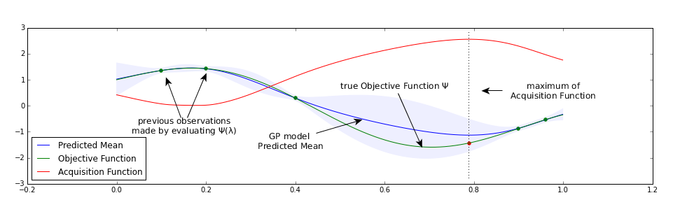
Since every evaluation of $\Psi$ with respect to a certain $\lambda$ incurs high cost, one goal should be to minimize their number. In Bayesian Optimization, a surrogate model is built to approximate the objective function $\Psi$ . Nearly all of the Bayesian Optimization literature uses Gaussian Processes as a surrogate function. This is constructed from already evaluated samples.
The next candidate hyperparameter values to be evaluated is obtained from the surrogate model using a utility or acquisition function $u$ .
Figure 1 illustrates these concepts. Following this procedure the problem of hyperparameter optimization now turns into the problem of maximizing the acquisition function $u$ .

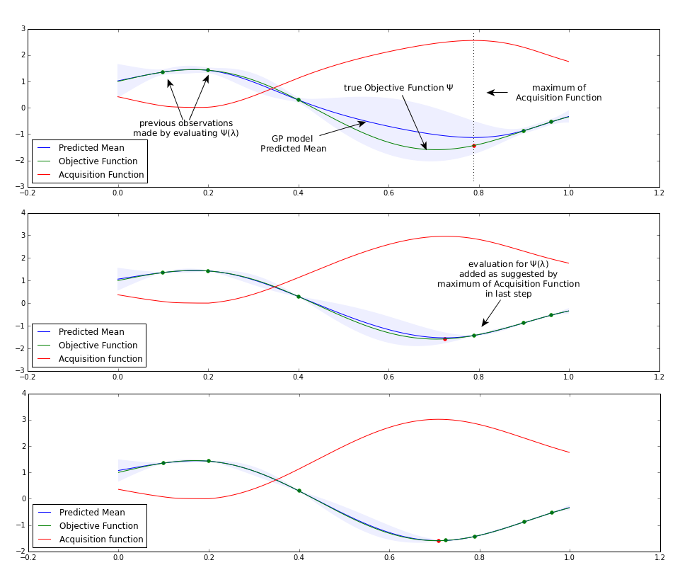
In total, the Bayesian Optimization procedure is shown in algorithm 1, and is also called sequential model based optimization algorithm (SMBO) in the literature.
In this algorithm, a model $M_{t}$ is used to approximate the complex response function $\Psi(\lambda)$ . The history of points where $\Psi$ has been evaluated is stored in $H$ . We run this algorithm for a fixed number of $T$ step. In each of the steps we first search the extremum of the acquisition function $u$ on the model $M_{t-1}$ . Afterwards, we execute the expensive evaluation of $\Psi$ at the found extremum $\lambda^{*}$ and add this evaluation to our history. Finally we use the updated history information to update $M_{t}$ . Figure 2 exemplarily shows this iterative approach for a one dimensional objective function.

1:function BayOpt(

\Psi

M_{0}

T

u

)

H\leftarrow\emptyset

;

3: for all

t\in\{1..T\}

\lambda^{*}\leftarrow argmin_{\lambda}\big{(}u(\lambda|M_{t-1})\big{)}

;

5: Evaluate

\Psi(\lambda^{*})

;

H\leftarrow H\cup\left(\lambda^{*},\Psi(\lambda^{*})\right)

;

M_{t}\leftarrow

refit surrogate model

M_{t-1}

to updated

H

;

8: end for

9: return

H

;

10:end function

Algorithm 1 Bayesian Optimization Algorithm [4]. Notation adapted.

2.1 Acquisition Functions

One of the most important design decisions is the acquisition function used to interpret the model. Most related papers introduce the Probability of Improvement function as a starting point and historical reference, but in general, Expected Improvement works significantly better in practice. Having implemented both of these functions, apsis uses Expected Improvement as a default.

2.1.1 Probability of Improvement

was first shown by Kushner [10] and states the simple idea of maximizing the probability to achieve any improvement by choosing $\lambda$ as a next point to sample from $\Psi$ .

\displaystyle u_{\text{PI}}(\lambda|M_{t})=\Phi\left(\frac{\mu_{M_{t}}(\lambda)-f(\lambda^{*})}{\sigma_{M_{t}}(\lambda;\theta)}\right)

(1)

That approach already indicates that it will favour exploitation of well-known areas over exploration of less-known regions of your optimization space $\Lambda$ .

2.1.2 Expected Improvement

A better criterion is the expected value of the actual improvement achieved when choosing to evaluate the objective for the next $\lambda$ value.

\displaystyle u_{\text{EI}}(\lambda|M_{t})=\underset{-\infty}{\int}^{\infty}\underbrace{max(y^{*}-y,0)}_{\text{value of improvement}}\text{ }\cdot\underbrace{p_{M}(y|\lambda)}_{\text{probability of improvement}}\text{ }dy

(2)

Since this integral cannot be directly computed, an analytical solution is helpful. For Gaussian Processes it has been shown [5, 16] that the analytical solution of basic EI is obtained as

\displaystyle u_{\text{EI}}(\lambda|M_{t})=\sigma(\lambda)\cdot\left(z(\lambda)\cdot\Phi(\lambda)+\phi(\lambda)\right)

(3)

using $z(\lambda)$ defined as

\displaystyle z(\lambda)=\frac{f(\lambda^{*})-\mu(\lambda)}{\sigma(\lambda)}

where $\mu(\lambda)$ and $\sigma(\lambda)$ are the mean and standard deviation as given from the Gaussian Process used. $\phi(\lambda)$ and $\Phi(\lambda)$ mark the standard normal distribution density and cumulative distribution function. Since apsis is supposed to handle both problems of maximization or minimization of the objective function both scenarios had to be incorporated into the acquisition function. Additionally, a trade-off parameter $\zeta$ to control the exploitation/exploration behaviour has been incorporated into $u$ as suggested in [5]. This leads to the following modified version of $z(\lambda)$ that is used in apsis, where $MAX$ is an integer being $1$ when the objective function has to be maximized and $0$ otherwise.

\displaystyle z(\lambda)=\frac{(-1)^{MAX}\cdot\left(f(\lambda^{*})-\mu(\lambda)+\zeta\right)}{\sigma(\lambda)}

2.2 Expected Improvement Optimization

One possibility for optimizing the acquisition function is to use gradient based optimization methods as they usually feature a better convergence speed than methods not relying on first order derivative information.

2.2.1 EI Gradient Derivation

Hence the gradient of EI had to be analytically derived. Applying the product rule to equation (3) one obtains

\displaystyle\nabla EI(\lambda)=

\displaystyle\text{ }\nabla\sigma(\lambda)\cdot\big{(}z(\lambda)\cdot\Phi(\lambda)+\phi(\lambda)\big{)}+\sigma(\lambda)\cdot\nabla\big{(}z(\lambda)\cdot\Phi(\lambda)+\phi(\lambda)\big{)}

(4)

\nabla EI(\lambda)=\frac{\nabla\sigma(\lambda)\cdot EI(\lambda)}{\sigma(\lambda)}\\ +\sigma(\lambda)\cdot\big{(}\nabla z(\lambda)\Phi(z)+\underbrace{z(\lambda)\phi(z)\cdot\nabla z(\lambda)-z(\lambda)\phi(z)\cdot\nabla z(\lambda)}_{=0}\big{)}

(5)

In the above $\nabla\phi(x)=-x\cdot\phi(x)$ has been used and the last two terms of the sum cancel out leading to the compact result

\displaystyle\nabla EI(\lambda)

\displaystyle=\frac{\nabla\sigma(\lambda)\cdot EI(\lambda)}{\sigma(\lambda)}+\sigma(\lambda)\cdot\big{(}\nabla z(\lambda)\Phi(z)\big{)}.

(6)

Finally, we compute the derivative of $z(\lambda)$ using the product rule.

	$\displaystyle\nabla z(\lambda)$	$\displaystyle=\frac{(-1)^{MAX}\cdot-\nabla\mu(\lambda)}{\sigma(\lambda)}-\frac{(-1)^{MAX}}{{\sigma}^{2}(\lambda)}\cdot\left(f(\lambda^{*})-\mu(\lambda)+\zeta\right)\cdot\nabla\sigma(\lambda)$		(7)
		$\displaystyle=\frac{(-1)^{MAX}\cdot-\nabla\mu(\lambda)}{\sigma(\lambda)}-\frac{z(\lambda)\cdot\nabla\sigma(\lambda)}{\sigma(\lambda)}$		(8)

It is more convenient for the implementation to have $\nabla\sigma^{2}(\lambda)$ instead of $\nabla\sigma(\lambda)$ , since the GP framework used in apsis returns both the mean and variance gradients. Fortunately, using the chain rule, one can derive

\displaystyle\nabla\sigma(\lambda)=\frac{\nabla\sigma^{2}(\lambda)}{2\sigma(\lambda)}

(9)

Using all of the above and inserting it in (6), the full EI gradient result is

\displaystyle\nabla EI(\lambda)

\displaystyle=\frac{\nabla\sigma^{2}(\lambda)}{2\sigma(\lambda)}-(-1)^{MAX}\cdot\nabla\mu(\lambda)\cdot\Phi(z(\lambda))-\nabla\sigma^{2}(\lambda)\cdot\Phi(z(\lambda))\cdot\frac{z(\lambda)}{2\sigma(\lambda)}

which is the formula implemented in apsis.

2.2.2 Available Optimization Methods

The following gradient and non-gradient based optimization methods are available in apsis.

•

Quasi-Newton optimization using inverse BFGS [20, p. 72]
•

Limited Memory BFGS with bounds algorithm (default) [6]
•

Nelder-Mead method [12]
•

Powell method [15]
•

Conjugate Gradient method [13]
•

inexact/truncated Newton method using Conjugate Gradient to approximately solve the Newton Equation [20, p. 62] [13]
•

random search

Except for random search the implementations of these methods are taken from the SciPy project [8]. In order to provide these methods with a promising starting point $\lambda_{0}$ a random search maximization is always executed first and the best resulting $\lambda$ will be used as $\lambda_{0}$ for any of the further optimization methods.

The BFGS method marks the strongest of these methods and offers the best convergence speed since it uses gradient information and approximates the second order information. Similar to the original Newton method it computes the next optimization step $s_{k}$ by solving the Newton equation

\displaystyle\nabla^{2}f(\lambda_{k})\cdot s_{k}=-\nabla f(\lambda_{k})

(10)

but as a so called Quasi Newton method it tries to approximate the Hessian $\nabla^{2}$ . Therefore it maintains the Quasi Newton equation (11) satisfied in every step to make sure $H$ provides a well enough approximation for the Hessian.

\displaystyle H_{k+1}\cdot(\lambda^{k+1}-\lambda^{k})=\nabla f(\lambda^{k+1})-\nabla f(\lambda^{k})

(11)

Since equation (10) can be solved for $s_{k}$ by inverting the Hessian, the inverse BFGS method used in apsis directly approximates the inverse of the Hessian using an iterative algorithm to speed up optimization.
It will however not always converge since the algorithm involves a division by something that can become $0$ [20, p. 72]. In that case the algorithm stops gracefully with an error and apsis relies on the random search result. Since the optimization space is bounded in real settings apsis by default uses an adopted version of BFGS, the L-BFGS-B [6] algorithm. In contrast to ordinary BFGS it does not store the full $n\times n$ Hessian but only stores a few vectors to implicitly represent the Hessian approximation $H$ . Furthermore it has been extended by Byrd et al. [6] to respect simple bounds constraints for each variable definition which is sufficient for the bounds used in apsis.

3 Architecture

3.1 General Architectural Overview

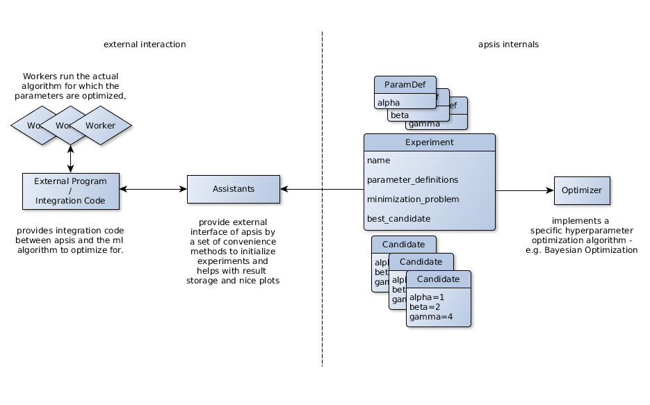
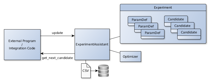
The architecture of apsis is designed to be interoperable with any Python machine learning framework or self-implemented algorithm. apsis features an abstraction layer for the underlying optimization framework as depicted in figure 3. Every optimizer adheres to the abstract base class Optimizer. The optimizer uses three important model classes to control optimization. Candidate is used to represent a specific hyperparameter vector $\lambda$ . Experiments are used to define a hyperparameter optimization experiment. An Experiment holds a list of ParamDef objects that define the nature of each specific hyperparameter. The external program interacts with apsis through a set of Assistants. They help to initialize apsis’ internal structure and models and provide convenient access to optimization results, and can optionally store and plot them or compare several experiments. Additionally, the external program has to provide some integration code between the external program’s machine learning algorithm and the apsis interface. Since the external program could be multi-threaded or clustered apsis refers to the processes running the machine learning algorithms as Workers.

On the implementation level apsis is made up by six packages reflecting this architecture. Table 1 lists all of them and briefly describes their purpose.

Package

Description

Contents

assistants

Contains lab and experiment assistants for

apsis’ external interface.

experiment_assistant.py

lab_assistant.py

optimizers

Contains all available optimizers and the abstract

base class. Contains a subpackage for

Bayesian Optimization.

optimizers.py

random_search.py

bayesian_optimization.py

bayesian/acquisition_functions.py

models

Contains the model classes.

candidate.py

experiment.py

parameter_definition.py

tests

Contains unit tests for complete apsis code.

test_assistants/…

test_models/…

test_optimizers/…

test_utilities/…

utilities

Utility functions used accross all packages.

benchmark_functions.py

file_utils.py

import_utils.py

logging_utils.py

optimizer_utils.py

plot_utils.py

randomization.py

demos

Some demos intended for learning how to

use apsis by examples.

demo_MNIST.py

demo_MNIST_MCMC_py

Table 1: list of apsis packages with their purpose and contents

3.2 Model Objects

3.2.1 Candidate

represents a specific hyperparameter vector $\lambda$ and optionally stores the result of the objective function $\Psi(\lambda)$ achieved under this $\lambda$ if already evaluated. Additionally it can store the cost occurred for evaluation and any other meta information used by the worker, e.g. the worker could keep track of the classifier’s weights in each step and store them there. The actual vector $\lambda$ is stored as a dictionary such that every parameter dimension $\lambda^{(i)}$ is named.

3.2.2 Experiment

stores information about the nature of the parameters to be optimized, defines if the problem is for minimization and maximization. It keeps track of successfully evaluated, currently evaluated and to be evaluated Candidates. It stores the best Candidate and optionally names the experiment.
Additionally, it provides methods for semantic check if candidates are valid for this experiment, and can convert itself to a CSV format for result storage.

3.2.3 ParamDef

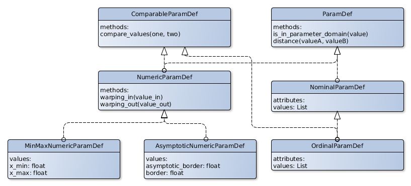
is the most general superclass used to define the nature of one hyperparameter dimension. It makes no assumption on the nature of the stored parameter. NominalParamDef defines non-comparable, unordered parameters and stores all available values in a list. OrdinalParamDef represents ordinal parameters where the order is maintained by the position in the list of values. As ordinal parameters can be compared they adhere to the ComparableParamDef interface and provide a compare_values function that provides similar semantic to the Python integrated __cmp__ function. Furthermore, apsis comes with special support for numeric parameters represented by the NumericParamDef class. Numeric param defs are comparable and are represented internally by a warping into the $[0,1]$ domain. Hence they need to be given an inwards and outwards warping function. The warped parameters are now compared and treated according to the rules of treating ordinary floats between $0$ and $1$ . To ease initialization of numeric parameters MinMaxNumericParamDef automatically provides a warping assuming an equal distribution of the parameter between the given minimal and maximal value. AsymptoticNumericParamDef provides a parameter definition for a parameter which is expected to be close to one value. For example, learning rates can be estimated as being close to 0. This leads to significantly better results during optimization, as long as some expert knowledge is available.
Figure 4 depicts the structure of available parameter types and there inheritance relationships.

3.3 Optimization Cores

The abstract base class Optimizer defines the common interface of any optimization algorithm provided in apsis. Central is the method get_next_candidates. Based upon information stored in the given experiment instance the method provides its user with one or several promising candidates to evaluate next. On construction the optimizer can receive a dictionary of optimizer specific parameters to define optimization related hyperparameters. Note that these parameters are not the ones that are subject of optimization but are parameters to govern the optimization behaviour such as which acquisition function or kernel is used in Bayesian Optimization. apsis provides two different optimization cores: a simple random search based optimizer called RandomSearch and the SimpleBayesianOptimizer.

3.3.1 RandomSearch

Implements a very simple random search optimizer. For parameters of type NumericParamDef a uniform random varibale between $0$ and $1$ is generated to select a value in warped space for each parameter. For parameters of type NominalParamDef a value is drawn uniformly at random from the list of allowed values. All random numbers are generated using the numpy [7] random package.

3.3.2 SimpleBayesianOptimizer

The SimpleBayesianOptimizer works according to the theory described in chapter 2. It is called simple since it currently works with one concurrent worker at a time only (though a multi worker variant is planned). It uses Gaussian Processes and their kernels provided by the GPy framework [1]. For the acquisition functions implemented and the methods in use for their optimization it shall be referred to chapter 2.1 and 2.2.

3.4 Experiment Assistants

The BasicExperimentAssistant provides the simplest interface between apsis and the outside world. It administers at most one experiment at a time. An experiment needs to be initialized by at least specifying a name to identify it, the Optimizer to be used and a list containing one ParamDef object for each hyperparameter to be optimized. It holds and manages the Optimizer and Experiment instances and provides an abstraction layer to their interface.

The experiment assistants provide the two methods get_next_candidate and update that should be called by the external program when it is ready to evaluate a new candidate or wants to notify apsis about work on a Candidate. The Candidate doesn’t necessarily need to be one which was provided by apsis but can be any Candidate which adheres to the parameter space. Furthermore BasicExperimentAssistant cares for storing the results to CSV files when running to be sure to have all information available after termination or abortion of an experiment run. The behaviour of the CSV writing can be controlled upon initialization of the experiment assistant. As an extension apsis provides PrettyExperimentAssistant that can additionally create nice plots on the experiment. Chapter 4 shows some of these plots.

3.5 Lab Assistants

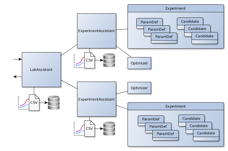
BasicLabAssistant deals with the requirement to run and control several experiments at once. It holds a dictionary of experiment assistants and provides a common interface to all of them following the same semantic as the experiment assistants themselves. The advantages of using lab assistants in contrast to controlling several experiments at the same time manually is that the results can now be stored together and compared. BasicLabAssistant provides only that function, while PrettyLabAssistant adds comparative plots for the comparison of multiple optimizers.

4 Evaluation

This section evaluates apsis on several benchmark and one real world example. All experiments are evaluated using cross validation and $10$ initial random samples that are shared between all optimizers in an experiment to ensure comparability.

4.1 Evaluation on Branin Hoo Benchmark Function

Some recent papers on Bayesian Optimization for machine learning publish evaluations on the Branin Hoo optimization function [16]. The Branin Hoo function

\displaystyle f_{\text{Branin}}(x)=a\cdot(y-b\cdot x^{2}+c\cdot x-r)^{2}+s\cdot(1-t)\cdot cos(x)+s

using values proposed in [18] is defined as

\displaystyle f_{\text{Branin}}(x)=(y-\frac{5.1}{4\pi^{2}}\cdot x^{2}+\frac{5}{\pi}\cdot x-6)^{2}+10\cdot(1-\frac{1}{8\pi})\cdot cos(x)+10.

In contrast to our expectations Bayesian Optimization was not able to outperform random search on Branin Hoo. Still the result is much more stable and the bayesian optimizer samples only close to the optimum.

4.2 Evaluation on Multidimensional Artificial Noise Function

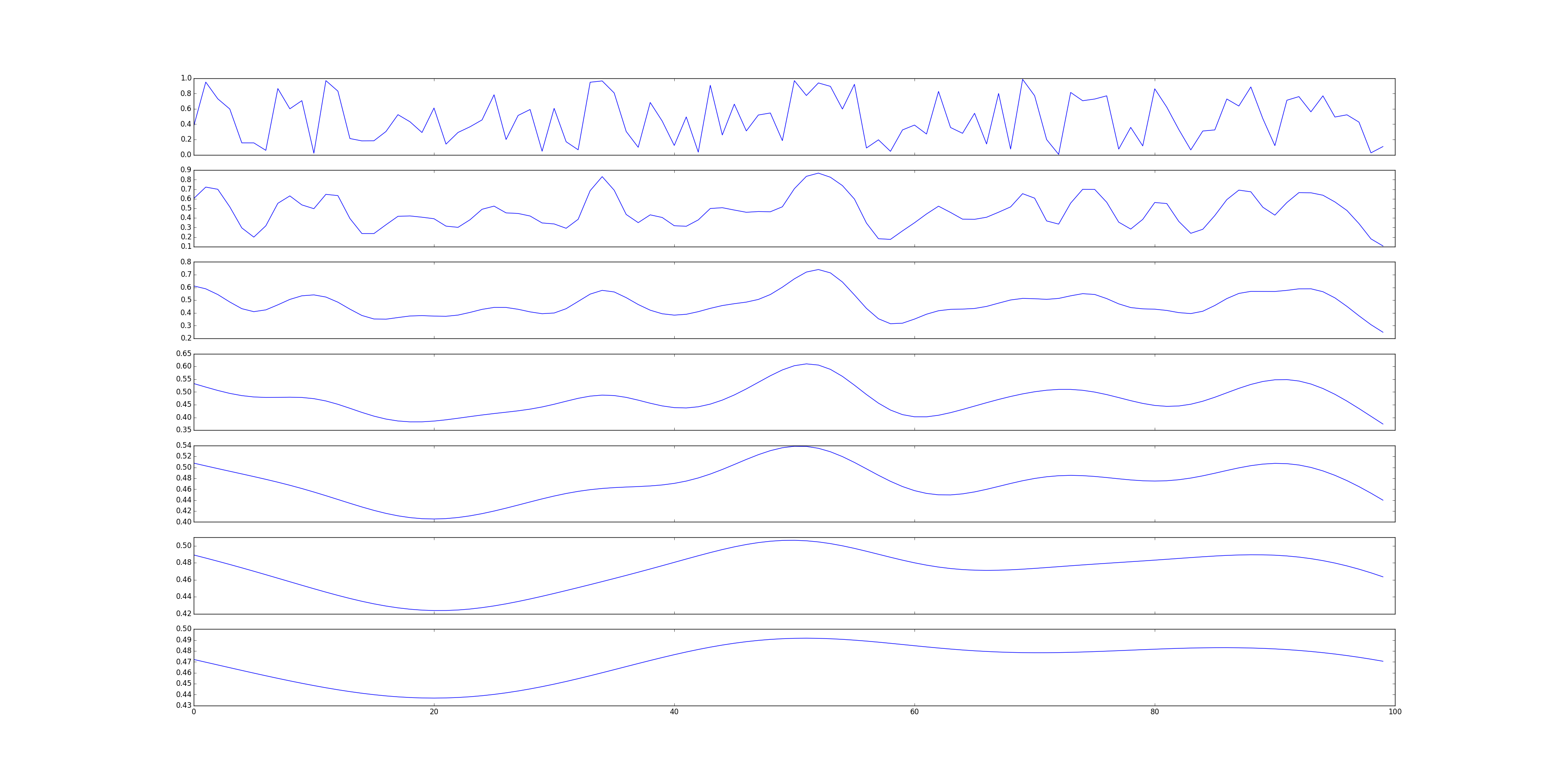
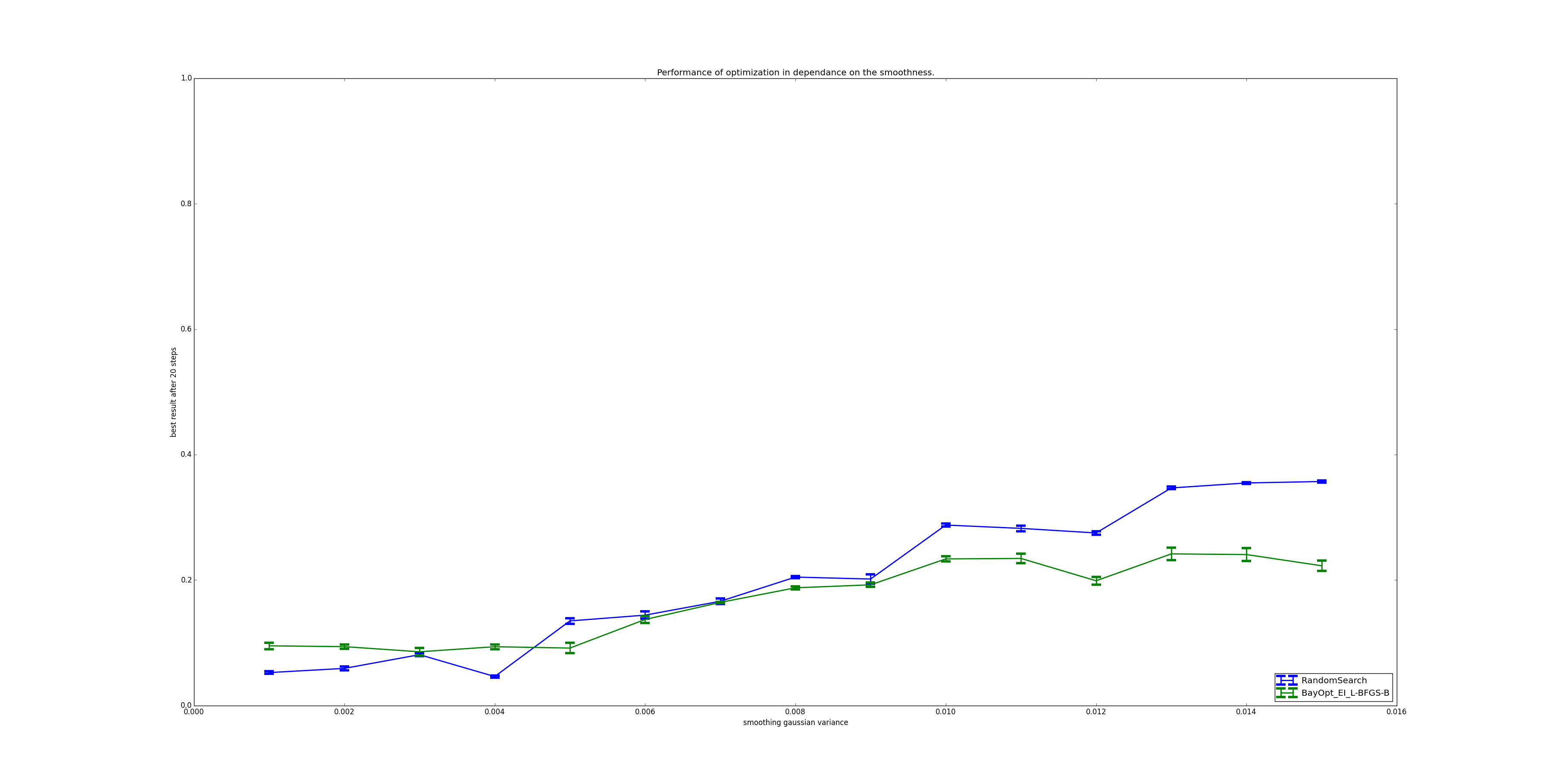
Compared to random search an intelligent optimizer should be better on less noisy function than on very noisy functions in theory. A very noisy function has a tremendous amount of local extrema making it hard to impossible for Bayesian Optimization methods to outperform random search. To investigate this proposition an artificial multidimensional noise function has been implemented in apsis as shown in figure 9.
Using this noise function, one can generate multi-dimensional noises with varying smoothness. The construction process first constructs an $n$ -dimensional grid of random points, which remains constant under varying smoothness. Evaluating a point is done by averaging the randomly generated points, weighted by a gaussian with zero mean and varying variance¹¹1Actually, only the closest few points are evaluated to increase performance.. This variance influences the final smoothness. A one-dimensional example of generated functions for differing variances is seen in figure 9.
The result can be seen in figure 9. As expected, Bayesian Optimization outperforms random search for smoother functions, while achieving a rough parity on rough functions.

4.3 Evaluation on Neural Network on MNIST

To evaluate the hyperparameter optimization on a real world problem, we used it to optimize a neural network on the MNIST dataset [11]. We used Breze[9] as a neural network library²²2Breze uses theano [3, 2] in the background. in Python.
The network is a simple feed-forward neural network with 784 input neurons, 800 hidden neurons and 10 output neurons. It uses sigmoid units in the hidden layers, and softmax as output. We learn over 100 epochs. These parameters stay fixed throughout the optimization.
For assigning the neural network weights, we use a backpropagation algorithm. Its parameters - step_rate, momentum and decay - are optimized over, as is $c_{wd}$ , a weight penalty term. Hence, resulting in a four dimensional hyperparameter optimization.
We ran all neural network experiments with a five-fold cross validation. Even so, total evaluation time ran close to 24 hours on an Nvidia Quadro K2100M.
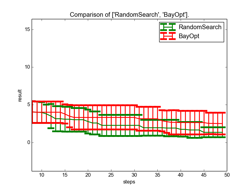
Figure 10 shows the performance of the optimizers for each step. As can be seen, Bayesian Optimization - after the first ten, shared steps, rapidly improves the performance of the neural network by a huge amount. This is significantly more stable than the random search optimizer it is compared with.

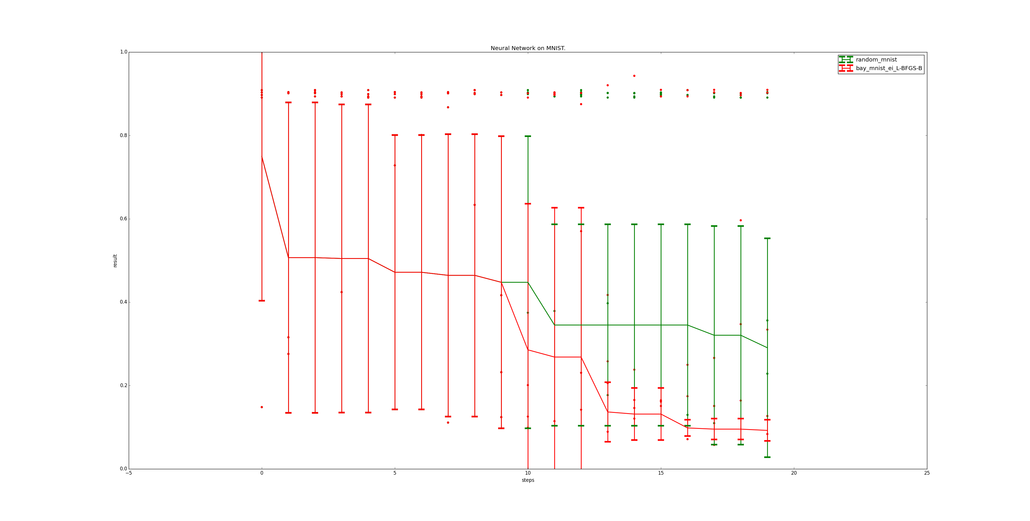
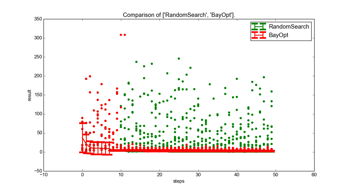
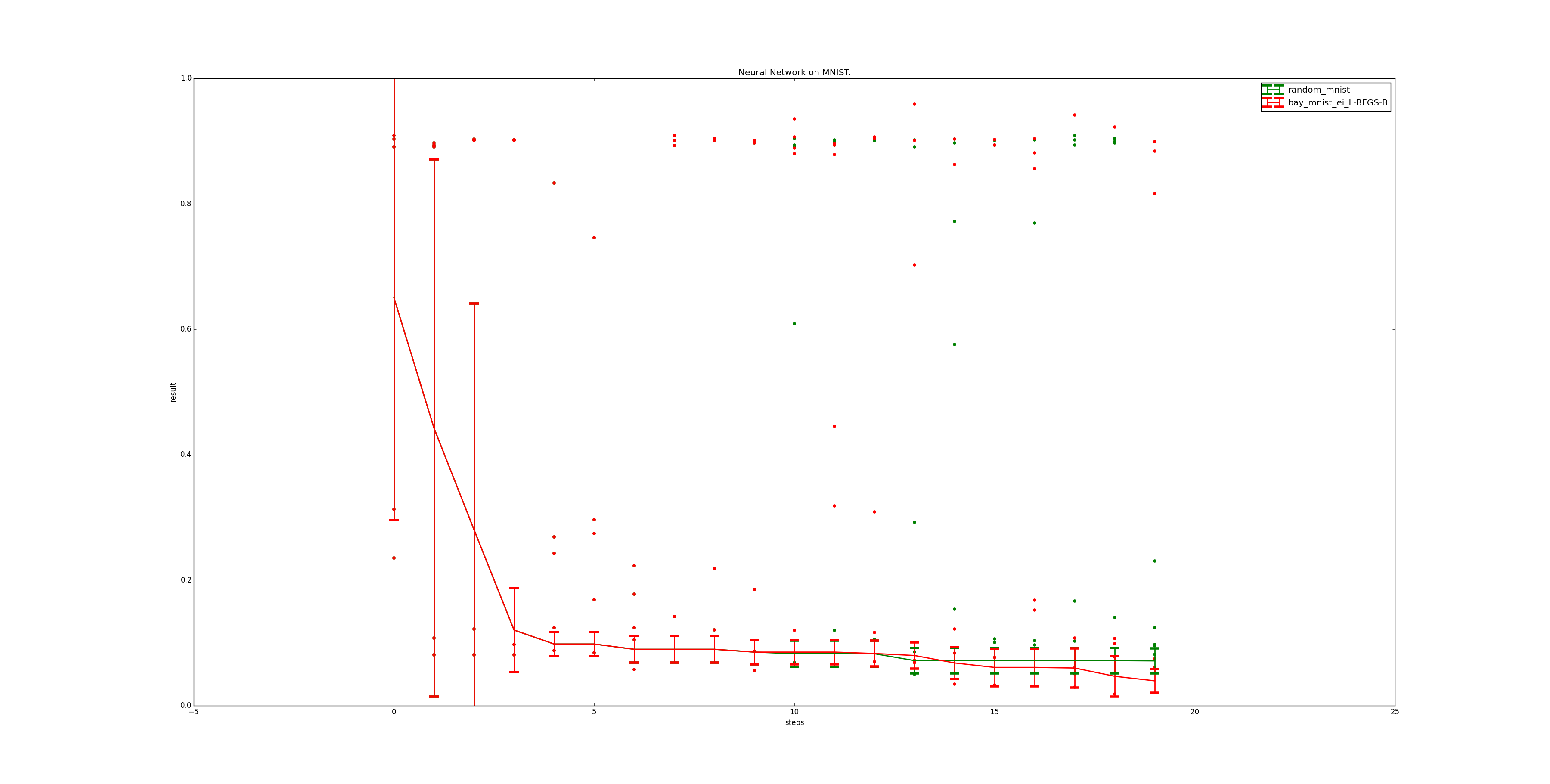
However, the optimization above uses no previous knowledge of the problem. In an attempt to investigate the influence of such previous knowledge, we then set the parameter definition for the step_rate to assume it to be close to 0, and the decay to be close to 1. This is assumed to be knowledge easily obtainable from any neural network tutorial.
The effects of this can be seen in figure 11, and are dramatic. First of all, even random search performs significantly better than before, reaching a similar value as the uninformed Bayesian Optimization. Bayesian optimization profits, too, and decreases the mean error by about half.

5 Conclusion

With apsis we presented a flexible open source framework for optimization of hyperparameters in machine learning algorithms. It implements most of the state of the art on hyperparameter optimization of current research and is open for further extension.
It is our hope that apsis will continue to be expanded, and will be used extensively in academia.

The performance evaluation justifies that Bayesian Optimization is significantly better than random search on a real world machine learning problem. Furthermore the need for an efficient parameter optimization arises already on an experiment with only fifteen minutes of computation time per evaluation. These settings will certainly be met by any practical machine learning problem. Including very simple prior knowledge of the algorithm leads to another significant performance improvement.

There are several areas in which apsis can be further improved. We would like to implement support for multiple concurrent workers, allowing us to optimize on clusters. Adding a REST web-interface allows an easy integration of apsis to arbitrary languages and environments.
There also remain possible improvements on the implemented bayesian optimizer itself. [19] propose using early validation to abort the evaluation of unpromising hyperparameters. [17] propose learning input warpings, which would further reduce the reliance on previous knowledge. [16] use a cost function to minimize total computing time instead of the number of evaluations. The problem generally known as a tree-structured configuration space as pointed out by [4] could be tackled, allowing us to mark parameters as unused for a certain evaluation. Student-t processes might be investigated as a replacement for gaussian processes. Lastly, adding efficient support for nominal parameters in Bayesian Optimization is important for a good performance, though since no publication on that topic exists so far this might be one of the biggest barriers to tackle.

References

authors [2012–2014] The GPy authors. GPy: A gaussian process framework in python. http://github.com/SheffieldML/GPy, 2012–2014.
Bastien et al. [2012] Frédéric Bastien, Pascal Lamblin, Razvan Pascanu, James Bergstra, Ian J. Goodfellow, Arnaud Bergeron, Nicolas Bouchard, and Yoshua Bengio. Theano: new features and speed improvements. Deep Learning and Unsupervised Feature Learning NIPS 2012 Workshop, 2012.
Bergstra et al. [2010] James Bergstra, Olivier Breuleux, Frédéric Bastien, Pascal Lamblin, Razvan Pascanu, Guillaume Desjardins, Joseph Turian, David Warde-Farley, and Yoshua Bengio. Theano: a CPU and GPU math expression compiler. In Proceedings of the Python for Scientific Computing Conference (SciPy), June 2010. Oral Presentation.
Bergstra et al. [2011] James Bergstra, Rémy Bardenet, Yoshua Bengio, and Balázs Kégl. Algorithms for hyper-parameter optimization. In NIPS’2011, 2011.
Brochu et al. [2010] Eric Brochu, Vlad M. Cora, and Nando de Freitas. A Tutorial on Bayesian Optimization of Expensive Cost Functions, with Application to Active User Modeling and Hierarchical Reinforcement Learning. IEEE Transactions on Reliability, abs/1012.2, 2010.
Byrd et al. [1995] Richard H. Byrd, Peihuang Lu, Jorge Nocedal, and Ciyou Zhu. A limited memory algorithm for bound constrained optimization. SIAM J. Sci. Comput., 16(5):1190–1208, September 1995. ISSN 1064-8275. doi: 10.1137/0916069. URL http://dx.doi.org/10.1137/0916069.
Dubois et al. [1996] Paul F. Dubois, Konrad Hinsen, and James Hugunin. Numerical python. Computers in Physics, 10(3), May/June 1996.
Jones et al. [2001–] Eric Jones, Travis Oliphant, Pearu Peterson, et al. SciPy: Open source scientific tools for Python, 2001–. URL http://www.scipy.org/. [Online; accessed 2015-02-23].
Justin Bayer [2015] Sebastian Urban Moritz August Adrià Puigdomènech Badia Justin Bayer, Christian Osendorfer. Breze: A gradient based learning framework in python. https://github.com/breze-no-salt/breze, 2015.
Kushner [1964] Harold J Kushner. A new method of locating the maximum point of an arbitrary multipeak curve in the presence of noise. Journal of Fluids Engineering, 86(1):97–106, 1964.
[11] Yann Lecun and Corinna Cortes. The MNIST database of handwritten digits. URL http://yann.lecun.com/exdb/mnist/.
Nelder and Mead [1965] J. A. Nelder and R. Mead. A simplex method for function minimization. The Computer Journal, 7(4):308–313, January 1965. ISSN 1460-2067. doi: 10.1093/comjnl/7.4.308. URL http://dx.doi.org/10.1093/comjnl/7.4.308.
Nocedal and Wright [1999] J. Nocedal and S.J. Wright. Numerical Optimization. Springer series in operations research and financial engineering. Springer, 1999. ISBN 9780387987934. URL http://books.google.de/books?id=epc5fX0lqRIC.
Pedregosa et al. [2011] F. Pedregosa, G. Varoquaux, A. Gramfort, V. Michel, B. Thirion, O. Grisel, M. Blondel, P. Prettenhofer, R. Weiss, V. Dubourg, J. Vanderplas, A. Passos, D. Cournapeau, M. Brucher, M. Perrot, and E. Duchesnay. Scikit-learn: Machine learning in Python. Journal of Machine Learning Research, 12:2825–2830, 2011.
Powell [1964] M. J. D. Powell. An efficient method for finding the minimum of a function of several variables without calculating derivatives. The Computer Journal, 7(2):155–162, January 1964. doi: 10.1093/comjnl/7.2.155. URL http://dx.doi.org/10.1093/comjnl/7.2.155.
Snoek et al. [2012] Jasper Snoek, Hugo Larochelle, and Ryan P Adams. Practical bayesian optimization of machine learning algorithms. In NIPS, pages 2960–2968, 2012.
Snoek et al. [2014] Jasper Snoek, Kevin Swersky, Richard S Zemel, and Ryan P Adams. Input warping for bayesian optimization of non-stationary functions. arXiv preprint arXiv:1402.0929, 2014.
[18] S. Surjanovic and D. Bingham. Virtual library of simulation experiments: Test functions and datasets. Retrieved March 9, 2015, from http://www.sfu.ca/~ssurjano.
Swersky et al. [2014] Kevin Swersky, Jasper Snoek, and Ryan Prescott Adams. Freeze-thaw bayesian optimization. arXiv preprint arXiv:1406.3896, 2014.
Ulbrich and Ulbrich [2012] M. Ulbrich and S. Ulbrich. Nichtlineare Optimierung. Mathematik Kompakt. Springer Basel, 2012. ISBN 9783034601429. URL http://books.google.de/books?id=pmfFbwAACAAJ.