[new=char=Q,reset char=R]counters
Architecture, Dataflow and Physical Design Implications of 3D-ICs for DNN-Accelerators
Abstract
The everlasting demand for higher computing power for deep neural networks (DNNs) drives the development of parallel computing architectures. 3D integration, in which chips are integrated and connected vertically, can further increase performance because it introduces another level of spatial parallelism. Therefore, we analyze dataflows, performance, area, power and temperature of such 3D-DNN-accelerators. Monolithic and TSV-based stacked 3D-ICs are compared against 2D-ICs. We identify workload properties and architectural parameters for efficient 3D-ICs and achieve up to 9.14x speedup of 3D vs. 2D. We discuss area-performance trade-offs. We demonstrate applicability as the 3D-IC draws similar power as 2D-ICs and is not thermal limited.
I Introduction
Deep neural network (DNN) inference demands high computation and is inherently parallel. Recently, the popularity of DNNs has given rise to specialized accelerators [1, 2]. Almost all DNN accelerators are matrix multiplication machines, since computation of DNNs follows this linear algebra motif, e.g., convolutions in CNNs (Convolution Neural Networks) or LSTM/GRU layers (Long Short Term Memory / Gated Recurrent Units) in Recurrent Neural Networks (RNNs).
The planar nature of modern accelerators allows two-dimensional parallelism. Executing operations with higher dimensions–e.g., convolutions with a batch size of one is a six-dimensional operation–requires unrolling the operands in 2D matrices, mapped along the two spatial dimensions and in time. This two-dimensional mapping limits the parallelism; Even with an infinitely large array, some operations must be executed sequentially.
We extend the accelerator to the third spatial dimension to increase its parallelism since the runtime can be reduced by remapping. Fig. 1 depicts the resulting 3D-accelerator, comprising layers of 2D systolic arrays stacked in 3D. The connections between the Multiply Accumulate Units (MACs) across the third dimensions (’tiers’) enable the entire 3D structure to work as a single unit. If there are no connections between the tiers, or these connections are not used during computation, then the accelerator works as a scaled-out 2D system, implemented using 3D technology.
Here, we study the impact of 3D-DNN accelerator in terms of computational and thermal performance, power, scalability, and area. We choose a logic-stacked systolic-array architecture for the sake of simplicity. We deliberately choose compute mappings that require communication across tiers so that the architecture is not equivalent to a scaled-out 2D system.
3D-Integrated Circuits (ICs) are fabricated either as a stacked 3D-IC, vertically interconnecting with Through-silicon-vias (TSVs), or a monolithic 3D-IC, vertically interconnecting with monolithic intertier vias (MIVs). Employing 3D-technology is challenging because of reduced yield vs. 2D, large area requirements of TSVs, and severe thermal limitations [3]. There are worthy benefits, e.g., less power consumption vs. 2D [4]; Even fundamental limits of computation are tackled [5]. Therefore, 3D integration is being introduced by industry at time of writing this paper: For example, Intel “Lakefield”, in which Foveros 3D technology is used to stack multicore processors and DRAM [6]. However, there is still a lack of research on the advantages of 3D integration on DNN-accelerators.
To investigate 3D integration for DNN accelerators, we created a 3D-systolic array analytical model. Our results shows that a 3D-accelerator gets a 9.14 speedup compared with a 2D one with same number of compute units. We also design a 3D systolic array in RTL and perform post-synthesis area, power, and thermal analyses. We show that performance benefits for 3D are nullified by area costs in some configurations. The power analysis depicts that the array consumes similar amount of power as in 2D; while the thermal performance of 3D is worse than 2D, it is still feasible.
In this paper we claim the following contributions:
-
•
We extend an analytical performance model from 2D to 3D that allows to optimize parameters such as tier count, computational resources and array dimensions for a given workload.
-
•
We conduct a power, performance, and area (PPA) analysis from an RTL implementation for real workloads comparing 2D against 3D with TSVs and 3D with MIV.
-
•
We use the RTL model to conduct a thermal study. 2D is compared vs. 3D (TSV and MIV).
II Related Work
Kung et al. [7] propose a 3D systolic array by folding a 2D one. Dataflows are essentially equivalent to 2D within each tier. This results in performance advantages from: A scale-out approach, reduced link lengths comparing TSVs to wires and concatenating the execution of NN layers. Unlike this work, [7] does not utilize 3D to leverage spacial parallelism in the temporal domain. MIVs are not analyzed.
Wang et al. [8] propose a systolic cube. The 3D topology is identical this work. The key differences are: the cube is implemented on a 2D IC and therefore is limited in scalability from wire length; the proposed dataflow targets 3D convolution. Our approach is more general such that any matrix multiplication is paralellized exploiting the extra spatial dimension enabled by the 3D substrate. The dataflow of [8] can be used in our 3D-IC, as well. Rahman et al. [9] propose a logical 3D array implemented on a 2D-IC. MACs within a layer (loosely analog to tiers) are not connected as each MAC maps one neuron.
TETRIS [10] implements a NN accelerator in the logic layer of 3D stacked memory. The array is a 2D topology. The approach saves memory traffic and reduces power.
Lakhani et al. [11] parallelize matrix multiplication in 3D. Although conceptually similar, [11] does not target the specific requirements of NN. Furthermore, the parallelization scheme along the third dimension relays on splitting up operations for floating point arithmetic among tiers, but each tier gets the whole set of inputs. Their proposed performance model is limited to matrices as big as the systolic array. The 3D array is not implemented; reliable area, power and thermal figures are not presented. Furthermore, a comparison of TSV and MIV-based implementations is not given.
III 3D Systolic Array for NNs
III-A Architecture
The architecture of our 3D systolic array is shown in Fig. 1. The MACs are connected to direct neighbors; horizontally via wires and vertically via TSVs/MIVs. The whole array calculates a matrix multiplication. Matrices can enter from top and left, shown in purple and orange. The matrix multiplication is parallelized in the third dimension by splitting it into partial sums. Thus, each layer is entered by two corresponding parts of the input matrices. The MAC units in the layer generate a partial sum. At the end, each pile of stacked MACs accumulates the data; then, the bottom layer returns the output matrix. (Other schemes would not require vertical communication, and our system was equivalent to a scaled-out accelerator.) This is shown in blue in Fig. 1 for one exemplary MAC pile. Only minor modifications to the MAC unit in comparison to a 2D array are necessary: One MUX, the accumulate control signal (partial summing across layers) and the vertical links are added.
Please note that we connect each pair of adjacent MACs with a TSV/MIV array between layers. In general, this is a over-provision of vertical interconnects that induces an area overhead (especially for TSVs) and reduces the chip’s yield. However, we chose this deliberately, as it is a worst-case approximation for 3D DNN-accelerators. Many methods that reduce the area overhead and increase the yield by limiting the number of vertical links exist in the literature (e.g., [12]). We do not discuss these here, as it is outside of the scope of this paper and existing approaches can be applied.
III-B Memory
The 3D accelerator talks to the external memory using a memory controller connected in one of the array’s layers. The requested data coming from outside of the chip is distributed to the layers in a fashion similar to one in [7], in which the small systolic arrays are distributed in 3D among dies [7, Fig. 7]. The 3D array profits of a one to two orders of magnitude smaller wire delay for these vertical interconnects [7, Fig. 8].
Data are stored intermediately before being fed into the array in scratchpad memory (cf. [13, Fig. 1]). There are two options: Either, there is SRAM on one tier that interconnects to all tiers; or each tier has dedicated SRAM. Both are possible due to the small wire delay for 3D [7]. As the size and architecture of the scratchpad memory has a vast influence on the performance, this has already been optimized for 2D, e.g., [13]. Those findings can also be applied here. Hence, the architecture and the parameters of scratchpad memory are outside of the scope of this paper.
To summarize, we do not claim any contribution in the memory system for a 3D systolic array and refer to the existing architectures proposed in the recent literature. For main memory, [7] proved a performance advantage of 3D-ICs. For scratchpad memory, the findings of 2D-ICs can be applied, as each tier has dedicated memory.
III-C Mapping/Dataflow
The mapping of operands plays an important role in determining the performance of a workloads on an accelerator. Chen et al. [1] describe the various mapping strategies in DNN accelerators and introduce a naming convention used here. [13] shows that out of the various strategies, three ones lend themselves for efficient mapping of computation on systolic arrays. These are output stationary (OS), weight stationary (WS) and input stationary (IS). In the following paragraphs we briefly describe these in the context of mapping a General Matrix Matrix Multiplication (GEMM) of two operand matrices and , and discuss the implications when mapped onto a 3D systolic architecture.
WS and IS dataflows. In the WS dataflow the elements of the matrix are first stored to the local memory of the MAC units, such that each column of the array gets the element corresponding the a specific col of the matrix B (given sufficient MACs). Once the elements are stored, one element of a row of the transposed matrix of is fed in from the left side of the array in each cycle. Each MAC then multiplies the incoming element with its stored operand, and forwards incoming value to the MAC unit on its right. The generated product is then added with the incoming sum from the top edge, and the partial sum is sent to the element on the bottom row. Thus, the elements corresponding to each column of the output are generated, within one column of the array, by reducing across the rows. To summarize this strategy, the dimension is mapped spatially along the columns, the dimension is also mapped spatially along the rows. However, the dimension is temporally mapped.
The IS dataflow is similar to WS, but the mapping of matrices and are interchanged. The elements of each row in matrix are first stored into the local memory of MACs along array columns. The columns of matrix are then fed in from the left, one column per cycle, and the multiplication and reduction takes place similar to the case in WS. Thus, the dimension is mapped spatially along the array columns. The dimension is also mapped spatially along the array rows, while the dimension is mapped temporally.
OS dataflow. The elements of matrix are streamed from the top edge of the array, such the each column of this matrix send to a particular array column; while the elements of matrix are streamed from the left edge of the array such that each array row receives elements from the corresponding row of the operand. The partial sums are generated in each MAC and are reduced locally, producing the output matrix. Fig. 4 depicts the schematics of this mapping. To summarize, the dimensions and are mapped along the array’s spatial dimensions. The dimension is mapped along the temporal dimension.
Exploiting the third dimension. The analysis above shows that the temporal dimension contributes to increase in runtime and therefore impedes performance (given an optimal 2D mapping). Adding a third spatial dimension can alleviate this bottleneck. In the context of WS and IS dataflow, this translates to mapping the and dimension in the ‘new’ spatial dimension. E.g., if we have a 3D stacked architecture, of 2 planar arrays; in WS dataflow, half of the rows in matrix would be used in the ‘top’ tier array, while the other half in the ‘bottom’ tier array. In case of IS dataflow, the mapping would be similar, but the roles of matrix and would be interchanged. Please note that there is no communication between the arrays on the different tiers. This is identical to a distributed array, and such acceleration lends itself into the well studied model parallelism approach [13].
The OS dataflow, however, is an interesting one for 3D. Tthe dimension will be mapped to the third spatial dimension, therefore leading to reductions to be performed across the tiers. Fig. 4 depicts the computation flow equivalent to a single MAC on a 2D array, working with OS strategy on the proposed 3D setting. We refer to this new strategy as “distributed output stationary (dOS)". In Fig. 4 we show a schematic of a 2-tiered 3D array employing dOS dataflow. The mapping and reduction across various tiers lead to interesting architectural trade-offs to improve performance. The combination of inplace and cross-tier reduction means that naïvely increasing the number of tiers will lead to increased reduction time and will hamper performance (see Sec. IV-A). In the rest of this paper, we focus on the dOS dataflow and study the performance and implementation aspects in a 3D systolic array setting. We do not dive into details for the WS and IS dataflows as the existing literature on model parallelism provides detailed analysis for these cases [1].
III-D Analytical performance model
In [13], an analytical performance model has been proposed: For a 2D systolic array with rows and columns (i.e. MACs) and workload matrices of dimensions , and , [13, Eq. (4)] gives the calculation time:
| (1) |
Given large matrix sizes such that the given 2D array could not map the entire computation at once, serialization is required. The dimension will be mapped across the rows, if in case the number of rows is insufficient. The entire mapping requires steps. Similarly dimension is mapped across the columns, leading to steps to complete the mapping. The total number of serial steps required is given by .
In each step of the serialization it takes () cycles to fill the entire array, since the elements of IFMAP and Filter matrices are fed simultaneously. In OS dataflow the computation for each OFMAP pixel is done in-place within a MAC unit, thus it requires cycles to generate one OFMAP pixel. Since multiple MAC units are running in parallel, the latency of computation can be hidden for all but one MAC unit, which gets the data at the end. This MAC takes another cycles after the array is filled. Once all the computation is finished, it takes another cycles to remove all the generated outputs from the array. The term, () therefore indicates the runtime for a single serial step or fold. The authors also propose an optimization method to find the optimal array sizes for a given workload that minimizes this runtime.
The given formula naturally extends to a third dimension. Using the OS dataflow for 3D, the work among tiers is split up in -dimension, i.e. along in the workload. The workload is not split up along and . Thus, each of the tiers works on the partial sums with an input workload matrix dimension of , and . At the end, the partial sums are accumulated; this requires additions. This yields the following formula for the runtime of a 3D systolic array with rows per tier and columns per tier:
| (2) |
Please note that the constraint for the MAC count changed as the 3D array has MACs. Thus, the method from [13] can be applied to optimize the array dimensions for all tiers for the workload by changing the objective function to Eq. 2 and using MACs and a workload size of , and . To generate the distributed OS dataflow, each tier has the same array dimensions.
IV Results and Design Implications
We synthesized our RTL implementation for 15 nm nangate node (FreePDK15) [14] using Synopsys® Design Compiler; power analysis was done with post-synthesis with Synopsys® PrimeTime PX. The thermal analysis was done with HotSpot 6.0 [15]. For performance analysis, we sweep workload parameters and take the range of , and from typical DNNs. Exemplary workload parameters are shown in Table I.
| Name | Layer | |||
|---|---|---|---|---|
| Resnet50 [16] | RN0 | 64 | 12100 | 147 |
| RN1 | 512 | 784 | 128 | |
| Google’s neural mashine translation [17] | GNMT0 | 128 | 4096 | 2048 |
| GNMT1 | 320 | 4096 | 3072 | |
| DeepBench [18] | DB0 | 1024 | 50000 | 16 |
| DB1 | 35 | 2560 | 4096 | |
| Transformer [19] | TF0 | 31999 | 84 | 1024 |
| TF1 | 84 | 4096 | 1024 |
IV-A Performance
We compare the performance of 3D and 2D using Eq. 1 and Eq. 2. We assume an identical number of MACs that are evenly split up among tiers. (Eq. 1 holds with and Eq. 2 holds with .) We round down to avoid resource over-provision.
IV-A1 Workload parameters
The influence of , the inner dimension of the matrix-matrix product, is shown in Fig. 6. It depicts the speedup of a 3D-accelerator normalized to its 2D-counterpart with same MAC count (y-axis) depending on the tier count (x-axis). There are different curves for varying number of MACs (same color) and varying parameter (same shape). For each curve, and are fixed. The workloads are taken from a language recognition network (Resnet50).
The performance of the 3D array improves for larger and a fixed MAC count. 3D is not advantageous for a small and a small MAC count (e.g., and MACs), as of worse performance than in 2D (green plots). If is large, the 3D array yields a significant speedup. In best case, we see a speedup of up to 1.93 for 2 tiers and up to 9.16 for 12 tiers vs. 2D.
The influence of /, the outer dimensions of the matrix product are shown in Fig. 6. It depicts speedup of a 3D-accelerator normalized to its 2D-counterpart with same MAC count (y-axis) depending on a given budget of MACs, i.e., processing power (x-axis). We set the number of tiers to 4. There are different curves for varying (same color) and varying (same shape). The influence of and is symmetrical, so we only vary , while is constant.
The parameter and determine a threshold for a minimal MAC count required to gain a performance benefit from 3D; the threshold is marked with a dashed line. The threshold is given by (This was evaluated for reasonable tier counts 16, although not shown). We achieve a maximum speedup of 3.13 for the given parameter sets.
To summarize, the workload analysis shows that 3D arrays provide a large performance benefit vs. 2D for workloads with large and relatively small and . This is often the case, e.g., in language recognition models. The minimal MAC count to gain a speedup is given by .
IV-A2 Architectural parameters
The MACs count must be high to unleash 3D-integration, as shown In Fig. 6. For instance, for the workload with yields a 51% performance loss for MACs but up to 9.16 speedup for MACs compared against 2D.
Fig. 6 shows the required MAC budget for which 3D provides speedup as a dotted vertical line. For MAC budgets larger than the threshold, there is a continuous performance improvement until saturation, for which provision of additional computational power does not make sense.
Fig. 6 shows the influence of the tier count. More tiers continue the trend for a given workload, i.e., if the workload yields better 3D performance, more tiers further will improve the performance and vice versa. Local minima for different tier counts are artifacts of quantization.
Any speedup of 3D is reduced for very large tier counts as the reduction of partial sums overtakes the time of partial sum generation, cf. Eq. 2. As the tier count is limited by production, we do not further discuss this.
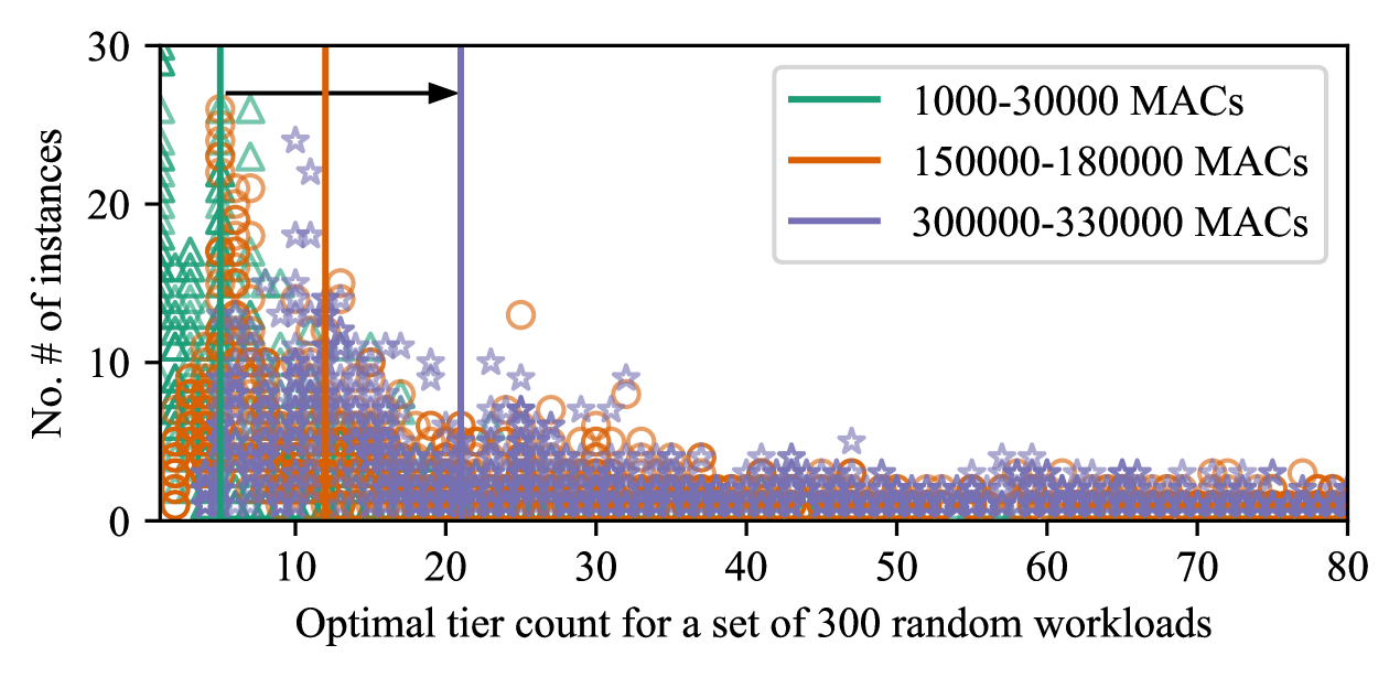
Fig. 7 show the combined influence of the tier count and MAC count. It is a scatter plot of the optimal tier count for a set of 300 random workloads based on Resnet50 parameters. The data are plotted for three MAC budgets resulting in a tail-heavy and shifted right distribution of the optimal tier count for larger MAC budgets. A vertical line shows the median of each distribution; the shift is highlighted by the black arrow. We conclude a trend that 3D arrays with larger MAC counts profit from larger tier counts.
To summarize, our architectural analysis shows that 3D is a viable choice for large system. Small devices with less than 4096 MACs will require other innovations to gain performance from 3D. 3D currently only targets high-performance systems such as servers due to high production costs so that our finding does not impede the practical application of 3D for DNN-accelerators. A high tier count would be favorable, although this is not realizable with current 3D manufacturing.
IV-B Power
We compare the power of a 3D-IC with TSVs or MIVs against a 2D-IC. TSVs have a very high capacitance of about 10fF [20], while MIV only have about 0.2fF capacitance [21].
We found that a static power analysis is insufficient. The reason lies in the special dataflow of a 3D-array, in which the horizontal links are heavily utilized while the vertical links are only used for partial sum accumulation. Hence, the switching activities of horizontal and vertical links vary.
We conduct post-synthesis power analysis for a 3-layer IC in 15 nm node with an example workload of = and = using Synopsys® PrimeTime PX.
The power consumption of an array with 16384 MACs per layer is shown in Tab. II (excluding power from data transmission from memory), along with the difference in power consumption vs. a 2D-IC with a similar total number of MACs (49284 MACs). We find that TSV-based 3D-IC requires 5.39% less power than a 2D-IC and a MIV-based 3D-IC requires 2.21% less power. As expected, MIVs are more frugal than TSVs.
3D-ICs do draw less power than 2D-ICs because of the special properties of the dataflow. This demonstrates the relevance of dynamic power analysis for 3D systolic arrays.
| Total Power | Peak Power | |||
|---|---|---|---|---|
| 2D | 6.61 W | — | 14.99 W | — |
| 3D TSV | 6.39 W | -5.4% | 14.41 W | -5.9% |
| 3D MIV | 6.26 W | -2.2% | 14.14 W | -2.1% |
IV-C Thermal Performance
As thermal performance is one of the most urgent issues of 3D integration [3], we conduct a thermal analysis with HotSpot 6.0 [15]. We chose a three-layer 3D-IC with 4096, 16384 and 65536 MACs per layer and a workload of and . The respective 2D-IC has as 12321, 49284 and 197136 MACs, which is approximately the MAC count of the 3D case.
The results are shown in Fig. 9 as a boxplot. For 3D, we split the data into the layer near the heatsink (bottom) and the rest (middle). The temperature variability comes from different switching activities and cooler MACs at the borders of the IC as of their fewer neighbors.
3D and 2D ICs get hotter for larger MAC counts. Furthermore, 3D ICs get hotter than 2D ICs. The TSV-based and the MIV-based 3D-ICs are not exceeding their thermal budget. This is a promising finding for 3D-ICs practically used for DNN-accelerators.
The MIV-based IC is hotter than the TSV-based IC. This is counter-intuitive due to the difference in parasitics of TSVs and MIVs. The reason lies in the vast number of vertical links. The large TSVs increase area, enhance heat dissipation and reduces the temperature. In a real system, one would apply TSV-saving schemes to improve area and yield, which will increase the temperature above the level of MIV-based ICs.
IV-D Area
We implement the 2D and 3D arrays in a 15 nm node with 8b inputs and 16b outputs for 1 GHz clock frequency. We take TSV area plus keep-out-zone (KOZ) from [20] and MIV area from [22].
The TSV-based 3D-IC is larger than the 2D array from additional area for logic, TSVs and KOZs. Monolithic integration only adds a few percent overhead vs. 2D, as no KOZs are required.
We plot the runtime per chip area to evaluate the area-impled trade-offs. This is plotted in Fig. 9 normalized against 2D for different tier counts for one exemplary given workload from Resnet50. Based on our previous discussion for runtime, we chose a workload that yields a performance benefit for 3D (=, =, =). The results are shown in Fig. 9 for a TSV-based (orange) and for a MIV-based (purple) 3D-IC.
For 4096 and 32768 MACs, the performance per area of the 3D-IC is worse by up to 75% than the 2D-IC. For 266144 MACs, the area per performance is improved for more than 4 layers by 1.27 to 2.83 (cf. 9). This finding underlines again that 3D integration is useful for large MAC counts.
We took a worst-case approach to the TSV count, as we provide a dedicated TSV array connecting each pair of MACs. If we apply TSV-reduction architectures (cf. Sec. III-A), TSV-based 3D-ICs will come off better.
MIV-based 3D-IC enable a better performance per area than TSVs: While the performance per area for 4096 MACs is similar to 2D-ICs, MIV-3D-ICs improve performance per area by up to 7.9 for larger MAC counts. The general trend is that higher MAC counts and number of tiers improve the performance advantage of 3D vs. 2D.
Two tiers with face-to-face bonding can be manufactured at time of writing this paper. For this, 3D integration allows for 1.19 to 1.97 better performance per area.
V Conclusion
In this paper, the implications of 3D-ICs for DNN-accelerators on their architecture, dataflow and design are analyzed. 3D-integration allows to add an additional level of spatial parallelism that is otherwise executed in the time domain for a 2D system. We choose a systolic-array based architecture and propose a 3D-implementation. We describe a suitable dataflow distributed output stationary that fully utilizes the capability of 3D and is not equivalent to existing data mappings for 2D. Using an analytical performance model and an RTL implementation for the 3D-array, we conduct an in-depth analysis about design implications in computational and thermal performance, area and power. Our analysis depicts that 3D-implementation enables performance improvements for DNN workloads. We identify a threshold for required computational performance to fully gain a speedup for 3D. The speedup is almost an order of magnitude (up to 9.14x) vs. 2D. From an architectural perspective, we find that a higher MAC count and more tiers improve the performance of 3D, while over-provisioning of computational resources leads to a speedup saturation vs. 2D. We show that thermal performance allows for 3D integration of DNN accelerators both with TSVs and MIVs. The area of a 3D accelerator is larger than 2D; but even for TSVs the performance per area is superior to 2D as MACs and tiers are scaled. Monolithic 3D integration naturally offers advantages over TSV-based stacking for area and power. To summarize, we conduct a comprehensive study on 3D-accelerators that is universal in that it abstracts from design details that are not purely related to vertical integration of DNN-accelerators such as memory and TSV-count.
References
- [1] Y.-H. Chen et al., “Eyeriss: An energy-efficient reconfigurable accelerator for deep convolutional neural networks,” in ISSCC, 2016.
- [2] N. Jouppi et al., “In-datacenter performance analysis of a tensor processing unit,” CoRR, vol. abs/1704.04760, 2017.
- [3] T. S. Perry, “Forget moore’s law—chipmakers are more worried about heat and power issues,” in IEEE Spectrum, 2019.
- [4] X. Dong and Y. Xie, “System-level cost analysis and design exploration for three-dimensional integrated circuits (3D ICs),” ASPDAC, 2009.
- [5] I. L. Markov, “Limits on fundamental limits to computation,” Nature, 2014.
- [6] S. Khushu and W. Gomes, “Lakefield: Hybrid cores in a three dimensional package,” in HotChips, 2019.
- [7] H. T. Kung et al., “Systolic Building Block for Logic-on-Logic 3D-IC Implementations of Convolutional Neural Networks,” in ISCAS, 2019.
- [8] Y. Wang et al., “Systolic Cube: A Spatial 3D CNN Accelerator Architecture for Low Power Video Analysis,” in DAC, 2019.
- [9] A. Rahman et al., “Efficient FPGA acceleration of Convolutional Neural Networks using logical-3D compute array,” in DATE, 2016.
- [10] M. Gao et al., “TETRIS: Scalable and Efficient Neural Network Acceleration with 3D Memory,” in ASPLOS, 2017.
- [11] S. Lakhani et al., “2D matrix multiplication on a 3D systolic array,” Microelectronics Journal, vol. 27, no. 1, pp. 11 – 22, 1996.
- [12] F. Darve et al., “Physical Implementation of an Asynchronous 3D-NoC Router Using Serial Vertical Links,” in IEEE Computer Society Annual Symposium on VLSI, 2011.
- [13] A. Samajdar et al., “A systematic methodology for characterizing scalability of dnn accelerators using scale-sim,” in ISPASS, 2020.
- [14] M. Martins et al., “Open cell library in 15nm freepdk technology,” in ISPD, 2015.
- [15] M. Stan et al., “Hotspot 6.0: Validation, acceleration and extension,” Tech. Rep., 2015.
- [16] K. He et al., “Deep residual learning for image recognition,” CoRR, vol. abs/1512.03385, 2015.
- [17] Y. Wu et al., “Google’s neural machine translation system: Bridging the gap between human and machine translation,” CoRR, vol. abs/1609.08144, 2016.
- [18] “Deepbench,” github.com/baidu-research/DeepBench, 2017.
- [19] A. Vaswani et al., “Attention is all you need,” in Advances in neural information processing systems, 2017, pp. 5998–6008.
- [20] T. Song et al., “Full-chip Multiple TSV-to-TSV Coupling Extraction and Optimization in 3D ICs,” in DAC, 2013.
- [21] S. K. Samal et al., “Monolithic 3D IC vs. TSV-based 3D IC in 14nm FinFET technology,” in S3S, 2016.
- [22] K. Chang et al., “Match-making for Monolithic 3D IC: Finding the right technology node,” in DAC, 2016.