Artifact of the phonon-induced localization by variational calculations in the spin-boson model

As we have mentioned in the Sec I, there are three kinds of variational schemes used in the spin-boson model at $T=0$ and the key difference is the trial ground state. The trial ground state for the variational calculation based on the DOS is chosen aswz

where

and $g_{k}$ is the variational parameter. The trial ground state based on the DSS is given bycy ; cyw

where

is the DSS and $\gamma_{k}$ is the variational parameter. The third variational scheme is a hybrid scheme of the above two variational schemes and the trial ground state isdj

with

here both $g_{k}$ and $\gamma_{k}$ are the variational parameters.

All the variational schemes have almost the same calculation process and the main routine is as follows. Firstly, one used the trial ground state $|\Phi_{tgs}\rangle$ to calculate the trial ground state energy $E_{t}=\langle\Phi_{tgs}|\hat{H}|\Phi_{tgs}\rangle$, then the following variational condition

can help to determine the variational parameters. In what follows, the trial ground state with the variational parameters determined from the above variational condition is called the variational ground state $|\Psi_{v}\rangle$. Variation of the tunneling splitting of the variational ground state with the dissipative strength $\alpha$ can tell how the crossover happens. Since all three variational calculations give the same crossover behavior in both the Ohmic and sub-Ohmic cases, here we shall use the variational calculation based on the DOS as an example to show the details.

For variational scheme based on the DOS, the variational condition (10) leads to

from which the self-consistent equation of the dressing factor $K_{1}$ can be foundwz ; nie ; wh

here $K_{1}=\Delta/\Delta_{0}$ and $\Delta$ is the tunneling splitting in presence of dissipation. The trivial and non-zero solutions of Eq. (12) represent respectively the localized ($\Delta=0$) and delocalized ($\Delta\not=0$) phases. Variational calculation determines the crossover by examining the evolution of solutions of Eq. (12) with the dissipation strength $\alpha$. It turned out that, in the Ohmic case, there is only one non-zero solution which decreases to zero continuously as $\alpha$ approaches to 1 in the limit of $\Delta_{0}/\omega_{D}\ll 1$, showing a continuous crossover happens at $\alpha_{c}=1$. The situation in the sub-Ohmic case is more complicated; there are two non-zero solutions ($K_{1}^{\prime}$ and $K_{1}^{\prime\prime}$) which disappear abruptly when $\alpha$ reaches some critical value. It has been shown that the crossover in this case is discontinuous and the crossover point should be determined according to the Landau theory.ct ; wh The situation for other variational schemes is the same except for the values of the critical points. It should be noted that the discontinuous transition behavior in the Ohmic case found in the hybrid variational schemedj can also be found in other variational schemes and the key point is to increase the value of $\Delta_{0}/\omega_{D}$. We find that, for $\Delta_{0}/\omega_{D}\geq 0.5$, a discontinuous transition appears in the Ohmic case for the variational scheme based on the DOS. The change of transition behaviors is shown in Fig. 1. Explanation for this result will be presented in next section.

Now we turn to show how variational schemes fail as $\alpha$ increases. As we have mentioned, the starting point of all the variational schemes is DOS. Consequently, for a successful variational scheme, the variational ground states $|\Psi_{v}\rangle$ should be a better approximation to the true ground state than the displaced-oscillator ground state $|\Phi_{0}\rangle$ , which implies that $|\Psi_{v}\rangle$ should have a lower energy than $|\Phi_{0}\rangle$, e.g., the following condition

should hold in a variational calculation, otherwise the variational scheme fails. Surprisingly, it is found that all the variational schemes fail when $\alpha$ increases to some critical value in both the Ohmic and sub-Ohmic cases. In the sub-Ohmic case, the variational ground state has a lower energy than the displaced-oscillator ground state when $\alpha\ll\alpha_{c}$. As $\alpha$ increases, both $E_{v}$ and $E_{0}$ decreases but $E_{0}$ decreases in a way faster than $E_{v}$, we have $E_{v}=E_{0}$ when $\alpha=\alpha_{c}$, and $E_{v}>E_{0}$ as $\alpha>\alpha_{c}$, showing that the variational scheme fails at $\alpha=\alpha_{c}$. Typical results for the variational calculation based on the DOS in the case of $s=0.5$ and $\Delta_{0}/\omega_{D}=0.1$ are shown in Fig. 2. For the Ohmic case with $\Delta_{0}/\omega_{D}\ll 1$, the energy difference $E_{v}-E_{0}$ decreases to zero continuously as $\alpha\rightarrow\alpha_{c}$. The results of the variational calculation based on the DOS is shown in Fig. 3. However, as $\Delta_{0}/\omega_{D}$ increases to some larger values, the self-consistent equation has two non-zero solutions as shown in Fig. 1, and the situation becomes the same as in the sub-Ohmic case.

Analytically, the fail point $\alpha_{c}$ of the variational scheme can be determined by

In the case of the variational scheme based on the DOS, this leads to

where $K_{0}=\langle\phi_{+}|\phi_{-}\rangle=\exp\{-\frac{2}{\pi}\int_{0}^{\omega_{D}}\frac{J(\omega)}{\omega^{2}}d\omega\},$ is the adiabatic dressing factor. In the Ohmic case, we have $s=1$ and $K_{0}=0$ and the fail point is

The above equation is just the crossover point predicted by the variational calculation in the limit of $\Delta_{0}/\omega_{D}\ll 1$.wz ; nie

On the other hand, for the variational scheme based on the DSS, the fail point equation tells

where $\gamma_{k}$ is determined by $e^{4\gamma_{k}}=\sqrt{1+4D\Delta_{0}c_{k}^{2}/\omega_{k}^{3}}$ and $D=\langle\varphi_{+}|\varphi_{-}\rangle$ is the dressing factor.cy ; cyw The right-hand-side of the above equation represents the energy gain due to the deformation of the phonon state (the squeezed effect).cyw This energy gain depends on the spectral function as well as the phonon density of states which is assumed to be $\rho(\omega)=\omega^{n-1}/\omega_{D}^{n}$, where $n$ is the dimension degree of the bath in the long-wavelength approximation.cy In the Ohmic case ($s=1$), it can be found that

Once again this result coincides with the crossover point predicted by the corresponding variational calculation.cy ; note The calculation in the hybrid variational scheme is rather complicated and we find it is hard to find the crossover point analytically in this case.

The above analysis provides a different explanation for the crossover predicted by the variational calculations. When $\alpha<\alpha_{c}$, we have $E_{v}<E_{0}$ and the variational ground state is stable. However, for $\alpha>\alpha_{c}$, the variational scheme fails to give a lower energy and the variational ground state becomes unstable, which results in a transition from the variational ground state to the displaced oscillator ground state at $\alpha=\alpha_{c}$. Since the variational ground state has a non-zero tunneling splitting while the displaced-oscillator ground state has zero tunneling splitting, such a transition is misidentified as the crossover from the delocalized to localized phases, leading to an artifact of phonon-induced localization. It is important to note that the transition point from the variational ground states to the displaced-oscillator ground state is determined by Eq. (14). In the Ohmic case with $\Delta_{0}/\omega_{D}\ll 1$, the transition is continuous, while in the sub-Ohmic case or Ohmic case with a large $\Delta_{0}/\omega_{D}$, the transition is discontinuous and in this case, the transition point is given by Eq. (14) according to Landau theory.wh Based on the above result, it is easy to understand why different variational schemes predicted different crossover points.

In the case of $T\not=0$, there is only one kind of variational scheme based on the DOS. The application of other variational schemes mentioned above is in question since the variational scheme based on the DSS was shown to fail in thermodynamical limit.c1 Variational calculation at $T\not=0$ is different from the case of $T=0$.sh ; ct Firstly, we perform a displaced-oscillator transformation to the Hamiltonian given in Eq. (1),

where

and $f_{k}$ is the variational parameter. It can be found that

where

$V_{0}=\sum_{k}(b_{k}^{\dagger}+b_{k})(c_{k}-f_{k})$, and $\Delta$ is the tunneling splitting in the presence of dissipation at $T\not=0$. Up to the second order approximation, the up-bound of the free energy can be found by the Bogoliubov-Feynman theorem and the result is (setting the Boltzmann constant $k_{B}=1$)ct

where $\beta=1/T$ and the variational condition in the present case reads

which leads to

and a self-consistent equation of the dressing factor $D=\Delta/\Delta_{0}$ can be found

substituting the above result back to Eq. (24) and the up-bound of the free energy for the variational thermodynamical ground state can be found. In analog to the case at $T=0$, we have a displaced-oscillator thermodynamical ground state and its up-bound of free energy can be found by setting $f_{k}=c_{k}/\omega_{k}$, the result is

It is clear that the displaced-oscillator ground state corresponds to the trivial solution of the self-consistent equation (27), e.g., $A_{B}(D=0)=F_{0}$. By the way, as in the case of $T=0$, we should have $A_{B}<F_{0}$ for a successful variational scheme and the fail point equation is

Numerical analysis shows that, for a fixed temperature, the variational scheme fails when $\alpha$ increases to some critical point $\alpha_{c}$, while for a fixed $\alpha$, the variational scheme fails when $T$ increases to some critical point $T_{c}$. Typical results are shown in Fig. 4. As a matter of fact, the situation is more or less that same as in the case of $T=0$. The variational thermodynamical ground state becomes unstable when the fail point is reached and a transition from the variational thermodynamical ground state to the displaced-oscillator thermodynamical ground state happens, which is misidentified as the crossover from the delocalized to localized phases. It is worth noting that such a transition happens for $0<s\leq 2$ in the case of $T\not=0$.ch Based on the above analysis, the transition for $1<s\leq 2$ (i.e., in the super-Ohmic case) is not a true delocalized-localized phase transition, hence it is not in confliction with the known result.

In the case of $T=0$, the fail point analysis for multi-mode case can be directly generalized to the present case. For example, the fail point equation for this model can be directly deduced from the corresponding equations given before. For clarity, we shall use the variational scheme based on the DOS as an example to show the details. From Eq. (15), one can find that the fail point equation in the present case is given by

where $k_{1}$ is given by the self-consistent equation

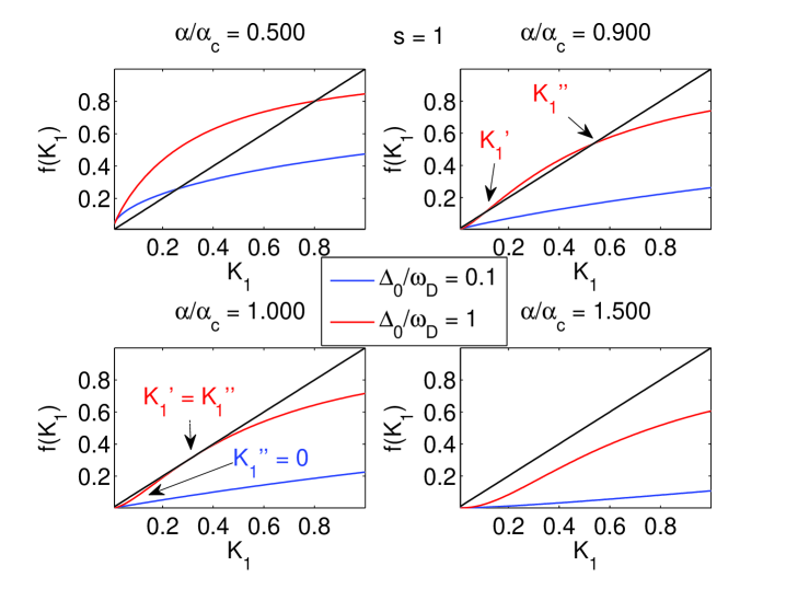
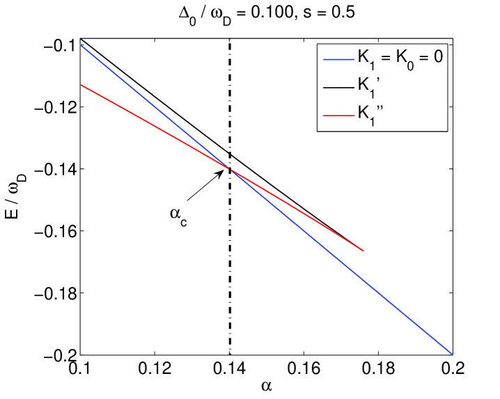
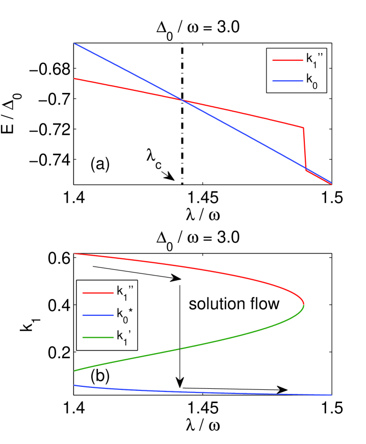
and $k_{0}=e^{-2(\lambda/\omega)^{2}}$. The above equation, in general, have three solutions $k_{0}*,k_{1}^{\prime}$, and $k_{1}^{\prime\prime}$ where $k_{0}*<k_{1}^{\prime}<k_{1}^{\prime\prime}$. Numerical analysis shows there exists a frequency threshold $\omega_{c}$, variational schemes fail only for $\omega<\omega_{c}$ at $\lambda=\lambda_{c}$, which is $\omega$-dependent. It turns out that, for $\omega>\omega_{c}$, the variational ground state is always stable, i.e., $E(k_{1})<E(k_{0})$, and the tunneling splitting $k_{1}\Delta_{0}$ decreases continuously with increasing $\lambda$. However, for $\omega<\omega_{c}$, the tunneling splitting shows a discontinuous jump as $\lambda$ approaching $\lambda_{c}$, at where the variational ground state becomes unstable. Figure 5 shows the variation of both the energy and tunneling splitting around the fail point. In fact, such a discontinuous jump was firstly reported in Ref. ss, and stated it as an artifact of the variational calculation. Our analysis shows clearly this artifact is due to the fail point of the variational scheme. Nevertheless, the discontinuous jump in the single mode case has some important difference from the discontinuous transition in the multi-mode case. First of all, the discontinuous jump does not exactly lead to a crossover from the delocalized to localized phases since both phases have non-zero tunneling splitting. The most important difference is that the transition is not from the variational ground state to the displaced-oscillator ground state, but to a state closed to it. This is because $k_{0}$ is not a solution of the self-consistent equation (32), a situation that is qualitatively different from the multi-mode case where $K_{0}=0$ is the trivial solution of self-consistent equation (12) in both the Ohmic and sub-Ohmic cases. Since the transition determined from the self-consistent equation can only happens between the solutions of this equation, the transition cannot be from the variational ground state to the displaced-oscillator ground state directly, nevertheless the difference becomes very small when $\omega/\Delta_{0}\leq 1/5$.

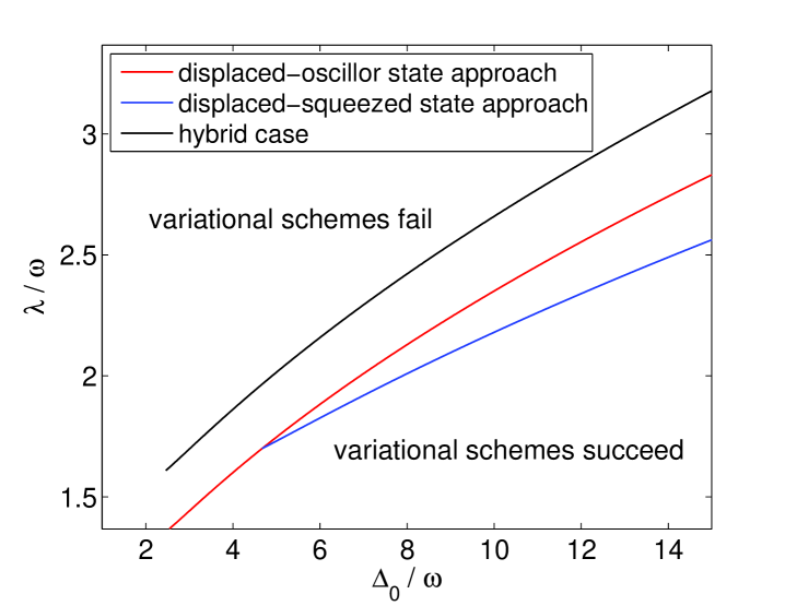
Fail points of other variational schemes can be analyzed in the same way. The situation is almost the same for all three variational schemes except the values of $\omega_{c}$ and the corresponding $\lambda_{c}$. Figure 6 shows the boundary lines of the fail points as a function of $\Delta_{0}/\omega$ and $\lambda/\omega$ for all the three variational schemes. As one can see from Fig. 6, all variational schemes fail in the low frequency and strong coupling regions.

It should be noted that the above analysis cannot be generalized directly to the case of $T\not=0$. This is because the system with a Hamiltonian given in Eq. (30) is not a true thermodynamical system. To perform the variational calculation as in the multi-mode case, one needs to include the environment as a “thermo-bath”, i.e., the effect of the environment is just to keep the single-mode system in thermodynamical equilibrium. Under this sense, we can do a variational calculation based on the DOS and the up-bound of the free energy in the present case is given by

where

and $k_{2}$ is determined by the self-consistent equation

Correspondingly, the up-bound of the free energy of the displaced-oscillator ground state is

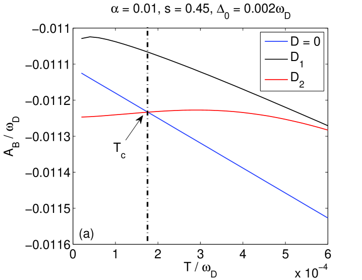
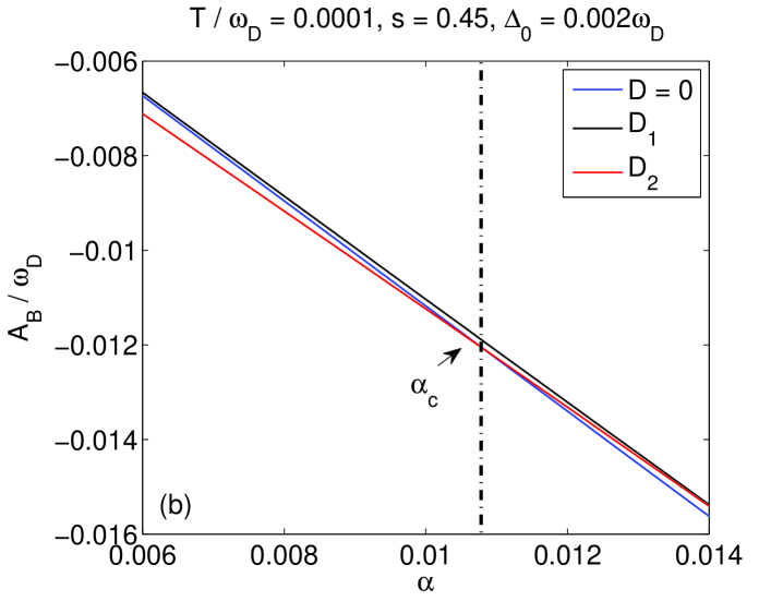
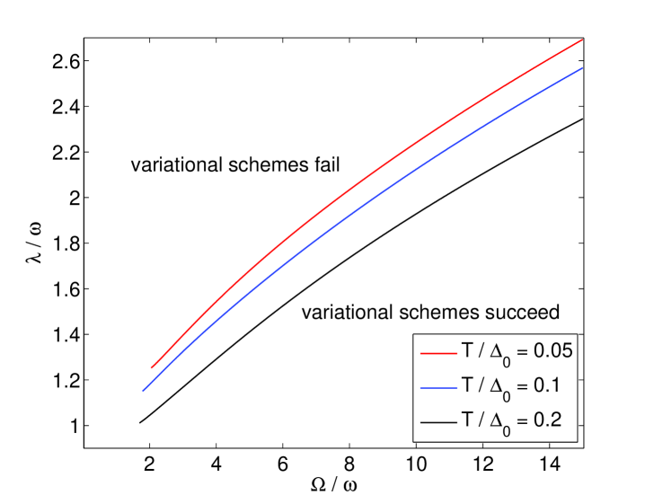
where $k_{3}=\exp\{-2(\lambda/\omega)^{2}\coth(\beta\omega/2)\}$. Using the above result, one can make analysis on the stability of variational thermodynamical ground state as before. As expected, it turns out that the situation is almost the same as in the case of $T=0$. There is a frequency threshold $\omega_{c}$. For $\omega>\omega_{c}$, we have $f_{a}<f_{0}$, i.e., variational thermodynamical ground state is always stable for all the coupling range and $k_{2}\Delta_{0}$ decreases continuously with increasing $\lambda$; however, for $\omega<\omega_{c}$, variational thermodynamical ground state becomes unstable as the coupling reaches some critical value $\lambda_{c}$ which is again $\omega$-dependent. Tunneling splitting shows a discontinuous jump when the fail point is reached. In the case of $T\not=0$, the fail point can be reached in another way; that is, for a given coupling $\lambda$, one can find that the variational scheme fails when temperature rises to some critical value $T_{c}$, at where tunneling splitting also shows a discontinuous jump. The boundary line of the fail point for the variational scheme based on the DOS in the case of $T\not=0$ is shown in Fig. 7. The boundary lowers down as the temperature increases, which implies that the variational scheme fails at a lower $\lambda_{c}$ as $T$ increases.

Why variational schemes fail in the low frequency region? Physically, in the high frequency region with $\omega/\Delta_{0}\gg 1$, the first term in Eq. (1) or (30) can be treated as a small perturbation, hence the DOS is a good trial ground state for the variational calculation; however, in the low frequency region with $\Delta_{0}/\omega\gg 1$, the DOS is not appropriate to serve as the trial ground state since the term $\frac{1}{2}\Delta_{0}\hat{\sigma}_{x}$ makes the main contribution in the single mode case. As one can see from the analysis presented in Ref. 4, in the low frequency region, the true ground state of the phonon bath in the single mode case is a combination of the two DOS with opposite displacement, i.e.,

where $g_{1,2}$ and $a$ are functions of $\lambda/\Delta_{0}$ and $\omega/\Delta_{0}$. Numerical analysis shows that $|\phi_{ph}\rangle$ gives a very accurate description for the phonon ground state in the low frequency region with strong couplings. Obviously, $|\phi_{ph}\rangle$ can be described by neither a DOS-like nor a DSS-like state, showing that both the DOS and DSS can not serve as the trial ground states in the low frequency region with strong couplings. As shown in Ref. 4, a variational scheme by taking a trial ground state as $|\phi_{ph}\rangle$ shows no discontinuous jump. We have made numerical analysis on the energy of the variational ground state based on $|\phi_{ph}\rangle$, which is found to be always stable against the displaced-oscillator ground state in all the coupling regime. This result clearly shows that the failure of the variational scheme is due to the invalid trial ground state in the low frequency regions. The above analysis provides the answer to why the variational schemes based on both the DOS and DSS always fail in low frequency region with strong couplings.

It should be noted that the low frequency modes play important roles in the localized transition. As one can see from the self-consistent equations (12) or (27), the integral can be divided into two parts like, $\int_{0}^{\omega_{D}}\rightarrow\int_{0}^{\omega_{c}}+\int_{\omega_{c}}^{\omega_{D}}$, without the contribution of the low frequency modes lie in $(0,\omega_{c})$, there is no localization for any finite $\alpha$. In other words, it is the low frequency modes lead to localization. The failure of the variational schemes in the low frequency regions implies that the variational calculations fail to take account of the contribution of the low frequency modes to the localization, making the predicted localization in question.

To the first order approximation (i.e., by omitting the cooperative effect between different phonon modes), the result of multi-mode case can be considered as a combination of all the phonon modes lie in $(0,\omega_{D})$ with a frequency-dependent weight. Generally speaking, the parameter $s$ in the spectral function $J(\omega)$ determines the weight, while for counting the contribution of the phonon modes that have fail point; the parameter $\Delta_{0}/\omega_{D}$ is therefore important and the boundary $\omega_{c}$ is in scale of $\Delta_{0}$ as shown in Fig. 6. Let us take the variational scheme based on the DOS as an example. Giving that $\Delta_{0}/\omega_{D}=0.1$, one can see from Fig. 6 that $\omega_{c}/\Delta_{0}\simeq 1/3$, which implies that the frequency modes with frequency $0<\omega<0.03\omega_{D}$ have fail points, i.e., about 3 percent phonon modes have fail points. However, if one takes $\Delta_{0}/\omega_{D}=1$ as shown in Fig. 1, then there are about 30 percent phonon modes have fail points. This result shows that the population of the phonon modes having fail points is directly controlled by the value of $\Delta_{0}/\omega_{D}$. Now we know that only the phonon modes have fail points will contribute a discontinuous jump of the tunneling splitting as the coupling reached the critical point. In the Ohmic case with $\Delta_{0}/\omega_{D}\ll 1$, the discontinuous contribution of the low frequency modes at the fail point is overwhelmed by the continuous contribution from the high frequency modes, leading to a continuous transition; however, as $\Delta_{0}/\omega_{D}$ increases to some larger value (say, 0.5 in the DOS case), the increasing population of phonon modes having fail points leads to an observable discontinuous contribution and the transition behavior turns to discontinuous. In the sub-Ohmic case, the weight of the low frequency modes increases so that the discontinuous contribution from phonon modes having fail points becomes observable even when $\Delta_{0}/\omega_{D}\ll 1$, hence the transition is always discontinuous. However, for the same reason, one can easily predict that the discontinuous transitions will be unapparent when $\Delta_{0}/\omega_{D}$ becomes too small. It should be noted that the discontinuous transition in the sub-Ohmic case is just due to the fail point of the variational schemes, not the true crossover behavior of the model since it is not expected to be seen in the NRG or DMRG calculation.bulla ; b1 ; wh1

The above analysis can be generalized to the case of $T\not=0$. It has been shown that the transition behavior predicted by the variational calculations at $T\not=0$ is discontinuous for $0<s<2$.ch The key point is to understand why the discontinuous transition behavior is extended to the super-Ohmic case. By comparing the two self-consistent equations (12) for $T=0$ and (27) for $T\not=0$, at $T\not=0$, the spectral function is effectively modified as $J(\omega)\coth(\beta\omega/2)$, i.e., an extra factor $\coth(\beta\omega/2)$ appears in numerator of the integrand. It is obvious that, $\coth(\beta\omega/2)\propto 1/\omega$ as $\omega\rightarrow 0$, which implies that, in the low frequency regions, $J(\omega)\coth(\beta\omega/2)\propto\omega^{s-1}$. In other words, the extra factor $\coth(\beta\omega/2)$ seriously increases the weight of the low frequency modes having fail points, resulting in a discontinuous transition behavior even in the super-Ohmic case.

Mathematical analysis on the self-consistent equations derived from the variational condition at both $T=0$ and $T\not=0$ shows there exists a universal $s_{c}$ for all the variational schemes, the predicted transition is always discontinuous for $0<s<s_{c}$, a continuous transition can only be found when $s=s_{c}$ with $\Delta_{0}/\omega_{D}\ll 1$. It was found that $s_{c}=1$ for $T=0$ and $s_{c}=2$ for $T\not=0$.ch The above analysis clearly shows that the predicted transition behavior depends on both the weight and the population of the low frequency modes.