Var
\coltauthor\NameMax Dabagia \Emailmaxdabagia@gatech.edu
\addrSchool of Computer Science, Georgia Tech
and \NameChristos H. Papadimitriou \Emailchristos@columbia.edu
\addrDepartment of Computer Science, Columbia University
and \NameSantosh S. Vempala \Emailvempala@gatech.edu
\addrSchool of Computer Science, Georgia Tech
Assemblies of Neurons Learn to Classify Well-Separated Distributions
Abstract
An assembly is a large population of neurons whose synchronous firing is hypothesized to represent a memory, concept, word, and other cognitive categories. Assemblies are believed to provide a bridge between high-level cognitive phenomena and low-level neural activity. Recently, a computational system called the Assembly Calculus (AC), with a repertoire of biologically plausible operations on assemblies, has been shown capable of simulating arbitrary space-bounded computation, but also of simulating complex cognitive phenomena such as language, reasoning, and planning. However, the mechanism whereby assemblies can mediate learning has not been known. Here we present such a mechanism, and prove rigorously that, for simple classification problems defined on distributions of labeled assemblies, a new assembly representing each class can be reliably formed in response to a few stimuli from the class; this assembly is henceforth reliably recalled in response to new stimuli from the same class. Furthermore, such class assemblies will be distinguishable as long as the respective classes are reasonably separated — for example, when they are clusters of similar assemblies, or more generally separable with margin by a linear threshold function. To prove these results, we draw on random graph theory with dynamic edge weights to estimate sequences of activated vertices, yielding strong generalizations of previous calculations and theorems in this field over the past five years. These theorems are backed up by experiments demonstrating the successful formation of assemblies which represent concept classes on synthetic data drawn from such distributions, and also on MNIST, which lends itself to classification through one assembly per digit. Seen as a learning algorithm, this mechanism is entirely online, generalizes from very few samples, and requires only mild supervision — all key attributes of learning in a model of the brain. We argue that this learning mechanism, supported by separate sensory pre-processing mechanisms for extracting attributes, such as edges or phonemes, from real world data, can be the basis of biological learning in cortex.
keywords:
List of keywords1 Introduction
The brain has been a productive source of inspiration for AI, from the perceptron and the neocognitron to deep neural nets. Machine learning has since advanced to dizzying heights of analytical understanding and practical success, but the study of the brain has lagged behind in one important dimension: After half a century of intensive effort by neuroscientists (both computational and experimental), and despite great advances in our understanding of the brain at the level of neurons, synapses, and neural circuits, we still have no plausible mechanism for explaining intelligence, that is, the brain’s performance in planning, decision-making, language, etc. As Nobel laureate Richard Axel put it, “we have no logic for translating neural activity into thought and action” (Axel, 2018).
Recently, a high-level computational framework was developed with the explicit goal to fill this gap: the Assembly Calculus (AC) (Papadimitriou et al., 2020), a computational model whose basic data type is the assembly of neurons. Assemblies, called “the alphabet of the brain” (Buzsáki, 2019), are large sets of neurons whose simultaneous excitation is tantamount to the subject’s thinking of an object, idea, episode, or word (see Piantadosi et al. (2016)). Dating back to the birth of neuroscience, the “million-fold democracy” by which groups of neurons act collectively without central control was first proposed by Sherrington (1906) and was the empirical phenomenon that Hebb attempted to explain with his theory of plasticity (Hebb, 1949). Assemblies are initially created to record memories of external stimuli (Quiroga, 2016), and are believed to be subsequently recalled, copied, altered, and manipulated in the non-sensory brain (Piantadosi et al., 2012; Buzsáki, 2010). The Assembly Calculus provides a repertoire of operations for such manipulation, namely project, reciprocal-project, associate, pattern-complete, and merge encompassing a complete computational system. Since the Assembly Calculus is, to our knowledge, the only extant computational system whose purpose is to bridge the gap identified by Axel in the above quote (Axel, 2018), it is of great interest to establish that complex cognitive functions can be plausibly expressed in it. Indeed, significance progress has been made over the past year, see for example Mitropolsky et al. (2021) for a parser of English and d’Amore et al. (2021) for a program mediating planning in the blocks world, both written in the AC programming system. Yet despite these recent advances, one fundamental question is left unanswered: If the Assembly Calculus is a meaningful abstraction of cognition and intelligence, why does it not have a learn command? How can the brain learn through assembly representations?
This is the question addressed and answered in this paper. As assembly operations are a new learning framework and device, one has to start from the most basic questions: Can this model classify assembly-encoded stimuli that are separated through clustering, or by half spaces? Recall that learning linear thresholds is a theoretical cornerstone of supervised learning, leading to a legion of fundamental algorithms: Perceptron, Winnow, multiplicative weights, isotron, kernels and SVMs, and many variants of gradient descent.
Following Papadimitriou et al. (2020), we model the brain as a directed graph of excitatory neurons with dynamic edge weights (due to plasticity). The brain is subdivided into areas, for simplicity each containing neurons connected through a random directed graph (Erdős and Rényi, 1960). Certain ordered pairs of areas are also connected, through random bipartite graphs. We assume that neurons fire in discrete time steps. At each time step, each neuron in a brain area will fire if its synaptic input from the firings of the previous step is among the top highest out of the neurons in its brain area. This selection process is called -cap, and is an abstraction of the process of inhibition in the brain, in which a separate population of inhibitory neurons is induced to fire by the firing of excitatory neurons in the area, and through negatively-weighted connections prevents all but the most stimulated excitatory neurons from firing. Synaptic weights are altered via Hebbian plasticity and homeostasis (see Section 2 for a full description). In this stylized mathematical model, reasonably consistent with what is known about the brain, it has been shown that the operations of the Assembly Calculus converge and work as specified (with high probability relative to the underlying random graphs). These results have also been replicated by simulations in the model above, and also in more biologically realistic networks of spiking neurons (see Legenstein et al. (2018); Papadimitriou et al. (2020)). In this paper we develop, in the same model, mechanisms for learning to classify well-separated classes of stimuli, including clustered distributions and linear threshold functions with margin. Moreover, considering that the ability to learn from few examples, and with mild supervision, are crucial characteristics of any brain-like learning algorithm, we show that learning with assemblies does both quite naturally.
2 A mathematical model of the brain
Here we outline the basics of the model in Papadimitriou et al. (2020). There are a finite number of brain areas, denoted (but in this paper, we will only need one brain area where learning happens, plus another area where the stimuli are presented). Each area is a random directed graph with nodes called neurons with each directed edge present independently with probability (for simplicity, we take and to be the same across areas). Some ordered pairs of brain areas are also connected by random bipartite graphs, with the same connection probability . Importantly, each area may be inhibited, which means that its neurons cannot fire; the status of the areas is determined by explicit inhibit/disinhibit commands of the AC. 111The brain’s neuromodulatory systems (Jones, 2003; Harris and Thiele, 2011) are plausible candidates to implement these mechanisms. This defines a large random graph with nodes and a number of directed edges which is in expectation , where is the number of pairs of areas that are connected. Each edge in this graph, called a synapse, has a dynamic non-negative weight , initially .
This framework gives rise to a discrete-time dynamical system, as follows: The state of the system at any time step consists of (a) a bit for each area , inh, initially , denoting whether the area is inhibited; (b) a bit for each neuron , fires, denoting whether spikes at time (zero if the area of has inh); and (c) the weights of all synapses , initially one.
The state transition of the dynamical system is as follows: For each neuron in area with inh (see the next paragraph for how inh is determined), define its synaptic input at time ,
For each in area with inh, we set fires iff is among the neurons in its area that have highest SI (breaking ties arbitrarily). This is the -cap operation, a basic ingredient of the AC framework, modeling the inhibitory/excitatory balance of a brain area.222Binas et al. (2014) showed rigorously how a -cap dynamic could be emerge in a network of excitatory and inhibitory neurons. As for the synaptic weights,
That is, if fires at time and fires at time , Hebbian plasticity dictates that be increased by a factor of at time . So that the weights do not grow unlimited, a homeostasis process renormalizes, at a slower time scale, the sum of weights along the incoming synapses of each neuron (see Davis (2006) and Turrigiano (2011) for reviews of this mechanism in the brain).
Finally, the AC is a computational system driving the dynamical system by executing commands at each time step (like a programming language driving the physical system that is the computer’s hardware). The AC commands (dis)inhibit change the inhibition status of an area at time ; and the command fire, where is the name of an assembly (defined next) in a disinhibited area, overrides the selection by -cap, and causes the neurons of assembly to fire at time .
An assembly is a highly interconnected (in terms of both number of synapses and their weights) set of neurons in an area encoding a real world entity. Initially, assembly-like representations exist only in a special sensory area, as representations of perceived real-world entities such as a heard (or read) word. Assemblies in the remaining, non-sensory areas are an emergent behavior of the system, copied and re-copied, merged, associated, etc., through further commands of the AC. This is how the model is able to simulate arbitrary space bounded computations (Papadimitriou et al., 2020). The most basic such command is project, which, starting from an assembly in area , creates in area (where there is connectivity from to ) a new assembly , which has strong synaptic connectivity from and which will henceforth fire every time fires in the previous step, and is not inhibited. This command entails disinhibiting the areas , and then firing (the neurons in) assembly for the next time steps. It was shown by Papadimitriou and Vempala (2019) that, with high probability, after a small number of steps, a stable assembly in will emerge, which is densely intraconnected and has high connectivity from . The mechanism achieving this convergence involves synaptic input from , which creates an initial set of firing neurons in , which then evolves to through sustained synaptic input from and recurrent input from , while these two effects are further enhanced by plasticity.
Incidentally, this convergence proof (see Legenstein (2018); Papadimitriou and Vempala (2019); Papadimitriou et al. (2020) for a sequence of sharpened versions of this proof over the past years) is the most mathematically sophisticated contribution of this theory to date. The theorems of the present paper can be seen as substantial generalizations of that result: Whereas in previous work an assembly is formed as a copy of one stimulus firing repeatedly (memorization), so that this new assembly will henceforth fire whenever the same stimulus us presented again, in this paper we show rigorously that an assembly will be formed in response to the sequential firing of many stimuli, all drown from the same distribution (generalization), and the formed assembly will fire reliably every time another stimulus from the same distribution is presented.
The key parameters of our model are , and . Intended values for the brain are , but in our simulations we have also had success on a much smaller scale, with . is an important parameter, in that adequately large values of guarantee the convergence of the AC operations. For a publicly available simulator of the Assembly Calculus (in which the Learning System below can be readily implemented) see \urlhttp://brain.cc.gatech.edu.
The learning mechanism.
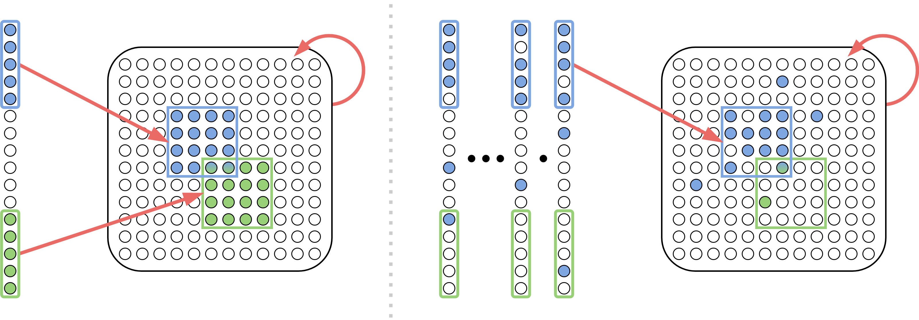
For the purpose of demonstrating learning within the framework of AC, we consider the specific setting described below. First, there is a special area, called the sensory area, in which training and testing data are encoded as assembly-like representations called stimuli. There is only one other brain area (besides the sensory area), and that is where learning happens, through the formation of assemblies in response to sequences of stimuli.
A stimulus is a set of about neurons firing simultaneously (“presented”) in the sensory area. Note that, exceptionally in the sensory area, a number of neurons that is a little different from may fire at a step. A stimulus class is a distribution over stimuli, defined by three parameters: two scalars , and a set of neurons in the sensory area. To generate a stimulus in the class , each neuron is chosen with probability , while for each , the probability of choosing neuron is . It follows immediately that, in expectation, an fraction of the neurons in the stimulus core are set to and the number of neurons outside the core that are set to is also .
The presentation of a sequence of stimuli from a class in the sensory area evokes in the learning system a response , a distribution over assemblies in the brain area. We show that, as a consequence of plasticity and -cap, this distribution will be highly concentrated, in the following sense: Consider the set of all assemblies that have positive probability in . Then the numbers of neurons in both the intersection , called the core of and the union are close to , in particular and respectively.333The larger the plasticity, the closer these two values are (see Papadimitriou and Vempala (2019), Fig. 2). In other words, neurons in fire far more often on average than neurons in .
Finally, our learning protocol is this: Beginning with the brain area at rest, stimuli are repeatedly sampled from the class, and made to fire. After a small number of training samples, the brain area returns to rest, and then the same procedure is repeated for the next stimulus class, and so on. Then testing stimuli are presented in random order to test the extent of learning. (see Algorithm 1 in an AC-derived programming language.)
The learning mechanism. ( denotes the brain area.)
\KwIna set of stimulus classes ;
\KwOutA set of assemblies in the brain area encoding these classes
\ForEach stimulus class
inh
\ForEach time step
Sample and fire
inh
That is, we sample stimuli from each class, fire each to cause synaptic input in the brain area, and after the th sample has fired we record the assembly which has been formed in the brain area. This is the representation for this class.
Related work
There are numerous learning models in the neuroscience literature. In a variation of the model we consider here, Rangamani and Gandhi (2020) have considered supervised learning of Boolean functions using assemblies of neurons, by setting up separate brain areas for each label value. Amongst other systems with rigorous guarantees, assemblies are superficially similar to the “items” of Valiant’s neuroidal model (Valiant, 1994), in which supervised learning experiments have been conducted (Valiant, 2000; Feldman and Valiant, 2009), where an output neuron is clamped to the correct label value, while the network weights are updated under the model. The neuroidal model is considerably more powerful than ours, allowing for arbitrary state changes of neurons and synapses; in contrast, our assemblies rely on only two biologically sound mechanisms, plasticity and inhibition.
Hopfield nets (Hopfield, 1982) are recurrent networks of neurons with symmetric connection weights which will converge to a memorized state from a sufficiently similar one, when properly trained using a local and incremental update rule. In contrast, the memorized states our model produces (which we call assemblies) emerge through plasticity and randomization from the structure of a random directed network, whose weights are asymmetric and nonnegative, and in which inhibition — not the sign of total input — selects which neurons will fire.
Stronger learning mechanisms have recently been proposed. Inspired by the success of deep learning, a large body of work has shown that cleverly laid-out microcircuits of neurons can approximate backpropagation to perform gradient descent (Lillicrap et al., 2016; Sacramento et al., 2017; Guerguiev et al., 2017; Sacramento et al., 2018; Whittington and Bogacz, 2019; Lillicrap et al., 2020). These models rely crucially on novel types of neural circuits which, although biologically possible, are not presently known or hypothesized in neurobiology, nor are they proposed as a theory of the way the brain works. These models are capable of matching the performance of deep networks on many tasks, which are more complex than the simple, classical learning problems we consider here. The difference between this work and ours is, again, that here we are showing that learning arises naturally from well-understood mechanisms in the brain, in the context of the assembly calculus.
3 Results
Very few stimuli sampled from an input distribution are activated sequentially at the sensory area. The only form of supervision required is that all training samples from a given class are presented consecutively. Plasticity and inhibition alone ensure that, in response to this activation, an assembly will be formed for each class, and that this same assembly will be recalled at testing upon presentation of other samples from the same distribution. In other words, learning happens. And in fact, despite all these limitations, we show that the device is an efficient learner of interesting concept classes.
Our first theorem is about the creation of an assembly in response to inputs from a stimulus class. This is a generalization of a theorem from Papadimitriou and Vempala (2019), where the input stimulus was held constant; here the input is a stream of random samples from the same stimulus class. Like all our results, it is a statement holding with high probability (WHP), where the underlying random event is the random graph and the random samples. When sampled stimuli fire, the assembly in the brain area changes. The neurons participating in the current assembly (those whose synaptic input from the previous step is among the highest) are called the current winners. A first-time winner is a current winner that participated in no previous assembly (for the current stimulus class).
Theorem 3.1 (Creation).
Consider a stimulus class projected to a brain area. Assume that
Then WHP no first-time winners will enter the cap after rounds, and moreover the total number of winners can be bounded as
Remark 3.2.
The theorem implies that for a small constant , it suffices to have plasticity parameter
Our second theorem is about recall for a single assembly, when a new stimulus from the same class is presented. We assume that examples from an an assembly class have been presented, and a response assembly encoding this class has been created, by the previous theorem.
Theorem 3.3 (Recall).
WHP over the stimulus class, the set firing in response to a test assembly from the class will overlap by a fraction of at least , i.e.
The proof entails showing that the average weight of incoming connections to a neuron in from neurons in is at least
Our third theorem is about the creation of a second assembly corresponding to a second stimulus class. This can easily be extended to many classes and assemblies. As in the previous theorem, we assume that examples from assembly class have been presented, and has been created. Then we introduce , a second stimulus class, with , and present samples to induce a series of caps, , with as their union.
Theorem 3.4 (Multiple Assemblies).
The total support of can be bounded WHP as
Moreover, WHP, the overlap in the core sets and will preserve the overlap of the stimulus classes, so that .
This time the proof relies on the fact that the average weight of incoming connections to a neuron in is upper-bounded by
Our fourth theorem is about classification after the creation of multiple assemblies, and shows that random stimuli from any class are mapped to their corresponding assembly. We state it here for two stimuli classes, but again it is extended to several. We assume that stimulus classes and overlap in their core sets by a fraction of , and that they have been projected to form a distribution of assemblies and , respectively.
Theorem 3.5 (Classification).
If a random stimulus chosen from a particular class (WLOG, say ) fires to cause a set of learning area neurons to fire, then WHP over the stimulus class the fraction of neurons in the cap and in will be at least
where is a lower bound on the average weight of incoming connections to a neuron in (resp. ) from neurons in (resp. ).
Taken together, the above results guarantee that this mechanism can learn to classify well-separated distributions, where each distribution has a constant fraction of its nonzero coordinates in a subset of input coordinates. The process is naturally interpretable: an assembly is created for each distribution, so that random stimuli are mapped to their corresponding assemblies, and the assemblies for different distributions overlap in no more than the core subsets of their corresponding distributions.
Finally, we consider the setting where the labeling function is a linear threshold function, parameterized by an arbitrary nonnegative vector and margin . We will create a single assembly to represent examples on one side of the threshold, i.e. those for which . We define denote the distribution of these examples, where each coordinate is an independent Bernoulli variable with mean , and define to be the distribution of negative examples, where each coordinate is again an independent Bernoulli variable yet now all identically distributed with mean . (Note that the support of the positive and negative distributions is the same; there is a small probability of drawing a positive example from the negative distribution, or vice versa.) To serve as a classifier, a fraction of neurons in the assembly must be guaranteed to fire for a positive example, and a fraction guaranteed not to fire for a negative one. A test example is then classified as positive if at least a fraction of neurons in the assembly fire (for ), and negative otherwise. The last theorem shows that this can in fact be done with high probability, as long as the normal vector of the linear threshold is neither too dense nor too sparse. Additionally, we assume synapses are subject to homeostasis in between training and evaluation; that is, all of the incoming weights to a neuron are normalized to sum to 1.
Theorem 3.6 (Learning Linear Thresholds).
Let be a nonnegative vector normalized to be of unit Euclidean length (). Assume that and
Then, sequentially presenting samples drawn at random from forms an assembly that correctly separates from : with probability a randomly drawn example from will result in a cap which overlaps at least neurons in , and an example from will create a cap which overlaps no more than neurons in .
Remark 3.7.
The bound on leads to two regimes of particular interest: In the first,
and , which is similar to the plasticity parameter required for a fixed stimulus (Papadimitriou and Vempala, 2019) or stimulus classes; in the second, is a constant, and
Remark 3.8.
We can ensure that the number of neurons outside of for a positive example or in for a negative example are both with small overhead444i.e. increasing the plasticity constant by a factor of , so that plasticity can be active during the classification phase.
Since our focus in this paper is on highlighting the brain-like aspects of this learning mechanism, we emphasize stimulus classes as a case of particular interest, as they are a probabilistic generalization of the single stimuli considered in Papadimitriou and Vempala (2019). Linear threshold functions are an equally natural way to generalize a single -sparse stimulus, say ; all the 0/1 points on the positive side of the threshold have at least an fraction of the neurons of the stimulus active.
Finally, reading the output of the device by the Assembly Calculus is simple: Add a readout area to the two areas so far (stimulus and learning), and project to this area one of the assemblies formed in the learning area for each stimulus class. The assembly in the learning area that fires in response to a test sample will cause the assembly in the readout area corresponding to the class to fire, and this can be sensed through the readout operation of the AC.
Proof overview.
The proofs of all five theorems can be found in the Appendix. The proofs hinge on showing that large numbers of certain neurons of interest will be included in the cap on a particular round — or excluded from it. More specifically:
-
•
To create an assembly, the sequence of caps should converge to the assembly’s core set. In other words, WHP an increasing fraction of the neurons selected by the cap in a particular step will also be selected at the next one.
-
•
For recall, a large fraction of the assembly should fire (i.e. be included in the cap) when presented with an example from the class.
-
•
To differentiate stimuli (i.e. classify), we need to ensure that a large fraction of the correct assembly will fire, while no more than a small fraction of the other assemblies do.
Following Papadimitriou and Vempala (2019), we observe that if the probability of a neuron having input at least is no more than , then no more than an fraction of the cohort of neurons will have input exceeding (with constant probability). By approximating the total input to a neuron as Gaussian and using well-known bounds on Gaussian tail probabilities, we can solve for , which gives an explicit input threshold neurons must surpass to make a particular cap. Then, we argue that the advantage conferred by plasticity, combined with the similarity of examples from the same class, gives the neurons of interest enough of an advantage that the input to all but a small constant fraction will exceed the threshold.
4 Experiments
The learning algorithm has been run on both synthetic and real-world datasets, as illustrated in the figures below. Code for experiments is available at \urlhttps://github.com/mdabagia/learning-with-assemblies.
Beyond the basic method of presenting a few examples from the same class and allowing plasticity to alter synaptic weights, the training procedure is slightly different for each of the concept classes (stimulus classes, linearly-separated, and MNIST digits). In each case, we renormalize the incoming weights of each neuron to sum to one after concluding the presentation of each class, and classification is performed on top of the learned assemblies by predicting the class corresponding to the assembly with the most neurons on.
-
•
For stimulus classes, we estimate the assembly for each class as composed of the neurons which fired in response to the last training example, which in practice are the same as those most likely to fire for a random test example.
-
•
For a linear threshold, we only present positive examples, and thus only form an assembly for one class. As with stimulus classes, the neurons in the assembly can be estimated by the last training cap or by averaging over test examples. We classify by comparing against a fixed threshold, generally half the cap size.
Additionally, it is important to set the plasticity parameter () large enough that assemblies are reliably formed. We had success with for stimulus classes and for linear thresholds.
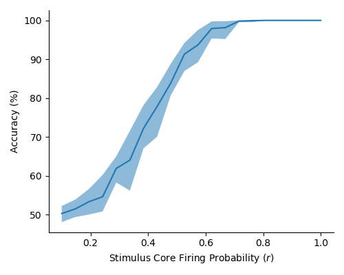
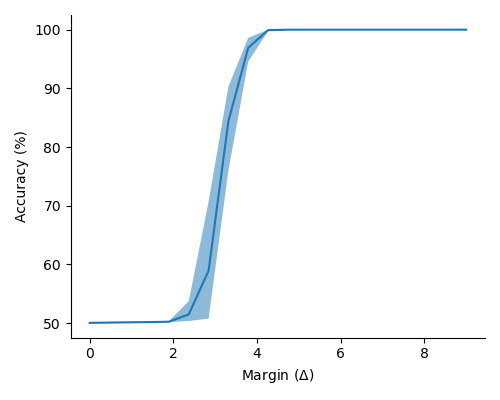
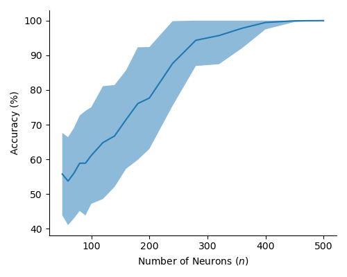
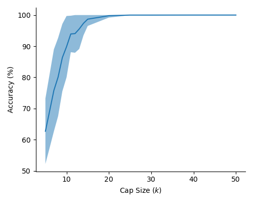
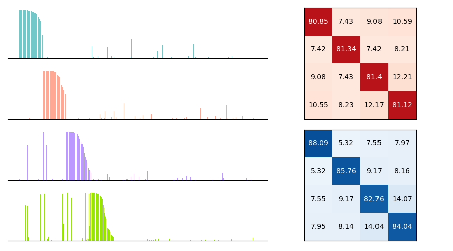
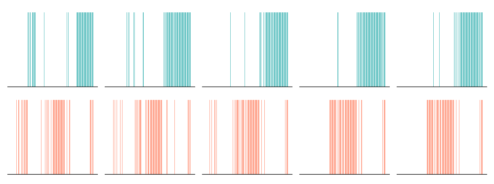
In Figure 2 (a) & (b), we demonstrate learning of two stimulus classes, while in Figure 2 (c) & (d), we demonstrate the result of learning a well-separated linear threshold function with assemblies. Both had perfect accuracy. Additionally, assemblies readily generalize to a larger number of classes (see Figure 6 in the appendix). We also recorded sharp threshold transitions in classification performance as the key parameters of the model are varied (see Figures 3 & 4).


There are a number of possible extensions to the simplest strategy, where within a single brain region we learn an assembly for each concept class and classify based on which assembly is most activated in response to an example. We compared the performance of various classification models on MNIST as the number of features increases. The high-level model is to extract a certain number of features using one of the five different methods, and then find the best linear classifier (of the training data) on these features to measure performance (on the test data). The five different feature extractors are:
-
•
Linear features. Each feature’s weights are sampled i.i.d. from a Gaussian with standard deviation .
-
•
Nonlinear features. Each feature is a binary neuron: it has i.i.d. Bernoulli weights, and ‘fires’ (has output , otherwise ) if its total input exceeds the expected input ().
-
•
Large area assembly features. In a single brain area of size with cap size , we attempt to form an assembly for each class. The area sees a sequence of examples from each class, with homeostasis applied after each class. Weights are updated according to Hebbian plasticity with . Additionally, we apply a negative bias: A neuron which has fired for a given class is heavily penalized against firing for subsequent classes.
-
•
’Random’ assembly features. For a total of features, we create different areas of neurons each, with cap size . We then repeat the large area training procedure above in each area, with the order of the presentation of classes randomized for each area.
-
•
’Split’ assembly features: For a total of features, we create different areas of neurons each, with cap size . Area sees a sequence of examples from class . Weights are updated according to Hebbian plasticity, and homeostasis is applied after training.
After extracting features, we train the linear classification layer to minimize cross-entropy loss on the standard MNIST training set ( images) and finally test on the full test set ( images).
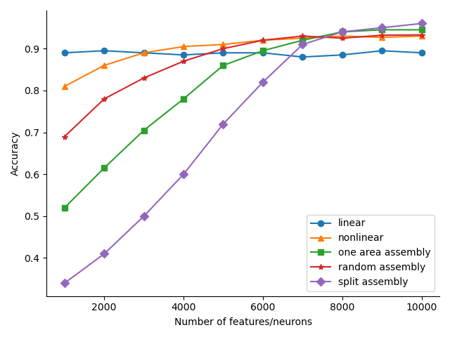
The results as the total number of features ranges from to is shown in Fig. 5. ’Split’ assembly features are ultimately the best of the five, with ’split’ features achieving accuracy with features. However, nonlinear features outperform ’split’ and large-area features and match ’random’ assembly features when the number of features is less than . For reference, the linear classifier gets to , while a two-layer neural network with width trained end-to-end gets to .
Going further, one could even create a hierarchy of brain areas, so that the areas in the first “layer” all project to a higher-level area, in hopes of forming assemblies for each digit in the higher-level area which are more robust. In this paper, our goal was to highlight the potential to form useful representations of a classification dataset using assemblies, and so we concentrated on a single layer of brain areas with a very simple classification layer on top. It will be interesting to explore what is possible with more complex architectures.
5 Discussion
Assemblies are widely believed to be involved in cognitive phenomena, and the AC provides evidence of their computational aptitude. Here we have made the first steps towards understanding how learning can happen in assemblies. Normally, an assembly is associated with a stimulus, such as Grandma. We have shown that this can be extended to a distribution over stimuli. Furthermore, for a wide range of model parameters, distinct assemblies can be formed for multiple stimulus classes in a single brain area, so long as the classes are reasonably differentiated.
A model of the brain at this level of abstraction should allow for the kind of classification that the brain does effortlessly — e.g., the mechanism that enables us to understand that individual frames in a video of an object depict the same object. With this in mind, the learning algorithm we present is remarkably parsimonious: it generalizes from a handful of examples which are seen only once, and requires no outside control or supervision other than ensuring multiple samples from the same concept class are presented in succession (and this latter requirement could be relaxed in a more complex architecture which channels stimuli from different classes). Finally, even though our results are framed within the Assembly Calculus and the underlying brain model, we note that they have implications far beyond this realm. In particular, they suggest that any recurrent neural network, equipped with the mechanisms of plasticity and inhibition, will naturally form an assembly-like group of neurons to represent similar patterns of stimuli.
But of course, many questions remain. In this first step we considered a single brain area — whereas it is known that assemblies draw their computational power from the interaction, through the AC, among many areas. We believe that a more general architecture encompassing a hierarchy of interconnected brain areas, where the assemblies in one area act like stimulus classes for others, can succeed in learning more complex tasks — and even within a single brain area improvements can result from optimizing the various parameters, something that we have not tried yet.
In another direction, here we only considered Hebbian plasticity, the simplest and most well-understood mechanism for synaptic changes. Evidence is mounting in experimental neuroscience that the range of plasticity mechanisms is far more diverse (Magee and Grienberger, 2020), and in fact it has been demonstrated recently (Payeur et al., 2021) that more complex rules are sufficient to learn harder tasks. Which plasticity rules make learning by assemblies more powerful?
We showed that assemblies can learn nonnegative linear threshold functions with sufficiently large margins. Experimental results suggest that the requirement of nonnegativity is a limitation of our proof technique, as empirically assemblies readily learn arbitrary linear threshold functions (with margin). What other concept classes can assemblies provably learn? We know from support vector machines that linear threshold functions can be the basis of far more sophisticated learning when their input is pre-processed in specific ways, while the celebrated results of Rahimi and Recht (2007) demonstrated that certain families of random nonlinear features can approximate sophisticated kernels quite well. What would constitute a kernel in the context of assemblies? The sensory areas of the cortex (of which the visual cortex is the best studied example) do pre-process sensory inputs extracting features such as edges, colors, and motions. Presumably learning by the non-sensory brain — which is our focus here — operates on the output of such pre-processing. We believe that studying the implementation of kernels in cortex is a very promising direction for discovering powerful learning mechanisms in the brain based on assemblies.
We thank Shivam Garg, Chris Jung, and Mirabel Reid for helpful discussions. MD is supported by an NSF Graduate Research Fellowship. SV is supported in part by NSF awards CCF-1909756, CCF-2007443 and CCF-2134105. CP is supported by NSF Awards CCF-1763970 and CCF-1910700, and by a research contract with Softbank.
References
- Axel (2018) Richard Axel. Q & A. Neuron, 99:1110–1112, 2018.
- Binas et al. (2014) Jonathan Binas, Ueli Rutishauser, Giacomo Indiveri, and Michael Pfeiffer. Learning and stabilization of winner-take-all dynamics through interacting excitatory and inhibitory plasticity. Frontiers in computational neuroscience, 8:68, 2014.
- Buzsáki (2010) György Buzsáki. Neural syntax: cell assemblies, synapsembles, and readers. Neuron, 68(3), 2010.
- Buzsáki (2019) György Buzsáki. The Brain from Inside Out. Oxford University Press, 2019.
- d’Amore et al. (2021) Francesco d’Amore, Daniel Mitropolsky, Pierluigi Crescenzi, Emanuele Natale, and Christos H Papadimitriou. Planning with biological neurons and synapses. arXiv preprint arXiv:2112.08186, 2021.
- Davis (2006) Graeme W Davis. Homeostatic control of neural activity: from phenomenology to molecular design. Annu. Rev. Neurosci., 29:307–323, 2006.
- Erdős and Rényi (1960) Paul Erdős and Alfréd Rényi. On the evolution of random graphs. Publ. Math. Inst. Hung. Acad. Sci, 5(1):17–60, 1960.
- Feldman and Valiant (2009) Vitaly Feldman and Leslie G. Valiant. Experience-induced neural circuits that achieve high capacity. Neural Computation, 21(10):2715–2754, 2009. 10.1162/neco.2009.08-08-851.
- Guerguiev et al. (2017) Jordan Guerguiev, Timothy P Lillicrap, and Blake A Richards. Towards deep learning with segregated dendrites. ELife, 6:e22901, 2017.
- Harris and Thiele (2011) Kenneth D Harris and Alexander Thiele. Cortical state and attention. Nature reviews neuroscience, 12(9):509–523, 2011.
- Hebb (1949) Donald Olding Hebb. The organization of behavior: A neuropsychological theory. Wiley, New York, 1949.
- Hopfield (1982) John J Hopfield. Neural networks and physical systems with emergent collective computational abilities. Proceedings of the national academy of sciences, 79(8):2554–2558, 1982.
- Jones (2003) Barbara E Jones. Arousal systems. Front Biosci, 8(5):438–51, 2003.
- Legenstein et al. (2018) R. Legenstein, W. Maass, C. H. Papadimitriou, and S. S. Vempala. Long-term memory and the densest k-subgraph problem. In Proc. of 9th Innovations in Theoretical Computer Science (ITCS) conference, Cambridge, USA, Jan 11-14. 2018, 2018.
- Legenstein (2018) Robert A Legenstein. Long term memory and the densest k-subgraph problem. In 9th Innovations in Theoretical Computer Science Conference, 2018.
- Lillicrap et al. (2016) Timothy P. Lillicrap, Daniel Cownden, Douglas Blair Tweed, and Colin J. Akerman. Random synaptic feedback weights support error backpropagation for deep learning. In Nature communications, 2016.
- Lillicrap et al. (2020) Timothy P Lillicrap, Adam Santoro, Luke Marris, Colin J Akerman, and Geoffrey Hinton. Backpropagation and the brain. Nature Reviews Neuroscience, pages 1–12, 2020.
- Magee and Grienberger (2020) Jeffrey C Magee and Christine Grienberger. Synaptic plasticity forms and functions. Annual review of neuroscience, 43:95–117, 2020.
- Mitropolsky et al. (2021) Daniel Mitropolsky, Michael J Collins, and Christos H Papadimitriou. A biologically plausible parser. To appear in TACL, 2021.
- Papadimitriou and Vempala (2019) Christos H Papadimitriou and Santosh S Vempala. Random projection in the brain and computation with assemblies of neurons. In 10th Innovations in Theoretical Computer Science Conference, 2019.
- Papadimitriou et al. (2020) Christos H Papadimitriou, Santosh S Vempala, Daniel Mitropolsky, Michael Collins, and Wolfgang Maass. Brain computation by assemblies of neurons. Proceedings of the National Academy of Sciences, 117(25):14464–14472, 2020.
- Payeur et al. (2021) Alexandre Payeur, Jordan Guerguiev, Friedemann Zenke, Blake A Richards, and Richard Naud. Burst-dependent synaptic plasticity can coordinate learning in hierarchical circuits. Nature neuroscience, pages 1–10, 2021.
- Piantadosi et al. (2012) Steven T Piantadosi, Joshua B Tenenbaum, and Noah D Goodman. Bootstrapping in a language of thought: A formal model of numerical concept learning. Cognition, 123(2):199–217, 2012.
- Piantadosi et al. (2016) Steven T Piantadosi, Joshua B Tenenbaum, and Noah D Goodman. The logical primitives of thought: Empirical foundations for compositional cognitive models. Psychological review, 123(4):392, 2016.
- Quiroga (2016) Rodrigo Quian Quiroga. Neuronal codes for visual perception and memory. Neuropsychologia, 83:227–241, 2016.
- Rahimi and Recht (2007) Ali Rahimi and Benjamin Recht. Random features for large-scale kernel machines. Advances in neural information processing systems, 20, 2007.
- Rangamani and Gandhi (2020) Akshay Rangamani and A Gandhi. Supervised learning with brain assemblies. Preprint, private communication, 2020.
- Sacramento et al. (2017) Joao Sacramento, Rui Ponte Costa, Yoshua Bengio, and Walter Senn. Dendritic error backpropagation in deep cortical microcircuits. arXiv preprint arXiv:1801.00062, 2017.
- Sacramento et al. (2018) João Sacramento, Rui Ponte Costa, Yoshua Bengio, and Walter Senn. Dendritic cortical microcircuits approximate the backpropagation algorithm. Advances in Neural Information Processing Systems, 31:8721–8732, 2018.
- Sherrington (1906) Charles Scott Sherrington. The Integrative Action of the Nervous System, volume 2. Yale University Press, 1906.
- Turrigiano (2011) Gina Turrigiano. Too many cooks? intrinsic and synaptic homeostatic mechanisms in cortical circuit refinement. Annual review of neuroscience, 34:89–103, 2011.
- Valiant (1994) Leslie G. Valiant. Circuits of the mind. Oxford University Press, 1994. ISBN 978-0-19-508926-4.
- Valiant (2000) Leslie G. Valiant. A neuroidal architecture for cognitive computation. J. ACM, 47(5):854–882, 2000. 10.1145/355483.355486.
- Whittington and Bogacz (2019) James CR Whittington and Rafal Bogacz. Theories of error back-propagation in the brain. Trends in cognitive sciences, 23(3):235–250, 2019.
Appendix: Further experimental results
Appendix: Proofs
Preliminaries
We will need a few lemmas. The first is the well-known Berry-Esseen theorem:
Lemma .1.
Let be independent random variables with and . Let
Denote by the CDF of , and the standard normal CDF. There exists some constant such that
This implies the following:
Lemma .2.
Let denote the weights of the edges incoming to a neuron in the brain area from its neighbors (i.e. w.p. , and otherwise). Denote their sum as , and consider the normal random variable
Then for , and ,
Proof .3.
Let . We have
and
Let
Then by Lemma .1, there exists some constant so that
As , it follows that
and
Hence,
for . Noting that
and using the affine property of normal random variables completes the proof.
In particular, we may substitute appropriate Gaussian tail bounds (such as the one provided in the following lemma) for tail bounds on sums of independent weighted Bernoullis throughout.
Lemma .4.
For and ,
For and , we have
Proof .5.
Recall that
Then observing that for ,
we have
For the second part, simply solve for .
Next, we will use the distribution of a normal random variable, conditioned on its sum with another normal random variable.
Lemma .6.
For , , and , then conditioning on gives
Proof .7.
Bayes’ theorem provides
where is the probability density function for variable . From the definition, . Then substituting the Gaussian probability density function and simplifying, we have: {align*}
f_X—Z=z(x, z) &= 12πσy2exp(-(z-x - μy)22σy2)12πσx2exp(-(x-μx)22σx2)12π(σx2+ σy2)exp(-(z-(μx+ μy))22(σx2+ σy2))
= 12πσx2σy2σx2+ σy2 exp(-12σx2σy2σx2+σy2(x - (σx2σx2+ σy2z + σy2μx- σx2μyσx2+ σy2))^2)
The following is the distribution of a binomial variable , given that we know the value of another binomial variable which uses as its number of trials.
Lemma .8.
Denote by the binomial distribution over trials with probability of success . Let and . Then
Proof .9.
Via Bayes’ rule,
It is well-known that . Hence, using the formulae for the distributions and simplifying,
{align*}
Pr(X = x — Y = y) &= (x y)qy(1-q)x-y(n x)px(1-p)n-x(n y)(pq)y(1-pq)n-y
= (n-y x-y) (p(1-q))x-y(1-p)n-x(1-pq)n-y
= (n-y x-y) (p(1-q)1-pq)^x-y (1-p1-pq)^n-x
= (n-y x-y) (p(1-q)1-pq)^x-y (1 - p(1-q)1-pq)^n-x
Note that for , we have
and so .
The next observation is useful: Exponentiating a random variable by a base close to one will increase its concentration.
Lemma .10.
Let be a normal variable, and let . Then is lognormal with {align*}
E(Y) &= (1+β)^μ_x(1+β)^ln(1+β)σ_x^2/2
\varY = ((1+β)^ln(1+β)σ_x^2 - 1)(1+β)^2μ_x(1+β)^ln(1+β)σ_x^2
In particular, for close to , is highly concentrated at .
Proof .11.
Observe that , so it is clearly lognormal. So, define . Then we have {align*}
E(Y) &= exp(E(~X) + 12\var~X)
= exp(ln(1+β)μ_x + 12ln(1+β)^2σ_x^2)
= (1+β)^μ_x(1+β)^ln(1+β)σ_x^2/2
and {align*}
\varY &= (exp(\var~X) - 1)exp(2E(~X) + \var~X)
= (exp(ln(1+β)^2σ_x^2) - 1)exp(2ln(1+β)μ_x + ln(1+β)^2σ_x^2)
= ((1+β)^ln(1+β)σ_x^2 - 1)(1+β)^2μ_x(1+β)^ln(1+β)σ_x^2
Furthermore, if , then and we obtain the concentration.
For learning a linear threshold function with an assembly (Theorem 3.6), we will require an additional lemma.
Lemma .12.
Let and be independent Bernoulli variables, and let . Then for any ,
Proof .13.
Bayes’ rule gives
Then observe that the events and are positively correlated, and so
Then substituting gives
{align*}
E(Y_i —Z ≥E(Z) + t) &≥Pr(Z ≥E(Z) + t)Pr(Yi= 1)Pr(Z ≥E(Z) + t)
= E(Y_i)
as required.
Lastly, the following lemma allows us to translate a bound on the weight between certain synapses into a bound on the number of rounds (or samples) required.
Lemma .14.
Consider a neuron , connected by a synapse to a neuron with weight initially 1, and equipped with a plasticity parameter . Assume that fires with probability and fires with probability on each round, and that there are at least rounds, with
Then the synapse will have weight at least in expectation.
We are now equipped to prove the theorems.
Proof of Theorem 3.1
Let be the fraction of first-timers in the cap on round . The process stabilizes when , as then no new neurons have entered the cap.
For a given neuron , let and denote the input from connections to the neurons in and the neurons outside of , respectively, on round . For a neuron which has never fired before, they are distributed approximately as
which follows from Lemma .2, for a total input of . (Note that we ignore small second-order terms in the variance.) To determine which neurons will make the cap on the first round, we need a threshold that roughly of draws from will exceed, with constant probability. In other words, we need the probability that exceeds this threshold to be about . Taking and using the tail bound in Lemma .4, we find the threshold for the first cap to be at least
On subsequent rounds, there is additional input from connections to the previous cap, distributed as . Using as the fraction of first-timers, a first-time neuron must be in the top of the neurons left out of the previous cap. The activation threshold is thus
Now consider a neuron which fired on the first round. We know that , so using Lemma .6,
If , Lemma .8 indicates that the true number of connections with stimulus neurons is distributed roughly as . Conditioning on , ignoring second-order terms, and bounding the variance as , we have
On the second round, the synapses between neuron and stimulus neurons which fired have had their weights increased by a factor of , and these stimulus neurons will fire on the second round with probability . An additional stimulus neurons have a chance to fire for the first time. Neuron also receives recurrent input from the other neurons which fired the previous round, which it is connected to with probability . So, the total input to neuron is roughly
In order for to make the second cap, we need that its input exceeds the threshold for first-timers, i.e.
where . Taking , we have the following: {align*}
Pr(i ∈C_2 &— i ∈C_1) = 1 - μ
≥Pr(Z ≥C_2 - (1+β)r2r+qC_1 - kp(1+ r(1-r)+q))
≥Pr(Z ≥-βkpr^2 - (1+β)r2r+qkpL + kp(1+r + q)(L + 2ln(1/μ)))
Now, normalizing to we have (again by the tail bound)
More clearly, this means
Then taking
gives , i.e. the overlap between the first two caps is at least a fraction.
Now, we seek to show that the probability of a neuron leaving the cap drops off exponentially the more rounds it makes it in. Suppose that neuron makes it into the first cap and stays for consecutive caps. Each of its connections with stimulus neurons will be strengthened by the number of times that stimulus neuron fired, roughly times. Using Lemma .10, the weight of the connection with a stimulus neuron is highly concentrated around . Furthermore we know that has at least such connections, of which will fire. So, the input to neuron will be at least
where
To stay in the th cap, it suffices that this input is greater than , the threshold for first-timers. Using and reasoning as before: {align*}
Pr(i ∈C_t+1 &— i ∈C_1 ∩…∩C_t) = 1 - μ
≥Pr(Z ¿ C_t+1 - (1+β)^tr(kpr(1-r) + r2r + qC_1) - kp(1+q))
= Pr(Z ¿ -tβkpr - (1+trβ)r2r+qkpL + kp(1+r + q)(L + 2ln(1/μ)))
≥1 - exp(-(trβkp+ (1+trβ)r2r+qL- (1+r + q)(L + 2ln(1/μ)))22(1+r+q))
where in the last step we approximately normalized to .
Then
will ensure , which is no more than .
Now, let neuron be a first time winner on round . Let denote the input from stimulus neurons, the input from recurrent connections to neurons in the previous cap, and the input from nonstimulus neurons. Then conditioned on , the second lemma indicates that {align*}
X — (X + Y + Z = C_t) &∼N(r1 + r + qC_t, kpr(1+q)1 + r + q)
Y — (X + Y + Z = C_t) ∼N(11 + r + qC_t, kpr+q1 + r+q)
So, the input on round is at least
where . By the usual argument we have {align*}
Pr&(i ∈C_t+1 — i ∈C_t) = 1 - μ_t+1
≥Pr(Z ≥C_t+1 - (1+β)1 - μt+ r21 + r + qC_t - kpr(1-r) - kpμ_t - kpq)
So, we will have when
which is smaller than . Assuming , we may simplify , so that
So, if , the probability of leaving the cap once in the cap times drops off exponentially. We can conclude that no more than rounds will be required for convergence. Additionally, assuming that a neuron enters the cap at time , let denote the probability it leaves after rounds. Then its probability of staying in the cap on all subsequent rounds is
Thus, every neuron that makes it into the cap has a probability at least of making every subsequent cap, so the total support of all caps together is no more than in expectation.
Proof of Theorem 3.3
Let denote the fraction of newcomers in the cap. A neuron in can expect an input of
where , while neurons outside of can expect an input of
where . Then the threshold is roughly
For a neuron in to make the cap, it needs to exceed this threshold. We have {align*} Pr(i ∈C_1 — i ∈A^*)