Assign and Appraise: Achieving Optimal Performance in Collaborative Teams

Elizabeth Y. Huang, Dario Paccagnan, Wenjun Mei, and Francesco Bullo Submitted on . This work was supported by the U.S. Army Research Laboratory, the U.S. Army Research Office under grant number W911NF-15-1-0577, and the Swiss National Science Foundation under grant number P2EZP2-181618.E.Y.H., D.P., and F.B. are with the Center for Control, Dynamical Systems and Computation, UC Santa Barbara, Santa Barbara, CA 93106-5070 USA (email: {eyhuang, dariop, bullo}@ucsb.edu).W.M. is with the Automatic Control Laboratory, ETH, 8092 Zurich, Switzerland (e-mail: meiwenjunbd@gmail.com).

Abstract

Tackling complex team problems requires understanding each team member’s skills in order to devise a task assignment maximizing the team performance. This paper proposes a novel quantitative model describing the decentralized process by which individuals in a team learn who has what abilities, while concurrently assigning tasks to each of the team members. In the model, the appraisal network represents team member’s evaluations of one another and each team member chooses their own workload. The appraisals and workload assignment change simultaneously: each member builds their own local appraisal of neighboring members based on the performance exhibited on previous tasks, while the workload is redistributed based on the current appraisal estimates. We show that the appraisal states can be reduced to a lower dimension due to the presence of conserved quantities associated to the cycles of the appraisal network. Building on this, we provide rigorous results characterizing the ability, or inability, of the team to learn each other’s skill and thus converge to an allocation maximizing the team performance. We complement our analysis with extensive numerical experiments.

Index Terms:

Appraisal networks, transactive memory systems, coevolutionary networks, evolutionary games.

I Introduction

Research, technology, and innovation is increasingly reliant on teams of individuals with various specializations and interdisciplinary skill sets. In its simplest form, a group of individuals completing routine tasks is a resource allocation problem. However, tackling complex problems such as scientific research [15], software development [20], or problem solving [13] requires consideration of the team structure, cognitive affects, and interdependencies between team members [9]. In these complex scenarios, it is fundamental to discover what skills each member is endowed with, so as to devise a task assignment that maximizes the resulting collective team performance.

I-A Problem description

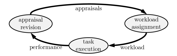
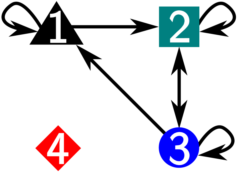
In this paper, we focus on a quantitative model describing the process by which individuals in a team evaluate one another while concurrently assigning work to each of the team members, in order to maximize the collective team performance (see Figure 1). More specifically, we assume each team member is endowed with a skill level (a-priori unknown), and that the team needs to divide a complex task among its members. We let each team member build their own local appraisal of neighboring team members’ based on the performance exhibited on previous tasks. Upcoming tasks are then distributed according to the current appraisal estimates. Finally, the performance of each member is newly observed by neighboring members, who, in turn, update their appraisal. Any model satisfying these assumptions is composed of two building blocks: i) an appraisal component modeling how team members update their appraisals (left block in Figure 1), and ii) a work assignment component describing how the task is divided within the team (right block in Figure 1).

Refer to caption — Figure 1: Architectural overview on the assign and appraise model studied in this manuscript. Given a complex task to complete, team members get assigned and execute an initial workload (right and bottom blocks). Each team member revises their appraisal of neighboring members based on each neighbor’s individual performance (left), which in turn is used to reassign the workload. The objective is for the team to learn who has what skill, so as to assign tasks in a way that maximizes the collective team performance.

We model the appraisal process i) through the lens of transactive memory systems, a conceptual model introduced by Wegner [23], which assumes that a team is capable of developing collective knowledge regarding who has what information and capabilities. Our choice of dynamics describing the evolution of the interpersonal appraisals is inspired from replicator dynamics, whereby each team member $i$ updates their appraisal of a neighboring member $j$ proportionally to the difference between member $j$ performance and the (appraisal-weighted) average performance of the team.

We model the work assignment process ii) as a compartmental system [14], and utilize two natural dynamics to describe how the task is divided based on the current appraisals. These dynamics correspond to utilizing different centrality measures to subdivide a complex task. It is crucial to observe that the coupling between the appraisal revision and the work assignment process results in a coevolutionary network problem.

This paper follows a trend initiated recently, whereby many traditionally qualitative fields such as social psychology and organizational sciences are developing quantitative models. In this regard, our aim is to quantify the development of transactive memory within a team and study what conditions cause a team to fail or succeed at allocating a task optimally among members. To do so, we leverage control theoretical tools as well as ideas from evolutionary game theory, and notions from graph theory.

I-B Contributions

Our main contributions are as follows.

(i)

We formulate a quantitative model to capture the coevolution of the workload division and appraisal network, where the optimal workload assignment maximizing the collective team performance is an equilibrium of the model. While we let the appraisal network evolve according to a replicator-like dynamics, we consider two different mechanisms for workload division and show well-posedness of the model.
(ii)

Regardless of the mechanism used for workload division, we derive conserved quantities associated to the cycles of the appraisal network. Leveraging this result, for a team of $n$ individuals, we significantly reduce the dimension of the system from $n^{2}+n$ to a $2n$ dimensional submanifold.
(iii)

We provide rigorous positive and negative results that characterize the asymptotic behavior for either of the workload division mechanisms. When adopting the first workload division mechanism, we show that under a mild assumption, strongly connected teams are always able to learn each member’s correct skill level, and thus determine the optimal workload division. In the second model variation, strong connectivity is insufficient to guarantee that the team learns the optimal workload, but more specific assumptions allow the team to converge to the optimal workload.
(iv)

Finally, we enrich our analysis by means of numerical experiments that provide further insight into the limiting behavior.

I-C Related works

Quantitative models of transactive memory systems

Wegner’s transactive memory systems (TMS) model [23] describes how cognitive states affect the collective performance of a team performing complex tasks. This widely established model captures both learning on the individual and collective level, as well as the evolution of the interaction between individuals within a team.

There are very few quantitative models attempting to describe TMS and most of these models rely on numerical analysis to study the evolution of team knowledge [10], or what events are disruptive to learning and productivity in groups [1]. However, numerical analysis alone has natural limitations, whereas a mathematical perspective to TMS can establish the emergence of learning behaviors for entire classes of models. Moreover, while our proposed model is agent-based with collective knowledge represented as a weighted digraph, [10, 1] are not agent-based models and use a scalar value to encode the team’s collective knowledge.

The collective learning model introduced by Mei et al. [16] was the first to quantify TMS with appraisal networks and provide convergence analysis. In particular, for the assign/appraise model in [16], the appraisal update protocol is akin to one originally introduced in [7] and assumes each team member only updates their own appraisal based on performance comparisons. Additionally, the workload assignment is a centralized process determined by the eigenvector centrality of the network [3]. Our model significantly differs from [16] in that team members update their own and neighboring team members’ appraisals. Additionally, the workload assignment is a distributed and dynamic process.

Distributed optimization

Our model has direct ties with the field of distributed optimization. Under suitable conditions discussed later, in fact, the team will be able to learn each other’s skill levels, and thus agree on a work assignment maximizing the collective performance in a distributed fashion. Additionally, any change in the problem dimension, due to the addition or subtraction of agents, only requires local adaptions. In light of this observation, one could reinterpret the assign and appraisal model studied here as a distributed optimization algorithm, where the objective is that of maximizing the team performance through local communication. In comparison to our work, existing distributed optimization algorithms often require more complex dynamics. For example, [17] requires that the optimal solution estimates are projected back into the constrained set, while Newton-like methods [24] require higher order information.

Perhaps closest to this perspective on our problem is the work of Barreiro-Gomez et al. [2], where evolutionary game theory is used to design distributed optimization algorithms. Nevertheless, we observe that the objective we pursue here is that of quantifying if and to what extent team members learn how to share a task optimally. In this respect, the dynamics we consider do not arise as the result of a design choice (as it is in [2]), but they are rather defining the problem itself.

Adaptive coevolutionary networks

Our model is an example of appraisal network coevolving with a resource allocation process. Research regarding adaptive networks has gained traction in recent decades, appearing in biological systems and game theoretical applications [11]. Wang et al. [22], for example, review coupled disease-behavior dynamics, while Ogura et al. [19] propose an epidemic model where awareness causes individuals to distance themselves from infected neighbors. Finally, we note that coevolutionary game theory considers dynamics on the population strategies and dynamics of the environment, where the payoff matrix evolves with the environment state [26, 8].

I-D Paper organization

Section II contains the problem framework, model definition, the model’s well-posedness, and equilibrium corresponding to the optimal workload. Section III contains the properties of the appraisal dynamics and reduced order dynamics. Section IV and V present the convergence results for the model with both workload division mechanisms. Section VI contains numerical studies illustrating the various cases of asymptotic behavior.

I-E Notation

Let $\mathbbold{1}_{n}$ ( $\mathbbold{0}_{n}$ resp.) denote the $n$ -dimensional column vector with all ones (zero resp.). Let $I_{n}$ represent the $n\times n$ identity matrix. For a matrix or vector $B\in^{n\times m}$ , let $B\geq 0$ and $B>0$ denote component-wise inequalities. Given $x=[x_{1},\dots,x_{n}]^{\top}\in^{n}$ , let $\operatorname{diag}(x)$ denote the $n\times n$ diagonal matrix such that the $i$ th entry on the diagonal equals $x_{i}$ . Let $\odot$ ( $\oslash$ resp.) denote Hadamard entrywise multiplication (division resp.) between two matrices of the same dimensions. For $x,y\in^{n}$ and $B\in^{n\times n}$ , we shall use the property

xy^{\top}\odot B=\operatorname{diag}(x)B\operatorname{diag}(y).

(1)

Define the $n$ -dimensional simplex as $\Delta_{n}=\{x\in^{n}\;|\;\mathbbold{1}_{n}^{\top}x=1,x\geq 0\}$ and the relative interior of the simplex as $\mathrm{int}(\Delta_{n})=\{x\in\mathbb{R}^{n}\;|\;\mathbbold{1}_{n}^{\top}x=1,x>0\}$ .

A nonnegative matrix $B\geq 0$ is row-stochastic if $B\mathbbold{1}_{n}=\mathbbold{1}_{n}$ . For a nonnegative matrix $B$ , $G(B)$ is the weighted digraph associated to $B$ , with node set $\{1,\dots,n\}$ and directed edge $(i,j)$ from node $i$ to $j$ if and only if $b_{ij}>0$ . A nonnegative matrix $B$ is irreducible if its associated digraph is strongly connected. The Laplacian matrix of a nonnegative matrix $B$ is defined as $L(B)=\operatorname{diag}(B\mathbbold{1}_{n})-B$ . For $B$ irreducible and row-stochastic, $v_{\textup{left}}(B)$ denotes the left dominant eigenvector of $B$ , i.e., the entry-wise positive left eigenvector normalized to have unit sum and associated with the dominant eigenvalue of $B$ [6, Perron Frobenius theorem].

II Problem Framework and ASAP Model

In this section, we first propose the Assignment and Appraisal (ASAP) model and establish that it is well-posed for finite time. The proposed ASAP model can be considered a socio-inspired, distributed, and online algorithm for optimal resource allocation problems. Our model captures two fundamental processes within teams: workload distribution and transactive memory. We consider two distributed, dynamic models for the workload division: a compartmental system model and a linear model that uses average-appraisal as the input for adjusting workload. The transactive memory is quantified by the appraisal network and reflects individualized peer evaluation in the team. The development of the transactive memory system allows the team to estimate the work assignment that maximizes the collective team performance.

II-A Workload assignment, performance observation, and appraisal network

Workload assignment

We consider a team of $n$ individuals performing a sequence of tasks. Let $\bm{w}=[w_{1},\dots,w_{n}]^{\top}\in\mathrm{int}(\Delta_{n})$ denote the vector of workload assignments for a given task, where $w_{i}$ is the work assignment of individual $i$ .

Individual performance

Let $p(\bm{w}):\mathrm{int}(\Delta_{n})\rightarrow\mathbb{R}_{{>0}}^{n}$ represent the vector of individual performances that change as a function of the work assignment, where $p(\bm{w})=[p_{1}(w_{1}),\dots,p_{n}(w_{n})]^{\top}\in$ and $p_{i}(w_{i})$ is the performance of individual $i$ . In general, individuals will perform better if they have less workload; we formalize this notion with the following two assumptions.

Assumption 1.

(Smooth and strictly decreasing performance functions) Assume function $p_{i}:(0,1]\rightarrow[0,\infty)$ is $C^{1}$ , strictly decreasing, convex, integrable, and $\lim_{x\to 0^{+}}p_{i}(x)=+\infty$ .

Assumption 2.

(Power law performance functions) Assume function $p_{i}:(0,1]\rightarrow[0,\infty)$ is of the form $p_{i}(x)=s_{i}x^{-\gamma}$ where $s_{i}>0$ and $\gamma\in(0,1)$ .

The first assumption is quite general and can be further weakened at the cost of additional notation. The second assumption is more restrictive than Assumption 1, but is well-motivated by the power law for individual learning [18]. Note that functions obeying Assumption 2 also satisfy Assumption 1.

Appraisal network

Let $A=\{a_{ij}\}_{i,j\in\{1,\dots,n\}}$ denote the $n\times n$ nonnegative, row-stochastic appraisal matrix, where $a_{ij}$ is individual $i$ ’s appraisal of individual $j$ . The appraisal matrix represents the team’s network structure and transactive memory system.

II-B Model description and problem statement

In this work, we design a model where the workload assignment coevolves with the appraisals: the workload assignment changes as a function of the appraisals and the appraisals update based on perceived performance disparities for the assigned workload. Suppose at each time $t$ , the team has a workload assignment $\bm{w}(t)$ , individual performances $p(\bm{w}(t))$ , and appraisal matrix $A(t)$ . Since we are studying teams, it is reasonable to assume the appraisal network is strongly connected and each individual appraises themself. This translates to an irreducible initial appraisal matrix $A(0)$ with strictly positive self-appraisals $a_{ii}(0)>0$ for all $i\in\{1,\dots,n\}$ . All members also start with strictly positive workload $\bm{w}(0)\in\mathrm{int}(\Delta_{n})$ . For shorthand throughout the rest of the paper, we use $A_{0}=A(0)$ and $\bm{w}_{0}=\bm{w}(0)$ .

Before introducing the model, first we define the work flow function $F=[F_{1}(A,\bm{w}),\dots,F_{n}(A,\bm{w})]^{\top}$ , where $F_{i}:[0,1]^{n\times n}\times\Delta_{n}\rightarrow\Delta_{n}$ describes how individual $i$ adjusts their own work assignment. Then our coevolving assignment and appraisal process is quantified by the following dynamical system.

Definition 3 (ASAP (assignment and appraisal) model).

Consider $n$ performance functions $p_{i}$ satisfying Assumption 1 or 2. The coevolution of the appraisal network $A(t)$ and workload assignment $\bm{w}(t)$ obey the following coupled dynamics,

\begin{split}\dot{a}_{ij}&=a_{ij}\Big{(}p_{j}(w_{j})-\sum_{k=1}^{n}a_{ik}p_{k}(w_{k})\Big{)},\\ \dot{w}_{i}&=F_{i}(A,\bm{w}),\end{split}

(2)

which reads in matrix form

\begin{split}\dot{A}&=A\odot\Big{(}\mathbbold{1}_{n}p(\bm{w})^{\top}-Ap(\bm{w})\mathbbold{1}_{n}^{\top}\Big{)},\\ \dot{\bm{w}}&=F(A,\bm{w}).\end{split}

(3)

The work flow function $F$ obeys one of the following work flow models:

	Donor-controlled:	$\displaystyle F_{i}(A,\bm{w})=-w_{i}+\sum_{k=1}^{n}a_{ki}w_{k},$		(4)
	Average-appraisal:	$\displaystyle F_{i}(A,\bm{w})=-w_{i}+\frac{1}{n}\sum_{k=1}^{n}a_{ki}.$		(5)

The matrix forms of the donor-controlled (4) and average-appraisal (5) work flows are $F(A,\bm{w})=-\bm{w}+A^{\top}\bm{w}$ and $F(A,\bm{w})=-\bm{w}+\frac{1}{n}A^{\top}\mathbbold{1}_{n}$ , respectively.

The appraisal weights of the ASAP model (2) update based on performance feedback between neighboring individuals. For neighboring team members $i$ and $j$ , $i$ will increase their appraisal of $j$ if $j$ ’s performance is larger than the weighted average performance observed by $i$ , i.e. $p_{j}(w_{j})>\sum_{k=1}^{n}a_{ik}p_{k}(w_{k})$ . Individual $i$ also updates their self-appraisal with the same mechanism. The irreducibility and strictly positive self-appraisal assumptions on the appraisal network means that every individual’s performance is evaluated by themself and at least one other individual within the team.

The donor-controlled work flow (4) models a team where individuals exchange portions of their workload assignment with their neighbors, and the amount of work exchanged depends on their current work assignments and the appraisal values. The work individual $j$ gives to individual $i$ has flow rate $a_{ji}$ and is proportional to $w_{j}$ . The average-appraisal work flow (5) assumes that each individual collects feedback from neighboring team members through appraisal evaluations. Each individual uses this feedback to calculate their average-appraisal $\frac{1}{n}\sum_{k=1}^{n}a_{ki}$ , which is then used to adjust their own workload assignment. The average-appraisal is equivalent to the degree centrality of the appraisal network. Note that while the donor-controlled work flow is decentralized and distributed, the average-appraisal work flow is only distributed since it requires individuals to know the total number of team members.

In the following lemma, we show that the ASAP model is well-posed and the appraisal network maintains the same network topology for finite time.

Lemma 4 (Finite-time properties for the ASAP model).

Consider the ASAP model 2 with donor controlled (4) or average appraisal (5) work flow. Assume $A_{0}$ is row-stochastic, irreducible, with strictly positive diagonal and $\bm{w}_{0}\in\mathrm{int}(\Delta_{n})$ . Then for any finite $\Delta t>0$ , the following statements hold:

(i)

$\bm{w}(t)\in\mathrm{int}(\Delta_{n})$ for $t\in[0,\Delta t]$ ;
(ii)

$A(t)$ remains row-stochastic with the same zero/positive pattern for $t\in[0,\Delta t]$ .

Proof.

Before proving statement (i), we give some properties of the appraisal dynamics. If $a_{ij}(t)=0$ , then $\dot{a}_{ij}(t)=0$ , which implies $a_{ij}(t)\geq 0$ . By using the Hadamard product property (1), the matrix form of the appraisal dynamics can also be written as $\dot{A}=A\operatorname{diag}(p(\bm{w}))-\operatorname{diag}(Ap(\bm{w}))A$ . Then for $A_{0}\mathbbold{1}_{n}=\mathbbold{1}_{n}$ , $\dot{A}\mathbbold{1}_{n}=\mathbbold{0}_{n}$ , so $A(t)$ remains row-stochastic for $t\geq 0$ .

Next, we use $A(t)$ row-stochastic to prove $w(t)\in\mathrm{int}(\Delta_{n})$ for donor-controlled work flow and $t\in[0,\Delta t]$ . Left multiplying the $\bm{w}(t)$ dynamics by $\mathbbold{1}_{n}^{\top}$ , we have $\mathbbold{1}_{n}^{\top}\dot{\bm{w}}=\mathbbold{1}_{n}^{\top}(-\bm{w}+A^{\top}\bm{w})=\mathbbold{0}_{n}$ . Next, let $w_{i}(t)=\min_{k}\{w_{k}(t)\}$ . For $\bm{w}_{0}\in\mathrm{int}(\Delta_{n})$ , $w_{i}(t)=\min_{k}\{w_{k}(t)\}=0$ , and $A(t)\geq 0$ , then $\dot{w}_{i}(t)=\sum_{k=1}^{n}a_{ki}(t)w_{k}(t)\geq 0$ . Therefore $\bm{w}(t)\in\Delta_{n}$ . Lastly, we apply the Grönwall-Bellman Comparison Lemma to also show that $\bm{w}(t)$ lives in the relative interior of the simplex. For $w_{i}(0)>0$ and $\dot{w}_{i}(t)=-w_{i}(t)+\sum_{k=1}^{n}a_{ki}(t)w_{k}(t)\geq-w_{i}(t)$ , then $w_{i}(t)\geq w_{i}(0)e^{-t}>0$ for $t\in[0,\Delta t]$ . Therefore, if $\bm{w}_{0}\in\mathrm{int}(\Delta_{n})$ , then $\bm{w}(t)\in\mathrm{int}(\Delta_{n})$ for $t\in[0,\Delta t]$ .

The proof for statement (i) can be extended to the average-appraisal work flow (5) following the same process, since $\dot{w}_{i}(t)=-w_{i}(t)+\frac{1}{n}\sum_{k=1}^{n}a_{ki}(t)\geq-w_{i}(t)$ .

For statement (ii), to prove that $A(t)$ maintains the same zero/positive pattern for $t\in[0,\Delta t]$ , consider any $i,j$ such that $a_{ij}(0)>0$ . Since $\bm{w}(t)\in\mathrm{int}(\Delta_{n})$ , then $p(\bm{w}(t))>0$ by the performance function assumptions and $p_{j}(w_{j})-\sum_{k=1}^{n}a_{ik}p_{k}(w_{k})$ is finite for any $i,j$ and $t\in[0,\Delta t]$ . Let $p_{\max}(\bm{w}(t))=\max_{k\in\{1,\dots,n\}}\{p_{k}(w_{k})\}$ . Then the convex combination of individual performances is upper bounded by $\sum_{k=1}^{n}a_{ik}p_{k}(w_{k})\leq p_{\max}(\bm{w}(t))$ . Now we can write the following lower bound for the time derivative of $a_{ij}(t)$ ,

	$\displaystyle\dot{a}_{ij}(t)$	$\displaystyle\geq a_{ij}(t)\big{(}p_{j}(w_{j}(t))-\sum\nolimits_{k=1}^{n}a_{ik}(t)p_{k}(w_{k}(t))\big{)}$
		$\displaystyle\geq-a_{ij}(t)p_{\max}(\bm{w}(t)).$

Using the Grönwall-Bellman Comparison Lemma again, for $t\in[0,\Delta t]$ , then

\displaystyle a_{ij}(t)

\displaystyle\geq a_{ij}(0)\exp\bigg{(}-\int_{0}^{t}p_{\max}(\bm{w}(\tau))d\tau\bigg{)}>0.

Therefore, $A(t)$ remains row-stochastic and maintains the same zero/positive pattern as $A_{0}$ for finite time. ∎

II-C Team performance and optimal workload as model equilibria

We are interested in the collective team performance and while no single collective team performance function is widely accepted in the social sciences, we consider three such functions. Under minor technical assumptions, the optimal workload for all three is characterized by equal performance levels by the individuals and is an equilibrium point of the ASAP model. If $p_{i}(w_{i})$ represents the marginal utility of individual $i$ , then the collective team performance can be measured by the total utility,

\mathcal{H}_{\textup{tot}}(\bm{w})=\sum_{i=1}^{n}\int_{0}^{w_{i}}p_{i}(x)dx.

The team performance can alternatively be measured by the “weakest link” or minimum performer,

\mathcal{H}_{\textup{min}}(\bm{w})=\min_{i\in\{1,\dots,n\}}\{p_{i}(w_{i})\}.

Another metric often used is the weighted average individual performance:

\mathcal{H}_{\textup{avg}}(\bm{w})=\sum_{i=1}^{n}w_{i}p_{i}(w_{i}).

The next theorem clarifies when the workload maximizing either $\mathcal{H}_{\textup{tot}}$ , $\mathcal{H}_{\textup{min}}$ , or $\mathcal{H}_{\textup{avg}}$ is an equilibrium of the ASAP model.

Theorem 5 (Optimal performance as equilibria of dynamics).

Consider performance functions $p_{i}$ satisfying Assumption 1 for all $i\in\{1,\dots,n\}$ . Then

(i)

there exists a unique pair $(p^{*},\bm{w}^{\mathrm{opt}})$ such that $p^{*}>0$ , $\bm{w}^{\mathrm{opt}}\in\mathrm{int}(\Delta_{n})$ , and $p(\bm{w}^{\mathrm{opt}})=p^{*}\mathbbold{1}_{n}$ .

Additionally, let $\mathcal{H}$ denote $\mathcal{H}_{\textup{tot}}$ , $\mathcal{H}_{\textup{min}}$ , or $\mathcal{H}_{\textup{avg}}$ . Let Assumption 2 hold when $\mathcal{H}=\mathcal{H}_{\textup{avg}}$ . Then

(ii)

$\bm{w}^{\mathrm{opt}}$ is the unique solution to

$\bm{w}^{\mathrm{opt}}=\operatorname*{arg\,max}_{\bm{w}\in\Delta_{n}}\{\mathcal{H}(\bm{w})\}.$

Finally, consider the ASAP model (2) with donor-controlled work flow (4) and let $A_{0}$ be row-stochastic, irreducible, with strictly positive diagonal and $\bm{w}_{0}\in\mathrm{int}(\Delta_{n})$ . Then

(iii)

there exists at least one matrix $A^{*}$ with the same zero/positive pattern as $A_{0}$ that satisfies $\bm{w}^{\mathrm{opt}}=v_{\textup{left}}(A^{*})$ ; and
(iv)

every pair $(A^{*},\bm{w}^{\mathrm{opt}})$ , such that $A^{*}$ has the same zero/positive pattern as $A_{0}$ and $\bm{w}^{\mathrm{opt}}=v_{\textup{left}}(A^{*})$ , is an equilibrium.

For average-appraisal work flow (5), statements (iii)-(iv) may not hold for $\bm{w}^{\mathrm{opt}}=\frac{1}{n}(A^{*})^{\top}\mathbbold{1}_{n}$ , since there may not exist an $A^{*}$ with the same zero/positive pattern as $A_{0}$ . Section V elaborates on these results.

Proof.

Regarding statement (i), recall that $p_{i}$ is $C^{1}$ and strictly decreasing by Assumption 1 or 2. Now we show that given our assumptions, there exists $\bm{w}^{\mathrm{opt}}\in\mathrm{int}(\Delta_{n})$ such that $p(\bm{w}^{\mathrm{opt}})=p^{*}\mathbbold{1}_{n}$ holds. Let $p_{i}^{-1}$ denote the inverse of $p_{i}$ and let $\circ$ denote the composition of functions where $f(g(x))=(f\circ g)(x)$ . Given $p_{1}(w_{1})=p_{i}(w_{i})$ , then $w_{i}=(p^{-1}_{i}\circ p_{1})(w_{1})$ for all $i\neq 1$ . Then taking into account $\bm{w}^{\mathrm{opt}}\in\mathrm{int}(\Delta_{n})$ ,

w_{1}+\sum\nolimits_{i=1}^{n}(p^{-1}_{i}\circ p_{1})(w_{1})=1.

$p_{i}$ strictly decreasing implies $p_{i}^{-1}$ ( $p_{i}^{-1}\circ p_{1}$ resp.) is strictly decreasing (strictly increasing resp.). Therefore the left hand side of the above equation is strictly increasing, so there is a unique $w^{\mathrm{opt}}_{1}\in(0,1)$ solving the equation. Therefore there is a unique $(p^{*},\bm{w}^{\mathrm{opt}})$ that satisfies $p(\bm{w}^{\mathrm{opt}})=p^{*}\mathbbold{1}_{n}$ , where $p^{*}=p_{1}(w^{\mathrm{opt}}_{1})>0$ .

Regarding statement (ii), $p_{i}$ is strictly decreasing, $C^{1}$ , and convex by Assumption 1-2. Then $\mathcal{H}_{\textup{tot}}$ , $\mathcal{H}_{\textup{min}}$ , and $\mathcal{H}_{\textup{avg}}$ are all strictly concave. Since we are maximizing over a compact set, and $\mathcal{H}(\bm{w})$ is finite for $\bm{w}\in\Delta_{n}$ , there exists a unique optimal solution $\bm{w}^{\mathrm{opt}}\in\Delta_{n}$ . Next we show that $\bm{w}^{\mathrm{opt}}$ must satisfy $p(\bm{w}^{\mathrm{opt}})=p^{*}\mathbbold{1}_{n}$ where $p^{*}>0$ for each collective team performance measure and $\bm{w}^{\mathrm{opt}}\in\mathrm{int}(\Delta_{n})$ .

First, consider $\mathcal{H}=\mathcal{H}_{\textup{tot}}$ . Let $\bm{\mu}\in^{n}$ and $\lambda\in$ . Then the KKT conditions are given by: $p(\bm{w}^{\mathrm{opt}})+\bm{\mu}-\lambda\mathbbold{1}_{n}=\mathbbold{0}_{n}$ , $\bm{\mu}\odot\bm{w}^{\mathrm{opt}}=\mathbbold{0}_{n}$ , and $\bm{\mu}\succeq\mathbbold{0}_{n}$ . If $\lambda\to\infty$ , then $\bm{w}^{\mathrm{opt}}=\mathbbold{0}_{n}$ for the first KKT condition to hold, but we require $\bm{w}^{\mathrm{opt}}\in\Delta_{n}$ . Similarly, $w^{\mathrm{opt}}_{i}=0$ for any $i$ would satisfy the second KKT condition, but violate the first KKT condition. As a result, $\lambda<\infty$ and $\bm{\mu}=\mathbbold{0}_{n}$ . This implies that $p_{i}(w^{\mathrm{opt}}_{i})=\lambda$ for all $i$ . Therefore $\bm{w}^{\mathrm{opt}}\in\mathrm{int}(\Delta_{n})$ and there exists $p^{*}=\lambda\in(0,\infty)$ such that $p(\bm{w}^{\mathrm{opt}})=p^{*}\mathbbold{1}_{n}$ .

Second, consider $\mathcal{H}=\mathcal{H}_{\textup{min}}$ . Define the set $\operatorname*{arg\,min}(p(\bm{w}))=\{i\in\{1,\dots,n\}\;|\;p_{i}(w_{i})=\min_{k}\{p_{k}(w_{k})\}\}$ and let $|\operatorname*{arg\,min}(p(\bm{w}))|$ denote the number of elements in $\operatorname*{arg\,min}(p(\bm{w}))$ . We prove the claim by contradiction. Assume $\bm{w}^{\mathrm{opt}}$ is the optimal solution such that there exists at least one $j\neq i$ such that $p_{i}(w^{\mathrm{opt}}_{i})<p_{j}(w^{\mathrm{opt}}_{j})$ for $i\in\operatorname*{arg\,min}(p(\bm{w}))$ . Then there exists a sufficiently small $\epsilon>0$ and $\bm{w}^{*}\in\mathrm{int}(\Delta_{n})$ such that $\mathcal{H}_{\textup{min}}(\bm{w}^{\mathrm{opt}})<\mathcal{H}_{\textup{min}}(\bm{w}^{*})$ , where $w^{*}_{i}=w^{\mathrm{opt}}_{i}-\epsilon$ and $w^{*}_{j}=w^{\mathrm{opt}}_{j}+\epsilon|\operatorname*{arg\,min}(p(\bm{w}))|$ . This contradicts the fact that $\bm{w}^{\mathrm{opt}}$ is the optimal solution. Additionally, we can prove that $\bm{w}^{\mathrm{opt}}\in\mathrm{int}(\Delta_{n})$ by assuming there exists at least one $i$ such that $w_{i}=0$ and following the same proof by contradiction process. Therefore $\bm{w}^{\mathrm{opt}}\in\mathrm{int}(\Delta_{n})$ and $p(\bm{w}^{\mathrm{opt}})=p^{*}\mathbbold{1}_{n}$ .

Third, consider $\mathcal{H}=\mathcal{H}_{\textup{avg}}$ . Let $\bm{\mu}\in^{n}$ and $\lambda\in$ . Then the KKT conditions are given by: $(1-\gamma)p(\bm{w}^{*})+\bm{\mu}-\lambda\mathbbold{1}_{n}=\mathbbold{0}_{n}$ , $\bm{\mu}\odot\bm{w}^{*}=\mathbbold{0}_{n}$ , and $\bm{\mu}\succeq\mathbbold{0}_{n}$ . The rest of the proof follows from the same argument as used for $\mathcal{H}=\mathcal{H}_{\textup{tot}}$ .

Regarding statements (iii) and (iv), let $a_{d}=[a_{11},\dots,a_{nn}]^{\top}\in[0,1]^{n}$ and $A(a_{d},A_{0})=\operatorname{diag}(a_{d})+(I_{n}-\operatorname{diag}(a_{d}))A_{0}$ . We prove that there exists some $a_{d}^{*}>0$ such that $\bm{w}^{\mathrm{opt}}=v_{\textup{left}}\big{(}A^{*}(a_{d}^{*},A_{0})\big{)}$ . From the assumptions on $A_{0}$ , then there exists $\bar{\bm{w}}=v_{\textup{left}}(A_{0})$ such that $\sigma\bar{\bm{w}}=(I_{n}-\operatorname{diag}(a_{d}^{*}))\bm{w}^{\mathrm{opt}}$ for $\sigma\in$ . Then solving for $a_{d}^{*}$ , we have $a_{d}^{*}=\mathbbold{1}_{n}-\sigma(\bar{\bm{w}}\oslash\bm{w}^{\mathrm{opt}})$ . Next, we choose $\sigma=\epsilon/\max_{i}\{\bar{w}_{i}/w_{i}\}$ for $\epsilon\in(0,1)$ , which gives the following bounds on $a_{ii}$ for all $i$ ,

a_{ii}\in[1-\epsilon,1-\epsilon\min_{i}\{\bar{w}_{i}/w_{i}\}(\max_{i}\{\bar{w}_{i}/w_{i}\})^{-1}]\subseteq(0,1).

With $a_{d}^{*}>\mathbbold{0}_{n}$ , then $A^{*}(a_{d}^{*},A_{0})$ has the same zero/positive pattern as $A(0)$ . This shows that, given $\bm{w}^{\mathrm{opt}}$ , there always exists a matrix $A^{*}$ with left dominant eigenvector $\bm{w}^{\mathrm{opt}}$ and with the same pattern as $A(0)$ .

Next, we prove that any such pair $(A^{*},\bm{w}^{\mathrm{opt}})$ is an equilibrium. Our assumptions on $A^{*}$ and the Perron-Frobenius theorem together imply that the $\mathrm{rank}(I_{n}-(A^{*})^{\top})=n-1$ . For the ASAP model (2) with donor-controlled work flow (4), the equilibrium conditions on the self-appraisal states and work assignment read:

	$\displaystyle\mathbbold{0}_{n}$	$\displaystyle=\operatorname{diag}\big{(}a_{d}(A^{})\big{)}(I_{n}-A^{})p(\bm{w}^{*}),$		(6)
	$\displaystyle\mathbbold{0}_{n}$	$\displaystyle=(A^{}-I_{n})^{\top}\bm{w}^{}.$		(7)

Equation (6) is satisfied because we know from statement (ii) that $p(\bm{w}^{\mathrm{opt}})=p^{*}\mathbbold{1}_{n}$ . Equation (7) is satisfied because we know $v_{\textup{left}}(A^{*})=\bm{w}^{\mathrm{opt}}$ . This concludes the proof of statements (iii) and (iv). ∎

The equilibria described in the above lemma also resemble an evolutionarily stable set [12], which is defined as the set of strategies with the same payoff. Our proof illustrates that at least one $A^{*}$ always exists, but in general, there are multiple $A^{*}$ matrices that satisfy a particular zero/positive irreducible matrix pattern with $\bm{w}^{\mathrm{opt}}=v_{\textup{left}}(A^{*})$ with the same collective team performance. We will later show that, under mild conditions, this optimal solution is an equilibrium of our dynamics with various attractivity properties (see Section IV and V).

III Properties of Appraisal Dynamics: Conserved Quantities and Reduced Order Dynamics

In this section, we show that every cycle in the appraisal network is associated to a conserved quantity. Leveraging these conserved quantities, we reduce the appraisal dynamics to an $n-1$ dimensional submanifold. Before doing so, we introduce the notion of cycles, cycle path vectors, the cycle set, and the cycle space. For a given initial appraisal matrix $A_{0}$ with strictly positive diagonal, let $m$ denote the total number of strictly positive interpersonal appraisals in the edge set $\mathcal{E}(A_{0})$ . Recall that if $a_{ij}(0)=0$ for any $i,j$ , then $\dot{a}_{ij}=0$ , which implies $a_{ij}(t)=0$ for all $t\geq 0$ . Therefore we can consider the total number of appraisal states to be the number of edges in $A_{0}$ , which gives a total of $n+m$ appraisal states.

Definition 6 (Cycles, cycle path vectors, and cycle set).

Consider the digraph $G(A)$ associated to matrix $A\in\mathbb{R}_{\geq 0}^{n\times n}$ .

A cycle is an ordered sequence of nodes $r=\{r_{1},\dots,r_{k},r_{1}\}$ with no node appearing more than once, that starts and ends at the same node, has at least two distinct nodes, and each sequential pair of nodes in the cycle denotes an edge $(r_{i},r_{i+1})\in\mathcal{E}(A)$ . We do not consider self-loops, i.e. self-appraisal edges, to be part of any cycles.

Let $C_{r}\in\{0,1\}^{m}$ denote the cycle path vector associated to cycle $r$ . Let each off-diagonal edge of the appraisal matrix $(i,j)\in\mathcal{E}(A)$ be assigned to a number in the ordered set $\{1,\dots,m\}$ . For every edge $e\in\{1,\dots,m\}$ , the $e$ th component of $C_{r}$ is defined as

\displaystyle(C_{r})_{e}=\begin{cases}+1,&\;\text{if edge }e\text{ is positively traversed by }C_{r},\\ 0,&\;\text{otherwise}.\end{cases}

Let $\Phi(A)$ denote the cycle set, i.e. the set of all cycles, in digraph $G(A)$ .

To refer to a particular cycle, we will use the cycle’s associated cycle path vector, which then allows us to define the cycle space.

Definition 7 (Cycle space).

A cycle space is a subspace of ^m spanned by cycle path vectors. By [4, pg. 29, Theorem 9], the cycle space of a strongly connected digraph $G(A)$ is spanned by a basis of $\mu=m-n+1$ cycle path vectors.

Let $C_{B}\in\{0,1\}^{m\times\mu}$ denote a matrix where the columns are a basis of the cycle space.

The following theorem (i) rigorously defines the conserved quantities associated to cycles in the appraisal network; (ii) shows that the appraisal states can be reduced from dimension $n+m$ to $n-1$ using the conserved quantities; and (iii) uses both the previous properties to introduce reduced order dynamics that have a one-to-one correspondence with the appraisal trajectories.

Theorem 8 (Conserved cycle constants give reduced order dynamics).

Consider the ASAP model (3) with donor-controlled (4) or average-appraisal (5) work flow. Given initial conditions $A_{0}$ row-stochastic, irreducible, with strictly positive diagonal and $\bm{w}_{0}\in\mathrm{int}(\Delta_{n})$ , let $(A(t),\bm{w}(t))$ be the resulting trajectory. Then

(i)

for any cycle $r$ , the quantity

$c_{r}=\prod_{(i,j)\in r}\frac{a_{ii}(t)}{a_{ij}(t)},$ (8)

is constant; we refer to $c_{r}\in(0,\infty)$ as the cycle constant associated to cycle $r\in\Phi(A_{0})$ ;
(ii)

the appraisal matrix $A(t)$ takes value in a submanifold of dimension $n-1$ ;

(iii)

given a solution $(\bm{v}(t),\bar{\bm{w}}(t))\in_{>0}^{n}\times\mathrm{int}(\Delta_{n})$ with initial condition $(\bm{v}_{0},\bar{\bm{w}}_{0})=(\mathbbold{1}_{n},\bm{w}_{0})$ of the dynamics

\begin{split}\dot{\bm{v}}&=\operatorname{diag}\big{(}p(\bar{\bm{w}})-\bar{\bm{w}}^{\top}\mathcal{A}(\bm{v})p(\bar{\bm{w}})\mathbbold{1}_{n}\big{)}\bm{v},\\ \dot{\bar{\bm{w}}}&=F(\mathcal{A}(\bm{v}),\bar{\bm{w}}),\end{split}

(9)

where $\mathcal{A}:^{n}\to^{n\times{n}}$ is defined by

\begin{split}\mathcal{A}(\bm{v})&=\operatorname{diag}(A_{0}\bm{v})^{-1}A_{0}\operatorname{diag}(\bm{v}),\end{split}

(10)

then $A(t)=\mathcal{A}(\bm{v}(t))$ and $\bm{w}(t)=\bar{\bm{w}}(t)$ ;

(iv)

for every equilibrium $(\bm{v}^{*},\bm{w}^{\mathrm{opt}})$ of (9), $(A^{*},\bm{w}^{\mathrm{opt}})$ is an equilibrium of (3) with $A^{*}=\mathcal{A}(\bm{v}^{*})$ ;
(v)

if additionally $A_{0}>0$ , then the positive matrix $A(t)\oslash A_{0}$ is rank 1 for all time $t$ .

Proof.

Regarding statement (i), we show that $c_{r}$ is constant for any $r\in\Phi(A_{0})$ by taking the natural logarithm of both sides of (8) and showing that the derivative vanishes. By Lemma 4, $\ln(c_{r})$ is well-defined since $a_{ii}(t),a_{ij}(t)>0$ for any $a_{ij}\in r$ and finite time $t<\infty$ .

\diff{}{t}\ln(c_{r})=\sum_{(i,j)\in r}\Big{(}\frac{\dot{a}_{ii}}{a_{ii}}-\frac{\dot{a}_{ij}}{a_{ij}}\Big{)}\\ =\sum_{(i,j)\in r}\Big{(}\big{(}p_{i}(w_{i})-\bar{p}_{i}(\bm{w})\big{)}-\big{(}p_{j}(w_{j})-\bar{p}_{i}(\bm{w})\big{)}\Big{)}=0.

Therefore, $c_{r}$ is constant for all $r\in\Phi(A_{0})$ .

Regarding statement (ii), first, we will introduce a change of variables from $A(t)$ to $B(t)=\{b_{ij}(t)\}_{i,j\in\{1,\dots,n\}}\in\mathbb{R}_{\geq 0}^{n\times n}$ , that comes from the appraisal dynamics property that allows for row-stochasticity to be preserved. This allows the $n+m$ states of $A(t)$ to be reduced to $m$ states of $B(t)$ . Second, we show that there exists $\mu=m-n+1$ independent cycle constants, define constraint equations associated to the cycle constants, and apply the implicit function theorem to show that the $m$ states of $B(t)$ further reduce to $n-1$ states.

Let $b_{ij}(t)=\frac{a_{ij}(t)}{a_{ii}(t)}$ for all $i,j$ . This is well-defined in finite-time by Theorem 4 and the assumption that $A_{0}$ has strictly positive diagonal. Since the diagonal entries of $B(t)$ remain constant and zero-valued edges remain zero, then we can consider the total states of $B(t)$ to be the $m$ off-diagonal edges of $B(t)$ . Next, we introduce the cycle constant constraint functions and use the implicit function theorem to show that the $m$ states can be further reduced to $n-1$ using the cycle constants. For edge $e=(i,j)$ , let $b_{ij}(t)=b_{e}(t)$ . Let $z=[x^{\top},y^{\top}]^{\top}\in\mathbb{R}_{{>0}}^{m}$ where $x=[b_{1},\dots,b_{m-\mu}]^{\top}\in\mathbb{R}_{{>0}}^{m-\mu}$ and $y=[b_{m-\mu+1},\dots,b_{m}]^{\top}\in_{>0}^{\mu}$ . Consider the cycle constant constraint function $g(x,y)=[g_{1}(x,y),\dots,g_{\mu}(x,y)]^{\top}:\mathbb{R}_{{>0}}^{m-\mu}\times\mathbb{R}_{{>0}}^{\mu}\rightarrow^{\mu}$ , where $g_{r}(x,y)=\ln(c_{r})-\sum_{(i,j)\in r}\ln(\frac{a_{ii}}{a_{ij}})=0$ is associated to cycle path vector $C_{r}$ for all $r\in\{1,\dots,\mu\}$ and the selected cycles form a basis for the cycle subspace such that $C_{\textup{B}}=[C_{1},\dots,C_{\mu}]$ . In matrix form, $g(x,y)$ reads as

\displaystyle g(x,y)

\displaystyle=\begin{bmatrix}\ln(c_{1})\\ \vdots\\ \ln(c_{\mu})\end{bmatrix}+C_{B}^{\top}\begin{bmatrix}\ln(b_{1})\\ \vdots\\ \ln(b_{m})\end{bmatrix}=\mathbbold{0}_{\mu}.

We partition $C_{B}$ into block matrices, $C_{B}=[\bar{C}_{B}^{\top},\hat{C}_{B}^{\top}]^{\top}$ where $\bar{C}_{B}\in\{0,1\}^{m-\mu\times\mu}$ and $\hat{C}_{B}\in\{0,1\}^{\mu\times\mu}$ . Then taking the partial derivative of $g(x,y)$ with respect to $y$ ,

\displaystyle\frac{\partial{g(x,y)}}{\partial{y}}

\displaystyle=C_{B}^{\top}\begin{bmatrix}\mathbbold{0}_{m-\mu\times\mu}\\ (\operatorname{diag}(y))^{-1}\end{bmatrix}=\hat{C}_{B}^{\top}(\operatorname{diag}(y))^{-1}.

The ordering of the rows of $C_{B}$ is determined by the ordering of the edges $e\in\{1,\dots,m\}$ . Since $C_{B}$ is full column rank by definition, then there exists an edge ordering such that $\mathrm{rank}(\hat{C}_{B})=\mu$ . For this ordering with $\mathrm{rank}(\hat{C}_{B})=\mu$ , then $\mathrm{rank}(\frac{\partial{g(x,y)}}{\partial{y}})=\mu$ . By the implicit function theorem, $y\in_{>0}^{\mu}$ is a continuous function of $x\in_{>0}^{m-\mu}=^{n-1}$ . Equivalently, $B$ can then be reduced from $m$ states to $m-\mu=m-(m-n+1)=n-1$ . Therefore if $A(t)$ is irreducible with strictly positive diagonal, then $A(t)$ can be reduced to an $n-1$ dimensional submanifold.

Regarding statement (iii), we show that, if $\bm{v}(t)$ satisfies the dynamics of (9), then $\mathcal{A}(\bm{v}(t))$ defined by equation (10) satisfies the original ASAP dynamics (3). For shorthand, let $\tilde{p}(\bm{v},\bm{w})=\bm{w}^{\top}\mathcal{A}(\bm{v})p(\bm{w})$ . We compute:

	$\displaystyle\dot{a}_{ij}$	$\displaystyle=\frac{a_{ij}(0)\dot{v}_{j}}{\sum\nolimits_{k=1}^{n}a_{ik}(0)v_{k}}-\frac{a_{ij}(0)v_{j}\sum\nolimits_{k=1}^{n}a_{ik}(0)\dot{v}_{k}}{\big{(}\sum\nolimits_{k=1}^{n}a_{ik}(0)v_{k}\big{)}^{2}}$
		$\displaystyle=\frac{a_{ij}(0)v_{j}}{\sum\nolimits_{k=1}^{n}a_{ik}(0)v_{k}}\Bigg{(}p_{j}(w_{j})-\tilde{p}(\bm{v},\bm{w})$
		$\displaystyle\qquad-\sum_{k=1}^{n}\frac{a_{ik}(0)v_{k}\big{(}p_{k}(w_{k})-\tilde{p}(\bm{v},\bm{w})\big{)}}{\sum\nolimits_{h=1}^{n}a_{ih}(0)v_{h}}\Bigg{)}$
		$\displaystyle=a_{ij}\bigg{(}p_{j}(w_{j})-\sum\nolimits_{k=1}^{n}a_{ik}p_{k}(w_{k})\bigg{)}.$

We also note that

A_{0}=\mathcal{A}(\bm{v}(0)).

Our claim follows from the uniqueness of solutions to ordinary differential equations.

Statement (iv) follows trivially from verifying that $(\bm{v}^{*},\bm{w}^{\mathrm{opt}})$ and $(A^{*},\bm{w}^{\mathrm{opt}})$ are equilibrium points of the corresponding dynamics with $A^{*}=\mathcal{A}(\bm{v}^{*})>0$ .

Regarding statement (v), we first show that the positive matrix $A(t)\oslash A_{0}$ is rank $1$ for all time $t$ . First we multiply $A(t)\oslash A_{0}$ by the diagonal matrix $D=\operatorname{diag}([a_{11}(0)/a_{11},\dots,a_{n1}(0)/a_{n1}])$ . Then we show that $D(A(t)\oslash A_{0})$ is rank $1$ , which implies that $A(t)\oslash A_{0}$ is also rank $1$ .

\displaystyle D(A\oslash A_{0})

\displaystyle=\begin{bmatrix}1&\frac{a_{11}(0)}{a_{11}}\frac{a_{12}}{a_{12}(0)}&\cdots&\frac{a_{11}(0)a_{1n}}{a_{11}a_{1n}(0)}\\ \vdots&\vdots&\ddots&\vdots\\ 1&\frac{a_{n1}(0)a_{n2}}{a_{n1}a_{n2}(0)}&\cdots&\frac{a_{n1}(0)a_{nn}}{a_{n1}a_{nn}(0)}\end{bmatrix}

By assumption $A_{0}>0$ , $G(A)$ is a complete graph for finite $t$ . Then the cycle constants (8), and any nodes $i\neq j\neq k$ , we have $\frac{a_{kk}a_{jj}a_{ii}}{a_{kj}a_{ik}a_{ji}}=\frac{a_{kk}(0)a_{jj}(0)a_{ii}(0)}{a_{kj}(0)a_{ij}(0)a_{jk}(0)}$ and $\frac{a_{kk}a_{jj}}{a_{kj}a_{jk}}=\frac{a_{kk}(0)a_{jj}(0)}{a_{kj}(0)a_{jk}(0)}$ . Rearranging these two equations gives $\frac{a_{ii}}{a_{ii}(0)}\frac{a_{ij}(0)}{a_{ij}}=\frac{a_{ki}}{a_{ki}(0)}\frac{a_{kj}(0)}{a_{kj}}$ . This shows that every row of $D(A\oslash A_{0})$ is equivalent and $\mathrm{rank}(D(A\oslash A_{0}))=\mathrm{rank}(A\oslash A_{0})=1$ . ∎

Case study for team of two

In order to illustrate the role of the cycle constants (8), we consider an example of a two-person team with performance functions $p_{1}(w_{1})=(\frac{0.45}{w_{1}})^{0.9}$ and $p_{2}(w_{2})=(\frac{0.55}{w_{2}})^{0.8}$ . Figure 2 shows the evolution of the trajectories for various initial conditions of the ASAP model with donor-controlled work flow. The trajectories illustrate the conserved quantities associated to the cycles in the appraisal network, which is

c=\frac{a_{11}(0)a_{22}(0)}{(1-a_{11}(0))(1-a_{22}(0))}

(11)

for the two-node case. Then the cycle constant $c$ with Theorem 8 (ii) allows us to write the dynamics for $n=2$ as

\begin{split}\dot{a}_{11}&=a_{11}(1-a_{11})\big{(}p_{1}(w_{1})-p_{2}(1-w_{1})\big{)},\\ \dot{w}_{1}&=-w_{1}+\bigg{(}\frac{a_{11}(1-a_{11})(1-c)w_{1}+a_{11}}{c+a_{11}(1-c)}\bigg{)}.\end{split}

(12)

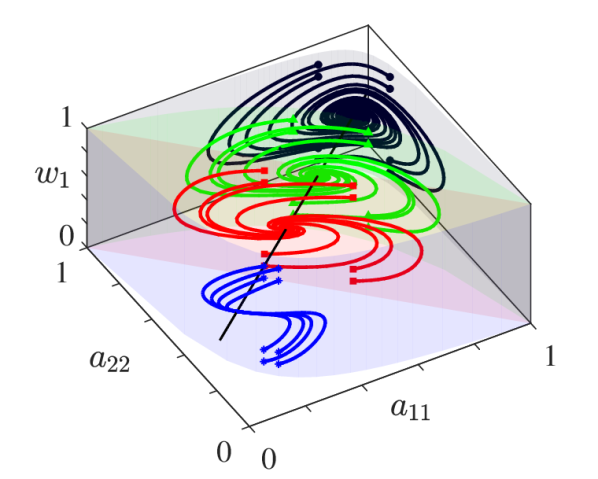
The cycle constants can be thought of as a parameter that measures the level of deviation between individual’s initial perception of each other’s skills. When $c_{r}=1$ for some $r\in\Phi(A)$ , then all individuals along cycle $r$ are in agreement over the appraisals for every other individual.

IV Stability Analysis for the ASAP Model with Donor-Controlled Work Flow

In this section, we study the asymptotic behavior of the ASAP model with donor-controlled work flow. Our analysis is based on a Lyapunov argument. Utilizing this approach, we identify initial appraisal network conditions for teams with complete graphs where the optimal workload is learned without any other additional assumptions. Under a technical assumption, we also rigorously prove that for any strongly connected team, the dynamics will converge to the optimal workload.

The next lemma defines the performance-entropy function, which we show to be a Lyapunov function for the ASAP model under certain structural assumptions on the appraisal network.

Lemma 9 (Performance-entropy function).

Consider the ASAP model (3) with donor-controlled work flow (4). Assume $A_{0}$ row-stochastic, $\bm{w}_{0}\in\mathrm{int}(\Delta_{n})$ , and there exists some $A^{*}$ with the same zero/positive pattern as $A_{0}$ such that $\bm{w}^{\mathrm{opt}}=v_{\textup{left}}(A^{*})$ . Define the performance-entropy function $V:\{a_{ij}\}_{(i,j)\in\mathcal{E}(A_{0})}\times\mathrm{int}(\Delta_{n})\rightarrow$ by

\begin{split}V(A,\bm{w})&=-\sum_{i=1}^{n}\bigg{(}\int\nolimits_{w^{\mathrm{opt}}_{i}}^{w_{i}}p_{i}(x)dx\\ &\qquad+w^{\mathrm{opt}}_{i}\sum\nolimits_{\begin{subarray}{c}k\text{ s.t.}\\ (i,k)\in\mathcal{E}(A_{0})\end{subarray}}a_{ik}^{*}\ln\Big{(}\frac{a_{ik}}{a_{ik}^{*}}\Big{)}\bigg{)}.\end{split}

(13)

Then

(i)

$V(A,\bm{w})>0$ for $A\neq A^{*}$ or $\bm{w}\neq\bm{w}^{\mathrm{opt}}$ , and
(ii)

the Lie derivative of $V$ is

$\dot{V}(A,\bm{w})=p(\bm{w})^{\top}(I_{n}-A^{\top})(\bm{w}-\bm{w}^{\mathrm{opt}}).$ (14)

The first term of the function is the rescaled total utility, $\mathcal{H}_{\textup{tot}}(\bm{w}^{\mathrm{opt}})-\mathcal{H}_{\textup{tot}}(\bm{w})=-\sum_{i=1}^{n}\int_{w^{\mathrm{opt}}_{i}}^{w_{i}}p_{i}(x)dx$ . The second term, $w^{\mathrm{opt}}_{i}\sum_{\begin{subarray}{c}k\text{ s.t.}\\ (i,k)\in\mathcal{E}(A_{0})\end{subarray}}a_{ik}^{*}\ln\frac{a_{ik}}{a_{ik}^{*}}$ , is the Kullback-Liebler relative entropy measure [25].

Proof.

By Assumption 1, $-\sum_{i=1}^{n}\int_{w^{\mathrm{opt}}_{i}}^{w_{i}}p_{i}(x)dx$ is convex with minimum value if and only if $w_{i}=w^{\mathrm{opt}}_{i}$ . Therefore this term is positive definite for $\bm{w}\neq\bm{w}^{\mathrm{opt}}$ . Since the function $-\ln(\cdot)$ is strictly convex and $\sum_{k=1}^{n}a_{ik}^{*}=1$ , Jensen’s inequality can be used to give the following lower bound,

-\sum\nolimits_{\begin{subarray}{c}k\text{ s.t.}\\ (i,k)\in\mathcal{E}(A_{0})\end{subarray}}a_{ik}^{*}\ln\Big{(}\frac{a_{ik}}{a_{ik}^{*}}\Big{)}\geq 0,

where the inequality holds strictly if and only if $A\neq A^{*}$ .

For the last statement of the lemma and with the assumption $\bm{w}^{\mathrm{opt}}=v_{\textup{left}}(A^{*})$ , the Lie derivative of $V$ is

\dot{V}(A,\bm{w})=-p(\bm{w})^{\top}\dot{\bm{w}}-(\bm{w}^{\mathrm{opt}})^{\top}\big{(}A^{*}\odot(\dot{A}\oslash A)\big{)}\mathbbold{1}_{n}\\ =-p(\bm{w})^{\top}\dot{\bm{w}}-(\bm{w}^{\mathrm{opt}})^{\top}\big{(}A^{*}\odot(\mathbbold{1}_{n}p(\bm{w})^{\top}-Ap(\bm{w})\mathbbold{1}_{n}^{\top})\big{)}\mathbbold{1}_{n}.

Then using Hadamard product property (1) and $\bm{w}^{\mathrm{opt}}=v_{\textup{left}}(A^{*})$ , $\dot{V}(A,\bm{w})$ further simplifies to

\dot{V}(A,\bm{w})=-p(\bm{w})^{\top}\dot{\bm{w}}\\ \quad-(\bm{w}^{\mathrm{opt}})^{\top}\big{(}A^{*}\operatorname{diag}(p(\bm{w}))-\operatorname{diag}(Ap(\bm{w}))A^{*}\big{)}\mathbbold{1}_{n}\\ =-p(\bm{w})^{\top}\dot{\bm{w}}-(\bm{w}^{\mathrm{opt}})^{\top}\big{(}A^{*}p(\bm{w})-Ap(\bm{w})\big{)}\\ =p(\bm{w})^{\top}(I_{n}-A^{\top})(\bm{w}-\bm{w}^{\mathrm{opt}}).\qed

The next theorem states the convergence results to the optimal workload for various cases on the connectivity of the initial appraisal matrix. For donor-controlled work flow, the optimal workload is equal to the eigenvector centrality of the network [5], which is a measure of the individual’s importance as a function of the network structure and appraisal values. Therefore the equilibrium workload value quantifies each team member’s contribution to the team and learning the optimal workload reflects the development of TMS within the team. Note that statement (iii) relies on the assumption that conjecture given in the statement holds. This conjecture is discussed further at the end of the section, where we provide extensive simulations to illustrate its high likelihood.

Theorem 10 (Convergence to optimal workload for strongly connected teams).

Consider the ASAP model (2) with donor-controlled work flow (4). Given initial conditions $A_{0}$ row-stochastic, irreducible, with strictly positive diagonal and $\bm{w}_{0}\in\mathrm{int}(\Delta_{n})$ . The following statements hold:

(i)

if $n=2$ and $A_{0}>0$ , then $\lim_{t\to\infty}\left(A(t),\bm{w}(t)\right)=(A^{*},\bm{w}^{\mathrm{opt}})$ such that $A^{*}>0$ is row-stochastic and $\bm{w}^{\mathrm{opt}}=v_{\textup{left}}(A^{*})$ ;
(ii)

if there exists $a_{d}(0)=[a_{11}(0),\dots a_{nn}(0)]^{\top}\in\mathrm{int}(\Delta_{n})$ such that $A_{0}=\mathbbold{1}_{n}a_{d}(0)^{\top}$ is also rank $1$ , then $\lim_{t\to\infty}(A(t),\bm{w}(t))=(\mathbbold{1}_{n}(\bm{w}^{\mathrm{opt}})^{\top},\bm{w}^{\mathrm{opt}})$ .

Moreover, define $\bm{v}(t)\in_{>0}^{n}$ as in Theorem 8 (iii).

(iii)

If $\bm{v}(t)$ is uniformly bounded for all $(A_{0},\bm{w}_{0})$ and $t\geq 0$ , then $\lim_{t\to\infty}(A(t),\bm{w}(t))=(A^{*},\bm{w}^{\mathrm{opt}})$ such that $A^{*}$ is row-stochastic, has the same zero/positive pattern as $A_{0}$ , and $\bm{w}^{\mathrm{opt}}=v_{\textup{left}}(A^{*})$ .

Proof.

Statement (i) follows directly from the fact that the function defined by (13) is a Lyapunov function for the system. For brevity, we omit the proof of Statement (i), since it follows a similar proof to statement (ii).

Regarding statement (ii), if $A_{0}$ is the rank $1$ form given by the theorem assumptions, then $c_{r}=1$ for all cycles $r\in\Phi(A_{0})$ by Theorem 8 (i). This implies that $a_{ij}=a_{kj}$ for any $j$ , all $i\neq k$ , and $t\geq 0$ . For the storage function $V(A,\bm{w})$ as defined by (13), the Lie derivative (14) simplifies to,

	$\displaystyle\dot{V}$	$\displaystyle=p(\bm{w})^{\top}(I_{n}-a_{d}\mathbbold{1}_{n}^{\top})\bm{w}-p(\bm{w})^{\top}(I_{n}-a_{d}\mathbbold{1}_{n}^{\top})\bm{w}^{\mathrm{opt}}$
		$\displaystyle=p(\bm{w})^{\top}(\bm{w}-a_{d}-\bm{w}^{\mathrm{opt}}+a_{d})=p(\bm{w})^{\top}(\bm{w}-\bm{w}^{\mathrm{opt}}).$

From $\bm{w},\bm{w}^{\mathrm{opt}}\in\Delta_{n}$ , then $p(\bm{w})^{\top}(\bm{w}-\bm{w}^{\mathrm{opt}})=(p(\bm{w})-p(\bm{w}^{\mathrm{opt}}))^{\top}(\bm{w}-\bm{w}^{\mathrm{opt}})=(p(\bm{w})-p^{*}\mathbbold{1}_{n})^{\top}(\bm{w}-\bm{w}^{\mathrm{opt}})$ . Since $p_{i}(w_{i})$ strictly decreasing by Assumption 1 or 2, then $\dot{V}<0$ for $\bm{w}\neq\bm{w}^{\mathrm{opt}}$ . Then $V$ is a Lyapunov function for the rank $1$ initial appraisal case and $\lim_{t\to\infty}(A(t),\bm{w}(t))=(\mathbbold{1}_{n}(\bm{w}^{\mathrm{opt}})^{\top},\bm{w}^{\mathrm{opt}})$ .

Regarding statement (iii), we start by considering the equivalent reduced order appraisal dynamics (9) and by proving asymptotic convergence using LaSalle’s Invariance Principle. Define the function $\bar{V}:_{>0}^{n}\times\mathrm{int}(\Delta_{n})\rightarrow$ , which is a modification of the storage function (13) by replacing the term $\frac{a_{ij}}{a_{ij}^{*}}$ with $v_{i}$ for all $i,j$ ,

\displaystyle\bar{V}(\bm{v},\bm{w})

\displaystyle=-\sum_{i=1}^{n}\bigg{(}\int\nolimits_{w^{\mathrm{opt}}_{i}}^{w_{i}}p_{i}(x)dx+w^{\mathrm{opt}}_{i}\ln(v_{i})\bigg{)}.

(15)

The Lie derivative of $\bar{V}$ is

	$\displaystyle\dot{\bar{V}}$	$\displaystyle=-p(\bm{w})^{\top}\dot{\bm{w}}-(\dot{\bm{v}}\oslash\bm{v})^{\top}\bm{w}^{\mathrm{opt}}$
		$\displaystyle=p(\bm{w})^{\top}(I_{n}-A^{\top})\bm{w}-\big{(}p(\bm{w})-p(\bm{w})^{\top}A^{\top}\bm{w}\mathbbold{1}_{n}\big{)}^{\top}\bm{w}^{\mathrm{opt}}$
		$\displaystyle=p(\bm{w})^{\top}(\bm{w}-\bm{w}^{\mathrm{opt}})\leq 0.$

We can now define the sublevel set $\Omega=\{\bm{v}\in_{>0}^{n},\bm{w}\in\mathrm{int}(\Delta_{n})\;|\;\bar{V}(\bm{v},\bm{w})\leq\bar{V}(\bm{v}_{0},\bm{w}_{0}),t\geq 0\}$ , which is closed and positively invariant. Note that if there exists any $i$ such that $\lim_{t\to\infty}v_{i}=0$ , then $\lim_{t\to\infty}\bar{V}(\cdot)=\infty$ . However, $\dot{\bar{V}}\leq 0$ and $\bar{V}(\bm{v}_{0},\bm{w}_{0})$ is finite, so $\bm{v}(t)$ must be bounded away from zero by a positive value for $t\geq 0$ . By our assumption, $\bm{v}(t)$ is also upper bounded. Then there exists constants $v_{\min},v_{\max}>0$ such that $\bm{v}\in[v_{\min},v_{\max}]^{n}$ . Then by LaSalle’s Invariance Principle, the trajectories must converge to the largest invariant set contained in the intersection of

\{\bm{v}\in[v_{\min},v_{\max}]^{n},\bm{w}\in\mathrm{int}(\Delta_{n})\;|\;\dot{\bar{V}}=0\}\operatorname{\cap}\Omega.

By Theorem 5, if $\dot{\bar{V}}=0$ , then $w=\bm{w}^{\mathrm{opt}}$ and $p(\bm{w}^{\mathrm{opt}})=p^{*}\mathbbold{1}_{n}$ . This implies $\dot{\bm{v}}=\operatorname{diag}(\bm{v})(p(\bm{w}^{\mathrm{opt}})-p^{*}\mathbbold{1}_{n})=0$ , so $\bm{v}=\bm{v}^{*}>0$ . By Theorem 8 (iv), $(\bm{v}^{*},\bm{w}^{\mathrm{opt}})$ corresponds to equilibrium $(A^{*},\bm{w}^{\mathrm{opt}})$ . Therefore $\lim_{t\to\infty}(\bm{v}(t),\bm{w}(t))=(\bm{v}^{*},\bm{w}^{\mathrm{opt}})$ is equivalent to $\lim_{t\to\infty}(A(t),\bm{w}(t))=(A^{*},\bm{w}^{\mathrm{opt}})$ such that $\bm{w}^{\mathrm{opt}}=v_{\textup{left}}(A^{*})$ and $A^{*}=\mathcal{A}(\bm{v}^{*})$ , where $A^{*}$ and $A_{0}$ have the same zero/positive pattern. ∎

Theorem 10 (iii) establishes asymptotic convergence from all initial conditions of interest under the assumption that the trajectory $\bm{v}(t)$ is uniformly bounded. Throughout our numerical simulation studies, we have empirically observed that this assumption has always been satisfied. We now present a Monte Carlo analysis [21] to estimate the probability that this uniform boundedness assumption holds.

For any randomly generated pair $(A_{0},\bm{w}_{0})$ , which corresponds to $\bm{v}_{0}=\mathbbold{1}_{n}$ , define the indicator function $\mathds{I}:\mathbb{R}_{\geq 0}^{n}\times\mathrm{int}(\Delta_{n})\rightarrow\{0,1\}$ as

(i)

$\mathds{I}(A_{0},\bm{w}_{0})=1$ if there exists $v_{\max}$ such that $\bm{v}(t)\leq v_{\max}\mathbbold{1}_{n}$ for all $t\in[0,1000]$ ;
(ii)

$\mathds{I}(A_{0},\bm{w}_{0})=0$ , otherwise.

Let $p=\mathds{P}[\mathds{I}(A_{0},\bm{w}_{0})=0]$ . We estimate $p$ as follows. We generate $N\in\mathbb{N}$ independent identically distributed random sample pairs, $(A_{0}^{(i)},\bm{w}_{0}^{(i)})$ for $i\in\{1,\dots,N\}$ , where $A_{0}^{(i)}\in[0,1]^{n\times n}$ is row-stochastic, irreducible, with strictly positive diagonal and $\bm{w}_{0}^{(i)}\in\mathrm{int}(\Delta_{n})$ .

Finally, we define the empirical probability as

\hat{p}_{N}=\frac{1}{N}\sum_{i=1}^{N}\mathds{I}(A_{0}^{(i)},\bm{w}_{0}^{(i)}).

For any accuracy $1-\epsilon\in(0,1)$ and confidence level $1-\xi\in(0,1)$ , then by the Chernoff Bound [21, Equation 9.14], $|\hat{p}-p|<\epsilon$ with probability greater than confidence level $1-\xi$ if

N\geq\frac{1}{2\epsilon^{2}}\log\frac{2}{\xi}.

(16)

For $\epsilon=\xi=0.01$ , the Chernoff bound (16) is satisfied by $N=27\,000$ .

Our simulation setup is as follows. We run $27\,000$ independent MATLAB simulations for the ASAP model (2) with donor-controlled work flow (5). We consider $n=6$ , irreducible with strictly positive diagonal $A_{0}$ generated using the Erdös-Renyi random graph model with edge connectivity probability $0.3$ , and performance functions of the form $p_{i}(w_{i})=(\frac{s_{i}}{w_{i}})^{\gamma_{i}}$ for $\gamma_{i}\in(0,1)$ and $[s_{1},\dots,s_{n}]\in\mathrm{int}(\Delta_{n})$ . We find that $\hat{p}_{N}=1$ . Therefore, we can make the following statement.
Consider (i) $n=6$ ; (ii) $A_{0}$ irreducible with strictly positive diagonal generated by the Erdös-Renyi random graph model with edge connectivity probability $0.3$ , and randomly generated edge weights normalized to be row-stochastic; and (iii) $\bm{w}_{0}\in\mathrm{int}(\Delta_{n})$ . Then with $99\%$ confidence level, there is at least $0.99\%$ probability that $\left\|{\bm{v}(t)}\right\|$ is uniformly upper bounded for $t\in[0,1000]$ .

V Stability Analysis for the ASAP Model with Average-Appraisal Work Flow

This section investigates the asymptotic behavior of the ASAP model (2) with average-appraisal work flow (5). In contrast with the eigenvector centrality model, we observe that strongly connected teams obeying this work flow model are not always able to learn their optimal work assignment. First we give a necessary condition on the initial appraisal matrix and optimal work assignment for convergence to the optimal team performance. Second, we prove that learning the optimal work assignment can be guaranteed if the team has a complete network topology or if the collective team performance is optimized by an equally distributed workload. Note that the results in Sections II-III also hold for average-appraisal work flow, only if the equilibrium satisfies $\bm{w}^{\mathrm{opt}}=\frac{1}{n}(A^{*})^{\top}\mathbbold{1}_{n}$ .

Let $\lceil x\rceil$ denote the ceiling function which rounds up all elements of $x$ to the nearest integer. The following lemma gives a condition that guarantees when the team is unable to learn the optimal workload assignment.

Lemma 11 (Condition for failure to learn optimal work assignment for the degree centrality model).

Consider the ASAP model (2) with average-appraisal work flow (5). Assume $A_{0}$ row-stochastic and $\bm{w}_{0}\in\mathrm{int}(\Delta_{n})$ . If there exists at least one $i\in\{1,\dots,n\}$ such that $w^{\mathrm{opt}}_{i}>\max\{\frac{1}{n}\sum_{k=1}^{n}\lceil a_{ki}(0)\rceil,w_{i}(0)\}$ . Then $\bm{w}(t)\neq\bm{w}^{\mathrm{opt}}$ for any $t\geq 0$ .

Proof.

By the Grönwall-Bellman Comparison Lemma, $\dot{w}_{i}\leq-w_{i}+\frac{1}{n}\sum_{k=1}^{n}\lceil a_{ki}(0)\rceil$ implies that

	$\displaystyle w_{i}(t)$	$\displaystyle\leq-w_{i}(0)e^{-t}+\frac{1}{n}\sum\nolimits_{k=1}^{n}\lceil a_{ki}(0)\rceil(e^{-t}-1)$
		$\displaystyle\leq\max\Big{\{}\frac{1}{n}\sum\nolimits_{k=1}^{n}\lceil a_{ki}(0)\rceil,w_{i}(0)\Big{\}}.$

Therefore if there exists at least one $i$ such that $w^{\mathrm{opt}}_{i}>\max\{\frac{1}{n}\sum_{k=1}^{n}\lceil a_{ki}(0)\rceil,w_{i}(0)\}$ , then $w_{i}(t)\neq w^{\mathrm{opt}}_{i}$ . ∎

This sufficient condition for failure to learn the optimal workload can also be stated as a necessary condition for learning the optimal workload. In other words, if $\lim_{t\to\infty}\bm{w}(t)=\bm{w}^{\mathrm{opt}}$ , then $\bm{w}^{\mathrm{opt}}_{i}\leq\max\{\frac{1}{n}\sum_{k=1}^{n}\lceil a_{ki}(0)\rceil,w_{i}(0)\}$ for all $i$ .

While the average-appraisal work flow does not converge to the optimal equilibrium for strongly connected teams and general initial conditions, the following lemma describes two cases that do guarantee learning of the optimal workload.

Lemma 12 (Convergence to optimal workload for average-appraisal work flow).

Consider the ASAP model (2) with average-appraisal work flow (5). The following statements hold.

(i)

If $A_{0}$ is row-stochastic, irreducible, with strictly positive diagonal, $\bm{w}(0)\in\mathrm{int}(\Delta_{n})$ , and $\bm{w}^{\mathrm{opt}}=\frac{1}{n}\mathbbold{1}_{n}$ , then $\lim_{t\to\infty}(A(t),\bm{w}(t))=(A^{*},\frac{1}{n}\mathbbold{1}_{n})$ where $A^{*}$ has the same zero/positive pattern as $A_{0}$ and is doubly-stochastic with $\frac{1}{n}(A^{*})^{\top}\mathbbold{1}_{n}=\frac{1}{n}\mathbbold{1}_{n}$ ;
(ii)

if $A_{0}>0$ is row-stochastic and $\bm{w}(0)\in\mathrm{int}(\Delta_{n})$ , then $\lim_{t\to\infty}(A(t),\bm{w}(t))=(A^{*},\bm{w}^{\mathrm{opt}})$ where $A^{*}>0$ and $\bm{w}^{\mathrm{opt}}=\frac{1}{n}(A^{*})^{\top}\mathbbold{1}_{n}$ .

Proof.

Regarding statement (i), the storage function from (13) is a Lyapunov function for the given dynamics with assumption $\bm{w}^{\mathrm{opt}}=\frac{1}{n}\mathbbold{1}_{n}=\frac{1}{n}(A^{*})^{\top}\mathbbold{1}_{n}$ . The Lie derivative $\dot{V}$ is

\dot{V}(A,\bm{w})=-p(\bm{w})^{\top}\dot{\bm{w}}-(\bm{w}^{\mathrm{opt}})^{\top}(A^{*}-A)p(\bm{w}).\\ =p(\bm{w})^{\top}\Big{(}\bm{w}-\frac{1}{n}A^{\top}\mathbbold{1}_{n}-\frac{1}{n}(A^{*})^{\top}\mathbbold{1}_{n}+\frac{1}{n}A^{\top}\mathbbold{1}_{n}\Big{)}\\ =p(\bm{w})^{\top}(\bm{w}-\bm{w}^{\mathrm{opt}})\leq 0.

By Lemma 9, $V=0$ if and only if $\bm{w}=\bm{w}^{\mathrm{opt}}=\frac{1}{n}\mathbbold{1}_{n}$ and $A=A^{*}$ such that $\frac{1}{n}(A^{*})^{\top}\mathbbold{1}_{n}=\frac{1}{n}\mathbbold{1}_{n}$ . Therefore $\lim_{t\to\infty}(A(t),\bm{w}(t))=(A^{*},\frac{1}{n}\mathbbold{1}_{n})$ where $A_{0}$ and $A^{*}$ have the same zero/positive pattern.

Regarding statement (ii), consider the reduced order dynamics (9), with $\tilde{p}(\bm{v},\bm{w})=\bm{w}^{\top}\mathcal{A}(\bm{v})p(\bm{w})$ for shorthand. Define the function $\bar{V}:_{>0}^{n}\times\mathrm{int}(\Delta_{n})\rightarrow$ as where

\bar{V}(\bm{v},\bm{w})=\sum_{i=1}^{n}\bigg{(}-\int\nolimits_{w^{\mathrm{opt}}_{i}}^{w_{i}}p_{i}(x)dx\\ -w^{\mathrm{opt}}_{i}\ln(v_{i})+\frac{1}{n}\ln\Big{(}\sum\nolimits_{k=1}^{n}a_{ik}(0)v_{k}\Big{)}\bigg{)}.

First, we show that $\bar{V}$ is lower bounded. Second, we illustrate that $\bar{V}$ is monotonically decreasing for $\bm{w}\neq\bm{w}^{\mathrm{opt}}$ . Then this allows us to show convergence to an optimal equilibrium.

Let $a_{\min}=\min_{i,j}\{a_{ij}(0)\}$ . From the proof of Lemma 9, $-\int\nolimits_{w^{\mathrm{opt}}_{i}}^{w_{i}}p_{i}(x)dx\geq 0$ for all $i$ . Then $\bar{V}$ is lower bounded by

	$\displaystyle\bar{V}$	$\displaystyle\geq-\sum_{i=1}^{n}\bigg{(}w^{\mathrm{opt}}_{i}\ln(v_{i})+\frac{1}{n}\ln\Big{(}\frac{1}{a_{\min}\left\\|{\bm{v}}\right\\|_{1}}\Big{)}\bigg{)}$
		$\displaystyle\geq\ln(a_{\min})-\sum_{i=1}^{n}w^{\mathrm{opt}}_{i}\ln\Big{(}\frac{v_{i}}{\left\\|{\bm{v}}\right\\|_{1}}\Big{)}\geq\ln(a_{\min}).$

Now we show that $\dot{\bar{V}}\leq 0$ . Define the function $\bm{u}:_{>0}^{n}\rightarrow_{>0}^{n}$ , where $\bm{u}(\bm{v})=\operatorname{diag}(A_{0}\bm{v})^{-1}$ , which reads element-wise as $u_{i}(\bm{v})=\sum\nolimits_{k=1}^{n}a_{ik}(0)v_{k}$ . Using $A(t)=\mathcal{A}(\bm{v}(t))$ as in (10), then the rate of change of $\bm{u}$ is given by

\dot{\bm{u}}=-\operatorname{diag}(\bm{u})^{2}A_{0}\dot{\bm{v}}=-\operatorname{diag}(\bm{u})\big{(}Ap(\bm{w})-\tilde{p}(\bm{v},\bm{w})\mathbbold{1}_{n}\big{)}.

Plugging $\bm{u}$ into $\bar{V}$ , the Lie derivative of $\bar{V}$ is

\dot{\bar{V}}(\bm{v},\bm{w})=-p(\bm{w})^{\top}\dot{\bm{w}}-(\dot{\bm{v}}\oslash\bm{v})^{\top}\bm{\bm{w}^{\mathrm{opt}}}-\frac{1}{n}(\dot{\bm{u}}\oslash\bm{u})^{\top}\mathbbold{1}_{n}\\ =-p(\bm{w})^{\top}(-\bm{w}+\frac{1}{n}A^{\top}\mathbbold{1}_{n})-(p(\bm{w})-\tilde{p}(\bm{v},\bm{w})\mathbbold{1}_{n})^{\top}\bm{w}^{\mathrm{opt}}\\ -\frac{1}{n}(-Ap(\bm{w})+\tilde{p}(\bm{v},\bm{w})\mathbbold{1}_{n})^{\top}\mathbbold{1}_{n}\\ =p(\bm{w})^{\top}\big{(}\bm{w}-\bm{w}^{\mathrm{opt}}\big{)}+\tilde{p}(\bm{v},\bm{w})\big{(}\mathbbold{1}_{n}^{\top}\bm{w}^{\mathrm{opt}}-\frac{1}{n}\mathbbold{1}_{n}^{\top}\mathbbold{1}_{n}\big{)}\\ =p(\bm{w})^{\top}(\bm{w}-\bm{w}^{\mathrm{opt}})\leq 0.

Since $\dot{\bar{V}}\leq 0$ , implies that $\bar{V}(\bm{v},\bm{w})\leq\bar{V}(\bm{v}_{0},\bm{w}_{0})<\infty$ , we can conclude that there exists some strictly positive constant $v_{\min}>0$ such that $\bm{v}\geq v_{\min}\mathbbold{1}_{n}$ .

Note that $\dot{\bar{V}}=0$ if and only if $\bm{w}=\bm{w}^{\mathrm{opt}}$ by Lemma 9. Because $\bar{V}$ has a finite lower bound and is monotonically decreasing for $\bm{w}\neq\bm{w}^{\mathrm{opt}}$ , then as $t\to\infty$ , $\bar{V}$ will decrease to the level set where $\bm{w}=\bm{w}^{\mathrm{opt}}$ . Then $\bm{w}=\bm{w}^{\mathrm{opt}}$ implies $\dot{\bm{w}}=0$ and $\dot{\bm{v}}=0$ . Therefore $\lim_{t\to\infty}(\bm{v},\bm{w})=(\bm{v}^{*},\bm{w}^{\mathrm{opt}})$ such that $\bm{w}^{\mathrm{opt}}=\frac{1}{n}\mathcal{A}(\bm{v}^{*})^{\top}\mathbbold{1}_{n}=\frac{1}{n}(A^{*})^{\top}\mathbbold{1}_{n}$ . ∎

VI Numerical Simulations

In this section, we utilize numerical simulations to investigate various cases of the ASAP model to illustrate when teams succeed and fail at optimizing their collective performance.

For all the simulations in this section, we consider performance functions of the form $p_{i}(w_{i})=(\frac{s_{i}}{w_{i}})^{\gamma}$ for $\gamma\in(0,1)$ and all $i$ , which satisfy Assumptions 1-2. Then the same optimal workload maximizes any choice of collective team performance we have introduced.

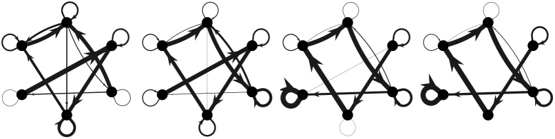
First, we provide an example of a team with a strongly connected appraisal network and strictly positive self-appraisal weights, i.e. satisfying the assumptions of Theorem 10 (iii), to illustrate a case where the team learns the optimal work assignment. Figure 3 illustrates the evolution of the appraisal network and work assignment of the ASAP model (2) with donor-controlled work flow (4).

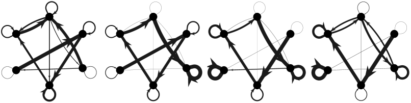
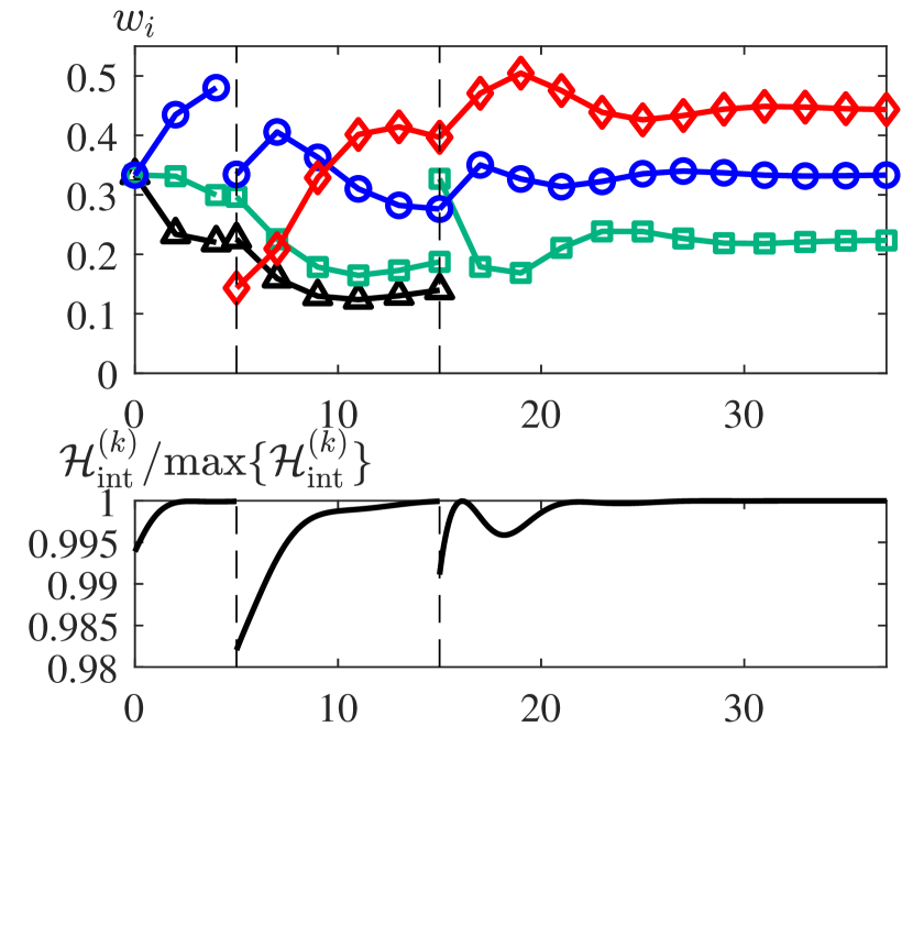
VI-A Distributed optimization illustrated with switching team members

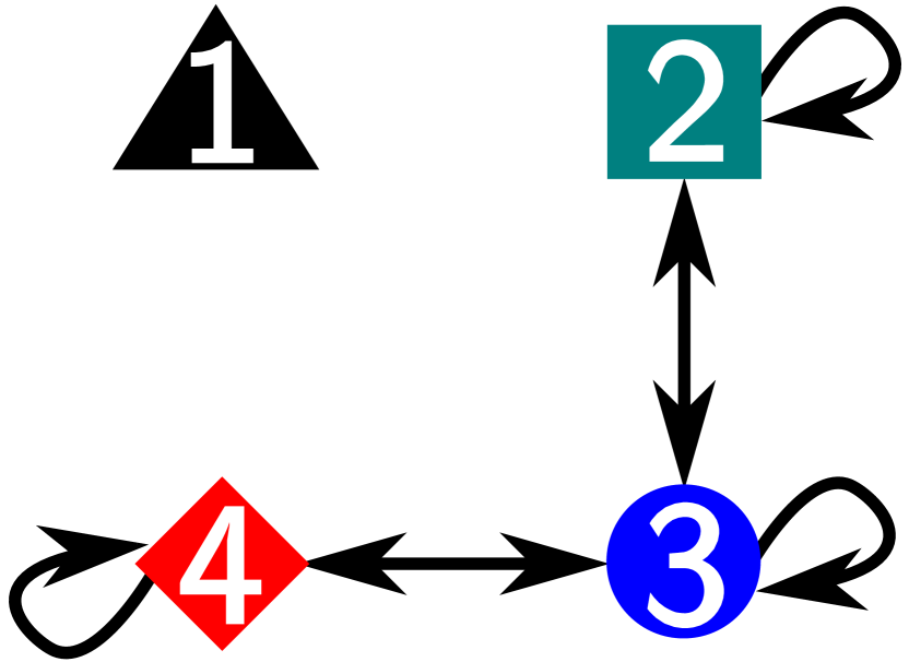
Next we consider another example of the ASAP model (2) with donor-controlled work flow (4), where individuals are switching in and out of the team. Under the behavior governed by the ASAP model, only affected neighboring individuals need to be aware of an addition or subtraction of a team member, since the model is both distributed and decentralized. In this example, when individual $j$ is added to the team as a neighbor of individual $i$ , $i$ allocates a portion of their work assignment to the new individual $j$ . Similarly, if individual $j$ is removed, then $j$ ’s neighbors will absorb $j$ ’s workload. Let $k=1$ , $k=2$ , and $k=3$ denote the subteams from time intervals $t\in[0,5)$ , $t\in[5,15)$ , and $t\in[15,\infty)$ , respectively. Then let $\mathcal{H}_{\textup{tot}}^{(k)}$ denote the collective performance for the $k$ th subteam. Figure 4 illustrates the appraisal network topologies of each subteam and the evolution of the workload $\bm{w}(t)$ and normalized collective team performance $\mathcal{H}_{\textup{tot}}^{(k)}$ .

VI-B Failure to learn

Partial observation of performance feedback does not guarantee learning optimal work assignment

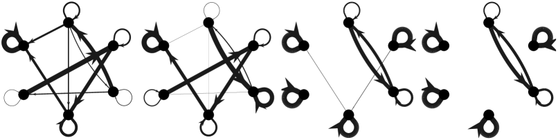
Partial observation occurs when the appraisal network does not have the desired strongly connected property, resulting in team members having insufficient feedback to determine their optimal work assignment. We consider an example of the ASAP model (2) with donor-controlled work flow (4) and reducible initial appraisal network $A_{0}$ . Figure 5(a) illustrates how some appraisal weights between neighboring individuals approach zero asymptotically, resulting in the team not being capable of learning the work distribution that maximizes the collective team performance.

Average-appraisal feedback limits direct cooperation

Figure 5(b) is an example of a team obeying the ASAP model (2) with average-appraisal work flow (5). Even if the team does not satisfy the sufficient conditions for failure from Lemma 11, when individuals adjust their work assignment with only their average-appraisal as the input, the team may still not succeed in learning the correct workload to maximize the team performance.

VII Conclusion

This paper proposes novel models for the evolution of interpersonal appraisals and the assignment of workload in a team of individuals engaged in a sequence of tasks. We propose appraisal networks as a mathematical multi-agent model for the applied psychological concept of TMS. For two natural models of workload assignment, we establish conditions under which a correct TMS develops and allows the team to achieve optimal workload assignment and optimal performance. Our two proposed workload assignment mechanisms feature different degrees of coordination among team members. The donor-controlled work flow model requires a higher level of coordination compared to the average-appraisal work flow and, as a result, achieves optimal behavior under weaker requirements on the initial appraisal matrix.

Possible future research directions include studying team’s behavior when individuals in the team update their appraisals and work assignments asynchronously. The updates could be modeled using an additional contact network with switching topology. More investigation can also be done to determine if it is possible to predict which appraisal weights in a weakly connected network approach zero asymptotically, using only information on the initial work distribution and appraisal values.

VIII Code Availability

The source code is publicly available under https://github.com/eyhuang66/assign-appraise-dynamics-of-teams.

References

[1] E. G. Anderson Jr and K. Lewis. A dynamic model of individual and collective learning amid disruption. Organization Science, 25(2):356–376, 2014. doi:10.1287/orsc.2013.0854.
[2] J. Barreiro-Gomez, G. Obando, and N. Quijano. Distributed population dynamics: Optimization and control applications. IEEE Transactions on Systems, Man, and Cybernetics: Systems, 47(2):304–314, 2016. doi:10.1109/TSMC.2016.2523934.
[3] P. Bauer. A sequential elimination procedure for choosing the best population(s) based on multiple testing. Journal of Statistical Planning and Inference, 21(2):245–252, 1989. doi:10.1016/0378-3758(89)90008-6.
[4] C. Berge. Graphs and Hypergraphs. North-Holland, 1973, ISBN 072042450X.
[5] P. Bonacich. Power and centrality: A family of measures. American Journal of Sociology, 92(5):1170–1182, 1987. doi:10.1086/228631.
[6] F. Bullo. Lectures on Network Systems. Kindle Direct Publishing, 1.4 edition, July 2020, ISBN 978-1986425643. With contributions by J. Cortés, F. Dörfler, and S. Martínez. URL: http://motion.me.ucsb.edu/book-lns.
[7] N. E. Friedkin. A formal theory of reflected appraisals in the evolution of power. Administrative Science Quarterly, 56(4):501–529, 2011. doi:10.1177/0001839212441349.
[8] L. Gong, J. Gao, and M. Cao. Evolutionary game dynamics for two interacting populations in a co-evolving environment. In IEEE Conf. on Decision and Control, pages 3535–3540, 2018. doi:10.1109/CDC.2018.8619801.
[9] A. C. Graesser, S. M. Fiore, S. Greiff, J. Andrews-Todd, P. W. Foltz, and F. W. Hesse. Advancing the science of collaborative problem solving. Psychological Science in the Public Interest, 19(2):59–92, 2018. doi:10.1177/1529100618808244.
[10] J. A. Grand, M. T. Braun, G. Kuljanin, S. W. J. Kozlowski, and G. T. Chao. The dynamics of team cognition: A process-oriented theory of knowledge emergence in teams. Journal of Applied Psychology, 101(10):1353–1385, 2016. doi:10.1037/apl0000136.
[11] T. Gross and B. Blasius. Adaptive coevolutionary networks: A review. Journal of The Royal Society Interface, 5(20):259–271, 2008. doi:10.1098/rsif.2007.1229.
[12] J. Hofbauer and K. Sigmund. Evolutionary Games and Population Dynamics. Cambridge University Press, 1998, ISBN 052162570X.
[13] C. Hsiung. The effectiveness of cooperative learning. Journal of Engineering Education, 101(1):119–137, 2012. doi:10.1002/j.2168-9830.2012.tb00044.x.
[14] J. A. Jacquez and C. P. Simon. Qualitative theory of compartmental systems. SIAM Review, 35(1):43–79, 1993. doi:10.1137/1035003.
[15] S. W. J. Kozlowski, W. J. Steve, and B. S. Bell. Evidence-based principles and strategies for optimizing team functioning and performance in science teams. In Strategies for Team Science Success, pages 269–293. Springer, 2019. doi:10.1007/978-3-030-20992-6_21.
[16] W. Mei, N. E. Friedkin, K. Lewis, and F. Bullo. Dynamic models of appraisal networks explaining collective learning. IEEE Transactions on Automatic Control, 63(9):2898–2912, 2018. doi:10.1109/TAC.2017.2775963.
[17] A. Nedić, A. Ozdaglar, and P. A. Parrilo. Constrained consensus and optimization in multi-agent networks. IEEE Transactions on Automatic Control, 55(4):922–938, 2010. doi:10.1109/TAC.2010.2041686.
[18] A. Newell and P. S. Rosenbloom. Mechanisms of skill acquisition and the law of practice. In J. R. Anderson, editor, Cognitive Skills and Their Acquisition, volume 1, pages 1–55. Taylor & Francis, 1981.
[19] M. Ogura and V. M. Preciado. Stability of spreading processes over time-varying large-scale networks. IEEE Transactions on Network Science and Engineering, 3:44–57, 2016. doi:10.1109/TNSE.2016.2516346.
[20] S. Ryan and R. V. O’Connor. Acquiring and sharing tacit knowledge in software development teams: An empirical study. Information and Software Technology, 55(9):1614–1624, 2013. doi:10.1016/j.infsof.2013.02.013.
[21] R. Tempo, G. Calafiore, and F. Dabbene. Randomized Algorithms for Analysis and Control of Uncertain Systems. Springer, 2005, ISBN 1-85233-524-6.
[22] Z. Wang, M. A. Andrews, Z. X. Wu, L. Wang, and C. T. Bauch. Coupled disease-behavior dynamics on complex networks: A review. Physics of Life Reviews, 15:1–29, 2015. doi:10.1016/j.plrev.2015.07.006.
[23] D. M. Wegner. Transactive memory: A contemporary analysis of the group mind. In B. Mullen and G. R. Goethals, editors, Theories of Group Behavior, pages 185–208. Springer, 1987. doi:10.1007/978-1-4612-4634-3_9.
[24] E. Wei, A. Ozdaglar, and A. Jadbabaie. A distributed Newton method for network utility maximization, I: Algorithm. IEEE Transactions on Automatic Control, 58(9):2162–2175, 2013. doi:10.1109/TAC.2013.2253218.
[25] J. W. Weibull. Evolutionary Game Theory. MIT Press, 1997, ISBN 9780262731218.
[26] J. S. Weitz, C. Eksin, S. P. Brown K. Paarporn, and W. C. Ratcliff. An oscillating tragedy of the commons in replicator dynamics with game-environment feedback. Proceedings of the National Academy of Sciences, 113(47):E7518–E7525, 2016. doi:10.1073/pnas.1604096113.

Francesco Bullo (S’95-M’99-SM’03-F’10) is a Professor with the Mechanical Engineering Department and the Center for Control, Dynamical Systems and Computation at the University of California, Santa Barbara. He was previously associated with the University of Padova (Laurea degree in Electrical Engineering, 1994), the California Institute of Technology (Ph.D. degree in Control and Dynamical Systems, 1999), and the University of Illinois. He served on the editorial boards of IEEE, SIAM, and ESAIM journals and as IEEE CSS President. His research interests focus on network systems and distributed control with application to robotic coordination, power grids and social networks. He is the coauthor of “Geometric Control of Mechanical Systems” (Springer, 2004), “Distributed Control of Robotic Networks” (Princeton, 2009), and “Lectures on Network Systems” (Kindle Direct Publishing, 2019, v1.3). He received best paper awards for his work in IEEE Control Systems, Automatica, SIAM Journal on Control and Optimization, IEEE Transactions on Circuits and Systems, and IEEE Transactions on Control of Network Systems. He is a Fellow of IEEE, IFAC, and SIAM.