Asymmetric Quantum Concatenated and Tensor Product Codes with Large -Distances
Abstract
In this paper, we present a new construction of asymmetric quantum codes (AQCs) by combining classical concatenated codes (CCs) with tensor product codes (TPCs), called asymmetric quantum concatenated and tensor product codes (AQCTPCs) which have the following three advantages. First, only the outer codes in AQCTPCs need to satisfy the orthogonal constraint in quantum codes, and any classical linear code can be used for the inner, which makes AQCTPCs very easy to construct. Second, most AQCTPCs are highly degenerate, which means they can correct many more errors than their classical TPC counterparts. Consequently, we construct several families of AQCs with better parameters than known results in the literature. Third, AQCTPCs can be efficiently decoded although they are degenerate, provided that the inner and outer codes are efficiently decodable. In particular, we significantly reduce the inner decoding complexity of TPCs from to by considering error degeneracy, where and are the block length of the inner code and the outer code, respectively. Furthermore, we generalize our concatenation scheme by using the generalized CCs and TPCs correspondingly.
Index Terms:
Asymmetric quantum code, concatenated code, error degeneracy, tensor product code.I Introduction
Quantum noise due to decoherence widely exists in quantum communication channels, quantum gates and quantum measurement. It is one of the biggest challenges in realizing large-scale quantum communication systems and fully fault-tolerant quantum computation. For a quantum state, the two main mechanisms of decoherence are population relaxation and dephasing. The level of noise is usually characterized by the relaxation time and the dephasing time . Further, dephaisng usually generates a single phase flip error, while population relaxation generates a mixed bit-phase flip error. It is shown in almost all quantum systems that, the dephasing rate is much faster than the relaxation rate , i.e., [1, 2]. For example, in the trapped ions [1, 3], the ratio can be larger than and, in quantum dots systems [4], it can be larger than . Such large asymmetry between population relaxation and dephasing indicates that phase flip errors (-errors) happen much more frequently than bit flip errors (-errors).
Steane first saw that prior knowledge of this asymmetry in errors could be leveraged for performance gains and, hence, proposed asymmetric quantum codes (AQCs) in [5]. In the years since, many AQCs have been designed to have a biased error correction towards -errors [1, 6, 7, 8]. For example, AQCs constructed from classical Bose-Chaudhuri-Hocquenghem (BCH) codes [9] and low-density parity-check (LDPC) codes [10, 11, 12, 13, 14] were proposed in [1, 7]. The BCH codes are used to correct -errors and the more powerful LDPC codes are used to correct -errors. Another approach, devised by Galindo et al. [15], is to introduce some preshared entanglement [16, 17, 18, 19, 20, 21] to help construct AQCs. More recently, asymmetric errors have been explored as a way to help improve the fault-tolerant thresholds [6, 8], particularly, in topological quantum codes [2, 22, 23]. In [8], a family of asymmetric Bacon-Shor (ABS) codes with parameters , where and are positive integers, is used for fault-tolerant quantum computation against highly biased noise. For example, ABS codes with parameters and can achieve a very low logical error rate around with much fewer physical two-qubit gates than symmetric quantum codes. In [22], surface codes definied on a square lattice of qubits with and have thresholds exceeding when the asymmetry between -errors and -errors is around . Even more, it is shown recently in [24] that thresholds for surface codes can exceed the zero-rate Shannon bound of Pauli channels when the asymmetry is properly large! These results reveal that the large asymmetry in quantum channels has a significant effect to quantum error correction and needs to be further exploited.
However, although there are many different constructions of AQCs in the literature, only a few are made on binary AQCs with a relatively large -distance . This is because the dual-containing constraint in CSS codes often makes constructing an AQC with a large minimum distance difficult. Aly [25] and Sarvepalli et al. [7] derived families of binary asymmetric quantum Bose-Chaudhuri-Hocquenghemmds (QBCH) codes with minimum distances and , both upper bounded by the square root of the block length. Li et al. [26] were able to construct a few binary QBCH codes of length with a large minimum distance . Ezerman et al. [27] constructed some binary CSS-like AQCs of length with best-known parameters by exhaustively searching the database of MAGMA [28]. Additionally, several families of nonbinary AQCs with a large have been developed, but all have a large field size [29, 30, 31].
The key to construct an AQC is to find two classical linear codes that satisfy a certain dual-containing relationship. In classical codes, the two most useful combining methods for constructing linear codes from short constituent codes are: concatenated codes (CCs) [32] and tensor product codes (TPCs) [33, 34]. In general, CCs have a large minimum distance because the distances in the constituent codes are multiplied, while TPCs have a poor minimum distance but a better dimension as a trade-off. In [35], Maucher et al. show that generalized concatenated codes (GCCs) are equivalent to generalized tensor product codes (GTPCs).
It is not difficult to apply the concatenation method to the quantum realm, i.e., to construct concatenated quantum codes (CQCs) [36, 37] and quantum tensor product codes (QTPCs) [38, 39], including asymmetric QTPCs [40] and entanglement-assisted QTPCs [41]. CQCs and QTPCs also exhibit some similar characteristics to their classical counterparts. For example, CQCs have a large minimum distance but a relatively small dimension, which is seeing them play an important role in fault-tolerant quantum computation. And, like TPCs, QTPCs have a large dimension but a small minimum distance. However, it is worth noting that CQCs are not constructed from classical CCs directly, but rather by serially concatenating two constituent quantum codes. This means both the inner and outer constituent codes need to satisfy the dual-containing relationship, which limits their construction. The same does not apply to QTPCs, giving them a distinct advantage. But QTPCs usually have a poor minimum distance. Moreover, some CQCs are known to be degenerate codes [37], which is a unique phenomenon in quantum coding theory. Degenerate codes have an advantage in that they can correct more errors than non-degenerate codes, but, in general, they are difficult to decode (see [42]) with the classical decoding algorithms often failing outright.
Hence, in this paper, we propose a novel concatenation scheme called asymmetric quantum concatenated and tensor product codes (AQCTPCs) that combines both CCs and TPCs, where CCs are used to correct -errors, and TPCs are used to correct -errors. Compared to the current methods, this new concatenation scheme has several advantages.
-
1)
In AQCTPCs, only the outer constituent codes over the extension field need to satisfy the dual-containing constraint. The inner constituent codes can be any classical linear codes. Then we have much freedom in the choice of the constituent codes.
-
2)
It is shown that AQCTPCs can be decoded efficiently provided that the classical constituent codes can be decoded efficiently. In addition, AQCTPCs are highly degenerate for correcting -errors and they can correct many more -errors beyond the error correction ability of the corresponding TPCs. Further, we show that the total inner decoding complexity of TPCs is reduced significantly from to due to error degeneracy. To this end, we have developed a syndrome-based decoding algorithm specifically for AQCTPCs.
-
3)
The AQCTPCs demonstrated in this paper are better than QBCH codes or asymmetric quantum algebraic geometry (QAG) codes as the block length goes to infinity. We construct a family of AQCTPCs with a very large -distance , of approximately half the block length. Meanwhile, the dimension and the -distance continue increasing as the block length goes to infinity. If , then the -distance is larger than half the block length.
We compare the parameters of AQCTPCs to previous results, and provide a generalized AQCTPC concatenation scheme that uses GCCs and GTPCs. We list AQCTPCs with better parameters than the binary extension of asymmetric quantum Reed-Solomon (QRS) codes. We derive families of AQCTPCs with the largest -distance compared to existed AQCs with comparable block length and -distance .
The rest of this paper is organized as follows. In Section II, we provide the basic notations and definitions needed for the construction of AQCTPCs. In Section III, we present the AQCTPC concatenation scheme and the decoding algorithms. Section IV provides detailed performance comparisons of AQCTPCs against previous constructions, and the discussions and conclusions follow in Section V.
II Preliminaries
In this section we first review some basic definitions and known results about stabilizer codes and AQCs, followed by the introduction of classical CCs and TPCs and their generalizations.
II-A Stabilizer Codes and Asymmetric Quantum Codes
Denote by a power of a prime and denote by the prime field. Let be the finite field with elements and let the field be a field extension of , where is an integer. Let be the field of complex numbers. For a positive integer , let be the th tensor product of . Denote by and two vectors of . Define the error operators on by and , where “” stands for the trace operation from to , and is a primitive th root of unity. Denote by
| (1) |
the group generated by . For any , where and , the weight of is defined by
| (2) |
The weight of -errors and the weight of -errors in are defined by and , respectively, where “” stands for the Hamming weight. The definition of quantum stabilizer codes is given below.
Definition II.1
A -ary quantum stabilizer code is a -dimensional () subspace of such that
| (3) |
where is a subgroup of and is called the stabilizer group. has minimum distance if it can detect all errors of weight up to . Then is denoted by . Further, is called non-degenerate if each stabilizer in has quantum weight at least the minimum distance , otherwise it is degenerate.
The Calderbank-Shor-Steane (CSS) code in [43, 5] is a special family of quantum stabilizer codes and can be constructed from two classical linear codes which satisfy some dual-containing relationship. Let and be two positive integers. We define an AQC as a CSS code in with parameters if it can detect all of weight up to and weight up to , simultaneously. The construction in [7, 1, 44] can be used to construct AQCs in which a pair of classical linear codes are used, one for correcting -errors and the other for correcting -errors.
Lemma II.1 ([44, Theorem 2.4])
Let and be two classical linear codes with parameters and , respectively, and . Then there exists an AQC with parameters where
| (4) |
| (5) |
If and , then is non-degenerate, otherwise it is degenerate.
II-B Classical Tensor Product Codes
Let be a classical linear code whose parity check matrix is given by , and let be the number of parity checks. Let be a linear code over the extension field whose parity check matrix is given by . Let . Denote by
| (6) |
the tensor product code of and . The block length and dimension of are given by . In addition, and are known as the inner and outer constituent codes of , respectively. If we regard as a matrix with elements over , then the parity check matrix of is the Kronecker product of and , i.e.,
| (7) |
Then we can derive a parity check matrix of with elements over by expanding all the elements of from to . The error detection/correction ability of is restricted by the constituent codes and is given by:
Lemma II.2 ([33, Theorem 1])
Partition the codeword of into sub-blocks, where each sub-block contains elements, and assume that the constituent code can detect or correct an error pattern class ( or 2), then the TPC can detect or correct all error-patterns where the sub-blocks containing errors form a pattern belonging to class and the errors within each erroneous sub-block fall within the class .
Here we give an illustrative example for the construction of TPCs.
Example II.1
Let be a binary repetition code with a parity check matrix given by
| (11) |
where is a primitive element of such that . Let be a -ary linear code over , such as we let be a maximum-distance-separable (MDS) code with a parity check matrix
| (12) |
Then we can derive a TPC of length whose parity check matrix is given in (20).
| (15) | |||||
| (20) |
Ref. [35] shows that the parity check matrix of TPCs can also be represented in a companion matrix form. Let be a primitive polynomial over and denote by a primitive element of . The companion matrix of is defined to be the matrix
| (21) |
Then for any element of , the companion matrix of , denoted by , is an matrix with elements over . Let the parity check matrix of the constituent code be with elements over , i.e., for and . Following the notations used in [35], we denote by , where is a companion matrix form. The parity check matrix of can be written as
| (26) | |||||
in which the matrix is obtained by transposing the constituent companion matrices of , and is the transpose of . According to [35, 45], if we do not transpose the constituent companion matrices in (26), we can obtain another representation of the parity check matrix as follows
| (31) | |||||
The two representations in (26) and (31) do not make any difference for the parameters and the error correction performance of TPCs. We will use them alternately in the following constructions. It should be noticed that the Kronecker product defined in equations (26) and (31) is a little different from the standard one. In the following, the Kronecker product of matrices follows the definition in (26) and (31).
The generalized tensor product codes are proposed in [35, 46] by combining a series of outer codes and inner codes. Let and be pairs of inner and outer codes, respectively, where and . Let the parity check matrices of and , respectively, be and , . Assume that all the rows in , , are independent with each other. Then the parity check matrix of the GTPCs
| (32) |
is defined by
| (33) |
where is obtained by transposing the component companion matrices of for each . The block length and the dimension of GTPCs are given by , where for .
II-C Classical Concatenated Codes
Concatenated codes can be seen as the dual counterpart of TPCs, which are obtained by concatenating an inner code with an outer code . Denote the concatenation of and by
| (34) |
and (see [9, 32]). The generator matrix of can also be given in a companion matrix form (see [35])
| (35) |
where and are the generator matrices of and , respectively.
In [9, 35], the generalized concatenated codes are obtained by concatenating a serial of outer codes and inner codes. For simplicity, we only consider linear codes here. Let be a -ary linear code with the generator matrix , which is partitioned to submatrices such that for , and then . Denote by
| (36) |
and let be the generator matrices of the linear codes , for , respectively. Denote by the outer codes with the generator matrices, respectively, , for . Then the generator matrix of the GCCs
| (37) |
is defined by
| (38) |
and the parameters of GCCs are given by
| (39) |
where .
Compared to other types of classical linear codes in [9, 47], the parameters of CCs (GCCs) and TPCs (GTPCs) may not have any advantages. However the encoding and decoding algorithms of CCs (GCCs) and TPCs (GTPCs) usually have low complexity, and can be decoded efficiently in polynomial time. Therefore CCs are widely used in many digital communication systems, e.g., the NASA standard for deep space communications and wireless communications [48, 10], and GCCs show large potential applications, e.g., in data transmission systems [49] and Flash memory [50, 51]. TPCs and GTPCs exhibit large advantages in magnetic storage systems [52, 53, 54, 55], Flash memory [56, 57] and in constructing locally repairable codes for distributed storage systems [58, 59, 60]. In [61], it is shown that Polar codes can be treated as GCCs for a fast encoding.
III Main Results
In this section, we present the AQCTPC concatenation framework, where CCs are used to correct -errors and TPCs are used to correct -errors. In our construction, the dimension of the inner codes of CCs needs to be equal to the number of parity checks of the inner codes of TPCs. Let denote an arbitrary -ary linear code and and denote two linear codes over the extension field . Let be the CC of and , and let be the TPC of and . Then we have the following dual-containing relationship between CCs and TPCs.
Lemma III.1
If , then there exists .
Proof:
Let and be the parity check matrix and generator matrix of over , respectively. Let and , , be the parity check matrix and generator matrix of over , respectively. It is easy to see that the parity check matrix of the TPC with transposed companion matrices is given by
| (40) |
From [35, 45], we know that the parity check matrix of is given by
| (41) |
where “0” is a zero sub-block of size . It is not difficult to verify that if , then we have and . Therefore we have . ∎
By combining and , we have the construction of AQCTPCs as follows.
Theorem III.1
There exists a family of AQCTPCs with parameters .
The AQCTPC concatenation scheme has several advantages over the current methods. First, only the outer constituent codes and over the extension field need to satisfy the dual-containing constraint. Then we have much freedom in the choice of the outer codes. It is generally believed that certain families of linear codes over the extension field can easily satisfy the dual-containing constraint. For example, the dual-containing relationship of -ary MDS codes has been determined for all possible dimensions and block length less than , see e.g., in [62, 63, 64], where is a power of a prime. We can let and be two MDS codes that satisfy the dual-containing constraint and with reasonable block length. Second, in the following proof we show that AQCTPCs are highly degenerate in that they can correct more -errors than a corresponding classical TPC.
Proof:
Let denote the CC of and , and let denote the TPC of and . Then we have and . According to the CSS construction in Lemma II.1 and Lemma III.1, if , then we can derive an AQCTPC with parameters
We still need to compute the minimum distance of . It is easy to see that the minimum distance of the CC is larger than or equal to , and then we have . Next we determine the -distance .
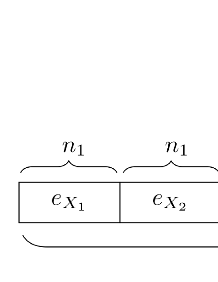
Suppose that there is an -error of length in the encoded codeword. We divide the error into sub-blocks , with each sub-block being of length (see Fig. 1). We then do the syndrome measurement for -errors by using the parity check matrix given in (40). The syndrome information can be derived by measuring the ancilla, which is given by
| (46) | |||||
where . We let which can be regarded as the logical error sequences in the outer code . Then we have
| (47) |
If the outer decoding can be conducted successfully, then the sequences are used as the inner syndrome information for .
The outer code must be decoded by mapping the syndrome information to the symbols over the extension field . Here we need a syndrome based decoding [9] of the outer code , which, if successful, will result in the exact inner syndrome sequence . The inner decoding follows using the dual of the inner code . In general, for any , we can always obtain a decoded error sequence such that by using some syndrome based decoder for , such as a syndrome table-look-up decoder. However, we do not need to do that and just let by assuming that is in a standard form, where “0” is a zero vector of length . Let be the decoded error sequence. There must be , where
| (48) |
is the generator matrix of . There are two cases: (1) which means that the decoded error is exactly the true error. (2) but they belong to the same coset of , which means that they are degenerate.
This phenomenon of degeneracy is quite different from the decoding of classical TPCs [52, 33, 35], where the decoding fails if the number of errors in one sub-block exceeds the error correction ability of the inner codes. As such, AQCTPCs can correct many more -errors than their classical TPC counterparts. If , whenever the error is separated into different sub-blocks in Fig. 1, the number of erroneous sub-blocks will be at most . This means that either the error will always be detectable or that the error is undetectable but harmless since it is degenerate. Thus the -distance is at least . Therefore we have an AQCTPC with the parameters . ∎
In the proof of Theorem III.1, we have given the decoding of AQCTPCs for correcting -errors. We summarize and provide the whole decoding process in Algorithm 1.
Divide into sub-blocks, each sub-block is of length .
Map to with elements over the extension field .
Do the outer decoding according to the syndrome information .
On the other hand, like the serial decoding of classical CCs, the decoding of -errors in AQCTPCs can also be done serially, i.e., an inner decoding followed by an outer decoding. However, the decoding algorithm for classical CCs can not be used to decode -errors directly. Instead, a modified version of syndrome-based decoding is needed, as explained next.
Before performing the decoding, the ancilla needs to be measured first to determine the syndrome information. Denote the encoded quantum basis states of the AQCTPC by
| (49) |
where . Suppose that a -error happens to the encoded sate (49), then
| (50) |
First we take the syndrome measurement using the inner parity check matrix to get the inner syndrome information
| (51) |
where and . The inner decodings are done first according to the inner syndrome information . They result in decoded error sequences , each of length . Denote by . We add the decoded result to (50), and then perform the measurement using the parity check matrix to get the outer syndrome information
| (52) | |||||
Discarding the zero part in due to the 0 sub-block in , the punctured is then mapped into a sequence with elements over field .
The outer decoding is done with a syndrome-based decoding of according to the outer syndrome information . If the outer decoding is successful, we can obtain a decoded sequence with elements over . Then we map the sequence back to the basis field , and derive a decoded error sequence with elements over , where is the sub-sequence of length . But notice that is incomplete due to the 0 sub-block in . In order to derive the fully-decoded error sequence, we only need to do some operations according to the inner syndrome information in (51). Denote by and , where denotes the unknown errors in and is of length . Suppose that , where is of size and is an invertible matrix, then we have and then , where .
Similar to classical CCs, no matter how many -errors happen in each sub-block of length , the outer decoding will not be affected provided that the total number of erroneous sub-blocks does not exceed the error correction ability of the outer code . A summary of the full decoding process is provided in Algorithm 2. A complexity analysis of the whole decoding process follows.
In terms of decoding -errors with the TPC, we first need to map the outer decoding sequence from to whose running time complexity is (see Algorithm 1, lines -). And it is easy to see that the complexity of the inner syndrome decoding of is since we just need to do , for . Therefore, the inner decoding complexity (IDC) of the TPC is . Recall that the IDC of classical TPCs is by using the maximum likelihood (ML) decoding in general, which is enormous if is large. Even though the inner codes can be efficiently decoded, see, e.g., [52, 34], the IDC of TPCs is still . Here, in quantum cases, we consider error degeneracy in the inner decoding and significantly reduce the IDC of TPCs to in general.
It is easy to see that the outer decoding complexity (ODC) of TPCs is completely determined by the outer constituent codes. Thus if the outer codes can be decoded efficiently, the whole decoding of TPCs is efficient. For example, we let the outer codes be the Reed-Solomon (RS) codes or the generalized Reed-Solomon (GRS) codes that satisfy the dual-containing relationship [64, 63]. They can be decoded efficiently in time polynomial to their block length, e.g., by using the Berlekamp-Massey (BM) algorithm, see [9, 10, 52]. Then the whole decoding of TPCs for correcting -errors can be done efficiently in polynomial time.
Do the outer decoding according to and .
When correcting -errors by using the CC, it is easy to see that the decoding complexity is the sum of the complexities of the inner and outer decodings. Thus, the CC is efficiently decodable provided that the constituent codes and can be decoded efficiently, e.g., in time polynomial to the block length [9, 10]. Overall, we can conclude that the entire AQCTPC decoding process for correcting both -errors and -errors is efficient provided that the inner and outer constituent codes are efficiently decodable.
Similar to the generalization of classical CCs and TPCs, we can generalize the concatenation scheme of AQCTPCs by combining GCCs with GTPCs. Let be -ary linear codes. Let and be -ary linear codes, respectively. Denote by linear codes obtained by partitioning the generator matrix of into submatrices. Then we have the following result about the dual-containing relationship between GCCs and GTPCs.
Lemma III.2
Let be the GTPC of and , and let be the GCC of and . If for all , then there is .
Proof:
We use the notations for GTPCs and GCCs given in Preliminaries. Denote the collection of duals matrix (cdm) (see Ref. [35]) of in (36) by
| (53) |
with , for , and . Then the parity check matrix of the GCC is given by
| (54) |
And the parity check matrix of the GTPC is given by
| (55) |
According to Ref. [35] and Ref. [45], we know the following two properties about the cdm of :
-
•
, for all , and .
-
•
is of full rank, for all .
Since is of full rank, we can always find an invertible matrix such that is an identity matrix, for . If , which means that for all , then there is and we have . ∎
Theorem III.2
There exist generalized AQCTPCs with parameters
| (56) |
where , .
Proof:
By combining Lemma II.1 and Lemma III.1, we can obtain the generalized AQCTPCs with parameters
| (57) |
We use the GCCs to correct -errors and thus the -distance of the generalized AQCTPC is given by . Next we need to compute the -distance of . Suppose that there is an -error of length in the encoded codeword. Denote
| (62) | |||||
by the syndrome information obtained by measuring the ancilla and let , . Suppose that for some , we have . Similar to the proof of Theorem III.1, if , then we must have and then the error can be detected or but the error is degenerate. Therefore we have . ∎
It should be noticed in the proof of Theorem III.2 that, we only give a minimum limit of the distance . In the practical error correction, e.g., in [50] for classical GCCs, we have syndrome information to be used for the decoding and then the generalized AQCTPCs can correct many more -errors beyond the minimum distance limit in Theorem III.2 in practice.
IV Families of AQCTPCs
In this section, we provide examples of AQCTPCs that outperform best-known AQCs in the literature. Since the inner constituent codes in AQCTPCs can be chosen arbitrarily, we can get varieties of AQCTPCs by using different types of the constituent codes. Although the construction of AQCTPCs is not restricted by the field size , in this section, we mainly focus on binary codes which may be more practical in the future application. For simplicity, if , we omit the subscript in the parameters of quantum and classical codes.
Firstly we use classical single-parity-check codes [9] as the inner constituent codes and we have the following result.
Corollary IV.1
There exists a family of binary AQCTPCs with parameters
| (63) |
where , , , , and are all integers.
Proof:
Let be a binary single-parity-check code with even codewords, and let and be two classical GRS codes. It is shown in [64] that if and , there exists . ∎
In Corollary IV.1, if we let , then we can also obtain a family of symmetric quantum codes with parameters
| (64) |
where , , . We first compare (64) with QBCH codes in [65]. It is known that the minimum distance of QBCH codes of length is upper bounded by ( is a constant). On the other hand, the minimum distance of our codes is upper bounded by which is larger than provided that .
For example, let , then the minimum distance of our codes can be as large as , which is almost linear to the length , while the dimension is larger than . If we let where is any constant, then the rate of our codes
| (65) |
is equal to as goes to infinity and . In [65], the rate of binary QBCH codes of CSS type is given by
| (66) |
where is the block length, is the multiplicative order of modulo , and . It is easy to see that is also asymptotic to as goes to infinity. However our codes have much better minimum distance upper bound than QBCH codes.
| AQCTPCs | Ref. [29] | AQCTPCs | Ref. [29] | AQCTPCs | Ref. [29] | |||
Then we compare AQCTPCs in Corollary IV.1 with the extension of asymmetric quantum MDS codes in [29]. For simplicity, we consider the extension of binary asymmetric QRS codes in [29] with parameters
| (67) |
where , , . In order to make a fair comparison between them, we let in Corollary IV.1 so that they have an equal or a similar block length. Let and , then it is easy to see that if , the dimension of AQCTPCs in (63) is larger than that of AQCs in (67). Further, AQCTPCs of length in Corollary IV.1 can be decoded efficiently in polynomial time and we have the following result.
Corollary IV.2
There exist AQCTPCs of length which can be decoded in arithmetic operations.
Proof:
First we consider the complexity of the decoding of -errors. The IDC of TPCs is according to the proof of Theorem III.1. It is known that GRS codes of length can be decoded in field operations by using the BM algorithm [9, 67]. Therefore the total decoding of TPCs requires arithmetic operations.
Then we consider the decoding of -errors by using the CC. If we use Algorithm 2 to do the decoding, we can only decode up to numbers of -errors. In order to decode any -error of weight smaller than half the minimum distance , we use the inner code to do the error detection for each sub-block of the CC. Suppose we can detect erroneous sub-blocks and suppose that there exist erroneous sub-blocks which are undetectable. As a result, there are erroneous positions which are known in the error sequence that corresponds to the outer code and, erroneous positions that are unknown. It is easy to see that if the weight of the -error is smaller than , we must have . Then we can decode the error sequence with errors in known locations and errors which are unknown by using the BM algorithm in arithmetic operations [9, 68]. Therefore the total complexity of decoding -errors is . Overall, the whole decoding of AQCTPCs of length can be fulfilled in arithmetic operations. ∎
In Table I, we make a comparison between parameters of AQCTPCs and the results in [29]. It is shown that AQCTPCs have a relatively large -distance and can have much better parameters than the codes in [29]. Further, the decoding complexity of AQCs in [29] of length is dominated by the RS code decoding whose complexity scales as by using the BM decoder, where . Then the decoding complexity of AQCs in [29] is . It is shown that both AQCTPCs in Corollary IV.2 and AQCs in [29] can be decoded efficiently in polynomial arithmetic operations. However, our codes have much better parameters than the codes in [29].
Next we use classical Simplex codes [9] that have a large minimum distance as the inner constituent codes. We show that Simplex codes can result in AQCTPCs with a large -distance .
Corollary IV.3
There exists a family of binary AQCTPCs with parameters
| (68) |
where , , , and .
Proof:
The proof proceeds in the same way as in Corollary IV.1 except we use classical Simplex codes as the inner constituent code. ∎
In particular, if we take and let and , where is a constant, then we have
| (69) |
where , , and . It is easy to see that as and can meet the quantum Gilbert-Varshamov (GV) bound for AQCs in [69]. Therefore we get a family of AQCTPCs with a very large -distance which is of approximately half the block length, at the same time, the dimension and the -distance can continue increasing as the block length goes to infinity. In Table II, we list several AQCTPCs with a large -distance which is of approximately half the block length. In particular, if , then the -distance of AQCTPCs in Corollary IV.3 could be larger than half the block length.
| AQCTPCs | AQCTPCs | ||||
|---|---|---|---|---|---|
In addition, if we use linear codes in [47] with best known parameters as the inner codes, we can get many new AQCTPCs with a relatively large -distance and very flexible code parameters. We list some of them in Table III. The -distances of the last four codes in Table III are much larger than half the block length, respectively. All the AQCTPCs in Table II and Table III have the largest -distance compared to existed AQCs with comparable block length and -distance .
| in Ref. [47] | in Theorem III.1 | AQCTPCs |
|---|---|---|
If we use asymptotically good linear codes that can attain the classical GV bound as the inner codes , we can get the following asymptotic result about AQCTPCs.
Corollary IV.4
There exists a family of -ary AQCTPCs with parameters
| (70) |
such that
| (71) | |||||
| (72) | |||||
| (73) |
where
| (74) |
is the -ary entropy function, , , and .
Proof:
On the other hand, besides using MDS codes as the outer constituent codes, we can also use AG codes that satisfy the dual-containing constraint [70, 44]. We will adopt the notation of AG codes used in [71, 44].
Theorem IV.1 ([44])
Let be an algebraic curve over of genus with at least rational points. For any , there exist two -ary AG codes and with such that , where and .
For , there is the following asymptotic result about asymmetric QAG codes in [44].
Theorem IV.2 ([44])
Let and let such that , then there exists a family of asymptotically good asymmetric QAG codes satisfying
| (76) |
By using similar code extension methods in [70] and the CSS construction of AQCs, one can obtain asymptotically good binary extensions of asymmetric QAG codes as follows.
Corollary IV.5
Let and let such that , then there exists a family of asymptotically good binary asymmetric QAG codes satisfying
| (77) |
Denote by a binary linear code and let be an algebraic curve over of genus with at least rational points. Then we have the following result for constructing AQCTPCs by using AG codes as outer codes.
Proposition IV.1
There exists a family of binary AQCTPCs with parameters
| (78) |
where , , , and . As goes to infinity, the following asymptotic bound of AQCTPCs holds
| (79) |
where , and are the relatively minimum distance of .
Proof:
According to Theorem IV.1, we know that there exist two -ary AG codes and such that , where and . Then from Theorem III.1, we can construct a family of binary AQCTPCs with parameters , where and . Denote by and the relatively minimum distance of , i.e., and . The asymptotic result can be obtained by Theorem IV.2. ∎
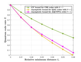
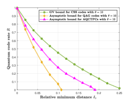
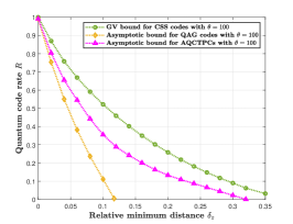
In Fig. , we compare the asymptotic bound of AQCTPCs in (79) with that of asymmetric QAG codes in (77). We also give the GV bound of CSS codes for comparisons. In order to get as good as possible asymptotic curves for AQCTPCs, we use different inner constituent codes to generate several piecewise asymptotic curves and then joint them together. In Fig. (a), we can see that the asymptotic bound of AQCTPCs is better than that for asymmetric QAG codes when the relative minimum distance . As the the asymmetry grows, it is shown in Fig. (b) and Fig. (c) that AQCTPCs perform much better than asymmetric QAG codes.
V Conclusions and Discussions
In this paper, we proposed the construction of asymmetric quantum concatenated and tensor product codes that combine the classical CCs and TPCs. The CCs correct the -errors and the TPCs correct the -errors. Compared to concatenation schemes like CQCs and QTPCs, the AQCTPC construction only requires that the outer constituent codes satisfy the dual-containing constraint; the inner constituent codes can be chosen freely. Further, AQCTPCs are highly degenerate codes and, as a result, they passively correct many -errors. To avoid issues with decoding, we present efficient syndrome-based decoding algorithms and show that if the inner and outer constituent codes are efficiently decodable, then the AQCTPC is also efficiently decodable. Particularly, the inner decoding complexity of TPCs is significantly reduced to in general. Further, we generalized the AQCTPC concatenation scheme by using GCCs and GTPCs.
To showcase the power of the method, we constructed many state-of-the-art AQCs. Through these constructions, we demonstrate how AQCTPCs can be superior to QBCH codes or asymmetric QAG codes as the block length goes to infinity; how they can have better parameters than the binary extension of asymmetric QRS codes; and how varieties of AQCTPCs with a large -distance can be designed by using some best known linear codes in [47]. In particular, we constructed a family of AQCTPCs with a -distance of approximately half the block length, and meanwhile with dimension and -distance that continue to increase as the block length goes to infinity. If , we obtain the first family of binary AQCs with the -distance larger than half the block length.
Our codes are practical to quantum communication channels with a large asymmetry and may be used in fault-tolerant quantum computation to deal with highly biased noise. In the next work, we may consider the construction and decoding of AQCTPCs by using some other constituent codes, e.g., the Polar codes.
Acknowledgment
The authors would like to thank the Editor and the referees for their valuable comments that are helpful to improve the presentation of their article. J. Fan thanks Prof. Yonghui Li and Prof. Martin Bossert for some earlier communications about tensor product codes.
References
- [1] L. Ioffe and M. Mézard, “Asymmetric quantum error-correcting codes,” Phys. Rev. A, vol. 75, p. 032345, 2007.
- [2] D. K. Tuckett, S. D. Bartlett, and S. T. Flammia, “Ultrahigh error threshold for surface codes with biased noise,” Phys. Rev. Lett., vol. 120, no. 5, p. 050505, 2018.
- [3] H. Häffner, C. F. Roos, and R. Blatt, “Quantum computing with trapped ions,” Phys. Rep., vol. 469, no. 4, pp. 155–203, 2008.
- [4] H. O. H. Churchill, F. Kuemmeth, J. W. Harlow, A. J. Bestwick, E. I. Rashba, K. Flensberg, C. H. Stwertka, T. Taychatanapat, S. K. Watson, and C. M. Marcus, “Relaxation and dephasing in a two-electron nanotube double quantum dot,” Phys. Rev. Lett., vol. 102, no. 16, p. 166802, 2009.
- [5] A. M. Steane, “Simple quantum error-correcting codes,” Phys. Rev. A, vol. 54, no. 6, p. 4741, 1996.
- [6] P. Aliferis and J. Preskill, “Fault-tolerant quantum computation against biased noise,” Phys. Rev. A, vol. 78, p. 052331, 2008.
- [7] P. K. Sarvepalli, A. Klappenecker, and M. Rötteler, “Asymmetric quantum codes: constructions, bounds and performance,” in Proc. Roy. Soc. A, vol. 465, 2009, pp. 1645–1672.
- [8] P. Brooks and J. Preskill, “Fault-tolerant quantum computation with asymmetric Bacon-Shor codes,” Phys. Rev. A, vol. 87, no. 3, p. 032310, 2013.
- [9] F. J. MacWilliams and N. J. A. Sloane, The Theory of Error-Correcting Codes. Amsterdam: The Netherlands: North-Holland, 1981.
- [10] S. Lin and D. J. Costello, Error Control Coding: Fundamentals and Applications, 2nd ed. Upper Saddle River, NJ: Prentice-Hall, Inc., 2004.
- [11] M. H. Azmi, J. Li, J. Yuan, and R. Malaney, “LDPC codes for soft decode-and-forward in half-duplex relay channels,” IEEE J. Sel. Areas Commun., vol. 31, no. 8, pp. 1402–1413, 2013.
- [12] J. Li, W. Chen, Z. Lin, and B. Vucetic, “Design of physical layer network coded LDPC code for a multiple-access relaying system,” IEEE Commun. Lett., vol. 17, no. 4, pp. 749–752, 2013.
- [13] Y. Yu, W. Chen, J. Li, X. Ma, and B. Bai, “Generalized binary representation for the nonbinary LDPC code with decoder design,” IEEE Trans. Commun., vol. 62, no. 9, pp. 3070–3083, 2014.
- [14] J. Li, J. Yuan, R. Malaney, M. H. Azmi, and M. Xiao, “Network coded LDPC code design for a multi-source relaying system,” IEEE Trans. Wirel. Commun., vol. 10, no. 5, pp. 1538–1551, 2011.
- [15] C. Galindo, F. Hernando, R. Matsumoto, and D. Ruano, “Asymmetric entanglement-assisted quantum error-correcting codes and BCH codes,” IEEE Access, vol. 8, pp. 18 571–18 579, 2020.
- [16] T. Brun, I. Devetak, and M.-H. Hsieh, “Correcting quantum errors with entanglement,” Science, vol. 314, no. 5798, pp. 436–439, 2006.
- [17] M.-H. Hsieh, W.-T. Yen, and L.-Y. Hsu, “High performance entanglement-assisted quantum LDPC codes need little entanglement,” IEEE Trans. Inf. Theory, vol. 57, no. 3, pp. 1761–1769, 2011.
- [18] M. M. Wilde, M.-H. Hsieh, and Z. Babar, “Entanglement-assisted quantum Turbo codes,” IEEE Trans. Inf. Theory, vol. 60, no. 2, pp. 1203–1222, 2013.
- [19] M.-H. Hsieh and M. M. Wilde, “Entanglement-assisted communication of classical and quantum information,” IEEE Trans. Inf. Theory, vol. 56, no. 9, pp. 4682–4704, 2010.
- [20] M.-H. Hsieh, T. A. Brun, and I. Devetak, “Entanglement-assisted quantum quasicyclic low-density parity-check codes,” Phys. Rev. A, vol. 79, no. 3, p. 032340, 2009.
- [21] J. Fan, H. Chen, and J. Xu, “Constructions of -ary entanglement-assisted quantum MDS codes with minimum distance greater than + 1,” Quantum Inf. Comput., vol. 16, no. 5-6, pp. 423–434, 2016.
- [22] D. K. Tuckett, S. D. Bartlett, S. T. Flammia, and B. J. Brown, “Fault-tolerant thresholds for the surface code in excess of 5 under biased noise,” Phys. Rev. Lett., vol. 124, p. 130501, 2020.
- [23] D. K. Tuckett, A. S. Darmawan, C. T. Chubb, S. Bravyi, S. D. Bartlett, and S. T. Flammia, “Tailoring surface codes for highly biased noise,” Phys. Rev. X, vol. 9, no. 4, p. 041031, 2019.
- [24] J. P. Bonilla-Ataides, D. K. Tuckett, S. D. Bartlett, S. T. Flammia, and B. J. Brown, “The XZZX surface code,” arXiv:2009.07851, 2020.
- [25] S. A. Aly, “Asymmetric quantum BCH codes,” in Proc. IEEE Int. Conf. Comput. Eng. System, Cairo, Egypt, Nov. 2008, pp. 157–162.
- [26] R. Li, G. Xu, and L. Guo, “On two problems of asymmetric quantum codes,” Int. J. Mod. Phys. B, vol. 28, no. 06, p. 1450017, 2014.
- [27] M. F. Ezerman, S. Jitman, S. Ling, and D. V. Pasechnik, “CSS-like constructions of asymmetric quantum codes,” IEEE Trans. Inf. Theory, vol. 59, no. 10, pp. 6732–6754, 2013.
- [28] J. Cannon, W. Bosma, C. Fieker, and A. Steel, Handbook of Magma Functions, Sydney, 2008. [Online]. Available: https://magma.maths.usyd.edu.au/magma/handbook/
- [29] G. G. La Guardia, “Asymmetric quantum Reed-Solomon and generalized Reed-Solomon codes,” Quantum Inf. Process., vol. 11, no. 2, pp. 591–604, 2012.
- [30] C. Galindo, O. Geil, F. Hernando, and D. Ruano, “Improved constructions of nested code pairs,” IEEE Trans. Inf. Theory, vol. 64, no. 4, pp. 2444–2459, 2017.
- [31] G. G. La Guardia, “On the construction of asymmetric quantum codes,” Int. J. Theor. Phys., vol. 53, no. 7, pp. 2312–2322, 2014.
- [32] G. D. Forney Jr, “Concatenated codes.” Ph.D. dissertation, Massachusetts Institute of Technology, 1965.
- [33] J. K. Wolf, “On codes derivable from the tensor product of check matrices,” IEEE Trans. Inf. Theory, vol. 11, no. 2, pp. 281–284, 1965.
- [34] ——, “An introduction to tensor product codes and applications to digital storage systems,” in Proc. IEEE ITW, Chengdu, China, Oct. 2006, pp. 6–10.
- [35] J. Maucher, V. V. Zyablov, and M. Bossert, “On the equivalence of generalized concatenated codes and generalized error location codes,” IEEE Trans. Inf. Theory, vol. 46, no. 2, pp. 642–649, 2000.
- [36] E. Knill and R. Laflamme, “Concatenated quantum codes,” arXiv preprint quant-ph/9608012, 1996.
- [37] D. Gottesman, “Stabilizer codes and quantum error correction,” Ph.D. dissertation, California Institute of Technology, 1997.
- [38] M. Grassl and M. Rötteler, “Quantum block and convolutional codes from self-orthogonal product codes,” in Proc. IEEE Int. Symp. Inf. Theory, Adelaide, SA, Australia, Sept. 2005, pp. 1018–1022.
- [39] J. Fan, Y. Li, M.-H. Hsieh, and H. Chen, “On quantum tensor product codes,” Quantum Inf. Comput., vol. 17, no. 1314, pp. 1105–1122, 2017.
- [40] G. G. La Guardia, “Asymmetric quantum product codes,” Int. J. Quantum Inf., vol. 10, no. 01, p. 1250005, 2012.
- [41] P. J. Nadkarni and S. S. Garani, “Entanglement assisted binary quantum tensor product codes,” in Proc. IEEE ITW. Kaohsiung, Taiwan: IEEE, Nov. 2017, pp. 219–223.
- [42] M.-H. Hsieh and F. Le Gall, “NP-hardness of decoding quantum error-correction codes,” Phys. Rev. A, vol. 83, no. 5, p. 052331, 2011.
- [43] A. R. Calderbank and P. W. Shor, “Good quantum error-correcting codes exist,” Phys. Rev. A, vol. 54, no. 2, p. 1098, 1996.
- [44] L. Wang, K. Feng, S. Ling, and C. Xing, “Asymmetric quantum codes: characterization and constructions,” IEEE Trans. Inf. Theory, vol. 56, no. 6, pp. 2938–2945, 2010.
- [45] J. Fan and H. Chen, “Comments on and Corrections to “On the equivalence of generalized concatenated codes and generalized error location codes”,” IEEE Trans. Inf. Theory, vol. 63, no. 8, pp. 5437–5439, 2017.
- [46] H. Imai and H. Fujiya, “Generalized tensor product codes,” IEEE Trans. Inf. Theory, vol. 27, no. 2, pp. 181–187, 1981.
- [47] M. Grassl, “Bounds on the minimum distance of linear codes and quantum codes,” Online available at http://www.codetables.de, 2007.
- [48] D. J. Costello and G. D. Forney, “Channel coding: The road to channel capacity,” Proc. IEEE, vol. 95, no. 6, pp. 1150–1177, 2007.
- [49] I. Zhilin, P. Rybin, and V. Zyablov, “High-rate codes for high-reliability data transmission,” in Proc. IEEE Int. Symp. Inf. Theory. Hong Kong, China: IEEE, Jun. 2015, pp. 256–260.
- [50] J. Spinner, J. Freudenberger, and S. Shavgulidze, “A soft input decoding algorithm for generalized concatenated codes,” IEEE Trans. Commun., vol. 64, no. 9, pp. 3585–3595, 2016.
- [51] M. Rajab, S. Shavgulidze, and J. Freudenberger, “Soft-input bit-flipping decoding of generalised concatenated codes for application in non-volatile Flash memories,” IET Commun., vol. 13, no. 4, pp. 460–467, 2018.
- [52] H. Alhussien and J. Moon, “An iteratively decodable tensor product code with application to data storage,” IEEE J. Sel. Areas Commun., vol. 2, no. 28, pp. 228–240, 2010.
- [53] P. Chaichanavong and P. H. Siegel, “Tensor-product parity code for magnetic recording,” IEEE Trans. Magn., vol. 42, no. 2, pp. 350–352, 2006.
- [54] ——, “Tensor-product parity codes: Combination with constrained codes and application to perpendicular recording,” IEEE Trans. Magn., vol. 42, no. 2, pp. 214–219, 2006.
- [55] A. Fahrner, H. Griesser, R. Klarer, and V. V. Zyablov, “Low-complexity GEL codes for digital magnetic storage systems,” IEEE Trans. Magn., vol. 40, no. 4, pp. 3093–3095, 2004.
- [56] R. Gabrys, E. Yaakobi, and L. Dolecek, “Graded bit-error-correcting codes with applications to Flash memory,” IEEE Trans. Inf. Theory, vol. 59, no. 4, pp. 2315–2327, 2013.
- [57] M. N. Kaynak, P. R. Khayat, and S. Parthasarathy, “Classification codes for soft information generation from hard Flash reads,” IEEE J. Sel. Areas Commun., vol. 32, no. 5, pp. 892–899, 2014.
- [58] P. Huang, E. Yaakobi, H. Uchikawa, and P. H. Siegel, “Linear locally repairable codes with availability,” in Proc. IEEE Int. Symp. Inf. Theory, Hong Kong, China, Jun. 2015, pp. 1871–1875.
- [59] ——, “Binary linear locally repairable codes,” arXiv preprint arXiv:1511.06960, 2015.
- [60] M. Blaum, “Extended integrated interleaved codes over any field with applications to locally recoverable codes,” IEEE Trans. Inf. Theory, vol. 66, no. 2, pp. 936–956, 2019.
- [61] P. Trifonov, V. Miloslavskaya, C. Chen, and Y. Wang, “Fast encoding of polar codes with Reed-Solomon kernel,” IEEE Trans. Commun., vol. 64, no. 7, pp. 2746–2753, 2016.
- [62] M. Grassl, W. Geiselmann, and T. Beth, “Quantum Reed-Solomon codes,” in Applied Algebra, Algebraic Algorithms and Error-correcting Codes. Springer, 1999, pp. 231–244.
- [63] M. Grassl, T. Beth, and M. Rötteler, “On optimal quantum codes,” Int. J. Quant. Inf., vol. 2, no. 01, pp. 55–64, 2004.
- [64] M. F. Ezerman, S. Jitman, H. M. Kiah, and S. Ling, “Pure asymmetric quantum MDS codes from CSS construction: A complete characterization,” Int. J. Quantum Inf., vol. 11, no. 03, p. 1350027, 2013.
- [65] S. A. Aly, A. Klappenecker, and P. K. Sarvepalli, “On quantum and classical BCH codes,” IEEE Trans. Inf. Theory, vol. 53, no. 3, pp. 1183–1188, 2007.
- [66] A. R. Calderbank, E. M. Rains, P. Shor, and N. J. Sloane, “Quantum error correction via codes over GF(4),” IEEE Trans. Inf. Theory, vol. 44, no. 4, pp. 1369–1387, 1998.
- [67] D. V. Sarwate, “On the complexity of decoding Goppa codes (Corresp.),” IEEE Transactions on Information Theory, vol. 23, no. 4, pp. 515–516, 1977.
- [68] G. Forney, “Generalized minimum distance decoding,” IEEE Transactions on Information Theory, vol. 12, no. 2, pp. 125–131, 1966.
- [69] R. Matsumoto, “Two Gilbert-Varshamov-type existential bounds for asymmetric quantum error-correcting codes,” Quantum Inf. Process., vol. 16, no. 12, p. 285, 2017.
- [70] A. Ashikhmin, S. Litsyn, and M. A. Tsfasman, “Asymptotically good quantum codes,” Phys. Rev. A, vol. 63, no. 3, p. 032311, 2001.
- [71] M. Tsfasman and S. Vlăduţ, Algebraic-Geometric Codes. Dordrecht: Kluwer, 1991.