Asymmetric Totally-corrective Boosting for Real-time Object Detection
Abstract
Real-time object detection is one of the core problems in computer vision. The cascade boosting framework proposed by Viola and Jones has become the standard for this problem. In this framework, the learning goal for each node is asymmetric, which is required to achieve a high detection rate and a moderate false positive rate. We develop new boosting algorithms to address this asymmetric learning problem. We show that our methods explicitly optimize asymmetric loss objectives in a totally corrective fashion. The methods are totally corrective in the sense that the coefficients of all selected weak classifiers are updated at each iteration. In contract, conventional boosting like AdaBoost is stage-wise in that only the current weak classifier’s coefficient is updated. At the heart of the totally corrective boosting is the column generation technique. Experiments on face detection show that our methods outperform the state-of-the-art asymmetric boosting methods.
1 Introduction
Due to its important applications in video surveillance, interactive human-machine interface etc, real-time object detection has attracted extensive research recently [1, 2, 3, 4, 5, 6]. Although it was introduced a decade ago, the boosted cascade classifier framework of Viola and Jones [2] is still considered as the most promising approach for object detection, and this framework is the basis which many papers have extended.
One difficulty in object detection is the problem is highly asymmetric. A common method to detect objects in an image is to exhaustively search all sub-windows at all possible scales and positions in the image, and use a trained model to detect target objects. Typically, there are only a few targets in millions of searched sub-windows. The cascade classifier framework partially solves the asymmetry problem by splitting the detection process into several nodes. Only those sub-windows passing through all nodes are classified as true targets. At each node, we want to train a classifier with a very high detection rate (e.g., ) and a moderate false positive rate (e.g., around ). The learning goal of each node should be asymmetric in order to achieve optimal detection performance. A drawback of standard boosting like AdaBoost in the context of the cascade framework is it is designed to minimize the overall false rate. The losses are equal for misclassifying a positive example and a negative example, which makes it not be able to build an optimal classifier for the asymmetric learning goal.
Many subsequent works attempt to improve the performance of object detectors by introducing asymmetric loss functions to boosting algorithms. Viola and Jones proposed asymmetric AdaBoost [3], which applies an asymmetric multiplier to one of the classes. However, this asymmetry is absorbed immediately by the first weak classifier because AdaBoost’s optimization strategy is greedy. In practice, they manually apply the -th root of the multiplier on each iteration to keep the asymmetric effect throughout the entire training process. Here is the number of weak classifiers. This heuristic cannot guarantee the solution to be optimal and the number of weak classifiers need to be specified before training. AdaCost presented by Fan et al. [7] adds a cost adjustment function on the weight updating strategy of AdaBoost. They also pointed out that the weight updating rule should consider the cost not only on the initial weights but also at each iteration. Li and Zhang [8] proposed FloatBoost to reduce the redundancy of greedy search by incorporating floating search with AdaBoost. In FloatBoost, the poor weak classifiers are deleted when adding the new weak classifier. Xiao et al. [9] improved the backtrack technique in [8] and exploited the historical information of preceding nodes into successive node learning. Hou et al. [10] used varying asymmetric factors for training different weak classifiers. However, because the asymmetric factor changes during training, the loss function remains unclear. Pham et al. [11] presented a method which trains the asymmetric AdaBoost [3] classifiers under a new cascade structure, namely multi-exit cascade. Like soft cascade [12], boosting chain [9] and dynamic cascade [13], multi-exit cascade is a cascade structure which takes the historical information into consideration. In multi-exit cascade, the -th node “inherits” weak classifiers selected at the preceding nodes. Wu et al. [14] stated that feature selection and ensemble classifier learning can be decoupled. They designed a linear asymmetric classifier (LAC) to adjust the linear coefficients of the selected weak classifiers. Kullback-Leibler Boosting [15] iteratively learns robust linear features by maximizing the Kullback-Leibler divergence.
Much of the previous work is based on AdaBoost and achieves the asymmetric learning goal by heuristic weights manipulations or post-processing techniques. It is not trivial to assess how these heuristics affect the original loss function of AdaBoost. In this work, we construct new boosting algorithms directly from asymmetric losses. The optimization process is implemented by column generation. Experiments on toy data and real data show that our algorithms indeed achieve the asymmetric learning goal without any heuristic manipulation, and can outperform previous methods.
Therefore, the main contributions of this work are as follows.
-
1.
We utilize a general and systematic framework (column generation) to construct new asymmetric boosting algorithms, which can be applied to a variety of asymmetric losses. There is no heuristic strategy in our algorithms which may cause suboptimal solutions. In contrast, the global optimal solution is guaranteed for our algorithms.
Unlike Viola-Jones’ asymmetric AdaBoost [3], the asymmetric effect of our methods spreads over the entire training process. The coefficients of all weak classifiers are updated at each iteration, which prevents the first weak classifier from absorbing the asymmetry. The number of weak classifiers does not need to be specified before training.
-
2.
The asymmetric totally-corrective boosting algorithms introduce the asymmetric learning goal into both feature selection and ensemble classifier learning. Both the example weights and the linear classifier coefficients are learned in an asymmetric way.
-
3.
In practice, L-BFGS-B [16] is used to solve the primal problem, which runs much faster than solving the dual problem and also less memory is needed.
-
4.
We demonstrate that with the totally corrective optimization, the linear coefficients of some weak classifiers are set to zero by the algorithm such that fewer weak classifiers are needed. We present analysis on the theoretical condition and show how useful the historical information is for the training of successive nodes.
2 Asymmetric losses
In this section, we propose two asymmetric losses, which are motivated by asymmetric AdaBoost [3] and cost-sensitive LogitBoost [17], respectively.
We first introduce an asymmetric cost in the following form:
| (4) |
Here is the input data, is the label and is the learned classifier. Viola and Jones [3] directly take the product of and the exponential loss as the asymmetric loss:
where is the indicator function. In a similar manner, we can also form an asymmetric loss from the logistic loss :
| (5) |
where is the logistic loss function.
Masnadi-Shirazi and Vasconcelos [17] proposed cost-sensitive boosting algorithms which optimize different versions of cost-sensitive losses by the means of gradient descent. They proved that the optimal cost-sensitive predictor minimizes the expected loss:
With fixing to , the expected loss can be reformulated to
| (6) |
3 Asymmetric totally-corrective boosting
In this section, we construct asymmetric totally-corrective boosting algorithms (termed AsymBoostTC here) from the losses (5) and (6) discussed previously. In contrast to the methods constructing boosting-like algorithms in [17], [18] and [19], we use column generation to design our totally corrective boosting algorithms, inspired by [20] and [5].
Suppose there are training examples ( positives and negatives), and the sequence of examples are arranged according to the labels (positives first). The pool contains available weak classifiers. The matrix contains binary outputs of weak classifiers in for training examples, namely . We are aiming to learn a linear combination . and are costs for misclassifying positives and negatives, respectively. We assign the asymmetric factor and restrict to , thus and are fixed for a given .
The problems of the two AsymBoostTC algorithms can be expressed as:
| (7) |
where , and
| (8) |
where . In both (7) and (8), stands for the margin of the -th training example. We refer (7) as AsymBoostTC1 and (8) as AsymBoostTC2. Note that here the optimization problems are -norm regularized. It is possible to use other format of regularization such as the -norm.
First we introduce a fact that the Fenchel conjugate [21] of the logistic loss function is
Now we derive the Lagrange dual [21] of AsymBoostTC1. The Lagrangian of (7) is
The dual function
The dual problem is
| (9) |
Since the problem (7) is convex and the Slater’s conditions are satisfied [21], the duality gap between the primal (7) and the dual (3) is zero. Therefore, the solutions of (7) and (3) are the same. Through the KKT condition, the gradient of Lagrangian (3) over primal variable and dual variable should vanish at the optimum. Therefore, we can obtain the relationship between the optimal value of and :
| (10) |
Similarly, we can get the dual problem of AsymBoostTC2, which is expressed as:
| (11) |
with
| (12) |
In practice, the total number of weak classifiers, , could be extremely large, so we can not solve the primal problems (7) and (8) directly. However equivalently, we can optimize the duals (3) and (3) iteratively using column generation [20]. In each round, we add the most violated constraint by finding a weak classifier satisfying:
| (13) |
This step is the same as training a weak classifier in AdaBoost and LPBoost, in which one tries to find a weak classifier with the maximal edge (i.e. the minimal weighted error). The edge of is defined as , which is the inverse of the weighted error. Then we solve the restricted dual problem with one more constraint than the previous round, and update the linear coefficients of weak classifiers () and the weights of training examples (). Adding one constraint into the dual problem corresponds to adding one variable into the primal problem. Since the primal problem and dual problem are equivalent, we can either solve the restricted dual or the restricted primal in practice. The algorithms of AsymBoostTC1 and AsymBoostTC2 are summarized in Algorithm 1. Note that, in practice, in order to achieve specific false negative rate (FNR) or false positive rate (FPR), an offset is needed to be added into the final strong classifier: , which can be obtained by a simple line search. The new weak classifier corresponds to an extra variable to the primal and an extra constraint to the dual. Thus, the minimal value of the primal decreases with growing variables, and the maximal value of the dual problem also decreases with growing constraints. Furthermore, as the optimization problems involved are convex, Algorithm 1 is guaranteed to converge to the global optimum.
Next we show how AsymBoostTC introduces the asymmetric learning into feature selection and ensemble classifier learning. Decision stumps are the most commonly used type of weak classifiers, and each stump only uses one dimension of the features. So the process of training weak classifiers (decision stumps) is equivalent to feature selection. In our framework, the weak classifier with the maximum edge (i.e. the minimal weighted error) is selected. From (10) and (12), the weight of -th example, namely , is affected by two factors: the asymmetric factor and the current margin . If we set , the weighting strategy goes back to being symmetric. On the other hand, the coefficients of the linear classifier, namely , are updated by solving the restricted primal problem at each iteration. The asymmetric factor in the primal is absorbed by all the weak classifiers currently learned. So feature selection and ensemble classifier learning both consider the asymmetric factor .
if and , then break;
5
5
5
5
5
The number of variables of the primal problem is the number of weak classifiers, while for the dual problem, it is the number of training examples. In the cascade classifiers for face detection, the number of weak classifiers is usually much smaller than the number of training examples, so solving the primal is much cheaper than solving the dual. Since the primal problem has only simple box-bounding constraints, we can employ L-BFGS-B [16] to solve it. L-BFGS-B is a tool based on the quasi-Newton method for bound-constrained optimization.
Instead of maintaining the Hessian matrix, L-BFGS-B only needs the recent several updates of values and gradients for the cost function to approximate the Hessian matrix. Thus, L-BFGS-B requires less memory when running. In column generation, we can use the results from previous iteration as the starting point of current problem, which leads to further reductions in computation time.
The complementary slackness condition [21] suggests that . So we can get the conditions of sparseness:
| (14) |
This means that, if the weak classifier is so “weak” that its edge is less than under the current distribution , its contribution to the ensemble classifier is “zero”. From another viewpoint, the -norm regularization term in the primal (7) and (8), leads to a sparse result. The parameter controls the degree of the sparseness. The larger is, the sparser the result would be.
4 Experiments
4.1 Results on synthetic data
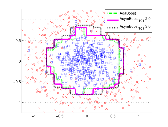
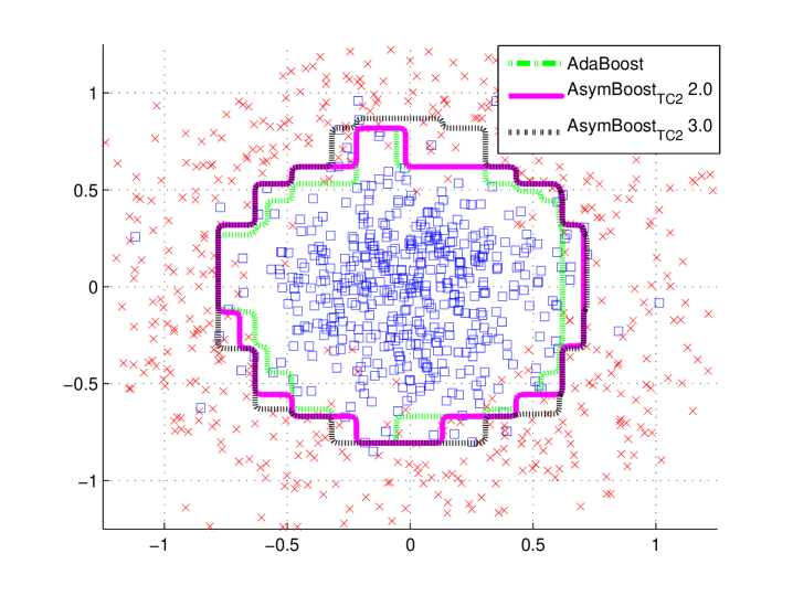
To show the behavior of our algorithms, we construct a D data set, in which the positive data follow the D normal distribution (), and the negative data form a ring with uniformly distributed angles and normally distributed radius (). Totally examples are generated ( positives and negatives), of data for training and the other half for test. We compare AdaBoost, AsymBoostTC1 and AsymBoostTC2 on this data set. All the training processes are stopped at decision stumps. For AsymBoostTC1 and AsymBoostTC2, we fix to , and use a group of ’s .
From Figures 1 and , we find that the larger is, the bigger the area for positive output becomes, which means that the asymmetric LogitBoost tends to make a positive decision for the region where positive and negative data are mixed together. Another observation is that AsymBoostTC1 and AsymBoostTC2 have almost the same decision boundaries on this data set with same ’s.
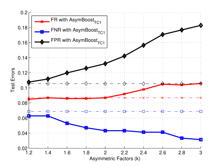
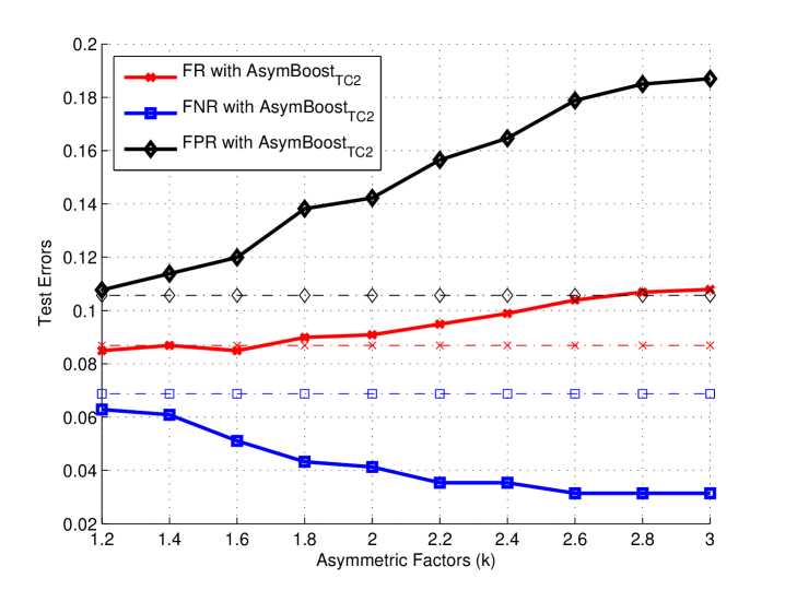
Figures 1 and demonstrate trends of false rates with the growth of asymmetric factor (). The results of AdaBoost is considered as the baseline. For all ’s, AsymBoostTC1 and AsymBoostTC2 achieve lower false negative rates and higher false positive rates than AdaBoost. With the growth of , AsymBoostTC1 and AsymBoostTC2 become more aggressive to reduce the false negative rate, with the sacrifice of a higher false positive rate.
4.2 Face detection
We collect mirrored frontal face images and about large background images. face images and background images are used for training, and face images and background images for validation. Five basic types of Haar features are calculated on each image, and totally generate features. Decision stumps on those features construct the pool of weak classifiers.
Single-node detectors Single-node classifiers with AdaBoost, AsymBoostTC1 and AsymBoostTC2 are trained. The parameters and are simply set to and . faces and non-faces are used for training, while faces and non-faces are used for test. The training/validation non-faces are randomly cropped from training/validation background images.
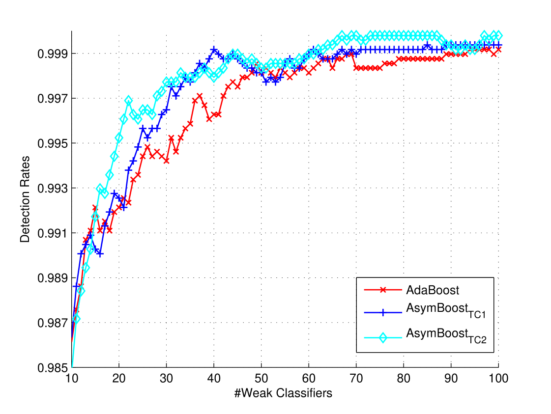
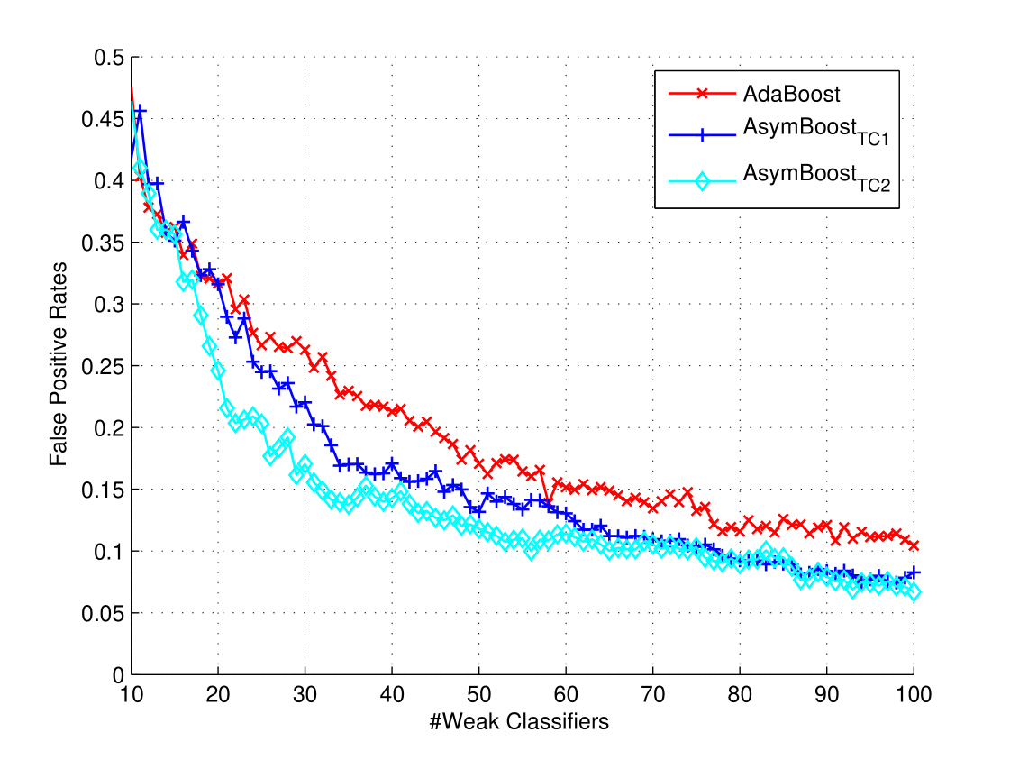
Figure 2 shows curves of detection rate with the false positive rate fixed at , while curves of false positive rates with detection rate are shown in Figure 2 . We set the false positive rate fixed to rather than the commonly used in order to slow down the increasing speed of detection rates, otherwise detection rates would converge to immediately. The increasing/decreasing speed of detection rate/false positive rate is faster than reported in [8] and [9]. The reason is possibly that we use examples for training and for testing, which are smaller than the data used in [8] and [9] ( training examples and test examples). We can see that under both situations, our algorithms achieve better performances than AdaBoost in most cases.
The benefits of our algorithms can be expressed in two-fold: (1) Given the same learning goal, our algorithms tend to use smaller number of weak classifiers. For example, from Figure 2 , if we want a classifier with a detection rate and a false positive rate, AdaBoost needs at least weak classifiers while AsymBoostTC1 needs and AsymBoostTC2 needs only . (2) Using the same number of weak classifiers, our algorithms achieve a higher detection rate or a lower false positive rate. For example, from Figure 2 , using weak classifiers, both AsymBoostTC1 and AsymBoostTC2 achieve higher detection rates ( and ) than AdaBoost ().
Complete detectors Secondly, we train complete face detectors with AdaBoost, asymmetric-AdaBoost, AsymBoostTC1 and AsymBoostTC2. All detectors are trained using the same training set. We use two types of cascade framework for the detector training: the traditional cascade of Viola and Jones [2] and the multi-exit cascade presented in [11]. The latter utilizes decision information of previous nodes when judging instances in the current node. For fair comparison, all detectors use nodes and weak classifiers. For each node, faces + non-faces are used for training, and faces + non-faces are used for validation. All non-faces are cropped from background images. The asymmetric factor for asymmetric-AdaBoost, AsymBoostTC1 and AsymBoostTC2 are selected from . The regularization factor for AsymBoostTC1 and AsymBoostTC2 are chosen from . It takes about four hours to train a AsymBoostTC face detector on a machine with Intel Xeon E5520 cores and GB memory. Comparing with AdaBoost, only around hour extra time is spent on solving the primal problem at each iteration. We can say that, in the context of face detection, the training time of AsymBoostTC is nearly the same as AdaBoost.
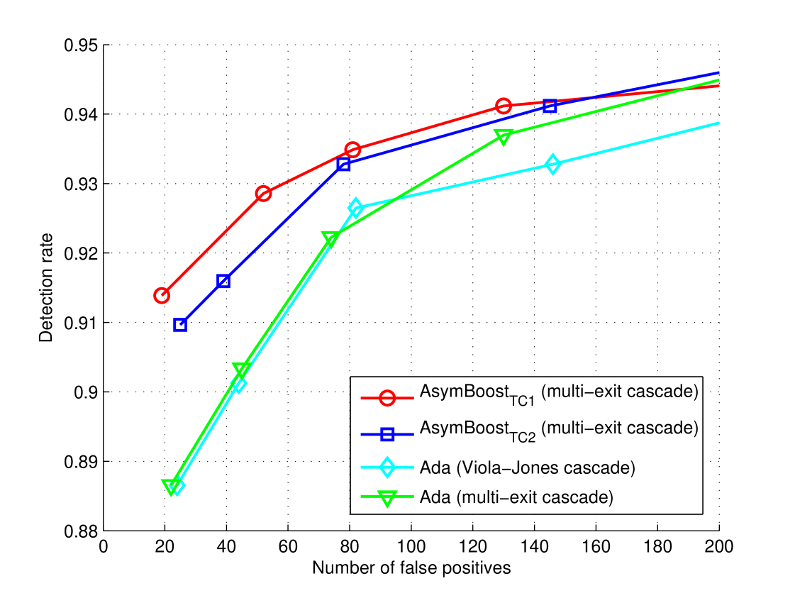
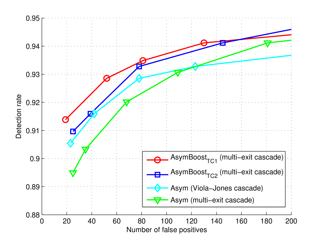
ROC curves on the CMU/MIT data set are shown in Figure 3. Those images containing ambiguous faces are removed and images are retained. From the figure, we can see that, asymmetric-AdaBoost outperforms AdaBoost in both Viola-Jones cascade and multi-exit cascade, which coincide with what reported in [3]. Our algorithms have better performances than all other methods in all points and the improvements are more significant when the false positives are less than , which is the most commonly used region in practice.
As mentioned in the previous section, our algorithms produce sparse results to some extent. Some linear coefficients are zero when the corresponding weak classifiers satisfy the condition (14). In the multi-exit cascade, the sparse phenomenon becomes more clear. Since correctly classified negative data are discarded after each node is trained, the training data for each node are different. The “closer” nodes share more common training examples, while the nodes “far away” from each other have distinct training data. The greater the distance between two nodes, the more uncorrelated they become. Therefore, the weak classifiers in the early nodes may perform poorly on the last node, thus tending to obtain zero coefficients. We call those weak classifiers with non-zero coefficients “effective” weak classifiers. Table 1 shows the ratios of “effective” weak classifiers contributed by one node to a specific successive node. To save space, only the first nodes are demonstrated. We can see that, the ratio decreases with the growth of the node index, which means that the farther the preceding node is from the current node, the less useful it is for the current node. For example, the first node has almost no contribution after the eighth node. Table 2 shows the number of effective weak classifiers used by our algorithm and the traditional stage-wise boosting. All weak classifiers in stage-wise boosting have non-zero coefficients, while our totally-corrective algorithm uses much less effective weak classifiers.
| Node Index | 1 | 2 | 3 | 4 | 5 | 6 | 7 | 8 | 9 | 10 | 11 | 12 | 13 | 14 | 15 |
|---|---|---|---|---|---|---|---|---|---|---|---|---|---|---|---|
| 1 | |||||||||||||||
| 2 | |||||||||||||||
| 3 | |||||||||||||||
| 4 | |||||||||||||||
| 5 | |||||||||||||||
| 6 | |||||||||||||||
| 7 | |||||||||||||||
| 8 | |||||||||||||||
| 9 | |||||||||||||||
| 10 | |||||||||||||||
| 11 | |||||||||||||||
| 12 | |||||||||||||||
| 13 | |||||||||||||||
| 14 | |||||||||||||||
| 15 |
| Node Index | 1 | 2 | 3 | 4 | 5 | 6 | 7 | 8 | 9 | 10 | 11 | 12 | 13 | 14 | 15 | 16 | 17 | 18 |
|---|---|---|---|---|---|---|---|---|---|---|---|---|---|---|---|---|---|---|
| SWB | ||||||||||||||||||
| TCB |
5 Conclusion
We have proposed two asymmetric totally-corrective boosting algorithms for object detection, which are implemented by the column generation technique in convex optimization. Our algorithms introduce asymmetry into both feature selection and ensemble classifier learning in a systematic way.
Both our algorithms achieve better results for face detection than AdaBoost and Viola-Jones’ asymmetric AdaBoost. An observation is that we can not see great differences on performances between AsymBoostTC1 and AsymBoostTC2 in our experiments. For the face detection task, AdaBoost already achieves a very promising result, so the improvements of our method are not very significant.
One drawback of our algorithms is there are two parameters to be tuned. For different nodes, the optimal parameters should not be the same. In this work, we have used the same parameters for all nodes. Nevertheless, since the probability of negative examples decreases with the node index, the degree of the asymmetry between positive and negative examples also deceases. The optimal may decline with the node index.
The framework for constructing totally-corrective boosting algorithms is general, so we can consider other asymmetric losses (e.g., asymmetric exponential loss) to form new asymmetric boosting algorithms. In column generation, there is no restriction that only one constraint is added at each iteration. Actually, we can add several violated constraints at each iteration, which means that we can produce multiple weak classifiers in one round. By doing this, we can speed up the learning process.
Motivated by the analysis of sparseness, we find that the very early nodes contribute little information for training the later nodes. Based on this, we can exclude some useless nodes when the node index grows, which will simplify the multi-exit structure and shorten the testing time.
References
- [1] Paisitkriangkrai, S., Shen, C., Zhang, J.: Fast pedestrian detection using a cascade of boosted covariance features. IEEE Trans. Circuits Syst. Video Technol. 18 (2008) 1140–1151
- [2] Viola, P., Jones, M.J.: Robust real-time face detection. Int. J. Comp. Vis. 57 (2004) 137–154
- [3] Viola, P., Jones, M.: Fast and robust classification using asymmetric AdaBoost and a detector cascade. In: Proc. Adv. Neural Inf. Process. Syst., MIT Press (2002) 1311–1318
- [4] Paisitkriangkrai, S., Shen, C., Zhang, J.: Efficiently training a better visual detector with sparse Eigenvectors. In: Proc. IEEE Conf. Comp. Vis. Patt. Recogn., Miami, Florida, US (2009)
- [5] Shen, C., Li, H.: On the dual formulation of boosting algorithms. IEEE Trans. Pattern Anal. Mach. Intell. (2010) Online 25 Feb. 2010. IEEE computer Society Digital Library. http://doi.ieeecomputersociety.org/10.1109/TPAMI.2010.47.
- [6] Shen, C., Wang, P., Li, H.: LACBoost and FisherBoost: Optimally building cascade classifiers. In: Proc. Eur. Conf. Comp. Vis. Volume 2., Crete Island, Greece, Lecture Notes in Computer Science (LNCS) 6312, Springer-Verlag (2010) 608–621
- [7] Fan, W., Stolfo, S., Zhang, J., Chan, P.: Adacost: Misclassification cost-sensitive boosting. In: Proc. Int. Conf. Mach. Learn. (1999) 97–105
- [8] Li, S.Z., Zhang, Z.: FloatBoost learning and statistical face detection. IEEE Trans. Pattern Anal. Mach. Intell. 26 (2004) 1112–1123
- [9] Xiao, R., Zhu, L., Zhang, H.: Boosting chain learning for object detection. In: Proc. IEEE Int. Conf. Comp. Vis. (2003) 709–715
- [10] Hou, X., Liu, C., Tan, T.: Learning boosted asymmetric classifiers for object detection. In: Proc. IEEE Conf. Comp. Vis. Patt. Recogn. (2006)
- [11] Pham, M.T., Hoang, V.D.D., Cham, T.J.: Detection with multi-exit asymmetric boosting. In: Proc. IEEE Conf. Comp. Vis. Patt. Recogn. (2008)
- [12] Bourdev, L., Brandt, J.: Robust object detection via soft cascade. In: Proc. IEEE Conf. Comp. Vis. Patt. Recogn., San Diego, CA, US (2005) 236–243
- [13] Xiao, R., Zhu, H., Sun, H., Tang, X.: Dynamic cascades for face detection. In: Proc. IEEE Int. Conf. Comp. Vis., Rio de Janeiro, Brazil (2007)
- [14] Wu, J., Brubaker, S.C., Mullin, M.D., Rehg, J.M.: Fast asymmetric learning for cascade face detection. IEEE Trans. Pattern Anal. Mach. Intell. 30 (2008) 369–382
- [15] Liu, C., Shum, H.Y.: Kullback-Leibler boosting. In: Proc. IEEE Conf. Comp. Vis. Patt. Recogn. Volume 1., Madison, Wisconsin (2003) 587–594
- [16] Zhu, C., Byrd, R.H., Nocedal, J.: L-BFGS-B: Algorithm 778: L-BFGS-B, FORTRAN routines for large scale bound constrained optimization. ACM Trans. Mathematical Software 23 (1997) 550–560
- [17] Masnadi-Shirazi, H., Vasconcelos, N.: Cost-sensitive boosting. IEEE Trans. Pattern Anal. Mach. Intell. (2010)
- [18] Friedman, J., Hastie, T., Tibshirani, R.: Additive logistic regression: a statistical view of boosting. Ann. Statist. 28 (2000) 337–407
- [19] Rätsch, G., Mika, S., Schölkopf, B., Müller, K.R.: Constructing boosting algorithms from SVMs: An application to one-class classification. IEEE Trans. Pattern Anal. Mach. Intell. 24 (2002) 1184–1199
- [20] Demiriz, A., Bennett, K., Shawe-Taylor, J.: Linear programming boosting via column generation. Mach. Learn. 46 (2002) 225–254
- [21] Boyd, S., Vandenberghe, L.: Convex Optimization. Cambridge University Press (2004)