Asymmetric Traveling Salesman Path and
Directed Latency Problems¹¹1A preliminary version of this paper appeared in the Proceedings of 21st Annual ACM-SIAM Symposium on Discrete Algorithms

Let $G=(V,E)$ be a complete directed graph on a set of $n$ nodes and let $d:E\rightarrow\mathbb{R}^{+}$ be a cost function satisfying the directed triangle inequality $d_{uw}\leq d_{uv}+d_{vw}$ for all $u,v,w\in V$. However, $d$ is not necessarily symmetric: it may be that $d_{uv}\neq d_{vu}$ for some nodes $u,v\in V$. In the metric Asymmetric Traveling Salesman Path Problem (ATSPP), we are also given two distinct nodes $s,t\in V$. The goal is to find a path ${s=v_{1}},v_{2},\ldots,{v_{n}=t}$ that visits all the nodes in $V$ while minimizing the sum $\sum_{j=1}^{n-1}d_{v_{j}v_{j+1}}$. ATSPP can be used to model scenarios such as minimizing the total cost of travel for a person trying to visit a set of cities on the way from a starting point to a destination. This is a variant of the classical Asymmetric Traveling Salesman Problem (ATSP), where the goal is to find a minimum-cost cycle visiting all nodes. In the $k$-person ATSPP, given an integer $k\geq 1$, the goal is to find $k$ paths from $s$ to $t$ such that every node is contained in at least one path and the sum of path lengths is minimized.

Related to ATSPP is the directed latency problem. On the same input, the goal is to find a path ${s=v_{1}},v_{2},\ldots,{v_{n}=t}$ that minimizes the sum of latencies of the nodes. Here, the latency of node $v_{i}$ in the path is defined as $\sum_{j=1}^{i-1}d_{v_{j}v_{j+1}}$. The objective can be thought of as minimizing the total waiting time of clients or the average response time. There are possible variations in the problem definition, such as asking for a cycle instead of a path, or specifying only $s$ but not $t$, but they easily reduce to the version that we consider. Other names used in the literature for this problem are the deliveryman problem [23] and the traveling repairman problem [1].

We show that LP relaxation (1) of ATSPP with $\alpha=1$ has integrality gap of $O(\log n)$. Let $x^{*}$ be its optimal fractional solution, and let $L$ be its cost. We define a path-cycle cover on a subset of vertices $W\subseteq V$ containing $s$ and $t$ to be the union of one $s$-$t$ path and zero or more cycles, such that each $v\in W$ occurs in exactly one of these subgraphs. The cost of a path-cycle cover is the sum of costs of its edges.

Our approach is an extension of the algorithm by Frieze et al. [11], analyzed by Williamson [28] to bound the integrality gap for ATSP. That algorithm finds a minimum-cost cycle cover on the current set of vertices, chooses an arbitrary representative vertex for each cycle, deletes other vertices of the cycles, and repeats, at the end combining all the cycle covers into a Hamiltonian cycle. As this is repeated at most $\log n$ times, and the cost of each cycle cover is at most the cost of the LP solution, the upper bound of $\log n$ on the integrality gap is obtained. In our algorithm for ATSPP, the analogue of a cycle cover is a path-cycle cover (also used in [20]), whose cost is at most the cost of the LP solution (Lemma 2.2). At the end we combine the edges of $O(\log n)$ path-cycle covers to produce a Hamiltonian path. However, the whole procedure is more involved than in the case of ATSP cycle. For example, we don’t choose arbitrary representative vertices, but use an amortized analysis to ensure that each vertex only serves as a representative a bounded number of times.

We note that a path-cycle cover of minimum cost can be found by a combinatorial algorithm, using a reduction to minimum-cost perfect matching, as explained in [20]. In the proof of Lemma 2.2 below, we make use of the following splitting-off theorem, as also done in [24], where splitting off edges $yv$ and $vx$ refers to replacing these edges with the edge $yx$ (unless $y=x$, in which case the two edges are just deleted).

This theorem also applies to weighted Eulerian graphs, i.e. ones in which the weighted out-degree of every vertex is equal to its weighted in-degree, since weighted edges can be replaced by multiple parallel edges, producing an unweighted Eulerian multigraph.

We apply the splitting-off operation on $G^{\prime}$, as guaranteed by Theorem 2.1, to vertices in $V\setminus W$ until all of them are disconnected from the rest of the graph. Let $G^{\prime\prime}$ be the resulting graph on $W$ and let $x^{\prime}$ be its edge capacities except for the dummy edge $ts$ (which was unaffected by the splitting-off process). By Theorem 2.1, the directed connectivity from $s$ to any $v\in W$ does not decrease from the splitting-off operations, which means that in $G^{\prime\prime}$ it is still at least $\alpha$. This ensures that $x^{\prime}$ satisfies constraints (5) for all sets $S\subset W$ with $S\neq\emptyset$ and $s\notin S$, and is a feasible solution to LP($\alpha$) on the subset $W$ of vertices. Furthermore, the triangle inequality implies that the cost of $x^{\prime}$ is no more than that of $x^{*}$, namely $L$.

Now we make the observation that if we remove from LP($\alpha=1$) constraints (5) for all but singleton sets, the resulting LP is equivalent to a circulation problem, and thus has an integer optimal solution. Since there is a feasible solution to LP($\alpha=1$) on the set $W$ of cost at most $L$ (namely $x^{\prime}$), and removing a constraint can only decrease the optimal objective value, it means that there is an integer solution to the following program that costs no more than $L$:

In principle, this integer solution can have $x(\delta^{+}(u))>1$ for some nodes $u$. In this case, we find a Euler tour of each component of the resulting graph (with dummy edge $ts$ added in) and shortcut it over any repeated vertices. This ensures that $x(\delta^{+}(u))=1$ for all $u$ without increasing the cost. But such a solution is precisely a path-cycle cover of $W$. $\Box$

We consider Algorithm 1. Roughly speaking, the idea is to find a path-cycle cover, select a representative node for each cycle, delete the other cycle nodes, and repeat. Actually, a representative is selected for a component more general than a simple cycle, namely a union of one or more cycles. We ensure that each vertex is selected as a representative at most $\log n$ times, which means that after $2\log n+1$ iterations, each surviving vertex has participated in the acyclic part of the path-cycle covers at least $\log n+1$ times. This allows us at the end to find an $s$-$t$ path which spans all the surviving vertices, $W$, and consists entirely of edges in the acyclic part, $F$, of the union of all the path-cycle covers, using a technique of [25]. Then we insert into it the subpaths obtained from the cyclic part, $H$, of the union of path-cycle covers, connected through their representative vertices. We occasionally treat subgraphs satisfying appropriate degree constraints as flows or circulations.

The idea of the proof is, as the algorithm proceeds, to maintain a forest on the set of nodes $V$, such that the number of leaves in a subtree rooted at any node $v\in V$ is at least $2^{l_{v}}$. The lemma then follows because the total number of leaves is at most $n$. We first prove an auxiliary claim.

Consider a topological ordering of nodes based on the flow $\bar{F}$, and let $x$ and $y$ be the first and last nodes of $A$, respectively, in this ordering. As $A$ always contains at least two nodes, $x$ and $y$ are distinct. Since $x$ and $y$ participate in some cycle(s) in $A$, their in-degrees are at least 1. We now claim that the in-degree of $x$ in $A$ is at most 1. Indeed, since all other nodes of $A$ are later than $x$ in the topological ordering, it cannot have any flow coming from them in $\bar{F}$. So the only incoming flow to $x$ can be in $F^{\prime}$. But since $F^{\prime}$ sends a flow of exactly one unit through each vertex, the in-degree of $x$ in $A$ is at most one. A symmetrical argument can be made for $y$, showing that its out-degree in $A$ is at most one. But since $A$ is a union of cycles, every node’s in-degree is equal to its out-degree, and the in-degree of $y$ is also at most 1. $\Box$

We show by induction on the steps of the algorithm that if a node has label $l$, then its subtree contains at least $2^{l}$ leaves. Thus, since there are $n$ nodes total, no label can exceed $\log_{2}n$. At the beginning of the algorithm, all labels are 0, and all trees have one leaf each, so the base case holds. Now consider some iteration in which the label of vertex $v\in A$ is increased from $l_{v}$ to $l_{v}+d_{v}$. By Claim 2.4, there are nodes $x,y\in A$ (possibly one of them equal to $v$) with $d_{x}=d_{y}=1$. Since $v$ minimizes $l_{u}+d_{u}$ among all vertices $u\in A$, we have that $l_{x}+d_{x}\geq l_{v}+d_{v}$ and $l_{y}+d_{y}\geq l_{v}+d_{v}$, and thus $l_{x}\geq l_{v}+d_{v}-1$ and $l_{y}\geq l_{v}+d_{v}-1$. Thus, by the induction hypothesis, the trees rooted at $x$ and $y$ each have at least $2^{l_{v}+d_{v}-1}$ leaves. Because we update the forest in such a way that $v$’s new tree contains all the leaves of trees previously rooted at $x$ and $y$, this tree now has at least $2\cdot 2^{l_{v}+d_{v}-1}=2^{l_{v}+d_{v}}$ leaves. $\Box$

We now show that Algorithm 1 returns a Hamiltonian $s$-$t$ path of cost at most $(2\log_{2}n+1)\cdot L$.

We claim that when the $s$-$t$ path $P$ is found on line 17, $F$ contains flow on every edge between consecutive nodes of $P$. This is similar to an argument used in [25]. First, since $F$ is acyclic, it has a topological ordering. Suppose we find a flow decomposition of $F$ into paths. There are at most $2\log n+1$ such paths, and, by Lemma 2.5, each vertex of $W$ participates in at least $\log n+1$, or more than half, of them. This means that any two vertices $u,v\in W$ must share a path, say $P^{\prime}$, in this decomposition. In particular, suppose that $v$ immediately follows $u$ in the path $P$. This means that $v$ appears later than $u$ in the topological order, so on $P^{\prime}$ $v$ comes after $u$. Moreover, we claim that on $P^{\prime}$, $v$ will be the immediate successor of $u$. If not, suppose that there is a node $w$ that appears between $u$ and $v$ in $P^{\prime}$. But this means that in the topological ordering (and thus in $P$), $w$ will appear after $u$ and before $v$, which contradicts the fact that they are consecutive in $P$. So we conclude that there is an edge with flow in $F$ between any two consecutive nodes of $P$, and thus the path $P$ costs no more than the flow $F$.

Regarding $H$, we note that it is a sum of cycles, and thus Eulerian. So it is possible to find a Euler tour of each of its components, using only edges with flow in $H$. The subsequent shortcutting can only decrease the cost. Thus, the total cost of cycles found on line 19 is no more than the cost of the flow $H$. To describe how these cycles are incorporated into the path $P$, we show that each of them (or, equivalently, each connected component of $H$) shares exactly one node with $W$ (and thus with $P$). Note that every component $A$ added to $H$ contains only nodes that are in $W$ at that time. Moreover, when this is done, all but one nodes of $A$ are expelled from $W$. So when several components of $H$ are connected by the addition of $A$, the invariant is maintained that there is one node per component that is shared with $W$. Now, suppose that $v$ is the vertex shared by the cycle obtained from component $X$ and the path $P$. On line 20, we incorporate the cycle into the path by following the path up to $v$, then following the cycle up to the predecessor of $v$, then connecting it to the successor of $v$ on the path. By triangle inequality, the resulting longer path costs no more than the sum of costs of the old path and the cycle. $\Box$

Consider LP($\alpha$) with $\frac{1}{2}<\alpha\leq 1$, and say that it has cost $L$. We bound its integrality gap for ATSPP. As in the proof of Lemma 2.2, we can apply splitting-off to obtain a feasible solution to LP($\alpha$), of cost at most $L$, on a graph induced by a subset of vertices $W\subseteq V$. Let $x$ be such a solution. Lemma 3.1 below shows how to use $x$ to find a feasible fractional solution to LP (6) on $W$, of cost within a constant factor of $L$, namely $\frac{3}{2\alpha-1}L$. Since LP (6) has integer optimum, there is an integer solution to LP (6) on $W$, and thus a path-cycle cover, of cost at most $\frac{3}{2\alpha-1}L$. Then we can proceed as in Section 2, applying Algorithm 1 to bound the cost of the resulting ATSPP solution by $2\log n+1$ times the path-cycle cover cost. This shows that LP($\alpha$) has integrality gap at most $\frac{6\log n+3}{2\alpha-1}$, proving Theorem 1.2.

Choose some $\gamma$ such that $\frac{1}{2\alpha}<\gamma<1$. For any node $u$ such that the amount of $F_{p}$ flow going through $u$ is less than $\gamma$, shortcut any flow decomposition paths that contain $u$, so that there is no more $F_{p}$ flow going through $u$. Let $U\subseteq W$ be the set of vertices still participating in the $F_{p}$ flow. Then each vertex in $U$ has at least $\gamma$ units of $F_{p}$ flow going through it, and each vertex in $W\setminus U$ has at least $1-\gamma$ units of $F_{c}$ flow going through it.

We find a topological ordering of vertices in $U$ according to $F_{p}$ (which is acyclic), and let $P$ be an $s$-$t$ path that visits the nodes of $U$ in this topological order. We claim that the cost of $P$ is within a constant factor of the cost of $F_{p}$. The argument for this is similar to one in the proof of Theorem 1.1. Out of $1/\alpha$ units of flow going from $s$ to $t$ in $F_{p}$, each vertex $u\in U$ carries $\gamma$ units, which is more than half of the total amount (as $\gamma>1/2\alpha$). So for any two such vertices $u$ and $v$, there must be shared flow paths that carry flow of at least $2\gamma-1/\alpha$ units. In particular, for every two consecutive nodes $u,v\in P$, $F_{p}$ must contain such shared paths in which $v$ immediately follows $u$. So the cost of $P$ is at most $\frac{1}{2\gamma-1/\alpha}$ times the cost of $F_{p}$.

We now define $\tilde{x}$ as a flow equal to one unit of $s$-$t$ flow on the path $P$ plus $\frac{1}{1-\gamma}$ times the flow $F_{c}$. We claim that $\tilde{x}$ is a feasible solution to LP (6): there is exactly one unit of flow from $s$ to $t$ (as $F_{c}$ consists of cycles not containing $s$ or $t$); there is flow conservation at all nodes except $s$ and $t$; each vertex in $U$ (and thus in $P$) has at least one unit of flow going through it; and each vertex in $W\setminus U$ has at least one unit of flow going through it (as it had at least $1-\gamma$ units of $F_{c}$ flow). The cost of this solution is at most

If we set $\gamma=\frac{1}{3}+\frac{1}{3\alpha}$, which satisfies $\frac{1}{2\alpha}<\gamma<1$, we see that the cost of $\tilde{x}$ is at most $\frac{3}{2\alpha-1}\cdot L$. $\Box$

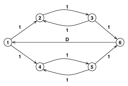
Consider LP (1) with $\alpha=\frac{1}{k}\leq\frac{1}{2}$ for some integer $k\geq 2$. It can be shown that, as a relaxation for the ATSPP problem, this LP has unbounded integrality gap. For example, let $D$ be an arbitrarily large value and consider the shortest path metric obtained from the graph in Figure 1. One can verify that the following assignment of $x$-values to the arcs is feasible for LP (1) with $\alpha=\nicefrac{{1}}{{2}}$. Assign a value of $\nicefrac{{1}}{{2}}$ to arcs $(1,2)$, $(3,2)$, $(3,6)$, $(1,4)$, $(5,4)$, and $(5,6)$ and a value of 1 to arcs $(2,3)$ and $(4,5)$. Every other arc is assigned a value of 0. This assignment is feasible for the linear program and has objective function value 5. On the other hand, any Hamiltonian path from 1 to 6 has cost at least $D$.

Let $L$ be the cost of the optimal solution to LP($\alpha=\frac{1}{k}$). We show how to find $k\cdot\log n$ paths from $s$ to $t$, such that each node of $G$ appears on at least one path, and the total cost of all these paths is at most $k\log n\cdot L$. Let us define a $k$-path-cycle cover to be a set of $k$ disjoint paths from $s$ to $t$ and zero or more cycles, which together cover all nodes. Like a path-cycle cover, the minimum-cost $k$-path-cycle cover can be found by a combinatorial algorithm by creating $k$ copies of both $s$ and $t$ and using the matching algorithm described in [20].

In this section we consider the $k$-person asymmetric traveling salesman path problem. The LP relaxation for this problem is similar to LP (1), but with $x(\delta^{+}(s))=x(\delta^{-}(t))=k$ for constraint (3) and $x(\delta^{-}(S))\geq 1$ for constraint (5). Arguments similar to those in Section 2 show that a $k$-path-cycle cover on any subset $W$ is a lower bound on the value of the LP relaxation for the $k$-person ATSPP. Our algorithm constructs a solution that uses each edge of $O(k\log n)$ $k$-path-cycle covers at most $k$ times, proving a bound of $O(k^{2}\log n)$ on the approximation ratio and the integrality gap.

Our algorithm starts by running lines 1-16 of Algorithm 1, except with $T=(k+1)\log n+1$ iterations of the loop and finding minimum-cost $k$-path-cycle covers instead of the path-cycle covers on line 3. Then it finds $k$ $s$-$t$ paths in the resulting acyclic graph $F$, satisfying conditions of Lemma 5.1 below. The algorithm concludes by incorporating each component of the circulation $H$ into one of the obtained paths, similarly to lines 18-21 of Algorithm 1.

Let $K$ be the comparability graph obtained from $F$. Namely, $K$ has the same set of nodes as $F$, and there is an undirected edge between nodes $u$ and $v$ in $K$ if $F$ contains a directed path either from $u$ to $v$ or from $v$ to $u$. We claim that the nodes of $K$ can be partitioned into at most $k$ cliques. As comparability graphs are perfect graphs [14], the minimum number of cliques that $K$ can be partitioned into is equal to the size of the maximum independent set in $K$. So suppose, for the sake of contradiction, that $K$ contains an independent set $I$ of size $k+1$. Then no nodes in $I$ must share any of the paths in our decomposition of $F$. Since each appears on at least $T-\log n$ paths, there must be at least $(k+1)\cdot(T-\log n)$ paths total in the decomposition. However, this is a contradiction, since $(k+1)\cdot(T-\log n)=(k+1)k\log n+k+1>(k+1)k\log n+k=kT$.

Given the set of $k$ cliques in $K$, we can convert each of them into an $s$-$t$ path in $F$. For each such clique $C$, order the nodes of $C$ in a way consistent with a topological ordering of $F$. Then $F$ contains a path from each node $u$ of $C$ to the next node $v$: the existence of a $uv$ edge in $K$ shows that there is a path between these nodes in $F$, and the topological ordering guarantees that this path goes in the correct direction. There must also be paths from $s$ to the first node of $C$ as well as from the last node of $C$ to $t$, since $s$ is the only source and $t$ is the only sink of $F$. Furthermore, the acyclicity of $F$ shows that each edge of $F$ is used at most once for connecting nodes in $C$. As there are $k$ cliques, each edge is used at most $k$ times in total. If the number of cliques is smaller than $k$, then we can add arbitrary paths from $F$ to our collection to obtain exactly $k$ paths.

To find the required paths algorithmically, we construct the following bipartite graph $B$ from $F$ with bipartitions $X$ and $Y$. For each $v\in F\setminus\{s,t\}$, add nodes $x_{v}$ to $X$ and $y_{v}$ to $Y$ (note that $|X|=|Y|$). Now, for each ordered pair of nodes $(u,v)$ such that there is a directed path from $u$ to $v$ in $F$, add an edge from $x_{u}$ to $y_{v}$. Let $K^{\prime}$ be the directed graph obtained from $K-\{s,t\}$ by orienting each edge $uv$ according to flow $F$. It is easy to see that any collection of $q$ disjoint cliques covering $K-\{s,t\}$ corresponds to a covering of $K^{\prime}$ by $q$ vertex-disjoint paths and vice-versa. We claim that there is a covering of $K^{\prime}$ by $q$ disjoint paths if and only if there is a matching in $B$ that leaves only $q$ nodes in $X$ and $q$ nodes in $Y$ unmatched.

Consider a covering of $K^{\prime}$ by $q$ vertex-disjoint paths $P$. Form a matching $M=\{x_{u}y_{v}:uv\rm{~used~by~}P\}$. Since $P$ is a collection of vertex-disjoint paths, each node has indegree and outdegree at most one in $P$, so $M$ is a valid matching. Furthermore, since $P$ covers the nodes of $K^{\prime}$ with $q$ paths, then exactly $q$ nodes have indegree 0 and exactly $q$ nodes have outdegree 0. Thus, in $M$ exactly $q$ nodes of $X$ and $q$ nodes of $Y$ are unmatched. Conversely, let $M$ be a matching of $B$ that leaves exactly $q$ nodes of $X$ unmatched. For each unmatched node $y_{u}\in Y$, form a directed path in $K^{\prime}$ starting at $u$ by the following process. If $x_{u}$ is matched to, say, $y_{v}$, then add arc $uv$ to the path. Continue this process from $y_{v}$ until the corresponding node in $X$ is not matched. This will form $q$ vertex-disjoint paths in $K^{\prime}$ that cover all nodes.

As noted earlier, we know that $K$ can be covered by at most $k$ disjoint cliques. Therefore, there is a matching in $B$ that leaves at most $k$ nodes in $X$ and $k$ nodes in $Y$ unmatched. Compute such a matching and map it to the corresponding paths in $K^{\prime}$. Finally, extend these at most $k$ paths to $s-t$ paths by adding an arc from $s$ to the start of each path and an arc from the end of each path to $t$. Again, since the only source in $F$ is $s$ and the only sink in $F$ is $t$, these arcs correspond to edges in $K$. $\Box$

We introduce LP relaxation (8) for the directed latency problem. The use of $x_{uw}$ and $f^{v}_{uw}$ variables in an integer programming formulation for directed latency was proposed by Mendez-Diaz et al. [22], who do a computational evaluation of the strength of its LP relaxation. However, our LP formulation uses a different set of constraints than the one in [22].

In LP (8), a variable $x_{uw}$ indicates that node $u$ appears before node $w$ on the path. Similarly, $x_{uvw}$ for three distinct nodes $u$, $v$, $w$ indicates that they appear in this order on the path. For every node $v\neq s$, we send one unit of flow from $s$ to $v$, and we call it the $v$-flow. Then $f^{v}_{uw}$ is the amount of $v$-flow going through edge $(u,w)$, and $\ell(v)$ is the latency of node $v$. To show that this LP is a relaxation of the directed latency problem, given a solution path $P$, we can set $f^{v}_{uw}=1$ whenever the edge $(u,w)$ is in $P$ and $v$ occurs later than $u$ in $P$, and $f^{v}_{uw}=0$ otherwise. So $f^{v}$ is one unit of flow from $s$ to $v$ along the path $P$. Also setting the ordering variables $x_{uw}$ and $x_{uvw}$ to 0 or 1 appropriately and setting $\ell(v)$ to the latency of $v$ in $P$, we get a feasible solution to LP (8) of the same cost as the total latency of $P$.

Constraints (12) are the flow conservation constraints for $v$-flow at node $u$. Constraints (13) ensure that no $v$-flow enters $s$ or leaves $v$. Constraints (14) say that $v$-flow passes through $u$ if and only if $u$ occurs before $v$. Since the $t$-flow goes through every vertex, when all the variables are in $\{0,1\}$, it defines an $s$-$t$ path. We can think of the $t$-flow as the universal flow and Constraints (15) ensure that every $v$-flow follows an edge which has a universal flow on it. Constraints (16), in an integer solution, ensure that if a set $S$ contains some node $y$ that comes before $v$ (i.e. $x_{yv}=1$), then at least one unit of $v$-flow enters $S$.

We note that a min-cut subroutine can be used to detect violated constraints of type (16), allowing us to solve LP (8) using the ellipsoid method. Our analysis does not actually use Constraints (15), so we can drop them from the LP. Although without these constraints the corresponding integer program may not be an exact formulation for the directed latency problem, we can still find a solution whose cost is within factor $O(\log n)$ of this relaxed LP.

Using Lemma 6.1 and scaling the edge lengths (if needed), we can assume that we have a solution $({x},{\ell},{f})$ satisfying the following:

The idea of our algorithm is to construct $s$-$v$ paths for several nodes $v$, such that together they cover all vertices of $V$, and then to “stitch” these paths together to obtain one Hamiltonian path. We use our results for ATSPP to construct these paths. For this, we observe that parts of a solution to the latency LP (8) can be transformed to obtain feasible solutions to different instances of LP($\alpha$). For example, we can construct a Hamiltonian $s$-$t$ path of total length $O(\log n)\cdot\ell(t)$ as follows. From a solution to LP (8), take the $t$-flow defined by the variables $f^{t}_{uw}$, and notice that it constitutes a feasible solution to LP($\alpha=1$). In particular, since $x_{yt}=1$ for all $y$, constraints (16) of LP (8) for $v=t$ imply that the set constraints (5) of LP (1) are satisfied. The objective function value for LP (1) of this solution is at most $\ell(t)$. Thus, by Theorem 1.1, we can find the desired path. Of course, this path is not yet a good solution for the latency problem, as even nodes $v$ with $\ell(v)\ll\ell(t)$ can have latency in this path close to $O(\log n)\cdot\ell(t)$. Our algorithm constructs several paths of different lengths, incorporating most nodes $v$ into paths of length $O(\log n)\cdot\ell(v)$, and then combines these paths to obtain the final solution.

References

- [1] F. N. Afrati, S. S. Cosmadakis, C. H. Papadimitriou, G. Papageorgiou, and N. Papakostantinou. The complexity of the travelling repairman problem. Informatique Theorique et Applications, 20(1):79–87, 1986.
- [2] A. Archer, A. Levin, and D. P. Williamson. A faster, better approximation algorithm for the minimum latency problem. SIAM J. Comput., 37(5):1472–1498, 2008.
- [3] A. Asadpour, M. X. Goemans, A. Madry, S. Oveis Gharan, and A. Saberi. An -approximation algorithm for the asymmetric traveling salesman problem. In Proc. 21st ACM Symp. on Discrete Algorithms, 2010.
- [4] A. Blum, P. Chalasani, D. Coppersmith, B. Pulleyblank, P. Raghavan, and M. Sudan. The minimum latency problem. In Proc. 26th ACM Symp. on Theory of Computing, 1994.
- [5] M. Charikar, M. X. Goemans, and H. Karloff. On the integrality ratio for asymmetric TSP. In Proc. 45th IEEE Symp. on Foundations of Computer Science, 2004.
- [6] K. Chaudhuri, B. Godfrey, S. Rao, and K. Talwar. Paths, trees, and minimum latency tours. In Proc. 44th IEEE Symp. on Foundations of Computer Science, 2003.
- [7] C. Chekuri and M. Pal. An approximation ratio for the asymmetric traveling salesman path problem. Theory of Computing, 3(1):197–209, 2007.
- [8] N. Christofides. Worst-case analysis of a new heuristic for the traveling salesman problem. Technical report, Graduate School of Industrial Administration, Carnegie-Mellon University, Pittsburgh, PA, 1976.
- [9] U. Feige and M. Singh. Improved approximation ratios for traveling salesperson tours and paths in directed graphs. In Proc. 10th APPROX, 2007.
- [10] A. Frank. On connectivity properties of Eulerian digraphs. Ann. Discrete Math., 41:179–194, 1989.
- [11] A. Frieze, G. Galbiati, and F. Maffioli. On the worst-case performance of some algorithms for the asymmetric traveling salesman problem. Networks, 12:23–39, 1982.
- [12] A. M. Frieze. An extension of Christofides heuristic to the k-person travelling salesman problem. Discrete Applied Mathematics, 6(1):79–83, 1983.
- [13] M. Goemans and J. Kleinberg. An improved approximation ratio for the minimum latency problem. Math. Program., 82:111–124, 1998.
- [14] M. C. Golumbic. Algorithmic Graph Theory and Perfect Graphs (Annals of Discrete Mathematics, Vol 57). North-Holland Publishing Co., Amsterdam, The Netherlands, second edition, 2004.
- [15] G. Gutin and A. P. Punnen, editors. Traveling Salesman Problem and Its Variations. Springer, Berlin, 2002.
- [16] J. A. Hoogeveen. Some paths are more difficult than cycles. Oper. Res. Lett., 10:291–295, 1991.
- [17] B. Jackson. Some remarks on arc-connectivity, vertex splitting, and orientation in digraphs. Journal of Graph Theory, 12(3):429–436, 1988.
- [18] H. Kaplan, M. Lewenstein, N. Shafrir, and M. Sviridenko. Approximation algorithms for asymmetric TSP by decomposing directed regular multigraphs. J. ACM, 52(4):602–626, 2005.
- [19] J. Kleinberg and D. P. Williamson. Unpublished note, 1998.
- [20] F. Lam and A. Newman. Traveling salesman path problems. Math. Program., 113(1):39–59, 2008.
- [21] E. Lawler, J. K. Lenstra, A. H. G. Rinnooy Kan, and D. Shmoys, editors. The Traveling Salesman Problem: A guided tour of combinatorial optimization. John Wiley & Sons Ltd., 1985.
- [22] I. Mendez-Diaz, P. Zabala, and A. Lucena. A new formulation for the traveling deliveryman problem. Discrete Applied Mathematics, 156(17):3223–3237, 2008.
- [23] E. Minieka. The deliveryman problem on a tree network. Ann. Oper. Res., 18:261–266, 1989.
- [24] V. Nagarajan and R. Ravi. Poly-logarithmic approximation algorithms for directed vehicle routing problems. In Proc. 10th APPROX, pages 257–270, 2007.
- [25] V. Nagarajan and R. Ravi. The directed minimum latency problem. In Proc. 11th APPROX, pages 193–206, 2008.
- [26] C. H. Papadimitriou and S. Vempala. On the approximability of the traveling salesman problem. Combinatorica, 26(1):101–120, 2006.
- [27] D. Shmoys and D. P. Williamson. Analyzing the Held-Karp TSP bound: a monotonicity property with application. Inf. Process. Lett., 35(6):281–285, 1990.
- [28] D. P. Williamson. Analysis of the Held-Karp heuristic for the traveling salesman problem. M.S. Thesis, MIT, 1990.
- [29] L. A. Wolsey. Heuristic analysis, linear programming and branch and bound. Mathematical Programming Study, 13:121–134, 1980.