Asymptotic analysis of a family of polynomials associated with the inverse error function

The error function $\operatorname{erf}(x)$ is defined by [1]

$$\operatorname{erf}(x)=\frac{2}{\sqrt{\pi}}\int\limits_{0}^{x}\exp\left(-t^{2}\right)dt$$

(1)

and its inverse $\operatorname*{inverf}\left(x\right)$, which we will denote by $\mathfrak{I}(x),$ satisfies $\mathfrak{I}\left[\operatorname{erf}(x)\right]=\operatorname{erf}\left[\mathfrak{I}(x)\right]=x.$ The function $\mathfrak{I}(x)$ appears in several problems of heat conduction [12]. In [10] we considered the function

$$N(x)=\frac{1}{\sqrt{2\pi}}\int_{-\infty}^{x}e^{-t^{2}/2}dt$$

(2)

and its inverse $S(x),$ satisfying

$$S\left[N(x)\right]=N\left[S(x)\right]=x.$$

It is clear from (1) and (2) that

$$N(x)=\frac{1}{2}\left[\operatorname{erf}\left(\frac{x}{\sqrt{2}}\right)+1\right]$$

and therefore

$$S(x)=\sqrt{2}\mathfrak{I}\left(2x-1\right).$$

(3)

In [10] we showed that

$$S^{\prime}(x)=\sqrt{2\pi}\exp\left[\frac{1}{2}S^{2}(x)\right]$$

(4)

and

$$S^{(n)}=P_{n-1}(S)(S^{\prime})^{n}\quad n\geq 1,$$

(5)

where $P_{n}(x)$ is a polynomial of degree $n$ satisfying the recurrence

$$P_{0}(x)=1,\quad P_{n+1}(x)=P_{n}^{\prime}(x)+x(n+1)P_{n}(x),\quad n\geq 1.$$

(6)

The same approach was employed by Carlitz in [2]. From (6), it follows easily that for a fixed value of $n$

$$P_{n}(x)\sim n!\,x^{n},\quad x\rightarrow\infty.$$

(7)

From (3) and (5), we conclude that

$$\mathfrak{I}^{(n)}=2^{\frac{n-1}{2}}P_{n-1}\left(\sqrt{2}\mathfrak{I}\right)\left(\mathfrak{I}^{\prime}\right)^{n}\quad n\geq 1.$$

Since

$$\mathfrak{I}(0)=0,\quad\mathfrak{I}^{\prime}(0)=\frac{\sqrt{\pi}}{2},$$

we have

$$\mathfrak{I}^{(n)}(0)=\frac{1}{\sqrt{2}}\left(\frac{\pi}{2}\right)^{\frac{n}{2}}P_{n-1}(0).$$

(8)

It follows from (8) that estimating $\mathfrak{I}^{(n)}(0)$ for large values of $n$ is equivalent to finding an asymptotic approximation of the polynomials $P_{n}(x)$ when $x=0$.

The objective of this work is to study $P_{n}(x)$ asymptotically as $n\rightarrow\infty$ for various ranges of $x.$ We shall obtain different asymptotic expansions for $n\rightarrow\infty$ and (i) $0<x<\infty,$ (ii) $x=O\left(n^{-1}\right)$ and (iii) $x=O\left(\sqrt{\ln(n)}\right).$ The paper is organized as follows: in Section 2 we approach the problem using a singularity analysis of the generating function [14] of the polynomials $P_{n}(x).$ In Section 3 we apply the WKB method to the differential-difference equation (6). In [15], we used this approach in the asymptotic analysis of computer science problems and in [6] to study the Krawtchouk polynomials. Finally, in Section 4 we analyze (6) again using the ray method [13] and obtain an asymptotic approximation valid in various regions of the $(x,n)$ domain. In [4], [5], [7], we employed the same technique to analyze asymptotically other families of polynomials and in [8], [9] to study some queueing problems.

In [10] we obtained the exponential generating function

$$\sum_{n=0}^{\infty}P_{n}(x)\frac{z^{n}}{n!}=\exp\left\{\frac{1}{2}S^{2}[N(x)+zN^{\prime}(x)]-\frac{x^{2}}{2}\right\},$$

which implies that

$$P_{n}(x)=e^{-x^{2}/2}\frac{n!}{2\pi\mathrm{i}}\oint\limits_{\left|z\right|<r}\exp\left\{\frac{1}{2}S^{2}[N(x)+zN^{\prime}(x)]\right\}\frac{dz}{z^{n+1}},$$

where the integration contour is a small loop around the origin in the complex plane. Using (4), we have

	$\displaystyle P_{n}(x)$	$\displaystyle=e^{-x^{2}/2}\frac{n!}{2\pi\mathrm{i}}\oint\limits_{\left|z\right|<r}\frac{1}{\sqrt{2\pi}}S^{\prime}[N(x)+zN^{\prime}(x)]\frac{dz}{z^{n+1}}$
		$\displaystyle=e^{-x^{2}/2}\frac{1}{\sqrt{2\pi}N^{\prime}(x)}\frac{n!}{2\pi\mathrm{i}}\oint\limits_{\left|z\right|<r}\frac{1}{z^{n+1}}dS[N(x)+zN^{\prime}(x)]$
		$\displaystyle=\frac{n!}{2\pi\mathrm{i}}\oint\limits_{\left|z\right|<r}\frac{n+1}{z^{n+2}}S[N(x)+zN^{\prime}(x)]dz$

and therefore

$$P_{n}(x)=\frac{\left(n+1\right)!}{2\pi\mathrm{i}}\oint\limits_{\left|z\right|<r}S[N(x)+zN^{\prime}(x)]\frac{dz}{z^{n+2}}.$$

(9)

Since $S(x)$ has singularities at $x=0$ and $x=1,$ we consider the functions

$$Z_{1}(x)=\frac{1-N(x)}{N^{\prime}(x)},\quad Z_{0}(x)=-\frac{N(x)}{N^{\prime}(x)}.$$

We have

$$Z_{1}(-x)=-\sqrt{2\pi}\exp\left(\frac{x^{2}}{2}\right)-Z_{1}(x)$$

(10)

and

	$\displaystyle Z_{1}(x)$	$\displaystyle=x^{-1}+O\left(x^{-3}\right),\quad x\rightarrow\infty,$
	$\displaystyle\quad Z_{0}(x)$	$\displaystyle=-\sqrt{2\pi}\exp\left(\frac{x^{2}}{2}\right)+x^{-1}+O\left(x^{-3}\right),\quad x\rightarrow\infty.$

Changing variables to

$$w=\left[z-Z_{1}(x)\right]N^{\prime}(x)$$

in (9), we obtain

$$P_{n}(x)=\frac{1}{N^{\prime}(x)}\frac{\left(n+1\right)!}{2\pi\mathrm{i}}\oint\limits_{C}S\left(w+1\right)\left[\frac{w}{N^{\prime}(x)}+Z_{1}(x)\right]^{-(n+2)}dw,$$

or,

$$P_{n}(x)=\sqrt{\pi}e^{x^{2}/2}\frac{\left(n+1\right)!}{2\pi\mathrm{i}}\oint\limits_{C}\frac{\mathcal{J}\left(w+1\right)}{\left[\sqrt{\frac{\pi}{2}}e^{x^{2}/2}w+Z_{1}(x)\right]^{n+2}}dw,$$

(11)

where $C$ is a small loop about $w=w^{\ast}(x)$ in the complex plane, with

$$w^{\ast}(x)=-\sqrt{\frac{2}{\pi}}e^{-x^{2}/2}Z_{1}(x).$$

To expand (11) for $n\rightarrow\infty$ with a fixed $x\in\left(0,\infty\right),$ we employ singularity analysis. The function $\mathcal{J(}w)$ has singularities at $w=\pm 1.$ By (1), we have

$$w=\frac{2}{\sqrt{\pi}}\int\limits_{0}^{\mathcal{J}}e^{-t^{2}}dt=1-e^{-\mathcal{J}^{2}}\left[\frac{1}{\sqrt{\pi}\mathcal{J}}+O\left(\mathcal{J}^{-3}\right)\right],\quad\mathcal{J}\rightarrow\infty,$$

so that

$$\mathcal{J(}w)\sim\sqrt{-\ln(1-w)},\quad w\rightarrow 1^{-}$$

and by symmetry we have

$$\mathcal{J(}w)\sim-\sqrt{-\ln(1+w)},\quad w\rightarrow-1^{+}.$$

The integrand in (11) thus has singularities at $w=0$ and $w=-2,$ but for $x>0,$ the former is closer to $w^{\ast}(x).$ We expand (11) around $w=0$ by setting $w=\delta/n$ and using

$$\left[Z_{1}(x)+\sqrt{\frac{\pi}{2}}e^{x^{2}/2}\frac{\delta}{n}\right]^{-(n+2)}\sim\left[Z_{1}(x)\right]^{-(n+2)}\exp\left[-\sqrt{\frac{\pi}{2}}e^{x^{2}/2}\frac{\delta}{Z_{1}(x)}\right].$$

(12)

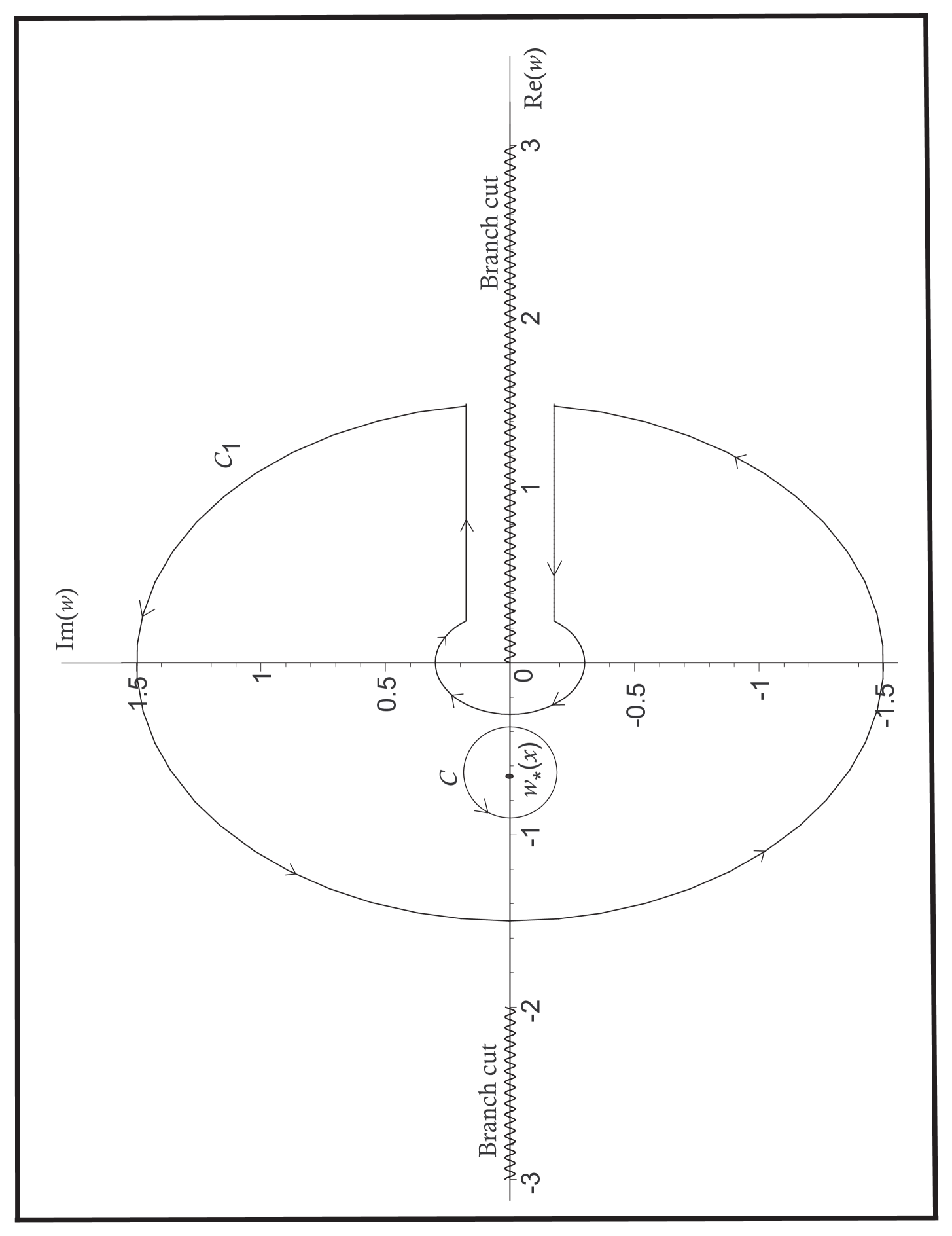
Then, we deform the contour $C$ in (11) to a new contour $C_{1}$ that encircles the branch point at $w=0$ (see Figure 1). This leads to

	$\displaystyle P_{n}(x)$	$\displaystyle\sim\left(n+1\right)!\sqrt{\pi}e^{x^{2}/2}\left[Z_{1}(x)\right]^{-(n+2)}\frac{1}{n}$		(13)
		$\displaystyle\times\frac{1}{2\pi\mathrm{i}}\int\limits_{0}^{\infty}\left(\Upsilon^{+}-\Upsilon^{-}\right)\exp\left[-\sqrt{\frac{\pi}{2}}\frac{e^{x^{2}/2}}{Z_{1}(x)}\delta\right]d\delta,$

where

$$\Upsilon^{\pm}(\delta,n)=\sqrt{\pm\mathrm{i}\pi-\ln\left(\delta\right)+\ln\left(n\right)}.$$

Here $\Upsilon^{\pm}(\delta,n)$ corresponds to the approximation of $\mathcal{J(}w+1)$ for $w\rightarrow 0,$ above or below the right branch cut in Figure 1.

For $n$ large we have

$$\Upsilon^{+}(\delta,n)-\Upsilon^{-}(\delta,n)\sim\frac{\pi\mathrm{i}}{\sqrt{\ln\left(n\right)}}$$

and then evaluating the elementary integral in (13) leads to $P_{n}(x)\sim\Psi_{1}(x,n)$ as $n\rightarrow\infty$ with

$$\Psi_{1}(x,n)=\frac{n!}{\sqrt{2\ln\left(n\right)}}\left[Z_{1}(x)\right]^{-\left(n+1\right)}=\frac{n!}{\sqrt{2\ln\left(n\right)}}\left[\frac{e^{-x^{2}/2}}{\zeta\left(x\right)}\right]^{n+1}$$

(14)

and

$$\zeta\left(x\right)=\sqrt{\frac{\pi}{2}}\left[1-\operatorname*{erf}\left(\frac{x}{\sqrt{2}}\right)\right]\sim\exp\left(-\frac{x^{2}}{2}\right)\left[x^{-1}+O\left(x^{-3}\right)\right],\quad x\rightarrow\infty.$$

(15)

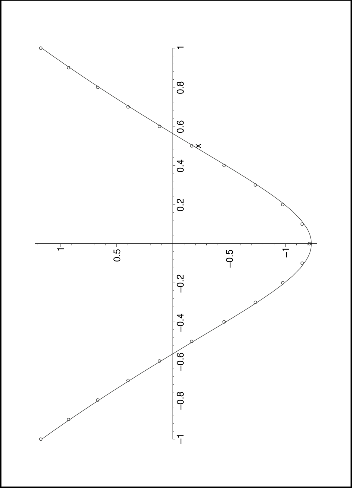
In Figure 2 we plot $\ln\left[P_{40}(x)/40!\right]$ and $\ln\left[\Psi_{1}(x,40)/40!\right]$. We see that the approximation is very good for $x=O(1)$ but it becomes less precise as $x\rightarrow\infty.$ This is because our previous analysis assumes that $n\rightarrow\infty$ with $0<x<\infty.$ If either $x\rightarrow 0$ or $x\rightarrow\infty,$ we must modify it, which we will do next.

When $x\rightarrow 0,$ or more generally when $x=O\left(n^{-1}\right),$ the singularities at $w=0$ and $w=-2$ are nearly equidistant from $w^{\ast}(x).$ On the scale $x=y/n,$ $y=O\left(1\right),$ we have

$$Z_{1}(x)=Z_{1}\left(\frac{y}{n}\right)=\sqrt{\frac{\pi}{2}}-\frac{y}{n}+O\left(n^{-2}\right),\quad n\rightarrow\infty$$

(16)

and (14) simplifies to

$$P_{n}(x)\sim\frac{n!}{\sqrt{2\ln\left(n\right)}}\left(\sqrt{\frac{2}{\pi}}\right)^{n+1}\exp\left(y\sqrt{\frac{2}{\pi}}\right).$$

(17)

But, to this we must add the contribution from $w=-2,$ which corresponds to replacing $y$ by $-y$ and multiplying by $\left(-1\right)^{n}$ the right hand side of (17).

We note from (10) that

$$\sqrt{\frac{\pi}{2}}e^{x^{2}/2}w+Z_{1}(-x)=\sqrt{\frac{\pi}{2}}e^{x^{2}/2}\left(w+2\right)-Z_{1}(x),$$

so that the integrand in (11) is antisymmetric with respect to the map $\left(x,w\right)\rightarrow\left(-x,-2-w\right).$ Thus, for $n\rightarrow\infty$ and $x=O\left(n^{-1}\right)$ we get $P_{n}(x)\sim\Psi_{2}(x,n)$ with

$$\Psi_{2}(y,n)=\frac{n!}{\sqrt{2\ln\left(n\right)}}\left(\sqrt{\frac{2}{\pi}}\right)^{n+1}\left[\exp\left(y\sqrt{\frac{2}{\pi}}\right)+\left(-1\right)^{n}\exp\left(-y\sqrt{\frac{2}{\pi}}\right)\right].$$

(18)

As $y\rightarrow\infty,$ the alternating term becomes negligible and (18) matches to (14), as $x\rightarrow 0.$ In Figure 3 we plot the ratio $\ln\left[P_{40}\left(\frac{y}{40}\right)/40!\right]/\ln\left[\Psi_{2}(y,40)/40!\right]$ and verify the accuracy of (18).

Letting $x\rightarrow\infty$ in (13) using (14) yields

$$P_{n}(x)\sim\frac{n!\,x^{n+1}}{\sqrt{2\ln(n)}},$$

which differs from (7). This suggests that another scale must be analyzed, where $x$ and $n$ are both large. Thus, we consider the case of $x\rightarrow\infty$, with $x=O\left(\sqrt{\ln n}\right).$ Now the singularity at $w=0$ in (11) becomes close to $w^{\ast}(x),$ since

$$w^{\ast}(x)\sim-\frac{\sqrt{2}}{x\sqrt{\pi}},\quad x\rightarrow\infty.$$

we use the form (9) and expand $S[N(x)+zN^{\prime}(x)]$ for $z\rightarrow 0$ and $x\rightarrow\infty.$ Setting $z=\xi/x$ with $\xi=O(1),$ we obtain

	$$\displaystyle S[N(x)+zN^{\prime}(x)]=\sqrt{2}\mathcal{J}\left\{1+\sqrt{\frac{2}{\pi}}\left[ze^{-x^{2}/2}-\zeta\left(x\right)\right]\right\}$$
	$$\displaystyle=\sqrt{2}\mathcal{J}\left[1+\sqrt{\frac{2}{\pi}}e^{-x^{2}/2}\left(z-\frac{1}{x}+O\left(x^{-3}\right)\right)\right]$$
	$$\displaystyle\sim\sqrt{2}\sqrt{-\ln\left[\sqrt{\frac{2}{\pi}}e^{-x^{2}/2}\left(\frac{1}{x}-z\right)\right]}$$
	$$\displaystyle\sim\sqrt{2}\sqrt{\frac{x^{2}}{2}+\ln(x)-\frac{1}{2}\ln\left(\frac{2}{\pi}\right)-\ln\left(1-\xi\right)}.$$

Thus, we have

$$P_{n}(x)\sim\frac{\sqrt{2}\left(n+1\right)!x^{n+1}}{2\pi\mathrm{i}}\oint\limits_{C_{1}}\sqrt{\frac{x^{2}}{2}+\ln\left(\frac{x}{1-\xi}\right)-\frac{1}{2}\ln\left(\frac{2}{\pi}\right)}\frac{d\xi}{\xi^{n+2}}.$$

(19)

Here the contour $C_{1}$ is a small loop about $\xi=0.$ Now we again employ singularity analysis, with the branch point at $\xi=1$ determining the asymptotic behavior for $n\rightarrow\infty.$ A deformation similar to that in Figure 1 leads to

$$P_{n}(x)\sim\frac{n!x^{n+1}}{\sqrt{2}}\frac{1}{\sqrt{\frac{x^{2}}{2}+\ln(nx)-\frac{1}{2}\ln\left(\frac{2}{\pi}\right)}}.$$

(20)

For $x>>\sqrt{\ln(n)}$ this collapses to (7).

By examining (14) and (20), we can obtain the following approximation

$$P_{n}(x)\sim\Psi_{3}(x,n)=\frac{n!}{\sqrt{x^{2}+2\ln(nx)-\ln\left(\frac{2}{\pi}\right)}}\left[\frac{e^{-x^{2}/2}}{\zeta\left(x\right)}\right]^{n+1},$$

(21)

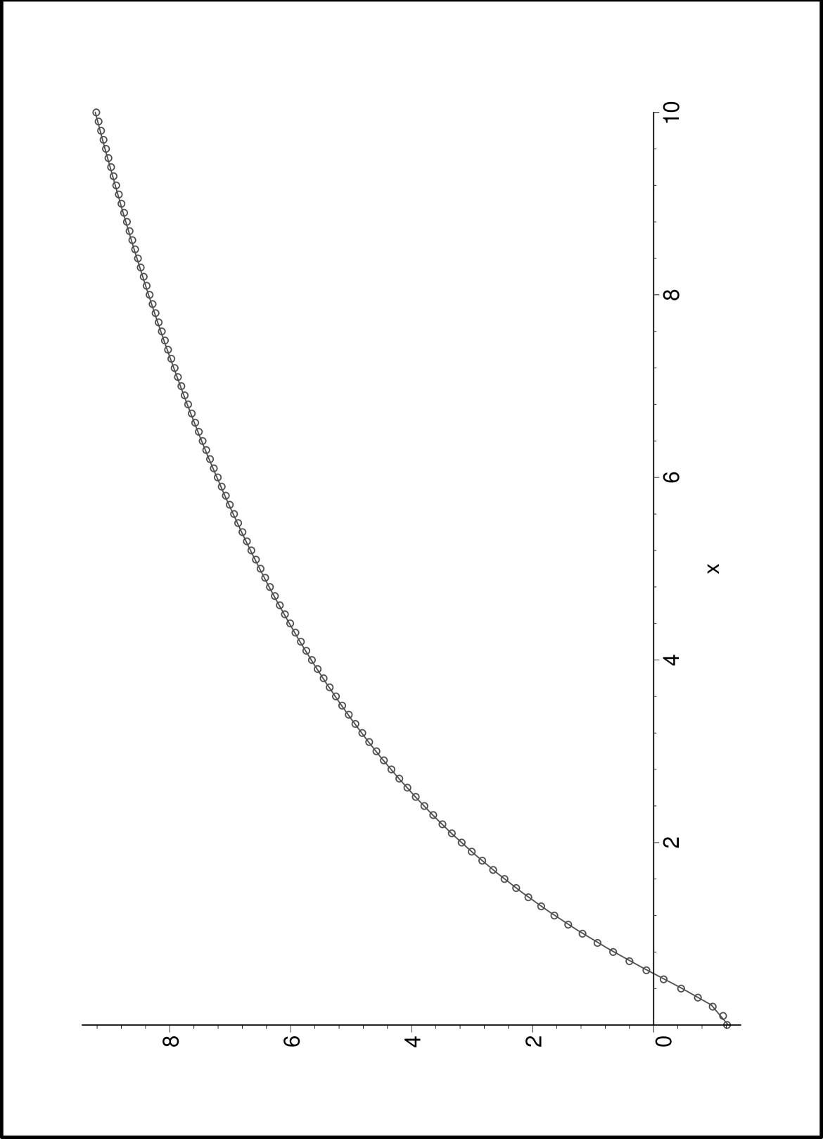
which is more uniform in $x$, since it holds both for $x=O(1)$ and $x=O\left(\sqrt{\ln n}\right)$ for $n$ large and for $x\rightarrow\infty$ with $n$ fixed. However, we must still use (18) if $n$ is large and $x$ is small. In Figure 4 we plot $\ln\left[P_{40}(x)/40!\right]$ and $\ln\left[\Psi_{3}(x,40)/40!\right]$ and confirm that (21) is a better approximation than (14) for large values of $x.$

We shall now rederive the results in the previous section by using only the recurrence (6) and (7). We apply the WKB method to (6), seeking solutions of the form $P_{n}(x)=n!\overline{P}_{n}(x),$ with

$$\overline{P}_{n}(x)\sim\exp\left[\left(n+1\right)A(x)\right]B(x,n),\quad n\rightarrow\infty.$$

(22)

Thus, we are assuming an exponential dependence on $n$ and an additional weaker (e.g., algebraic) dependence that arises from the function $B(x,n).$ Using (22) in (6) leads to

	$\displaystyle e^{A(x)}\left[B(x,n)+\frac{\partial}{\partial n}B(x,n)\right]+O\left(\frac{\partial^{2}B}{\partial n^{2}}\right)$
	$\displaystyle=\left[x+A^{\prime}(x)\right]B(x,n)+\frac{1}{n+1}\frac{\partial}{\partial x}B(x,n).$

Expecting that $\frac{\partial B}{\partial n}=o\left(B\right)$ and $\frac{\partial^{2}B}{\partial n^{2}}=o\left(\frac{\partial B}{\partial n}\right),$ we set

$$e^{A(x)}=x+A^{\prime}(x)$$

(23)

and

$$e^{A(x)}\frac{\partial}{\partial n}B(x,n)=\frac{1}{n+1}\frac{\partial}{\partial x}B(x,n)\sim\frac{1}{n}\frac{\partial}{\partial x}B(x,n).$$

(24)

To solve (23) we let

$$A(x)=-\frac{x^{2}}{2}+a(x)$$

to find that

$$a^{\prime}(x)=e^{-x^{2}/2}e^{a(x)}.$$

Solving this separable ODE leads to

$$A(x)=-\frac{x^{2}}{2}-\ln\left[\zeta\left(x\right)+k\right],$$

(25)

where $k$ is a constant of integration. To fix $k,$ we assume that expansion (22), as $x\rightarrow\infty,$ will asymptotically match to (7), when this is expanded for $n\rightarrow\infty.$ In view of (22) this implies that

$$\overline{P}_{n}(x)\sim x^{n}=\exp\left[n\ln(x)\right],\quad x\rightarrow\infty,$$

so that

$$A(x)\sim\ln(x),\quad x\rightarrow\infty.$$

In view of (25) this is possible only if $k=0$ and then from (15) we have

$$A(x)=-\ln\left[e^{x^{2}/2}\zeta\left(x\right)\right]\sim\ln(x),\quad x\rightarrow\infty.$$

(26)

We next analyze (24). Using (26) to compute $e^{A(x)},$ we obtain

$$\frac{e^{-x^{2}/2}}{\zeta\left(x\right)}\frac{\partial}{\partial n}B(x,n)=\frac{1}{n}\frac{\partial}{\partial x}B(x,n).$$

Solving this first order PDE by the method of characteristics, we obtain

$$B(x,n)=b\left[\frac{n}{\zeta\left(x\right)}\right],$$

where $b\left(\cdot\right)$ is at this point an arbitrary function. However, since $n$ is large and $x=O(1),$ we need only the behavior of $b\left(\cdot\right)$ for large values of its argument. We again argue that by matching to (7) we have

$$\exp\left[\left(n+1\right)A(x)\right]B(x,n)\sim x^{n},\quad x\rightarrow\infty,$$

and using (26) we get

$$B(x,n)\sim e^{-A(x)}\sim\frac{1}{x},\quad x\rightarrow\infty$$

and thus

$$b\left(nxe^{x^{2}/2}\right)\sim\frac{1}{x},\quad x\rightarrow\infty$$

so that

$$b(z)\sim\frac{1}{\sqrt{2\ln(z)}},\quad z\rightarrow\infty.$$

Combining our results, we have found that

$$P_{n}(x)\sim\frac{n!}{\sqrt{2}\sqrt{\ln(n)-\ln\left[\zeta\left(x\right)\right]}}\left[\frac{e^{-x^{2}/2}}{\zeta\left(x\right)}\right]^{n+1},\quad n\rightarrow\infty.$$

(27)

This applies for $x=O(1)$ and $n\rightarrow\infty,$ where we can regain the results of the singularity analysis (14) by simply using

$$\sqrt{\ln(n)-\ln\left[\zeta\left(x\right)\right]}\sim\sqrt{\ln(n)},\quad n\rightarrow\infty.$$

Formula (27) is also valid for $n=O(1)$ and $x\rightarrow\infty,$ where it reduces to (7). However, (22) breaks down for $x\rightarrow 0.$

We thus consider the scale $x=y/n,$ $y=O\left(1\right)$ and set

$$P_{n}(x)=n!\widetilde{P}_{n}(nx)=n!\widetilde{P}_{n}(y),$$

(28)

with which (6) becomes

$$\widetilde{P}_{n+1}\left(y+\frac{y}{n}\right)=\frac{n}{n+1}\widetilde{P}_{n}^{\prime}(y)+\frac{y}{n}\widetilde{P}_{n}(y).$$

(29)

For fixed $y,$ we seek an asymptotic solution of (29) in the form

$$\widetilde{P}_{n}(y)\sim e^{\alpha n}q\left(y,n\right),\quad n\rightarrow\infty,$$

(30)

where $q\left(y,n\right)$ will have a weaker (e.g., algebraic or logarithmic) dependence on $n.$ From (29) we obtain, using (30),

	$\displaystyle e^{\alpha}\left[q(y,n)+\frac{\partial}{\partial n}q(y,n)+\frac{y}{n}\frac{\partial}{\partial y}q(y,n)+O\left(n^{-2}\right)\right]$		(31)
	$\displaystyle=\left[1-\frac{1}{n}+O\left(n^{-2}\right)\right]\frac{\partial}{\partial y}q(y,n)+\frac{y}{n}q(y,n).$

If $q\left(y,n\right)$ has an algebraic dependence on $n$, then $\frac{\partial}{\partial n}q(y,n)$ should be roughly $O\left(n^{-1}\right)$ relative to $q\left(y,n\right),$ $\frac{\partial^{2}}{\partial n^{2}}q(y,n)$ roughly $O\left(n^{-2}\right)$ and so on. Thus, we expand $q\left(y,n\right)$ as

$$q\left(y,n\right)=q_{0}(y,n)+\frac{1}{n}q_{1}(y,n)+O\left(n^{-2}\right),$$

(32)

where $q_{0}(y,n),q_{1}(y,n)$ have a very weak (e.g., logarithmic) dependence on $n$ and balance terms in (31) of order $O(1)$ and $O\left(n^{-1}\right)$ to obtain

$$e^{\alpha}q_{0}(y,n)=\frac{\partial}{\partial y}q_{0}(y,n)$$

(33)

and

	$\displaystyle e^{\alpha}\left[q_{1}(y,n)+\frac{\partial}{\partial n}q_{1}(y,n)+y\frac{\partial}{\partial y}q_{0}(y,n)\right]$		(34)
	$\displaystyle=\frac{\partial}{\partial y}q_{1}(y,n)-\frac{\partial}{\partial y}q_{0}(y,n)-yq_{0}(y,n).$

Solving (33) yields

$$q_{0}(y,n)=\exp\left(e^{\alpha}y\right)\mathfrak{q}(n),$$

(35)

where $\mathfrak{q}(n)$ must be determined.  We could solve (34), using (35), but its solution would involve another arbitrary function of $n$. Thus, considering higher order terms will not help in determining $\mathfrak{q}(n).$ Instead, we employ asymptotic matching to (27). Expanding (27) for $x\rightarrow 0$ and comparing the result to (28) as $y\rightarrow\infty,$ with (30), (32) and (35), we conclude that

$$\alpha=\frac{1}{2}\ln\left(\frac{2}{\pi}\right),\quad\mathfrak{q}(n)=\frac{1}{\sqrt{\pi\ln(n)}}.$$

(36)

But then our approximation for $y=O(1)$ is not consistent with $P_{n}(0)=0=\widetilde{P}_{n}(0)$ for odd $n.$ We return to (29) and observe that the equation also admits an asymptotic solution of the form

$$\widetilde{P}_{n}(y)\sim\left(-1\right)^{n}e^{\beta n}\overline{q}\left(y,n\right),\quad n\rightarrow\infty$$

where, analogously to (33), we find that

$$-e^{\beta}\overline{q}_{0}(y,n)=\frac{\partial}{\partial y}\overline{q}_{0}(y,n),$$

so that another asymptotic solution to (29) is

$$\widetilde{P}_{n}(y)\sim\left(-1\right)^{n}e^{\beta n}\exp\left(e^{\beta}y\right)\overline{\mathfrak{q}}(n).$$

(37)

We argue that any linear combination of (30) and (37) is also a solution and that the combination which vanishes at $y=0$ for odd $n$ has $\beta=\alpha$ and $\overline{\mathfrak{q}}(n)=\mathfrak{q}(n),$ as in (36). We have thus obtained, for $y=O(1),$

$$P_{n}(x)\sim\frac{n!}{\sqrt{\pi\ln(n)}}\left(\frac{2}{\pi}\right)^{\frac{n}{2}}\left[\exp\left(y\sqrt{\frac{2}{\pi}}\right)+\left(-1\right)^{n}\exp\left(-y\sqrt{\frac{2}{\pi}}\right)\right],\quad n\rightarrow\infty.$$

This agrees with (18), obtained by singularity analysis in section 2.

To summarize, we have shown how to infer the asymptotics of $P_{n}(x)$ using only the recursion (6) and the large $x$ behavior (7). Our analysis does need to make some assumptions about the forms of various expansions and the asymptotic matching between different scales.

We shall now find a uniform asymptotic approximation for $P_{n}(x)$ using a discrete form of the ray method [11]. This approximation will apply for $x$ and/or $n$ large. We seek an approximate solution for (6) of the form

$$P_{n}(x)=\exp\left[f(x,n)+g(x,n)\right],$$

(38)

where $g=o(f)$ as $n\rightarrow\infty.$ Since $P_{n}(x)=x^{n},$ $n=0,1$ we see that we must have

$$f(x,n)\sim n\ln(x)\text{ \ \ and \ \ }g(x,n)\rightarrow 0$$

(39)

as $n\rightarrow 0.$ Using (38) in (6), we have

$$\exp\left(\frac{\partial f}{\partial n}+\frac{1}{2}\frac{\partial^{2}f}{\partial n^{2}}+\frac{\partial g}{\partial n}\right)\sim\left(\frac{\partial f}{\partial x}+\frac{\partial g}{\partial x}\right)+\left(n+1\right)x$$

(40)

as $n\rightarrow\infty,$ where we have used

$$f(x,n+1)=f(x,n)+\frac{\partial f}{\partial n}(x,n)+\frac{1}{2}\frac{\partial^{2}f}{\partial n^{2}}(x,n)+\cdots.$$

From (40) we obtain, to leading order, the eikonal equation

$$\frac{\partial f}{\partial x}+\left(n+1\right)x-\exp\left(\frac{\partial f}{\partial n}\right)=0,$$

(41)

and the transport equation

$$\frac{1}{2}\frac{\partial^{2}f}{\partial n^{2}}+\frac{\partial g}{\partial n}-\frac{\partial g}{\partial x}\exp\left(-\frac{\partial f}{\partial n}\right)=0.$$

(42)

To solve (41), we use the method of characteristics, which we briefly review. Given the first order partial differential equation

$$F\left(x,n,f,p,q\right)=0,\text{ \ \ with \ \ }\ p=\frac{\partial f}{\partial x},\quad q=\frac{\partial f}{\partial n},$$

we search for a solution $f(x,n)$ by solving the system of “characteristic equations”

	$\displaystyle\frac{dx}{dt}$	$\displaystyle=\frac{\partial F}{\partial p},\quad\frac{dn}{dt}=\frac{\partial F}{\partial q},$
	$\displaystyle\frac{dp}{dt}$	$\displaystyle=-\frac{\partial F}{\partial x}-p\frac{\partial F}{\partial f},\quad\frac{dq}{dt}=-\frac{\partial F}{\partial n}-q\frac{\partial F}{\partial f},$
	$\displaystyle\frac{df}{dt}$	$\displaystyle=p\frac{\partial F}{\partial p}+q\frac{\partial F}{\partial q},$

with initial conditions

$$F\left[x(0,s),n(0,s),f(0,s),p(0,s),q(0,s)\right]=0,$$

(43)

and

$$\quad\frac{d}{ds}f(0,s)=p(0,s)\frac{d}{ds}x(0,s)+q(0,s)\frac{d}{ds}n(0,s),$$

(44)

where we now consider $\left\{x,n,f,p,q\right\}$ to all be functions of the variables $t$ and $s.$