Asymptotic Critical Radii in Random Geometric Graphs over 3-Dimensional Convex regions

Jie Ding jieding78@hotmail.com China Institute of FIZ Supply Chain, Shanghai Maritime University, Shanghai 201306, China Xiaohua Xu artex@gmail.com School of Information Engineering, Yangzhou University, Yangzhou 225000, China Shuai Ma mashuai@buaa.edu.cn SKLSDE Lab, Beihang University, Beijing 100191, China Xinshan Zhu xszhu126@126.com School of Electrical and Information Engineering, Tianjin University, Tianjin 300072, China

Abstract

This article presents the precise asymptotical distribution of two types of critical transmission radii, defined in terms of $k-$ connectivity and the minimum vertex degree, for a random geometry graph distributed over a 3-Dimensional Convex region.

keywords:

Random geometry graph, Asymptotic critical radius, Convex region

1 Introduction and main results

Let $\chi_{n}$ be a uniform $n$ -point process over a convex region $\Omega\subset\mathbb{R}^{d}(d\geq 2)$ , i.e., a set of $n$ independent points each of which is uniformly distributed over $\Omega$ , and every pair of points whose Euclidean distance less than $r_{n}$ is connected with an undirected edge. So a random geometric graph $G(\chi_{n},r_{n})$ is obtained.

$k-$ connectivity and the smallest vertex degree are two interesting topological properties of a random geometry graph. A graph $G$ is said to be $k-$ connected if there is no set of $k-1$ vertices whose removal would disconnect the graph. Denote by $\kappa$ the connectivity of $G$ , being the maximum $k$ such that $G$ is $k-$ connected. The minimum vertex degree of $G$ is denoted by $\delta$ . Let $\rho(\chi_{n};\kappa\geq k)$ be the minimum $r_{n}$ such that $G(\chi_{n},r_{n})$ is $k-$ connected and $\rho(\chi_{n};\delta\geq k)$ be the minimum $r_{n}$ such that $G(\chi_{n},r_{n})$ has the smallest degree $k$ , respectively.

When $\Omega$ is a unit-area convex region on $\mathbb{R}^{2}$ , the precise probability distributions of these two types of critical radii have been given in an asymptotic manner:

Theorem 1.

([1, 2]) Let $\Omega\subset\mathbb{R}^{2}$ be a unit-area convex region such that the length of the boundary $\partial\Omega$ is $l$ , $k\geq 0$ be an integer and $c>0$ be a constant.

(i) If $k>0$ , let

r_{n}=\sqrt{\frac{\log n+(2k-1)\log\log n+\xi}{\pi n}},

where $\xi$ satisfies

\left\{\begin{array}[]{cc}\xi=-2\log\left(\sqrt{e^{-c}+\frac{\pi l^{2}}{64}}-\frac{l\sqrt{\pi}}{8}\right),&k=1,\\ \xi=2\log\left(\frac{l\sqrt{\pi}}{2^{k+1}k!}\right)+2c,&k>1.\\ \end{array}\right.

(ii) If $k=0$ , let

r_{n}=\sqrt{\frac{\log n+c}{\pi n}}.

Then

\lim_{n\rightarrow\infty}\frac{n}{k!}\int_{\Omega}\left(n|B(x,r_{n})\cap\Omega|\right)^{k}e^{-n|B(x,r_{n})\cap\Omega|}dx=e^{-c},

(1)

and therefore, the probabilities of the two events $\rho(\chi_{n};\delta\geq k+1)\leq r_{n}$ and $\rho(\chi_{n};\kappa\geq k+1)\leq r_{n}$ both converge to $\exp\left(-e^{-c}\right)$ as $n\rightarrow\infty$ .

This theorem firstly reveals how the region shape impacts on the critical transmission ranges, generalising the previous work [3, 4, 5, 6, 7] in which only regular regions like disks or squares are considered. This paper further demonstrates the asymptotic distribution of the critical radii for convex regions on $\mathbb{R}^{3}$ :

Theorem 2.

Let $\Omega\subset\mathbb{R}^{3}$ be a unit-volume convex region such that the area of the boundary $\partial\Omega$ is $\mathrm{Area}(\partial\Omega)$ , $k\geq 1$ be an integer and $c>0$ be a constant. Let

r_{n}=\left(\frac{16}{5\pi}\frac{\log n+(\frac{3k}{2}-1)\log\log n+\xi}{n}\right)^{\frac{1}{3}},

(2)

where $\xi$ solves

\mathrm{Area}(\Omega)\frac{4}{3\pi}e^{-\frac{2\xi}{3}}\left(\frac{5\pi}{16}\right)^{\frac{2}{3}}\left(\frac{2}{3}\right)^{k}\frac{1}{k!}=e^{-c},

then the probabilities of the two events $\rho(\chi_{n};\delta\geq k+1)\leq r_{n}$ and $\rho(\chi_{n};\kappa\geq k+1)\leq r_{n}$ both converge to $\exp\left(-e^{-c}\right)$ as $n\rightarrow\infty$ .

The proof of Theorem 2 follows the framework presented in [1, 2]. However, the details of the technique of boundary treatment are different. To prove Theorem 2 it suffices to prove the following four propositions. In fact, Theorem 2 is a consequence of Proposition 3 and 4. However, the proofs of Proposition 3 and 4 rely on Proposition 1 and Proposition 2 which will be proved in Section 2 and 3 respectively.

Proposition 1.

Under the assumptions of Theorem 2,

\lim_{n\rightarrow\infty}\frac{n}{k!}\int_{\Omega}\left(n|B(x,r_{n})\cap\Omega|\right)^{k}e^{-n|B(x,r_{n})\cap\Omega|}dx=e^{-c}.

(3)

Proposition 2.

Under the assumptions of Theorem 2,

\lim_{n\rightarrow\infty}\Pr\left\{\rho(\mathcal{P}_{n};\delta\geq k+1)\leq r_{n}\right\}=\exp\left(-e^{-c}\right),

(4)

where $\mathcal{P}_{n}$ is a homogeneous Poisson point process of intensity $n$ (i.e., $n|\Omega|$ ) distributed over unit-volume convex region $\Omega$ .

Proposition 3.

Under the assumptions of Theorem 2,

\lim_{n\rightarrow\infty}\Pr\left\{\rho(\chi_{n};\delta\geq k+1)\leq r_{n}\right\}=e^{-e^{-c}}.

(5)

Proposition 4.

Under the assumptions of Theorem 2,

\lim_{n\rightarrow\infty}\Pr\left\{\rho(\chi_{n};\delta\geq k+1)=\rho(\chi_{n};\kappa\geq k+1)\right\}=1.

(6)

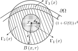
We use the following notations throughout this article. (1) Region $\Omega\subset\mathbb{R}^{3}$ is a unit-volume convex region, and $B(x,r)\subset\mathbb{R}^{3}$ is a ball centered at $x$ with radius $r$ . (2) Notation $|A|$ is a short for the volume of a measurable set $A\subset\mathbb{R}^{3}$ and $\|\cdot\|$ represents the length of a line segment. $\mathrm{Area}(\cdot)$ denotes the area of a surface. (3) $\mathrm{dist}(x,A)=\inf_{y\in A}\|xy\|$ where $x$ is a point and $A$ is a set. (4) Given any two nonnegative functions $f(n)$ and $g(n)$ , if there exist two constants $0<c_{1}<c_{2}$ such that $c_{1}g(n)\leq f(n)\leq c_{2}g(n)$ for any sufficiently large $n$ , then denote $f(n)=\Theta(g(n))$ . We also use notations $f(n)=o(g(n))$ and $f(n)\sim g(n)$ to denote that $\lim\limits_{n\rightarrow\infty}\frac{f(n)}{g(n)}=0$ and $\lim\limits_{n\rightarrow\infty}\frac{f(n)}{g(n)}=1$ , respectively. A surface is said to be smooth in this paper, meaning that its function has continuous second derivatives.

2 Proof of Proposition 1

Throughout this article, we define

\psi^{k}_{n,r}(x)=\frac{\left(n|B(x,r)\cap\Omega|\right)^{k}e^{-n|B(x,r)\cap\Omega|}}{k!}.

(7)

All left work in this section is to prove Proposition 1, i.e., $n\int_{\Omega}\psi^{k}_{n,r}(x)dx\sim e^{-c}.$ The proof will follow the framework proposed in [1] to carefully deal with the boundary of a convex region. The framework is developed based on the pioneering work of Wan et al. in [6] and [7], although in which only regular regions like disk or square are considered.

The following three conclusions are elementary, with their proof presented in Appendix A for reviewing.

Lemma 1.

Let $\Omega\subset\mathbb{R}^{3}$ be a bounded convex region, then there exists a positive constant $C$ such that for any sufficiently small $r$ , $\mathop{\inf}_{x\in\Omega}|B(x,r)\cap\Omega|\geq C\pi r^{3}.$ In particular, if $\partial\Omega$ is smooth, then $\forall x\in\partial\Omega$ , $\lim_{r\rightarrow 0}\frac{|B(x,r)\cap\Omega|}{\frac{4}{3}\pi r^{3}}=\frac{1}{2}$ .

Refer to caption — Figure 1: $\partial\Omega$ is tangent to $\gamma$ at point $O$

Lemma 2.

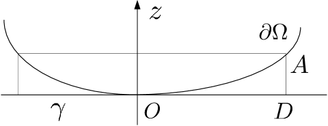
Suppose smooth surface $\partial\Omega$ is tangent to plane $\gamma$ at point $O$ , seeing Figure 1. Point $A\in\partial\Omega$ and $D\in\gamma$ , $AD\perp\gamma$ at point $D$ . Then

\|AD\|\leq G(\Omega)\|OD\|^{2}+o(\|OD\|),

(8)

where $G(\Omega)>0$ is a constant only depending on $\Omega$ . This leads to that if $\|AD\|>(G(\Omega)+1)r^{2}$ , then $\|OD\|>r,$ as long as $r$ is sufficiently small.

For any $t\in[0,r]$ , we define

a(r,t)=|\{x=(x_{1},x_{2},x_{3}):x_{1}^{2}+x_{2}^{2}+x_{3}^{2}\leq r^{2},x_{1}\leq t\}|.

(9)

$a(r,t)$ is usually shortly denoted by $a(t)$ . Here this definition follows the ones in [6, 7] where only the sets on planes are considered.

Lemma 3.

Let $r=r_{n}=\left(\frac{16}{5\pi}\frac{\log n+(\frac{3k}{2}-1)\log\log n+\xi}{n}\right)^{\frac{1}{3}}$ and $k\geq 1$ , then

n\int_{0}^{\frac{r}{2}}\frac{(na(t))^{k}e^{-na(t)}}{k!}dt\sim\frac{4}{3\pi}e^{-\frac{2\xi}{3}}\left(\frac{5\pi}{16}\right)^{\frac{2}{3}}\left(\frac{2}{3}\right)^{k}\frac{1}{k!}.

2.1 Case of smooth $\partial\Omega$

In this subsection, we assume the boundary $\partial\Omega$ be smooth. Let

\Omega(0)=\left\{x\in\Omega:\mathrm{dist}(x,\partial\Omega)\geq r\right\},\quad\Omega(2)=\left\{x\in\Omega:\mathrm{dist}(x,\partial\Omega)\leq(G(\Omega)+1)r^{2}\right\},

and define $\Omega(1)=\Omega\backslash\left(\Omega(0)\cup\Omega(2)\right).$ Here constant $G(\Omega)$ is given by Lemma 2, and $r$ is considered sufficiently small so that $\Omega(0)$ and $\Omega(2)$ are disjoint. Clearly,

\begin{split}&n\int_{\Omega}\psi^{k}_{n,r}(x)dx\mathrm{d}x=n\left(\int_{\Omega(0)}+\int_{\Omega(2)}+\int_{\Omega(1)}\right)\psi^{k}_{n,r}(x)dx\mathrm{d}x.\end{split}

Claim 1.

$n\int_{\Omega(0)}\psi^{k}_{n,r}(x)dx\sim o(1).$

Proof.

$\forall x\in\Omega(0),|B(x,r)\cap\Omega|=\frac{4}{3}\pi r^{3}$ . Notice that $|\Omega(0)|\sim(1-\mathrm{Area}(\Omega)r)$ .

\displaystyle n\int_{\Omega(0)}\psi^{k}_{n,r}(x)dx=\frac{n}{k!}\left(\frac{4n\pi r^{3}}{3}\right)^{k}e^{-\frac{4n\pi r^{3}}{3}}|\Omega(0)|\sim\frac{n}{k!}\left(\frac{4n\pi r^{3}}{3}\right)^{k}e^{-\frac{4n\pi r^{3}}{3}}=o(1).

∎

Claim 2.

$n\int_{\Omega(2)}\psi^{k}_{n,r}(x)dx=o(1).$

Proof.

Notice that $|\Omega(2)|\leq\mathrm{Area}(\Omega)\times(G(\Omega)+1)r^{2}=\Theta(1)r^{2}=\Theta\left(\left(\frac{\log n}{n}\right)^{\frac{2}{3}}\right)$ . By Lemma 1, there exists $r_{0}$ such that $\forall r<r_{0}$ , $|B(x,r)\cap\Omega|>\frac{1}{2}\pi r^{3}$ , which implies $\sup_{x\in\Omega(2)}e^{-n|B(x,r)\cap\Omega|}=o(n^{-1})$ .

\displaystyle n\int_{\Omega(2)}\psi^{k}_{n,r}(x)dx

\displaystyle\leq

\displaystyle\frac{n}{k!}(n\pi r^{3})^{k}[o(n^{-1})]|\Omega(2)|=o(1).

∎

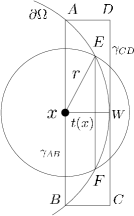
For any point $x\in\Omega(1)$ , let $W\in\partial\Omega$ be the nearest point to $x$ , i.e., $\|xW\|=\mathrm{dist}(x,\partial\Omega)<r.$ Let plane $\gamma_{CD}$ be tangent to $\partial\Omega$ at point $W$ , plane $\gamma_{AB}$ parallel $\gamma_{CD}$ and pass through point $x$ . Then $xW\bot\gamma_{CD}$ and $xW\bot\gamma_{AB}$ . See Figure 2(a). The distance between these two planes is $\|xW\|>(G(\Omega)+1)r^{2}$ , then by Lemma 2 we have that

\mathrm{dist}(x,\partial\Omega\cap\gamma_{AB})>r,

which implies that $\forall A\in\partial\Omega\cap\gamma_{AB}$ ,

\|xA\|>r.

The distance between point $x$ and point $y\in\partial\Omega$ is a continuous function of $y$ , which is due to the smooth boundary $\partial\Omega$ . By $\|xW\|<r$ and $\|xA\|>r$ , we know that any point $E^{\prime}\in\partial\Omega$ with $\|xE^{\prime}\|=r$ , or any point $E^{\prime}\in\partial\Omega\cap\partial B(x,r)$ , is between these two planes. Define

t(x,r)=\inf\{\mathrm{dist}(x,E^{\prime}F^{\prime})\mid E^{\prime},F^{\prime}\in\partial\Omega\cap\partial B(x,r)\},

then clearly $t(x,r)\geq 0$ . Here $t(x,r)$ is usually shortly denoted by $t(x)$ . Because $\partial\Omega\cap\partial B(x,r)$ is compact, we assume $E,F\in\partial\Omega\cap\partial B(x,r)$ such that

t(x,r)=\mathrm{dist}(x,EF)=\inf\{\mathrm{dist}(x,E^{\prime}F^{\prime})\mid E^{\prime},F^{\prime}\in\partial\Omega\cap\partial B(x,r)\}.

Furthermore, we set

\Omega(1,1)=\left\{x\in\Omega(1):t(x)\leq\frac{r}{2}\right\},\quad\Omega(1,2)=\Omega(1)\setminus\Omega(1,1).

In following, we will specify $n\int_{\Omega(1,2)}\psi^{k}_{n,r}(x)dx$ in Claim 3, and then determine $n\int_{\Omega(1,1)}\psi^{k}_{n,r}(x)dx$ in Claim 4. But at first, we will establish a lower and upper bounds for $|B(x,r)\cap\Omega|$ where $x\in\Omega(1)$ .

Because $t(x)>0$ , a lower bound is straightforward:

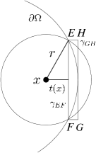
|B(x,r)\cap\Omega|\geq a(t(x))\geq\frac{2}{3}\pi r^{3}.

Now we give an upper bound for $|B(x,r)\cap\Omega|$ . Let $\gamma_{EF}$ be the plane passing through $EF$ with $\mathrm{dist}(x,\gamma_{EF})=t(x)$ . Plane $\gamma_{GH}$ parallels $\gamma_{EF}$ and tangents to $\partial\Omega$ . See Figure 2(b). Here we assume $EH\bot\gamma_{GH}$ and $FG\bot\gamma_{GH}$ .

Clearly $\|EF\|<2r$ , so

\mathrm{Area}(B(x,r)\cap\gamma_{EF})\leq\Theta(1)r^{2},

and by Lemma 2, $\|EH\|<\Theta(1)r^{2}$ . Therefore, the volume of cylinder $\mathrm{Cyc}(EFGH)$ which is formed by surface $B(x,r)\cap\gamma_{EF}$ and its projection on $\gamma_{FG}$ , satisfies

\mathrm{Vol}(\mathrm{Cyc}(EFGH))=\mathrm{Area}(B(x,r)\cap\gamma_{EF})\|EH\|\leq\Theta(1)r^{4}.

\displaystyle|B(x,r)\cap\Omega|\leq a(t(x))+\mathrm{Vol}(\mathrm{Cyc}(EFGH))\leq a(t(x))+\Theta(r^{4})\leq a(t(x))+\Theta(r^{4}).

With $a(t(x))\geq\frac{2\pi r^{3}}{3}$ that has been derived above, we obtain

\displaystyle|B(x,r)\cap\Omega|\leq a(t(x))\left(1+\frac{\Theta(r^{4})}{a(t(x))}\right)\leq a(t(x))(1+o(1)).

According to these lower and upper bounds of $|B(x,r)\cap\Omega|$ , we have the following estimates:

\begin{split}&(n|B(x,r)\cap\Omega|)^{k}e^{-n|B(x,r)\cap\Omega|}\leq(1+o(1))^{k}(na(t(x)))^{k}e^{-na(t(x))}.\end{split}

(10)

\begin{split}&(n|B(x,r)\cap\Omega|)^{k}e^{-n|B(x,r)\cap\Omega|}\geq(na(t(x)))^{k}e^{-n(a(t(x))+\Theta(r^{4}))}\geq e^{-n\Theta(r^{4})}(na(t(x)))^{k}e^{-na(t(x))}.\end{split}

(11)

Consider the integration on $\Omega(1,2)$ . Noticing that volume $|\Omega(1,2)|\leq\mathrm{Area}(\Omega)r$ and $\frac{2}{3}\pi r^{3}\leq a(t(x))\leq\frac{4}{3}\pi r^{3}$ , then by formula (10), we have

$\displaystyle n\int_{\Omega(1,2)}\psi^{k}_{n,r}(x)dx$	$\displaystyle=$	$\displaystyle\frac{n}{k!}\int_{\Omega(1,2)}\left(n\|B(x,r_{n})\cap\Omega\|\right)^{k}e^{-n\|B(x,r_{n})\cap\Omega\|}dx$
	$\displaystyle\leq$	$\displaystyle\frac{n}{k!}\left[(1+o(1))^{k}(na(t(x)))^{k}e^{-na(t(x))}\right]\|\Omega(1,2)\|$
	$\displaystyle\leq$	$\displaystyle\frac{n}{k!}(\frac{4}{3}n\pi r^{3})^{k}e^{-\frac{2}{3}n\pi r^{3}}\|\Omega(1,2)\|=o(1).$

This proves

Claim 3.

$n\int_{\Omega(1,2)}\psi^{k}_{n,r}(x)dx=o(1).$

In the following, we will determine $n\int_{\Omega(1,1)}\psi^{k}_{n,r}(x)dx$ . By estimates (10) and (11),

\displaystyle\frac{n}{k!}\int_{\Omega(1,1)}\left(n|B(x,r_{n})\cap\Omega|\right)^{k}e^{-n|B(x,r_{n})\cap\Omega|}dx\sim\frac{n}{k!}\int_{\Omega(1,1)}(na(t(x)))^{k}e^{-na(t(x))}dx.

We define

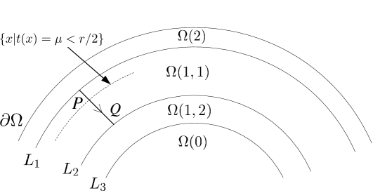
L_{1}=\{x\in\Omega\mid\mathrm{dist}(x,\partial\Omega)=(G(\Omega)+1)r^{2}\},\quad L_{2}=\{x\in\Omega(1)\mid t(x)=\frac{r}{2}\},

L_{3}=\{x\in\Omega\mid\mathrm{dist}(x,\partial\Omega)=r\}.

Clearly, the subregion $\Omega(1,1)$ has boundaries $L_{1}$ and $L_{2}$ , illustrated by Figure 2. If $x\in L_{1}$ , then $t(x)\geq 0$ by a similar argument as shown in the previous step. Clearly, $t(x)\leq(G(\Omega)+1)r^{2}$ . Therefore, $0\leq t(x)\leq(G(\Omega)+1)r^{2}$ for any $x\in L_{1}$ . As $r$ tends to zero, both surfaces $L_{1}$ and $L_{2}$ approximate the boundary $\partial\Omega$ . So there exists $\epsilon_{r}$ such that the area of $L_{1}$ and $L_{2}$ , denoted by $\mathrm{Area}(L_{1})$ and $\mathrm{Area}(L_{2})$ respectively, satisfies:

\mathrm{Area}(\partial\Omega)-\epsilon_{r}\leq\mathrm{Area}(L_{1}),\mathrm{Area}(L_{2})\leq\mathrm{Area}(\partial\Omega),

where $\epsilon_{r}\rightarrow 0$ as $r\rightarrow 0$ . In addition, it is clear that $t(x)$ is increasing along the directed line segment started from a point in $L_{1}$ to a point in $L_{2}$ . See the line segment $PQ$ in Figure 2.

The integration on $\Omega(1,1)$ can be bounded as follows:

\begin{split}&(\mathrm{Area}(\Omega)-\epsilon_{r})\frac{n}{k!}\int_{(G+1)r^{2}}^{\frac{r}{2}}(na(t))^{k}e^{-na(t)}dt\\ &\leq\frac{n}{k!}\int_{\Omega(1,1)}(na(t(x)))^{k}e^{-na(t(x))}dx\\ &\leq\mathrm{Area}(\Omega)\frac{n}{k!}\int_{0}^{\frac{r}{2}}(na(t))^{k}e^{-na(t)}dt.\end{split}

(12)

According to Lemma 3, we obtain that

\displaystyle\mathrm{Area}(\Omega)\frac{n}{k!}\int_{0}^{\frac{r}{2}}(na(t))^{k}e^{-na(t)}dt\sim\mathrm{Area}(\Omega)\frac{4}{3\pi}e^{-\frac{2\xi}{3}}\left(\frac{5\pi}{16}\right)^{\frac{2}{3}}\left(\frac{2}{3}\right)^{k}\frac{1}{k!}.

Therefore,

\begin{split}0&\leq\epsilon_{r}\int_{(G+1)r^{2}}^{\frac{r}{2}}\frac{n}{k!}(na(t))^{k}e^{-na(t)}dt\leq\epsilon_{r}\int_{0}^{\frac{r}{2}}\frac{n}{k!}(na(t))^{k}e^{-na(t)}dt=o(1).\end{split}

Furthermore, noticing that $2\pi r^{3}/3\leq a(t)\leq 2(\pi+\delta)r^{3}/3$ for any $t\in[0,(G(\Omega)+1)r^{2}]$ , where $\delta>0$ is a small real number, we have that

\mathrm{Area}(\Omega)\int_{0}^{(G+1)r^{2}}\frac{n}{k!}(na(t))^{k}e^{-na(t)}dt=o(1).

So,

\begin{split}&(\mathrm{Area}(\Omega)-\epsilon_{r})\frac{n}{k!}\int_{(G+1)r^{2}}^{\frac{r}{2}}(na(t))^{k}e^{-na(t)}dt\\ =&\frac{n}{k!}\left(\mathrm{Area}(\Omega)\int_{0}^{\frac{r}{2}}-\mathrm{Area}(\Omega)\int_{0}^{(G+1)r^{2}}-\epsilon_{r}\int_{(G+1)r^{2}}^{\frac{r}{2}}\right)(na(t))^{k}e^{-na(t)}dt\\ =&\mathrm{Area}(\Omega)\frac{n}{k!}\int_{0}^{\frac{r}{2}}(na(t))^{k}e^{-na(t)}dt+o(1).\end{split}

Then by formula (12),

			$\displaystyle\mathrm{Area}(\Omega)\frac{n}{k!}\int_{0}^{\frac{r}{2}}(na(t))^{k}e^{-na(t)}dt+o(1)$
		$\displaystyle=$	$\displaystyle(\mathrm{Area}(\Omega)-\epsilon_{r})\frac{n}{k!}\int_{(G+1)r^{2}}^{\frac{r}{2}}(na(t))^{k}e^{-na(t)}dt$
		$\displaystyle\leq$	$\displaystyle\frac{n}{k!}\int_{\Omega(1,1)}(na(t(x)))^{k}e^{-na(t(x))}dx$
		$\displaystyle\leq$	$\displaystyle\mathrm{Area}(\Omega)\frac{n}{k!}\int_{0}^{\frac{r}{2}}(na(t))^{k}e^{-na(t)}dt,$

which implies that

\displaystyle\frac{n}{k!}\int_{\Omega(1,1)}(na(t(x)))^{k}e^{-na(t(x))}dx\sim\mathrm{Area}(\Omega)\frac{n}{k!}\int_{0}^{\frac{r}{2}}(na(t))^{k}e^{-na(t)}dt.

So, by Lemma 3, we have

			$\displaystyle\frac{n}{k!}\int_{\Omega(1,1)}\left(n\|B(x,r_{n})\cap\Omega\|\right)^{k}e^{-n\|B(x,r_{n})\cap\Omega\|}dx$
		$\displaystyle\sim$	$\displaystyle\frac{n}{k!}\int_{\Omega(1,1)}(na(t(x)))^{k}e^{-na(t(x))}dx$
		$\displaystyle\sim$	$\displaystyle\mathrm{Area}(\Omega)\frac{n}{k!}\int_{0}^{\frac{r}{2}}(na(t))^{k}e^{-na(t)}dt$
		$\displaystyle\sim$	$\displaystyle\mathrm{Area}(\Omega)\frac{4}{3\pi}e^{-\frac{2\xi}{3}}\left(\frac{5\pi}{16}\right)^{\frac{2}{3}}\left(\frac{2}{3}\right)^{k}\frac{1}{k!}.$

Therefore, we have proved the following conclusion:

Claim 4.

$n\int_{\Omega(1,1)}\psi^{k}_{n,r}(x)dx\sim\mathrm{Area}(\Omega)\frac{4}{3\pi}e^{-\frac{2\xi}{3}}\left(\frac{5\pi}{16}\right)^{\frac{2}{3}}\left(\frac{2}{3}\right)^{k}\frac{1}{k!}.$

The four claims prove $\int_{\Omega}n\psi^{k}_{n,r}(x)dx=\left\{\int_{\Omega(0)}+\int_{\Omega(2)}+\int_{\Omega(1,2)}+\int_{\Omega(1,1)}\right\}n\psi^{k}_{n,r}(x)dx\sim e^{-c}.$

2.2 Case of continuous $\partial\Omega$

For a general unit-volume convex region $\Omega$ with a continuous rather than smooth boundary $\partial\Omega$ , we may use a family of convex regions $\{\Omega_{n}\}_{n=1}^{\infty}\subset\Omega$ to approximate $\Omega$ , where the boundary $\partial\Omega_{n}$ of each $\Omega_{n}$ is smooth. We set the width of the gap between $\partial\Omega$ and $\partial\Omega_{n}$ to be less than $r^{2}_{n}$ , That is, $\sup_{x\in\Omega_{n}}\mathrm{dist}(x,\partial\Omega)<r^{2}_{n}$ for any $n$ . Clearly, $\mathrm{Vol}(\Omega_{n})$ , the volume of $\Omega_{n}$ , satisfies $1-\mathrm{Area}(\Omega)r_{n}^{2}\leq\mathrm{Vol}(\Omega_{n})\leq 1.$ Because $\partial\Omega_{n}$ is smooth, follow the method presented in the previous subsection, we can also similarly obtain $n\int_{\Omega_{n}}\psi^{k}_{n,r}(x)dx\sim e^{-c}.$ Since the volume of $\Omega\setminus\Omega_{n}$ is no more than $\mathrm{Area}(\Omega)r_{n}^{2}$ , then by the proof of Claim 2, we have that $n\int_{\Omega\setminus\Omega_{n}}\psi^{k}_{n,r}(x)dx=o(1).$ Therefore,

n\int_{\Omega}\psi^{k}_{n,r}(x)dx=n\left(\int_{\Omega_{n}}+\int_{\Omega\setminus\Omega_{n}}\right)\psi^{k}_{n,r}(x)dx\sim e^{-c}.

This finally completes the proof of Proposition 1.

3 Proof of Proposition 2

We follow Penrose’s approach and framework to prove Proposition 2. For given $n$ , $x,y\in\Omega$ , let

v_{x}=|B(x,r)\cap\Omega|,v_{y}=|B(y,r)\cap\Omega|,v_{x,y}=|B(x,r)\cap B(y,r)\cap\Omega|,

v_{x\backslash y}=v_{x}-v_{x,y},v_{y\backslash x}=v_{y}-v_{x,y}.

Define $I_{i}=I_{i}(n)(i=1,2,3)$ as follows:

I_{1}=n^{2}\int_{\Omega}dx\int_{\Omega\cap B(x,3r)}dy\psi^{k}_{n,r}(y)\psi^{k}_{n,r}(x),

I_{2}=n^{2}\int_{\Omega}dx\int_{\Omega\cap B(x,r)}dy\Pr[Z_{1}+Z_{2}=Z_{1}+Z_{3}=k-1],

I_{3}=n^{2}\int_{\Omega}dx\int_{\Omega\cap B(x,3r)\backslash B(x,r)}dy\Pr[Z_{1}+Z_{2}=Z_{1}+Z_{3}=k],

where $Z_{1},Z_{2},Z_{3}$ are independent Poisson variables with means $nv_{x,y},nv_{x\backslash y},nv_{y\backslash x}$ respectively. As Penrose has pointed out in [5], by an argument similar to that of Section 7 of [8], to prove Proposition 2 it suffices to prove that $I_{1},I_{2},I_{3}\rightarrow 0$ as $n\rightarrow\infty$ . Firstly, we give the following conclusion.

Proposition 5.

Under the assumptions of Theorem 2, $Z_{3}$ is a Poisson variable with mean $nv_{y\backslash x}$ defined above, then

\frac{1}{n\pi r^{3}}\int_{\Omega}n\psi^{k}_{n,r}(x)dx\int_{\Omega\cap B(x,r)}n\Pr(Z_{3}=k-1)dy=o(1).

Proof.

The proof is shown in Appendix B. ∎

The conclusion of $I_{1},I_{2},I_{3}\rightarrow 0$ , as $n\rightarrow 0$ , will be proved by the following three claims.

Claim 5.

$I_{1}\rightarrow 0$ as $n\rightarrow\infty$ .

Proof.

By Lemma 1, there exists a constant $C>0$ such that $C\pi r^{3}\leq|B(x,r)\cap\Omega|\leq\frac{4}{3}\pi r^{3}$ .

$\displaystyle I_{1}$	$\displaystyle=$	$\displaystyle n^{2}\int_{\Omega}dx\int_{{\Omega}\cap B(x,3r)}dy\psi^{k}_{n,r}(y)\psi^{k}_{n,r}(x)$
	$\displaystyle=$	$\displaystyle\int_{\Omega}n\psi^{k}_{n,r}(x)dx\int_{B(x,3r)\cap\Omega}n\psi^{k}_{n,r}(y)dy$
	$\displaystyle\leq$	$\displaystyle\Theta(1)\int_{\Omega}n\psi^{k}_{n,r}(x)dx\int_{B(x,3r)\cap\Omega}\frac{1}{k!}n(n\pi r^{3})^{k}\exp(-Cn\pi r^{3})$
	$\displaystyle\leq$	$\displaystyle\Theta(1)\frac{n}{k!}\|B(x,3r)\|(n\pi r^{3})^{k}\exp(-Cn\pi r^{3})\int_{\Omega}n\psi^{k}_{n,r}(x)dx$
	$\displaystyle=$	$\displaystyle\Theta(1)(n\pi r^{3})^{k+1}\exp(-Cn\pi r^{3})\int_{\Omega}n\psi^{k}_{n,r}(x)dx$
	$\displaystyle\sim$	$\displaystyle\Theta(1)(n\pi r^{2})^{k+1}\exp(-Cn\pi r^{3})=o(1).$

∎

Claim 6.

$I_{2}\rightarrow 0$ , as $n\rightarrow\infty$ .

Proof.

It is obvious that $Z_{1}+Z_{2}$ and $Z_{3}$ are Possison variables with means $nv_{x}$ and $nv_{y\backslash x}$ respectively. Notice that

			$\displaystyle\Pr[Z_{1}+Z_{3}=k-1\|Z_{1}+Z_{2}=k-1]$
		$\displaystyle\leq$	$\displaystyle\sum_{j=0}^{k-1}\Pr[Z_{3}=k-1-j\|Z_{1}+Z_{2}=k-1]$
		$\displaystyle=$	$\displaystyle\sum_{j=0}^{k-1}\Pr[Z_{3}=k-1-j].$

For any $x\in\Omega$ , $\psi^{k}_{n,r}(x)=\frac{n|B(x,r)\cap\Omega|}{k}\psi^{k-1}_{n,r}(x),$ then by Lemma 1, there exists a constant $C>0$ such that $C\pi r^{3}\leq|B(x,r)\cap\Omega|$ , and thus $\psi^{k-1}_{n,r}(x)\leq\frac{k}{Cn\pi r^{3}}\psi^{k}_{n,r}(x).$ Therefore,

$\displaystyle I_{2}$	$\displaystyle=$	$\displaystyle n^{2}\int_{\Omega}dx\int_{\Omega\cap B(x,r)}dy\Pr[Z_{1}+Z_{2}=Z_{1}+Z_{3}=k-1]$
	$\displaystyle=$	$\displaystyle n^{2}\int_{\Omega}dx\int_{\Omega\cap B(x,r)}dy\Pr[Z_{1}+Z_{2}=k-1]\Pr[Z_{1}+Z_{3}=k-1\|Z_{1}+Z_{2}=k-1]$
	$\displaystyle=$	$\displaystyle n\int_{\Omega}\Pr[Z_{1}+Z_{2}=k-1]dx\int_{\Omega\cap B(x,r)}n\Pr[Z_{1}+Z_{3}=k-1\|Z_{1}+Z_{2}=k-1]dy$
	$\displaystyle\leq$	$\displaystyle n\int_{\Omega}\Pr[Z_{1}+Z_{2}=k-1]dx\left\{\sum_{j=0}^{k-1}\int_{\Omega\cap B(x,r)}n\Pr[Z_{3}=k-1-j]dy\right\}$
	$\displaystyle=$	$\displaystyle\sum_{j=0}^{k-1}\int_{\Omega}n\psi^{k-1}_{n,r}(x)dx\int_{\Omega\cap B(x,r)}n\Pr[Z_{3}=k-1-j]dy$
	$\displaystyle\leq$	$\displaystyle\frac{C}{k}\sum_{j=0}^{k-1}\frac{1}{n\pi r^{3}}\int_{\Omega}n\psi^{k}_{n,r}(x)dx\int_{\Omega\cap B(x,r)}n\Pr[Z_{3}=k-1-j]dy=o(1).$

The last equation holds due to Proposition 5 and the proved conclusion $\int_{\Omega}n\psi^{k}_{n,r}(x)dx\sim e^{-c}$ .

∎

Similarly, we can prove

Claim 7.

$I_{3}\rightarrow 0$ , as $n\rightarrow\infty$ .

Therefore, by these three claims, we know the Poissonized version (4) holds. The proof of Proposition 2 is completed.

4 Proofs of Proposition 3 and 4

Proposition 2 can lead to Proposition 3 by a de-Poissonized technique. The de-Poissonized technique is standard and thus omitted here, please see [5] for details.

Here we sketch the proof of Proposition 4. Penrose has clearly proved this result when region $\Omega$ is a square [5]. He constructed two events, $E_{n}(K)$ and $F_{n}(K)$ , such that for any $K>0$ ,

\left\{\rho(\chi_{n};\delta\geq k+1)\leq r_{n}<\rho(\chi_{n};\kappa\geq k+1)\right\}\subseteq E_{n}(K)\cup F_{n}(K),

and

\lim_{n\rightarrow\infty}\Pr[E_{n}(K)]=\lim_{n\rightarrow\infty}\Pr[F_{n}(K)]=0.

The definition of the events and the convergence results are organised in Proposition 5.1 and 5.2 of [5]. We do not introduce them in detail. Please refer to [5]. These conclusions can be straightly generalised to the case of convex region, with their proofs not much been modified. In fact, we have proved Proposition 1: $n\int_{\Omega}\psi^{k}_{n,r}(x)dx\sim e^{-c}$ , and $|B(x,r)\cap\Omega|$ in

\psi^{k}_{n,r}(x)=\frac{\left(n|B(x,r)\cap\Omega|\right)^{k}e^{-n|B(x,r)\cap\Omega|}}{k!}

can be bounded by $C\pi r^{3}\leq|B(x,r)\cap\Omega|\leq\frac{4}{3}\pi r^{3}$ where $C>0$ , seeing Lemma 1.

As a result, based on two generalised conclusions, a squeezing argument can lead to the following

\lim_{n\rightarrow\infty}\Pr\left\{\rho(\chi_{n};\delta\geq k+1)=\rho(\chi_{n};\kappa\geq k+1)\right\}=1.

Please see the details presented in [5].

References

[1] J. Ding, et. al., Asymptotic critical transmission radii in wireless networks over a convex region, submitted to IEEE Transactions on Information Theory (first round submission with Ref. IT-18-0767) (Nov. 2018).
[2] J. Ding, S. Ma, X. Zhu, Asymptotic critical transmission radii in wireless networks over a convex region, submitted to IEEE Transactions on Information Theory (second round submission with Ref. IT-21-0894) (Dec. 2021).
[3] H. Dette, N. Henze, The limit distribution of the largest nearest-neighbour link in the unit $d$ -cube, Journal of Applied Probability 26 (1) (1989) 67–80.
[4] M. D. Penrose, Random Geometric Graph, Oxford Univ. Press, 2003.
[5] M. D. Penrose, On $\kappa$ -connectivity for a geometric random graph, Random Struct. Algorithms 15 (1999) 145–164.
[6] P.-J. Wan, C.-W. Yi, Asymptotic critical transmission radius and critical neighbor number for $k$ -connectivity in wireless ad hoc networks, in: Proc. the 5th ACM international symposium on Mobile ad hoc networking and computing, 2004.
[7] P.-J. Wan, C.-W. Yi, L. Wang, Asymptotic critical transmission radius for $\kappa$ -connectivity in wireless ad hoc networks, IEEE Transactions on Information Theory 56 (6) (2010) 2867–2874.
[8] M. D. Penrose, The longest edge of the random minimal spanning tree, The Annals of Applied Probability 7 (2) (1997) 340–361.

Appendix A Proofs of Lemma 1, Lemma 2 and Lemma 3

The proofs of Lemma 1 and Lemma 2 are elementary and and similar to the ones presented in [1]. So they are omitted here. The following is the proof of Lemma 3.

Proof.

(Proof of Lemma 3). For convenience, we denote $C_{k}=\frac{3k}{2}-1$ . Notice that

a(t)=\frac{\pi}{3}(r-t)^{2}(2r+t),

a^{\prime}(t)=\pi(t^{2}-r^{2}),\quad a^{\prime\prime}(t)=2\pi t.

Let $f(t)=na(t)$ , then

n\int_{0}^{\frac{r}{2}}\frac{(f(t))^{k}e^{-f(t)}}{k!}dt=-\frac{1}{a^{\prime}(t)}e^{-f(t)}\sum_{k=0}^{k}\frac{(f(t))^{i}}{i!}|_{0}^{\frac{r}{2}}-\int_{0}^{\frac{r}{2}}\frac{a^{\prime\prime}(t)}{(a^{\prime}(t))^{2}}e^{-f(t)}\sum_{i=0}^{k}\frac{(f(t))^{i}}{i!}dt.

Notice that

f\left(\frac{r}{2}\right)=\frac{5n\pi r^{3}}{24}=\frac{5n\pi}{24}\frac{16}{5\pi}\frac{\log n+C_{k}\log\log n+\xi}{n}=\frac{2}{3}\left(\log n+C_{k}\log\log n+\xi\right).

e^{-f\left(\frac{r}{2}\right)}=\frac{1}{n^{\frac{2}{3}}}\frac{1}{(\log n)^{\frac{2}{3}C_{k}}}e^{-\frac{2\xi}{3}}.

(i) First term:

-\frac{1}{a^{\prime}\left(\frac{r}{2}\right)}e^{-f\left(\frac{r}{2}\right)}=\frac{1}{\frac{3}{4}\pi r^{2}}\frac{1}{n^{\frac{2}{3}}}\frac{1}{(\log n)^{\frac{2}{3}}}e^{-\frac{2\xi}{3}}=\frac{4}{3\pi}e^{-\frac{2\xi}{3}}\frac{\left(\frac{5\pi}{16}\frac{n}{\log n+C_{k}\log\log n}\right)^{\frac{2}{3}}}{n^{\frac{2}{3}}(\log n)^{\frac{2}{3}C_{k}}}

-\frac{1}{a^{\prime}\left(\frac{r}{2}\right)}e^{-f\left(\frac{r}{2}\right)}\sum_{i=0}^{k}\frac{f\left(\frac{r}{2}\right)^{i}}{i!}=\frac{4}{3\pi}e^{-\frac{2\xi}{3}}\frac{\left(\frac{5\pi}{16}\frac{n}{\log n+C_{k}\log\log n+\xi}\right)^{\frac{2}{3}}}{n^{\frac{2}{3}}(\log n)^{\frac{2}{3}C_{k}}}\sum_{i=0}^{k}\left(\frac{2}{3}\left(\log n+C_{k}\log\log n+\xi\right)\right)^{i}/i!

Because $C_{k}=\frac{3}{2}k-1$ , so $\left(\log n\right)^{\frac{2}{3}+\frac{2}{3}C_{k}}=\left(\log n\right)^{k}$ , and

-\frac{1}{a^{\prime}\left(\frac{r}{2}\right)}e^{-f\left(\frac{r}{2}\right)}\sum_{i=0}^{k}\frac{f\left(\frac{r}{2}\right)^{i}}{i!}\sim-\frac{1}{a^{\prime}\left(\frac{r}{2}\right)}e^{-f\left(\frac{r}{2}\right)}\frac{f\left(\frac{r}{2}\right)^{k}}{k!}\sim\frac{4}{3\pi}e^{-\frac{2\xi}{3}}\left(\frac{5\pi}{16}\right)^{\frac{2}{3}}\left(\frac{2}{3}\right)^{k}\frac{1}{k!}.

(ii) Second term. Notice that

a^{\prime}(0)=-\pi r^{2},\quad f\left(0\right)=\frac{32}{15}\left(\log n+C_{k}\log\log n+\xi\right),\quad e^{-f(0)}=\frac{1}{n^{\frac{32}{15}}}\frac{1}{(\log n)^{\frac{32}{15}C_{k}}}e^{-\frac{32\xi}{15}}.

It is easy to see that

-\frac{1}{a^{\prime}\left(0\right)}e^{-f\left(0\right)}f\left(0\right)^{k}=o(1).

(iii) Third term.

a^{\prime}(t)=\pi(t^{2}-r^{2}),\quad a^{\prime\prime}(t)=2\pi t,

When $t\leq\frac{r}{2}$ ,

\left|\frac{a^{\prime\prime}(t)}{(a^{\prime}(t))^{3}}\right|=\frac{2}{\pi^{2}}\frac{t}{(r^{2}-t^{2})^{3}}\leq\frac{64}{27\pi^{2}}\frac{1}{r^{5}}=\Theta\left(\left(\frac{n}{\log n+C_{k}\log\log n+\xi}\right)^{\frac{5}{3}}\right).

Then

			$\displaystyle\left\|\int_{0}^{\frac{r}{2}}\frac{a^{\prime\prime}(t)}{(a^{\prime}(t))^{2}}e^{-f(t)}\sum_{i=0}^{k}\frac{(f(t))^{i}}{i!}dt\right\|$
		$\displaystyle=$	$\displaystyle\frac{1}{n}\left\|\int_{0}^{\frac{r}{2}}\frac{a^{\prime\prime}(t)}{(a^{\prime}(t))^{3}}e^{-f(t)}\sum_{i=0}^{k}\frac{(f(t))^{i}}{i!}df(t)\right\|$
		$\displaystyle\leq$	$\displaystyle\frac{64}{27\pi^{2}}\frac{1}{nr^{5}}\left\|\int_{0}^{\frac{r}{2}}e^{-f(t)}\sum_{i=0}^{k}\frac{(f(t))^{i}}{i!}df(t)\right\|$
		$\displaystyle\leq$	$\displaystyle\Theta(1)\frac{64}{27\pi^{2}}\frac{1}{nr^{5}}\left\|\int_{0}^{\frac{r}{2}}e^{-f(t)}\frac{(f(t))^{k}}{k!}df(t)\right\|$
		$\displaystyle=$	$\displaystyle\Theta(1)\frac{64}{27\pi^{2}}\frac{1}{nr^{5}}\left\|\int_{0}^{\frac{r}{2}}d\left(-e^{-f(t)}\sum_{i=0}^{k}\frac{(f(t))^{i}}{i!}\right)\right\|$
		$\displaystyle\leq$	$\displaystyle\Theta(1)\frac{64}{27\pi^{2}}\frac{1}{nr^{5}}e^{-f(0)}\sum_{i=0}^{k}\frac{(f(0))^{i}}{i!}$
		$\displaystyle=$	$\displaystyle o(1).$

Therefore,

n\int_{0}^{\frac{r}{2}}\frac{(f(t))^{k}e^{-f(t)}}{k!}dt\sim-\frac{1}{a^{\prime}\left(\frac{r}{2}\right)}e^{-f\left(\frac{r}{2}\right)}\frac{f\left(\frac{r}{2}\right)^{k}}{k!}\sim\frac{4}{3\pi}e^{-\frac{2\xi}{3}}\left(\frac{5\pi}{16}\right)^{\frac{2}{3}}\left(\frac{2}{3}\right)^{k}\frac{1}{k!}.

∎

Appendix B Proof of Proposition 5

We first give a lemma.

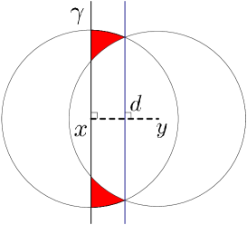
Lemma 4.

The distance between the centers $x$ and $y$ of two balls which have the same radium $r$ is less than the radius, i.e., $d=\|xy\|<r$ . Plane $\gamma$ is perpendicular to line $xy$ and passes through point $x$ . The semi-sphere cut by $\gamma$ which contains point $y$ is denoted by $B_{\mathrm{semi}}(x,r)$ , then the volume of $B_{\mathrm{semi}}(x,r)\setminus B(y,r)$ (see red part in Figure 3) is

V^{*}(d)=|B_{\mathrm{semi}}\setminus B(y,r)|=\frac{1}{4}\pi d^{3}.

Proof.

$V^{*}(d)=\int_{0}^{\frac{d}{2}}\pi\left((r^{2}-t^{2})-(r^{2}-(d-t)^{2})\right)dt=\frac{1}{4}\pi d^{3}.$ ∎

Proof.

(Proof for Proposition 5). Let $d_{0}=\left(\frac{4r}{n^{\frac{2}{3}}\pi^{\frac{2}{3}}}\right)^{\frac{1}{3}},$ then $0<d_{0}=\Theta\left(\frac{(\log n)^{\frac{1}{9}}}{n^{\frac{1}{3}}}\right)<r$ for any sufficiently large $n$ , and $\frac{n\pi d_{0}^{3}}{4}=(n\pi r^{3})^{\frac{1}{3}}.$ $\forall x\in\Omega$ , let

\Gamma_{1}(x)=\left\{y\in B(x,r)\cap\Omega:\mathrm{dist}(y,x)\leq d_{0}\right\},

\Gamma_{2}(x)=\left\{y\in B(x,r)\cap\Omega:\mathrm{dist}(y,x)\geq d_{0},\mathrm{dist}(y,\partial\Omega)>(G(\Omega)+1)r^{2}\right\},

\Gamma_{3}(x)=\left\{y\in B(x,r)\cap\Omega:\mathrm{dist}(y,\partial\Omega)\leq(G(\Omega)+1)r^{2}\right\}.

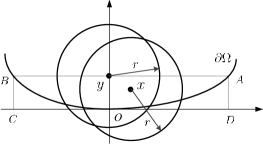
Here $\mathrm{dist}(y,x)=\|yx\|$ , the distance between points $y$ and $x$ . Constant $G(\Omega)$ is an uniform upper bound given in Lemma 2. Clearly, $B(x,r)\cap\Omega\subset\Gamma_{1}(x)\cup\Gamma_{2}(x)\cup\Gamma_{3}(x),$ as Figure 4(a) illustrates.

Let

A_{i}=\frac{1}{n\pi r^{3}}\int_{\Omega}n\psi^{k}_{n,r}(x)dx\int_{\Gamma_{i}(x)}n\Pr(Z_{3}=k-1)dy,i=1,2,3.

(13)

We will prove $A_{i}=o(1),i=1,2,3$ , in the following three steps. Notice that we have proved Proposition 1: $\int_{\Omega}n\psi^{k}_{n,r}(x)dx\sim e^{-c}$ .

Step 1: to prove $A_{1}=o(1)$ .

$\displaystyle A_{1}$	$\displaystyle=$	$\displaystyle\frac{1}{n\pi r^{3}}\int_{\Omega}n\psi^{k}_{n,r}(x)dx\int_{\Gamma_{1}(x)}n\Pr(Z_{3}=k-1)dy$
	$\displaystyle\leq$	$\displaystyle\frac{1}{n\pi r^{3}}\int_{\Omega}n\psi^{k}_{n,r}(x)dx\int_{\Gamma_{1}(x)}ndy$
	$\displaystyle\leq$	$\displaystyle\frac{1}{\pi r^{3}}\int_{\Omega}\|\Gamma_{1}(x)\|n\psi^{k}_{n,r}(x)dx$
	$\displaystyle\leq$	$\displaystyle\Theta(1)\frac{d_{0}^{3}}{r^{3}}\int_{\Omega}n\psi^{k}_{n,r}(x)dx=o(1).$

Step 2: to prove $A_{2}=o(1)$ . For any $y\in\Gamma_{2}(x)$ , $\mathrm{dist}(y,\partial\Omega)\geq(G(\Omega)+1)r^{2}$ . Then by Lemma 2, $\|yA\|>r$ and $\|yB\|>r$ , see Figure 4(b). This means that at least more than one half of $B(y,r)$ falling in $\Omega$ . As a result,

v_{y\backslash x}=|B(y,r)\cap\Omega|-|B(x,r)\cap B(y,r)\cap\Omega|\geq\frac{V^{\ast}(d_{0})}{2},

where $V^{\ast}(d_{0})$ is given by Lemma 4. Therefore, $nv_{y\backslash x}\geq\frac{1}{2}nV^{\ast}(d_{0})=\frac{n}{2}\frac{\pi d_{0}^{3}}{4}=\frac{1}{2}(n\pi r^{3})^{\frac{1}{3}}.$

$\displaystyle A_{2}$	$\displaystyle=$	$\displaystyle\frac{1}{n\pi r^{3}}\int_{\Omega}n\psi^{k}_{n,r}(x)dx\int_{\Gamma_{2}}n\Pr(Z_{3}=k-1)dy$
	$\displaystyle\leq$	$\displaystyle\frac{1}{n\pi r^{3}}\int_{\Omega}n\psi^{k}_{n,r}(x)dx\int_{\Gamma_{2}}\frac{n(n\pi r^{3})^{k-1}\exp\left(-\frac{1}{2}\left(n\pi r^{3}\right)^{\frac{1}{3}}\right)dy}{(k-1)!}$
	$\displaystyle\leq$	$\displaystyle\frac{1}{n\pi r^{3}}\int_{\Omega}n\psi^{k}_{n,r}(x)dx\frac{(n\pi r^{3})^{k}\exp\left(-\frac{1}{2}\left(n\pi r^{3}\right)^{\frac{1}{3}}\right)}{(k-1)!}$
	$\displaystyle\sim$	$\displaystyle\frac{e^{-c}}{n\pi r^{3}}o(1)=o(1).$

Step 3: to prove $A_{3}=o(1)$ . Notice that $\Gamma_{3}(x)$ falls in a region with the width less than $(G(\Omega)+1)r^{2}$ , we have $|\Gamma_{3}(x)|\leq\mathrm{Area}(\partial B(x,r))(G(\Omega)+1)r^{2}=\Theta(1)r^{4}.$

$\displaystyle A_{3}$	$\displaystyle=$	$\displaystyle\frac{1}{n\pi r^{3}}\int_{\Omega}n\psi^{k}_{n,r}(x)dx\int_{\Gamma_{3}(x)}n\Pr(Z_{3}=k-1)dy$
	$\displaystyle\leq$	$\displaystyle\frac{1}{n\pi r^{3}}\int_{\Omega}n\psi^{k}_{n,r}(x)dx\int_{\Gamma_{3}(x)}ndy$
	$\displaystyle=$	$\displaystyle\frac{1}{\pi r^{3}}\int_{\Omega}\|\Gamma_{3}(x)\|n\psi^{k}_{n,r}(x)dx$
	$\displaystyle\leq$	$\displaystyle\Theta(r)\int_{\Omega}n\psi^{k}_{n,r}(x)dx=o(1).$

Finally, we have

\frac{1}{n\pi r^{3}}\int_{\Omega}n\psi^{k}_{n,r}(x)dx\int_{\Omega\cap B(x,r)}n\Pr(Z_{3}=k-1)dy\leq A_{1}+A_{2}+A_{3}=o(1).

The proposition is therefore proved. ∎

Asymptotic Critical Radii in Random Geometric Graphs over 3-Dimensional Convex regions

Abstract

keywords:

1 Introduction and main results

Theorem 1.

Theorem 2.

Proposition 1.

Proposition 2.

Proposition 3.

Proposition 4.

2 Proof of Proposition 1

Lemma 1.

Lemma 2.

Lemma 3.

2.1 Case of smooth ∂Ω\partial\Omega

Claim 1.

Proof.

Claim 2.

Proof.

Claim 3.

Claim 4.

2.2 Case of continuous ∂Ω\partial\Omega

3 Proof of Proposition 2

Proposition 5.

Proof.

Claim 5.

Proof.

Claim 6.

Proof.

Claim 7.

4 Proofs of Proposition 3 and 4

References

References

Appendix A Proofs of Lemma 1, Lemma 2 and Lemma 3

Proof.

Appendix B Proof of Proposition 5

Lemma 4.

Proof.

Proof.

2.1 Case of smooth $\partial\Omega$

2.2 Case of continuous $\partial\Omega$