Asymptotic Distribution of the Markowitz Portfolio

Abstract

The asymptotic distribution of the Markowitz portfolio, ${{\mathsf{\hat{\Sigma}}}^{-1}}{\boldsymbol{\hat{\mu}}}$ , is derived, for the general case (assuming fourth moments of returns exist), and for the case of multivariate normal returns. The derivation allows for inference which is robust to heteroskedasticity and autocorrelation of moments up to order four. As a side effect, one can estimate the proportion of error in the Markowitz portfolio due to mis-estimation of the covariance matrix. A likelihood ratio test is given which generalizes Dempster’s Covariance Selection test to allow inference on linear combinations of the precision matrix and the Markowitz portfolio. [15] Extensions of the main method to deal with hedged portfolios, conditional heteroskedasticity, conditional expectation, and constrained estimation are given. It is shown that the Hotelling-Lawley statistic generalizes the (squared) Sharpe ratio under the conditional expectation model. Asymptotic distributions of all four of the common ‘MGLH’ statistics are found, assuming random covariates. [60] Examples are given demonstrating the possible uses of these results.

1 Introduction

Given $p$ assets with expected return $\boldsymbol{\mu}$ and covariance of return $\mathsf{\Sigma}$ , the portfolio defined as

{\boldsymbol{\nu}}_{{}*}=_{\operatorname{df}}\lambda{{\mathsf{\Sigma}}^{-1}}{\boldsymbol{\mu}}

(1)

plays a special role in modern portfolio theory. [38, 5, 9] It is known as the ‘efficient portfolio’, the ‘tangency portfolio’, and, somewhat informally, the ‘Markowitz portfolio’. It appears, for various $\lambda$ , in the solution to numerous portfolio optimization problems. Besides the classic mean-variance formulation, it solves the (population) Sharpe ratio maximization problem:

\max_{\boldsymbol{\nu}:{{\boldsymbol{\nu}}^{\top}}\mathsf{\Sigma}\boldsymbol{\nu}\leq R^{2}}\frac{{{\boldsymbol{\nu}}^{\top}}\boldsymbol{\mu}-{{r}_{0}}}{\sqrt{{{\boldsymbol{\nu}}^{\top}}\mathsf{\Sigma}\boldsymbol{\nu}}},

(2)

where ${{r}_{0}}\geq 0$ is the risk-free, or ‘disastrous’, rate of return, and $R>0$ is some given ‘risk budget’. The solution to this optimization problem is $\lambda{{\mathsf{\Sigma}}^{-1}}{\boldsymbol{\mu}}$ , where $\lambda=R/\sqrt{{{\boldsymbol{\mu}}^{\top}}{{\mathsf{\Sigma}}^{-1}}\boldsymbol{\mu}}.$

In practice, the Markowitz portfolio has a somewhat checkered history. The population parameters $\boldsymbol{\mu}$ and $\mathsf{\Sigma}$ are not known and must be estimated from samples. Estimation error results in a feasible portfolio, ${\boldsymbol{\hat{\nu}}}_{{}*}$ , of dubious value. Michaud went so far as to call mean-variance optimization, “error maximization.” [44] It has been suggested that simple portfolio heuristics outperform the Markowitz portfolio in practice. [13]

This paper focuses on the asymptotic distribution of the sample Markowitz portfolio. By formulating the problem as a linear regression, Britten-Jones very cleverly devised hypothesis tests on elements of ${\boldsymbol{\nu}}_{{}*}$ , assuming multivariate Gaussian returns. [7] In a remarkable series of papers, Okhrin and Schmid, and Bodnar and Okhrin give the (univariate) density of the dot product of ${\boldsymbol{\nu}}_{{}*}$ and a deterministic vector, again for the case of Gaussian returns. [50, 3] Okhrin and Schmid also show that all moments of ${\boldsymbol{\hat{\nu}}}_{{}*}/{{\boldsymbol{1}}^{\top}}{\boldsymbol{\hat{\nu}}}_{{}*}$ of order greater than or equal to one do not exist. [50]

Here I derive asymptotic normality of ${\boldsymbol{\hat{\nu}}}_{{}*}$ , the sample analogue of ${\boldsymbol{\nu}}_{{}*}$ , assuming only that the first four moments exist. Feasible estimation of the variance of ${\boldsymbol{\hat{\nu}}}_{{}*}$ is amenable to heteroskedasticity and autocorrelation robust inference. [68] The asymptotic distribution under Gaussian returns is also derived.

After estimating the covariance of ${\boldsymbol{\hat{\nu}}}_{{}*}$ , one can compute Wald test statistics for the elements of ${\boldsymbol{\hat{\nu}}}_{{}*}$ , possibly leading one to drop some assets from consideration (‘sparsification’). Having an estimate of the covariance can also allow portfolio shrinkage. [14, 31]

The derivations in this paper actually solve a more general problem than the distribution of the sample Markowitz portfolio. The covariance of ${\boldsymbol{\hat{\nu}}}_{{}*}$ and the ‘precision matrix,’ ${{\mathsf{\hat{\Sigma}}}^{-1}}$ are derived. This allows one, for example, to estimate the proportion of error in the Markowitz portfolio attributable to mis-estimation of the covariance matrix. According to lore, the error in portfolio weights is mostly attributable to mis-estimation of $\boldsymbol{\mu}$ , not of $\mathsf{\Sigma}$ . [8, 43]

Finally, assuming Gaussian returns, a likelihood ratio test for performing inference on linear combinations of elements of the Markowitz portfolio and the precision matrix is derived. This test generalizes a procedure by Dempster for inference on the precision matrix alone. [15]

2 The augmented second moment

Let $\boldsymbol{x}$ be an array of returns of $p$ assets, with mean $\boldsymbol{\mu}$ , and covariance $\mathsf{\Sigma}$ . Let $\boldsymbol{\tilde{x}}$ be $\boldsymbol{x}$ prepended with a 1: $\boldsymbol{\tilde{x}}={{\left[1,{{\boldsymbol{x}}^{\top}}\right]}^{\top}}$ . Consider the second moment of $\boldsymbol{\tilde{x}}$ :

\mathsf{\Theta}=_{\operatorname{df}}\operatorname{E}\left[\boldsymbol{\tilde{x}}{{\boldsymbol{\tilde{x}}}^{\top}}\right]=\left[\begin{array}[]{cc}{1}&{{{\boldsymbol{\mu}}^{\top}}}\\ {\boldsymbol{\mu}}&{\mathsf{\Sigma}+\boldsymbol{\mu}{{\boldsymbol{\mu}}^{\top}}}\end{array}\right].

(3)

By inspection one can confirm that the inverse of $\mathsf{\Theta}$ is

{{\mathsf{\Theta}}^{-1}}=\left[\begin{array}[]{cc}{1+{{\boldsymbol{\mu}}^{\top}}{{\mathsf{\Sigma}}^{-1}}\boldsymbol{\mu}}&{-{{\boldsymbol{\mu}}^{\top}}{{\mathsf{\Sigma}}^{-1}}}\\ {-{{\mathsf{\Sigma}}^{-1}}\boldsymbol{\mu}}&{{{\mathsf{\Sigma}}^{-1}}}\end{array}\right]=\left[\begin{array}[]{cc}{1+{\zeta}^{2}_{*}}&{-{{{\boldsymbol{\nu}}_{{}*}}^{\top}}}\\ {-{\boldsymbol{\nu}}_{{}*}}&{{{\mathsf{\Sigma}}^{-1}}}\end{array}\right],

(4)

where ${\boldsymbol{\nu}}_{{}*}={{\mathsf{\Sigma}}^{-1}}{\boldsymbol{\hat{\mu}}}$ is the Markowitz portfolio, and ${\zeta}_{*}=\sqrt{{{\boldsymbol{\mu}}^{\top}}{{\mathsf{\Sigma}}^{-1}}\boldsymbol{\mu}}$ is the Sharpe ratio of that portfolio. The matrix $\mathsf{\Theta}$ contains the first and second moment of $\boldsymbol{x}$ , but is also the uncentered second moment of $\boldsymbol{\tilde{x}}$ , a fact which makes it amenable to analysis via the central limit theorem.

The relationships above are merely facts of linear algebra, and so hold for sample estimates as well:

{{\left[\begin{array}[]{cc}{1}&{{{\boldsymbol{\hat{\mu}}}^{\top}}}\\ {\boldsymbol{\hat{\mu}}}&{\mathsf{\hat{\Sigma}}+\boldsymbol{\hat{\mu}}{{\boldsymbol{\hat{\mu}}}^{\top}}}\end{array}\right]}^{-1}}={\left[\begin{array}[]{cc}{1+{\hat{\zeta}}^{2}_{*}}&{-{{{\boldsymbol{\hat{\nu}}}_{{}*}}^{\top}}}\\ {-{\boldsymbol{\hat{\nu}}}_{{}*}}&{{{\mathsf{\hat{\Sigma}}}^{-1}}}\end{array}\right]},

where $\boldsymbol{\hat{\mu}}$ , $\mathsf{\hat{\Sigma}}$ are some sample estimates of $\boldsymbol{\mu}$ and $\mathsf{\Sigma}$ , and ${\boldsymbol{\hat{\nu}}}_{{}*}={{\mathsf{\hat{\Sigma}}}^{-1}}{\boldsymbol{\hat{\mu}}},{\hat{\zeta}}^{2}_{*}={{\boldsymbol{\hat{\mu}}}^{\top}}{{\mathsf{\hat{\Sigma}}}^{-1}}\boldsymbol{\hat{\mu}}$ .

Given $n$ i.i.d. observations ${\boldsymbol{x}}_{i}$ , let $\mathsf{\tilde{{X}}}$ be the matrix whose rows are the vectors ${{{\boldsymbol{\tilde{x}}}_{i}}^{\top}}$ . The naïve sample estimator

\mathsf{\hat{\Theta}}=_{\operatorname{df}}\frac{1}{n}{{\mathsf{\tilde{{X}}}}^{\top}}\mathsf{\tilde{{X}}}

(5)

is an unbiased estimator since $\mathsf{\Theta}=\operatorname{E}\left[{{\boldsymbol{\tilde{x}}}^{\top}}\boldsymbol{\tilde{x}}\right]$ .

2.1 Matrix Derivatives

Some notation and technical results concerning matrices are required.

Definition 2.1 (Matrix operations).

For matrix $\mathsf{A}$ , let $\operatorname{vec}\left(\mathsf{A}\right)$ , and $\operatorname{vech}\left(\mathsf{A}\right)$ be the vector and half-space vector operators. The former turns an ${p}\times{p}$ matrix into an $p^{2}$ vector of its columns stacked on top of each other; the latter vectorizes a symmetric (or lower triangular) matrix into a vector of the non-redundant elements. Let $\mathsf{L}$ be the ‘Elimination Matrix,’ a matrix of zeros and ones with the property that $\operatorname{vech}\left(\mathsf{A}\right)=\mathsf{L}\operatorname{vec}\left(\mathsf{A}\right).$ The ‘Duplication Matrix,’ $\mathsf{D}$ , is the matrix of zeros and ones that reverses this operation: $\mathsf{D}\operatorname{vech}\left(\mathsf{A}\right)=\operatorname{vec}\left(\mathsf{A}\right).$ [36] Note that this implies that

\mathsf{L}\mathsf{D}=\mathsf{I}\left(\neq\mathsf{D}\mathsf{L}\right).

We will let $\mathsf{K}$ be the ’commutation matrix’, i.e., the matrix whose rows are a permutation of the rows of the identity matrix such that $\mathsf{K}\operatorname{vec}\left(\mathsf{A}\right)=\operatorname{vec}\left({{\mathsf{A}}^{\top}}\right)$ for square matrix $\mathsf{A}$ .

Definition 2.2 (Derivatives).

For $m$ -vector $\boldsymbol{x}$ , and $n$ -vector $\boldsymbol{y}$ , let the derivative $\frac{\mathrm{d}{\boldsymbol{y}}}{\mathrm{d}\boldsymbol{x}}$ be the ${n}\times{m}$ matrix whose first column is the partial derivative of $\boldsymbol{y}$ with respect to $x_{1}$ . This follows the so-called ‘numerator layout’ convention. For matrices $\mathsf{Y}$ and $\mathsf{X}$ , define

\frac{\mathrm{d}{\mathsf{Y}}}{\mathrm{d}\mathsf{X}}=_{\operatorname{df}}\frac{\mathrm{d}{\operatorname{vec}\left(\mathsf{Y}\right)}}{\mathrm{d}\operatorname{vec}\left(\mathsf{X}\right)}.

Lemma 2.3 (Miscellaneous Derivatives).

For symmetric matrices $\mathsf{Y}$ and $\mathsf{X}$ ,

\frac{\mathrm{d}{\operatorname{vech}\left(\mathsf{Y}\right)}}{\mathrm{d}\operatorname{vec}\left(\mathsf{X}\right)}=\mathsf{L}\frac{\mathrm{d}{\mathsf{Y}}}{\mathrm{d}\mathsf{X}},\quad\frac{\mathrm{d}{\operatorname{vec}\left(\mathsf{Y}\right)}}{\mathrm{d}\operatorname{vech}\left(\mathsf{X}\right)}=\frac{\mathrm{d}{\mathsf{Y}}}{\mathrm{d}\mathsf{X}}\mathsf{D},\quad\frac{\mathrm{d}{\operatorname{vech}\left(\mathsf{Y}\right)}}{\mathrm{d}\operatorname{vech}\left(\mathsf{X}\right)}=\mathsf{L}{\frac{\mathrm{d}{\mathsf{Y}}}{\mathrm{d}\mathsf{X}}}\mathsf{D}.

(6)

Proof.

For the first equation, note that $\operatorname{vech}\left(\mathsf{Y}\right)=\mathsf{L}\operatorname{vec}\left(\mathsf{Y}\right)$ , thus by the chain rule:

\frac{\mathrm{d}{\operatorname{vech}\left(\mathsf{Y}\right)}}{\mathrm{d}\operatorname{vec}\left(\mathsf{X}\right)}=\frac{\mathrm{d}{\mathsf{L}\operatorname{vec}\left(\mathsf{Y}\right)}}{\mathrm{d}\operatorname{vec}\left(\mathsf{Y}\right)}=\mathsf{L}\frac{\mathrm{d}{\mathsf{Y}}}{\mathrm{d}\mathsf{X}},

by linearity of the derivative. The other identities follow similarly. ∎

Lemma 2.4 (Derivative of matrix inverse).

For invertible matrix $\mathsf{A}$ ,

\frac{\mathrm{d}{{{\mathsf{A}}^{-1}}}}{\mathrm{d}\mathsf{A}}=-\left({{\mathsf{A}}^{-\top}}\otimes{{\mathsf{A}}^{-1}}\right)=-{{\left({{\mathsf{A}}^{\top}}\otimes\mathsf{A}\right)}^{-1}}.

(7)

For symmetric $\mathsf{A}$ , the derivative with respect to the non-redundant part is

\frac{\mathrm{d}{\operatorname{vech}\left({{\mathsf{A}}^{-1}}\right)}}{\mathrm{d}\operatorname{vech}\left(\mathsf{A}\right)}=-\mathsf{L}{\left({{\mathsf{A}}^{-1}}\otimes{{\mathsf{A}}^{-1}}\right)}\mathsf{D}.

(8)

Note how this result generalizes the scalar derivative: $\frac{\mathrm{d}{x^{-1}}}{\mathrm{d}x}=-\left(x^{-1}x^{-1}\right).$

Proof.

Equation 7 is a known result. [18, 37] Equation 8 then follows using Lemma 2.3. ∎

2.2 Asymptotic distribution of the Markowitz portfolio

Collecting the mean and covariance into the second moment matrix gives the asymptotic distribution of the sample Markowitz portfolio without much work. In some sense, this computation generalizes the ‘standard’ asymptotic analysis of Sharpe ratio of multiple assets. [27, 34, 32, 33]

Theorem 2.5.

Let $\mathsf{\hat{\Theta}}$ be the unbiased sample estimate of $\mathsf{\Theta}$ , based on $n$ i.i.d. samples of $\boldsymbol{x}$ . Let $\mathsf{\Omega}$ be the variance of $\operatorname{vech}\left(\boldsymbol{\tilde{x}}{{\boldsymbol{\tilde{x}}}^{\top}}\right)$ . Then, asymptotically in $n$ ,

\sqrt{n}\left(\operatorname{vech}\left({{\mathsf{\hat{\Theta}}}^{-1}}\right)-\operatorname{vech}\left({{\mathsf{\Theta}}^{-1}}\right)\right)\rightsquigarrow\mathcal{N}\left(0,\mathsf{H}\mathsf{\Omega}{{\mathsf{H}}^{\top}}\right),

(9)

where

\mathsf{H}=-\mathsf{L}{\left({{{\mathsf{\Theta}}^{-1}}}\otimes{{{\mathsf{\Theta}}^{-1}}}\right)}\mathsf{D}.

(10)

Furthermore, we may replace $\mathsf{\Omega}$ in this equation with an asymptotically consistent estimator, $\mathsf{\hat{\Omega}}$ .

Proof.

Under the multivariate central limit theorem [65]

\sqrt{n}\left(\operatorname{vech}\left(\mathsf{\hat{\Theta}}\right)-\operatorname{vech}\left(\mathsf{\Theta}\right)\right)\rightsquigarrow\mathcal{N}\left(0,\mathsf{\Omega}\right),

(11)

where $\mathsf{\Omega}$ is the variance of $\operatorname{vech}\left(\boldsymbol{\tilde{x}}{{\boldsymbol{\tilde{x}}}^{\top}}\right)$ , which, in general, is unknown. By the delta method [65],

\sqrt{n}\left(\operatorname{vech}\left({{\mathsf{\hat{\Theta}}}^{-1}}\right)-\operatorname{vech}\left({{\mathsf{\Theta}}^{-1}}\right)\right)\rightsquigarrow\mathcal{N}\left(0,\left[\frac{\mathrm{d}{\operatorname{vech}\left({{\mathsf{\Theta}}^{-1}}\right)}}{\mathrm{d}\operatorname{vech}\left(\mathsf{\Theta}\right)}\right]\mathsf{\Omega}{{\left[\frac{\mathrm{d}{\operatorname{vech}\left({{\mathsf{\Theta}}^{-1}}\right)}}{\mathrm{d}\operatorname{vech}\left(\mathsf{\Theta}\right)}\right]}^{\top}}\right).

The derivative is given by Lemma 2.4, and the result follows. ∎

To estimate the covariance of $\operatorname{vech}\left({{\mathsf{\hat{\Theta}}}^{-1}}\right)$ , plug in $\mathsf{\hat{\Theta}}$ for $\mathsf{\Theta}$ in the covariance computation, and use some consistent estimator for $\mathsf{\Omega}$ , call it $\mathsf{\hat{\Omega}}$ . One way to compute $\mathsf{\hat{\Omega}}$ is to via the sample covariance of the vectors $\operatorname{vech}\left({\boldsymbol{\tilde{x}}}_{i}{{{\boldsymbol{\tilde{x}}}_{i}}^{\top}}\right)={{\left[1,{{{\boldsymbol{x}}_{i}}^{\top}},{{\operatorname{vech}\left({\boldsymbol{x}}_{i}{{{\boldsymbol{x}}_{i}}^{\top}}\right)}^{\top}}\right]}^{\top}}$ . More elaborate covariance estimators can be used, for example, to deal with violations of the i.i.d. assumptions. [68] Note that because the first element of $\operatorname{vech}\left({\boldsymbol{\tilde{x}}}_{i}{{{\boldsymbol{\tilde{x}}}_{i}}^{\top}}\right)$ is a deterministic $1$ , the first row and column of $\mathsf{\Omega}$ is all zeros, and we need not estimate it.

2.3 The Sharpe ratio optimal portfolio

Lemma 2.6 (Sharpe ratio optimal portfolio).

Assuming $\boldsymbol{\mu}\neq\boldsymbol{0}$ , and $\mathsf{\Sigma}$ is invertible, the portfolio optimization problem

\mathop{\mathrm{argmax}}_{\boldsymbol{\nu}:\,{{\boldsymbol{\nu}}^{\top}}\mathsf{\Sigma}\boldsymbol{\nu}\leq R^{2}}\frac{{{\boldsymbol{\nu}}^{\top}}\boldsymbol{\mu}-{{r}_{0}}}{\sqrt{{{\boldsymbol{\nu}}^{\top}}\mathsf{\Sigma}\boldsymbol{\nu}}},

(12)

for ${{r}_{0}}\geq 0,R>0$ is solved by

{\boldsymbol{\nu}}_{{R,}*}=_{\operatorname{df}}\frac{R}{\sqrt{{{\boldsymbol{\mu}}^{\top}}{{\mathsf{\Sigma}}^{-1}}\boldsymbol{\mu}}}{{\mathsf{\Sigma}}^{-1}}{\boldsymbol{\mu}}.

(13)

Moreover, this is the unique solution whenever ${{r}_{0}}>0$ . The maximal objective achieved by this portfolio is $\sqrt{{{\boldsymbol{\mu}}^{\top}}{{\mathsf{\Sigma}}^{-1}}\boldsymbol{\mu}}-{{r}_{0}}/R={\zeta}_{*}-{{r}_{0}}/R$ .

Proof.

By the Lagrange multiplier technique, the optimal portfolio solves the following equations:

\begin{split}0&=c_{1}\boldsymbol{\mu}-c_{2}\mathsf{\Sigma}\boldsymbol{\nu}-\gamma\mathsf{\Sigma}\boldsymbol{\nu},\\ {{\boldsymbol{\nu}}^{\top}}\mathsf{\Sigma}\boldsymbol{\nu}&\leq R^{2},\end{split}

where $\gamma$ is the Lagrange multiplier, and $c_{1},c_{2}$ are scalar constants. Solving the first equation gives us

\boldsymbol{\nu}=c\,{{\mathsf{\Sigma}}^{-1}}{\boldsymbol{\mu}}.

This reduces the problem to the univariate optimization

\max_{c:\,c^{2}\leq R^{2}/{\zeta}^{2}_{*}}\operatorname{sign}\left(c\right){\zeta}_{*}-\frac{{{r}_{0}}}{\left|c\right|{\zeta}_{*}},

(14)

where ${\zeta}^{2}_{*}={{\boldsymbol{\mu}}^{\top}}{{\mathsf{\Sigma}}^{-1}}\boldsymbol{\mu}.$ The optimum occurs for $c=R/{\zeta}_{*}$ , moreover the optimum is unique when ${{r}_{0}}>0$ . ∎

Note that the first element of $\operatorname{vech}\left({{\mathsf{\Theta}}^{-1}}\right)$ is $1+{{\boldsymbol{\mu}}^{\top}}{{\mathsf{\Sigma}}^{-1}}\boldsymbol{\mu}$ , and elements 2 through $p+1$ are $-{\boldsymbol{\nu}}_{{}*}$ . Thus, ${\boldsymbol{\nu}}_{{R,}*}$ , the portfolio that maximizes the Sharpe ratio, is some transformation of $\operatorname{vech}\left({{\mathsf{\Theta}}^{-1}}\right)$ , and another application of the delta method gives its asymptotic distribution, as in the following corollary to Theorem 2.5.

Corollary 2.7.

Let

{\boldsymbol{\nu}}_{{R,}*}=\frac{R}{\sqrt{{{\boldsymbol{\mu}}^{\top}}{{\mathsf{\Sigma}}^{-1}}\boldsymbol{\mu}}}{{\mathsf{\Sigma}}^{-1}}{\boldsymbol{\mu}},

(15)

and similarly, let ${\boldsymbol{\hat{\nu}}}_{{R,}*}$ be the sample analogue, where $R$ is some risk budget. Then

\sqrt{n}\left({\boldsymbol{\hat{\nu}}}_{{R,}*}-{\boldsymbol{\nu}}_{{R,}*}\right)\rightsquigarrow\mathcal{N}\left(0,\mathsf{H}\mathsf{\Omega}{{\mathsf{H}}^{\top}}\right),

(16)

where

\begin{split}\mathsf{H}&=\left(-\left[\frac{1}{2{\zeta}^{2}_{*}}{\boldsymbol{\nu}}_{{R,}*},\frac{R}{{\zeta}_{*}}{\mathsf{I}}_{p},\mathsf{0}\right]\right)\left(-\mathsf{L}{\left({{{\mathsf{\Theta}}^{-1}}}\otimes{{{\mathsf{\Theta}}^{-1}}}\right)}\mathsf{D}\right),\\ {\zeta}^{2}_{*}&=_{\operatorname{df}}{{\boldsymbol{\mu}}^{\top}}{{\mathsf{\Sigma}}^{-1}}\boldsymbol{\mu}.\end{split}

(17)

Moreover, we may express $\mathsf{H}$ as

-\left(\left({{{\boldsymbol{e}}_{1}}^{\top}}{{\mathsf{\Theta}}^{-1}}\right)\otimes\left[\frac{1-{\zeta}^{2}_{*}}{2{\zeta}_{*}}{\boldsymbol{\nu}}_{{R,}*},\frac{R}{{\zeta}_{*}}\left({{\mathsf{\Sigma}}^{-1}}-\frac{{{\mathsf{\Sigma}}^{-1}}\boldsymbol{\mu}{{\boldsymbol{\mu}}^{\top}}{{\mathsf{\Sigma}}^{-1}}}{2{\zeta}^{2}_{*}}\right)\right]\right)\mathsf{D}.

(18)

Proof.

By the delta method, and Theorem 2.5, it suffices to show that

\frac{\mathrm{d}{{\boldsymbol{\nu}}_{{R,}*}}}{\mathrm{d}\operatorname{vech}\left({{\mathsf{\Theta}}^{-1}}\right)}=-\left[\frac{1}{2{\zeta}^{2}_{*}}{\boldsymbol{\nu}}_{{R,}*},\frac{R}{{\zeta}_{*}}{\mathsf{I}}_{p},\mathsf{0}\right].

To show this, note that ${\boldsymbol{\nu}}_{{R,}*}$ is $-R$ times elements 2 through $p+1$ of $\operatorname{vech}\left({{\mathsf{\Theta}}^{-1}}\right)$ divided by ${\zeta}_{*}=\sqrt{{{{\boldsymbol{e}}_{1}}^{\top}}\operatorname{vech}\left({{\mathsf{\Theta}}^{-1}}\right)-1}$ , where ${\boldsymbol{e}}_{i}$ is the $i^{\text{th}}$ column of the identity matrix. The result follows from basic calculus.

To establish Equation 18, note that only the first $p+1$ columns of $\frac{\mathrm{d}{{\boldsymbol{\nu}}_{{R,}*}}}{\mathrm{d}\operatorname{vech}\left({{\mathsf{\Theta}}^{-1}}\right)}$ have non-zero entries, thus the elimination matrix, $\mathsf{L}$ , can be ignored in the term on the right, and we could write the derivative as

\frac{\mathrm{d}{{\boldsymbol{\nu}}_{{R,}*}}}{\mathrm{d}\operatorname{vech}\left({{\mathsf{\Theta}}^{-1}}\right)}={{{\boldsymbol{e}}_{1}}^{\top}}\otimes-\left[\frac{1}{2{\zeta}^{2}_{*}}{\boldsymbol{\nu}}_{{R,}*},\frac{R}{{\zeta}_{*}}{\mathsf{I}}_{p}\right].

And we can write the product as

\begin{split}\mathsf{H}&=-\left(\left({{{\boldsymbol{e}}_{1}}^{\top}}{{\mathsf{\Theta}}^{-1}}\right)\otimes\left(\left[\frac{1}{2{\zeta}^{2}_{*}}{\boldsymbol{\nu}}_{{R,}*},\frac{R}{{\zeta}_{*}}{\mathsf{I}}_{p}\right]{{\mathsf{\Theta}}^{-1}}\right)\right)\mathsf{D}.\end{split}

Perform the matrix multiplication to find

\begin{split}\left[\frac{1}{2{\zeta}^{2}_{*}}{\boldsymbol{\nu}}_{{R,}*},\frac{R}{{\zeta}_{*}}{\mathsf{I}}_{p}\right]{{\mathsf{\Theta}}^{-1}}&=\left[\frac{1+{\zeta}^{2}_{*}}{2{\zeta}^{2}_{*}}{\boldsymbol{\nu}}_{{R,}*}-\frac{R}{{\zeta}_{*}}{{\mathsf{\Sigma}}^{-1}}\boldsymbol{\mu},-\frac{1}{2{\zeta}^{2}_{*}}{\boldsymbol{\nu}}_{{R,}*}{{\boldsymbol{\mu}}^{\top}}{{\mathsf{\Sigma}}^{-1}}+\frac{R}{{\zeta}_{*}}{{\mathsf{\Sigma}}^{-1}}\right],\\ &=\left[\frac{1-{\zeta}^{2}_{*}}{2{\zeta}^{2}_{*}}{\boldsymbol{\nu}}_{{R,}*},-\frac{1}{2{\zeta}^{2}_{*}}{\boldsymbol{\nu}}_{{R,}*}{{\boldsymbol{\mu}}^{\top}}{{\mathsf{\Sigma}}^{-1}}+\frac{R}{{\zeta}_{*}}{{\mathsf{\Sigma}}^{-1}}\right],\\ \end{split}

which then further simplifies to the form given.

∎

The sample statistic ${\hat{\zeta}}^{2}_{*}$ is, up to scaling involving $n$ , just Hotelling’s ${T}^{2}$ statistic. [1] One can perform inference on ${\zeta}^{2}_{*}$ via this statistic, at least under Gaussian returns, where the distribution of ${T}^{2}$ takes a (noncentral) $F$ -distribution. Note, however, that ${\zeta}_{*}$ is the maximal population Sharpe ratio of any portfolio, so it is an upper bound of the Sharpe ratio of the sample portfolio ${\boldsymbol{\hat{\nu}}}_{{R,}*}$ . It is of little comfort to have an estimate of ${\zeta}_{*}$ when the sample portfolio may have a small, or even negative, Sharpe ratio.

Because ${\zeta}_{*}$ is an upper bound on the Sharpe ratio of a portfolio, it seems odd to claim that the Sharpe ratio of the sample portfolio might be asymptotically normal with mean ${\zeta}_{*}$ . In fact, the delta method will fail because the gradient of ${\zeta}_{*}$ with respect to the portfolio is zero at ${\boldsymbol{\nu}}_{{R,}*}$ . One solution to this puzzle is to estimate the ‘signal-noise ratio,’ incorporating a strictly positive ${{r}_{0}}$ . In this case a portfolio may achieve a higher value than ${\zeta}_{*}-{{r}_{0}}/R$ , which is achieved by ${\boldsymbol{\nu}}_{{R,}*}$ , by violating the risk budget. To push this argument forward, we construct a quadratic approximation to the signal-noise ratio function.

Suppose ${{r}_{0}}>0,R>0$ , and assume the population parameters, $\mathsf{\Theta}$ are fixed. Define the signal-noise ratio as

\operatorname{SNR}\left(\boldsymbol{\nu};\mathsf{\Theta},{{r}_{0}}\right)=_{\operatorname{df}}\frac{{{\boldsymbol{\nu}}^{\top}}\boldsymbol{\mu}-{{r}_{0}}}{\sqrt{{{\boldsymbol{\nu}}^{\top}}\mathsf{\Sigma}\boldsymbol{\nu}}}.

(19)

We will usually drop the dependence on $\mathsf{\Theta}$ and ${{r}_{0}}$ and simply write $\operatorname{SNR}\left(\boldsymbol{\nu}\right)$ . Defining ${\boldsymbol{\nu}}_{{R,}*}$ as in Equation 13, note that

\operatorname{SNR}\left({\boldsymbol{\nu}}_{{R,}*}\right)={\zeta}_{*}-{{r}_{0}}/R.

Lemma 2.8 (Quadratic Taylor expansion of signal-noise ratio).

Let ${\boldsymbol{\nu}}_{{R,}*}$ be defined in Equation 13, and let $\operatorname{SNR}\left(\boldsymbol{\nu}\right)$ be defined as in Equation 26. Then

\operatorname{SNR}\left({\boldsymbol{\nu}}_{{R,}*}+\boldsymbol{\epsilon}\right)=\operatorname{SNR}\left({\boldsymbol{\nu}}_{{R,}*}\right)+\frac{{{r}_{0}}}{R^{2}{\zeta}_{*}}{{\boldsymbol{\mu}}^{\top}}\boldsymbol{\epsilon}+\\ \frac{1}{2}\frac{1}{R^{2}}{{\boldsymbol{\epsilon}}^{\top}}\left(\left(\operatorname{SNR}\left({\boldsymbol{\nu}}_{{R,}*}\right)-2\frac{{{r}_{0}}}{R}\right)\frac{\boldsymbol{\mu}{{\boldsymbol{\mu}}^{\top}}}{{\zeta}^{2}_{*}}-\operatorname{SNR}\left({\boldsymbol{\nu}}_{{R,}*}\right){\mathsf{\Sigma}}\right)\boldsymbol{\epsilon}+\ldots

Proof.

By Taylor’s theorem,

\operatorname{SNR}\left({\boldsymbol{\nu}}_{{R,}*}+\boldsymbol{\epsilon}\right)=\operatorname{SNR}\left({\boldsymbol{\nu}}_{{R,}*}\right)+\left(\left.\frac{\mathrm{d}{\operatorname{SNR}\left(\boldsymbol{x}\right)}}{\mathrm{d}\boldsymbol{x}}\right|_{\boldsymbol{x}={\boldsymbol{\nu}}_{{R,}*}}\right)\boldsymbol{\epsilon}+\\ \frac{1}{2}{{\boldsymbol{\epsilon}}^{\top}}\left(\left.{{H}_{\boldsymbol{x}}}\operatorname{SNR}\left(\boldsymbol{x}\right)\right|_{\boldsymbol{x}={\boldsymbol{\nu}}_{{R,}*}}\right)\boldsymbol{\epsilon}+\ldots

By simple calculus,

\frac{\mathrm{d}{\operatorname{SNR}\left(\boldsymbol{\nu}\right)}}{\mathrm{d}\boldsymbol{\nu}}=\frac{\sqrt{{{\boldsymbol{\nu}}^{\top}}\mathsf{\Sigma}\boldsymbol{\nu}}\boldsymbol{\mu}-\frac{{{\boldsymbol{\nu}}^{\top}}\boldsymbol{\mu}-{{r}_{0}}}{\sqrt{{{\boldsymbol{\nu}}^{\top}}\mathsf{\Sigma}\boldsymbol{\nu}}}\mathsf{\Sigma}\boldsymbol{\nu}}{{{\boldsymbol{\nu}}^{\top}}\mathsf{\Sigma}\boldsymbol{\nu}}=\frac{\sqrt{{{\boldsymbol{\nu}}^{\top}}\mathsf{\Sigma}\boldsymbol{\nu}}\boldsymbol{\mu}-\operatorname{SNR}\left(\boldsymbol{\nu}\right)\mathsf{\Sigma}\boldsymbol{\nu}}{{{\boldsymbol{\nu}}^{\top}}\mathsf{\Sigma}\boldsymbol{\nu}}

(20)

To compute the Hessian, take the derivative of this gradient:

H\operatorname{SNR}=\frac{-\left[\boldsymbol{\mu}{{\boldsymbol{\hat{\nu}}}^{\top}}\mathsf{\Sigma}+\mathsf{\Sigma}\boldsymbol{\hat{\nu}}{{\boldsymbol{\mu}}^{\top}}-3\operatorname{SNR}\left(\boldsymbol{\hat{\nu}}\right)\frac{\mathsf{\Sigma}\boldsymbol{\hat{\nu}}{{\boldsymbol{\hat{\nu}}}^{\top}}\mathsf{\Sigma}}{\sqrt{{{\boldsymbol{\hat{\nu}}}^{\top}}\mathsf{\Sigma}\boldsymbol{\hat{\nu}}}}+\operatorname{SNR}\left(\boldsymbol{\hat{\nu}}\right)\sqrt{{{\boldsymbol{\hat{\nu}}}^{\top}}\mathsf{\Sigma}\boldsymbol{\hat{\nu}}}\mathsf{\Sigma}\right]}{\left({{\boldsymbol{\hat{\nu}}}^{\top}}\mathsf{\Sigma}\boldsymbol{\hat{\nu}}\right)^{3/2}}

(21)

At $\boldsymbol{\hat{\nu}}={\boldsymbol{\nu}}_{{R,}*}=\left(R/\sqrt{{{\boldsymbol{\mu}}^{\top}}{{\mathsf{\Sigma}}^{-1}}\boldsymbol{\mu}}\right){{\mathsf{\Sigma}}^{-1}}{\boldsymbol{\mu}},$ the derivative takes value

\left.\frac{\mathrm{d}{\operatorname{SNR}\left(\boldsymbol{x}\right)}}{\mathrm{d}\boldsymbol{x}}\right|_{\boldsymbol{x}={\boldsymbol{\nu}}_{{R,}*}}=\frac{R\boldsymbol{\mu}-\left({\zeta}_{*}-{{r}_{0}}/R\right)\frac{R}{{\zeta}_{*}}\boldsymbol{\mu}}{R^{2}}=\frac{{{r}_{0}}}{R^{2}{\zeta}_{*}}\boldsymbol{\mu},

and the Hessian takes value

\left.{{H}_{\boldsymbol{x}}}\operatorname{SNR}\left(\boldsymbol{x}\right)\right|_{\boldsymbol{x}={\boldsymbol{\nu}}_{{R,}*}}=\frac{\frac{1}{{\zeta}^{2}_{*}}\left({\zeta}_{*}-3\frac{{{r}_{0}}}{R}\right)\boldsymbol{\mu}{{\boldsymbol{\mu}}^{\top}}-\left({\zeta}_{*}-\frac{{{r}_{0}}}{R}\right)\mathsf{\Sigma}}{R^{2}},

completing the proof. ∎

Combining Lemma 2.8 and Corollary 2.7, we get the following:

Corollary 2.9.

Let ${\boldsymbol{\nu}}_{{R,}*}$ and ${\boldsymbol{\hat{\nu}}}_{{R,}*}$ be defined as in Corollary 2.7. As per Lemma 2.6, $\operatorname{SNR}\left({\boldsymbol{\nu}}_{{R,}*}\right)={\zeta}_{*}-{{r}_{0}}/R$ . Let $\mathsf{\Omega}$ be the variance of $\operatorname{vech}\left(\boldsymbol{\tilde{x}}{{\boldsymbol{\tilde{x}}}^{\top}}\right)$ .

Then, asymptotically in $n$ ,

\operatorname{SNR}\left({\boldsymbol{\hat{\nu}}}_{{R,}*}\right)\rightsquigarrow\mathcal{N}\left(\operatorname{SNR}\left({\boldsymbol{\nu}}_{{R,}*}\right),\frac{1}{n}{{\boldsymbol{h}}^{\top}}\mathsf{\Omega}\boldsymbol{h}\right),

(22)

where

{{\boldsymbol{h}}^{\top}}=-\frac{{{r}_{0}}}{R{\zeta}^{2}_{*}}\left[\frac{1}{2},{{\boldsymbol{\mu}}^{\top}},\boldsymbol{0}\right]\left(-\mathsf{L}{\left({{{\mathsf{\Theta}}^{-1}}}\otimes{{{\mathsf{\Theta}}^{-1}}}\right)}\mathsf{D}\right).

(23)

Moreover, we may express ${{\boldsymbol{h}}^{\top}}$ as

{{\boldsymbol{h}}^{\top}}=-\frac{{{r}_{0}}}{2R{\zeta}^{2}_{*}}\left(\left[1+{\zeta}^{2}_{*},-{{\boldsymbol{\mu}}^{\top}}{{\mathsf{\Sigma}}^{-1}}\right]\otimes\left[1-{\zeta}^{2}_{*},{{{\boldsymbol{\mu}}^{\top}}{{\mathsf{\Sigma}}^{-1}}}\right]\right)\mathsf{D}.

(24)

Proof.

By the delta method, and the chain rule,

\operatorname{SNR}\left({\boldsymbol{\hat{\nu}}}_{{R,}*}\right)\rightsquigarrow\mathcal{N}\left(\operatorname{SNR}\left({\boldsymbol{\nu}}_{{R,}*}\right),\frac{1}{n}{{\boldsymbol{h}}^{\top}}\mathsf{\Omega}\boldsymbol{h}\right),\,\,\,{{\boldsymbol{h}}^{\top}}={{\frac{\mathrm{d}{\operatorname{SNR}\left({\boldsymbol{\nu}}_{{R,}*}\right)}}{\mathrm{d}{\boldsymbol{\nu}}_{{R,}*}}}^{\top}}\frac{\mathrm{d}{{\boldsymbol{\nu}}_{{R,}*}}}{\mathrm{d}\operatorname{vech}\left(\mathsf{\Theta}\right)}.

From Corollary 2.7, we have

{{\boldsymbol{h}}^{\top}}={{{\frac{\mathrm{d}{\operatorname{SNR}\left({\boldsymbol{\nu}}_{{R,}*}\right)}}{\mathrm{d}{\boldsymbol{\nu}}_{{R,}*}}}^{\top}}{\left[-\frac{1}{2{\zeta}^{2}_{*}}{\boldsymbol{\nu}}_{{R,}*},-\frac{R}{{\zeta}_{*}}{\mathsf{I}}_{p},\mathsf{0}\right]}}\left(-\mathsf{L}{\left({{{\mathsf{\Theta}}^{-1}}}\otimes{{{\mathsf{\Theta}}^{-1}}}\right)}\mathsf{D}\right).

Taking the derivative of $\operatorname{SNR}\left(\cdot\right)$ from Lemma 2.8,

\begin{split}{{{\frac{\mathrm{d}{\operatorname{SNR}\left({\boldsymbol{\nu}}_{{R,}*}\right)}}{\mathrm{d}{\boldsymbol{\nu}}_{{R,}*}}}^{\top}}{\left[-\frac{1}{2{\zeta}^{2}_{*}}{\boldsymbol{\nu}}_{{R,}*},-\frac{R}{{\zeta}_{*}}{\mathsf{I}}_{p},\mathsf{0}\right]}}&=-\frac{{{r}_{0}}}{R^{2}{\zeta}_{*}}{{\boldsymbol{\mu}}^{\top}}\left[\frac{1}{2{\zeta}^{2}_{*}}{\boldsymbol{\nu}}_{{R,}*},\frac{R}{{\zeta}_{*}}{\mathsf{I}}_{p},\mathsf{0}\right],\\ &=-\frac{{{r}_{0}}}{R{\zeta}^{2}_{*}}\left[\frac{1}{2},{{\boldsymbol{\mu}}^{\top}},\boldsymbol{0}\right].\end{split}

(25)

To establish Equation 24, one proceeds as in the proof of Corollary 2.7. ∎

Caution.

Since $\boldsymbol{\mu}$ and $\mathsf{\Sigma}$ are population parameters, $\operatorname{SNR}\left({\boldsymbol{\hat{\nu}}}_{{R,}*}\right)$ is an unobserved quantity. Nevertheless, we can estimate the variance of $\operatorname{SNR}\left({\boldsymbol{\hat{\nu}}}_{{R,}*}\right)$ , and possibly construct confidence intervals on it using sample statistics.

This corollary is useless in the case where ${{r}_{0}}=0$ , and gives somewhat puzzling results when one considers ${{r}_{0}}\searrow 0$ , since it suggest that the variance of $\operatorname{SNR}\left({\boldsymbol{\hat{\nu}}}_{{R,}*}\right)$ goes to zero. This is not the case, because the rate of convergence in the corollary is a function of ${{r}_{0}}$ . To consider the ${{r}_{0}}=0$ case, one must take the quadratic Taylor expansion of the signal-noise ratio function.

Corollary 2.10.

Suppose $R>0$ , and ${{r}_{0}}=0$ , thus

\operatorname{SNR}\left(\boldsymbol{\hat{\nu}}\right)=_{\operatorname{df}}\frac{{{\boldsymbol{\hat{\nu}}}^{\top}}\boldsymbol{\mu}}{\sqrt{{{\boldsymbol{\hat{\nu}}}^{\top}}\mathsf{\Sigma}\boldsymbol{\hat{\nu}}}}.

(26)

Let ${\boldsymbol{\nu}}_{{R,}*}$ and ${\boldsymbol{\hat{\nu}}}_{{R,}*}$ be defined as in Corollary 2.7. As per Lemma 2.6, $\operatorname{SNR}\left({\boldsymbol{\nu}}_{{R,}*}\right)={\zeta}_{*}$ , where we take ${{r}_{0}}=0$ . Let $\mathsf{\Omega}$ be the variance of $\operatorname{vech}\left(\boldsymbol{\tilde{x}}{{\boldsymbol{\tilde{x}}}^{\top}}\right)$ .

Then, asymptotically in $n$ ,

n\left[\operatorname{SNR}\left({\boldsymbol{\hat{\nu}}}_{{R,}*}\right)-\operatorname{SNR}\left({\boldsymbol{\nu}}_{{R,}*}\right)\right]\rightsquigarrow\frac{1}{2}\operatorname{tr}\left({{\left({\mathsf{H}}{{\mathsf{\Omega}}^{1/2}}\right)}^{\top}}\mathsf{F}\left({\mathsf{H}}{{\mathsf{\Omega}}^{1/2}}\right)\boldsymbol{z}{{\boldsymbol{z}}^{\top}}\right),

(27)

where $z\sim\mathcal{N}\left(\boldsymbol{0},{\mathsf{I}}_{p}\right)$ , and where

	$\displaystyle\mathsf{F}$	$\displaystyle=\frac{1}{R^{2}}\left(\frac{\boldsymbol{\mu}{{\boldsymbol{\mu}}^{\top}}}{{\zeta}_{}}-{\zeta}_{}{\mathsf{\Sigma}}\right),$
	$\displaystyle\mathsf{H}$	$\displaystyle={-\left[\frac{1}{2{\zeta}^{2}_{}}{\boldsymbol{\nu}}_{{R,}},\frac{R}{{\zeta}_{*}}{\mathsf{I}}_{p},\mathsf{0}\right]}\left(-\mathsf{L}{\left({{{\mathsf{\Theta}}^{-1}}}\otimes{{{\mathsf{\Theta}}^{-1}}}\right)}\mathsf{D}\right),$

as in Corollary 2.7.

Proof.

From Lemma 2.8

	$\displaystyle\operatorname{SNR}\left({\boldsymbol{\nu}}_{{R,}*}+\boldsymbol{\epsilon}\right)$	$\displaystyle=\operatorname{SNR}\left({\boldsymbol{\nu}}_{{R,}*}\right)+\frac{1}{2}{{\boldsymbol{\epsilon}}^{\top}}\mathsf{F}\boldsymbol{\epsilon}+\ldots,$
	$\displaystyle\mathsf{F}$	$\displaystyle=\frac{1}{R^{2}}\left(\frac{\boldsymbol{\mu}{{\boldsymbol{\mu}}^{\top}}}{{\zeta}_{}}-{\zeta}_{}{\mathsf{\Sigma}}\right).$

By Corollary 2.7,

\boldsymbol{\epsilon}={\boldsymbol{\hat{\nu}}}_{{R,}*}-{\boldsymbol{\nu}}_{{R,}*}\rightsquigarrow\mathcal{N}\left(0,\frac{1}{n}\mathsf{H}\mathsf{\Omega}{{\mathsf{H}}^{\top}}\right),

so, asymptotically $\boldsymbol{\epsilon}\rightsquigarrow\frac{1}{\sqrt{n}}\left({\mathsf{H}}{{\mathsf{\Omega}}^{1/2}}\right)\boldsymbol{z},$ where $\boldsymbol{z}\sim\mathcal{N}\left(\boldsymbol{0},{\mathsf{I}}_{p}\right),$ and the result follows. ∎

We now seek to link the sample estimate of the optimal achievable Sharpe ratio with the achieved signal-noise ratio of the sample Markowitz portfolio. The magnitude of ${\hat{\zeta}}^{2}_{*}$ (along with $n$ ) is the only information on which we might estimate whether the sample Markowitz portfolio is any good. If we view them both as functions of ${{\mathsf{\Theta}}^{-1}}$ , we can find their expected values and any covariance between them. Somewhat surprisingly, the two quantities are asymptotically almost uncorrelated.

Thus for the following theorem, let us abuse notation to express the signal-noise ratio function, defined in Equation 26 as a function of some vector:

\operatorname{SNR}\left(\boldsymbol{x};\mathsf{\Theta},{{r}_{0}}\right)=\frac{{{\left(\left[\boldsymbol{0},{\mathsf{I}}_{p},\mathsf{0}\right]\boldsymbol{x}\right)}^{\top}}\boldsymbol{\mu}-{{r}_{0}}}{\sqrt{{{\left(\left[\boldsymbol{0},{\mathsf{I}}_{p},\mathsf{0}\right]\boldsymbol{x}\right)}^{\top}}\mathsf{\Sigma}\left(\left[\boldsymbol{0},{\mathsf{I}}_{p},\mathsf{0}\right]\boldsymbol{x}\right)}}.

(28)

Then $\operatorname{SNR}\left(\operatorname{vech}\left({{\mathsf{\hat{\Theta}}}^{-1}}\right);\mathsf{\Theta},{{r}_{0}}\right)$ corresponds to the definition in Equation 26. Moreover, define the “optimal signal-noise ratio” function also as a function of a vector as

{{\operatorname{SNR}}_{*}}\left(\boldsymbol{x}\right)=\sqrt{{{{\boldsymbol{e}}_{1}}^{\top}}\boldsymbol{x}-1}.

(29)

We have ${{\operatorname{SNR}}_{*}}\left(\operatorname{vech}\left({{\mathsf{\Theta}}^{-1}}\right)\right)={\zeta}_{*}$ , as desired. In an abuse of notation we will simply write $\operatorname{SNR}\left({{\mathsf{\hat{\Theta}}}^{-1}};\mathsf{\Theta},{{r}_{0}}\right)$ and ${{\operatorname{SNR}}_{*}}\left({{\mathsf{\hat{\Theta}}}^{-1}}\right)$ instead of writing out the vector function.

Theorem 2.11.

Let $\mathsf{\hat{\Theta}}$ be the unbiased sample estimate of $\mathsf{\Theta}$ , based on $n$ i.i.d. samples of $\boldsymbol{x}$ . Assume ${\zeta}_{*}>0$ . Let $\mathsf{\Omega}$ be the variance of $\operatorname{vech}\left(\boldsymbol{\tilde{x}}{{\boldsymbol{\tilde{x}}}^{\top}}\right)$ . Define $\operatorname{SNR}\left(\cdot\right)$ and ${{\operatorname{SNR}}_{*}}\left(\cdot\right)$ as in Equation 28 and Equation 29. Then, asymptotically in $n$ ,

\begin{split}\operatorname{SNR}\left({{\mathsf{\hat{\Theta}}}^{-1}};\mathsf{\Theta},0\right)&\rightsquigarrow{\zeta}_{*}+\frac{1}{2n}\operatorname{tr}\left({{\left({\mathsf{H}}{{\mathsf{\Omega}}^{1/2}}\right)}^{\top}}\mathsf{F}\left({\mathsf{H}}{{\mathsf{\Omega}}^{1/2}}\right)\boldsymbol{z}{{\boldsymbol{z}}^{\top}}\right),\\ {\hat{\zeta}}_{*}={{\operatorname{SNR}}_{*}}\left({{\mathsf{\hat{\Theta}}}^{-1}}\right)&\rightsquigarrow{\zeta}_{*}+\frac{{{\boldsymbol{h}}^{\top}}{{\mathsf{\Omega}}^{1/2}}\boldsymbol{z}}{2{\zeta}_{*}\sqrt{n}}-\frac{\operatorname{tr}\left({{\left({{\boldsymbol{h}}^{\top}}{{\mathsf{\Omega}}^{1/2}}\right)}^{\top}}\left({{\boldsymbol{h}}^{\top}}{{\mathsf{\Omega}}^{1/2}}\right)\boldsymbol{z}{{\boldsymbol{z}}^{\top}}\right)}{8{\zeta}_{*}^{3}n},\\ {\hat{\zeta}}_{*}^{-1}={{\operatorname{SNR}}_{*}}\left({{\mathsf{\hat{\Theta}}}^{-1}}\right)^{-1}&\rightsquigarrow{\zeta}_{*}^{-1}\left(1-\frac{{{\boldsymbol{h}}^{\top}}{{\mathsf{\Omega}}^{1/2}}\boldsymbol{z}}{2{\zeta}_{*}^{2}\sqrt{n}}+\frac{3\operatorname{tr}\left({{\left({{\boldsymbol{h}}^{\top}}{{\mathsf{\Omega}}^{1/2}}\right)}^{\top}}\left({{\boldsymbol{h}}^{\top}}{{\mathsf{\Omega}}^{1/2}}\right)\boldsymbol{z}{{\boldsymbol{z}}^{\top}}\right)}{8{\zeta}_{*}^{4}n}\right),\end{split}

(30)

where $z\sim\mathcal{N}\left(\boldsymbol{0},{\mathsf{I}}_{p}\right)$ , where the matrices $\mathsf{H}$ and $\mathsf{F}$ are as given in Corollary 2.10, and where

{{\boldsymbol{h}}^{\top}}=-\left({\left[1+{\zeta}^{2}_{*},-{{\boldsymbol{\mu}}^{\top}}{{\mathsf{\Sigma}}^{-1}}\right]}\otimes{\left[1+{\zeta}^{2}_{*},-{{\boldsymbol{\mu}}^{\top}}{{\mathsf{\Sigma}}^{-1}}\right]}\right)\mathsf{D}.

Proof.

The distribution of $\operatorname{SNR}\left(\boldsymbol{x};\mathsf{\Theta},0\right)$ is a restatement of Corollary 2.10. To prove the distribution of ${\hat{\zeta}}_{*}$ , perform a Taylor’s series expansion of the function ${{\operatorname{SNR}}_{*}}\left(\cdot\right)$ :

\begin{split}{{\operatorname{SNR}}_{*}}\left(\boldsymbol{x}+\boldsymbol{\epsilon}\right)&={{\operatorname{SNR}}_{*}}\left(\boldsymbol{x}\right)+\frac{\mathrm{d}{{{\operatorname{SNR}}_{*}}\left(\boldsymbol{x}\right)}}{\mathrm{d}\boldsymbol{x}}\boldsymbol{\epsilon}+\frac{1}{2}{{\boldsymbol{\epsilon}}^{\top}}{{H}_{\boldsymbol{x}}}{{\operatorname{SNR}}_{*}}\left(\boldsymbol{x}\right)\boldsymbol{\epsilon}+\ldots\\ &={{\operatorname{SNR}}_{*}}\left(\boldsymbol{x}\right)+\frac{{{{\boldsymbol{e}}_{1}}^{\top}}\boldsymbol{\epsilon}}{2{{\operatorname{SNR}}_{*}}\left(x\right)}-\frac{1}{2}{{\boldsymbol{\epsilon}}^{\top}}\frac{{\boldsymbol{e}}_{1}{{{\boldsymbol{e}}_{1}}^{\top}}}{4{{\operatorname{SNR}}_{*}}\left(\boldsymbol{x}\right)^{3}}\boldsymbol{\epsilon}+\ldots\end{split}

By similar reasoning,

\begin{split}\frac{1}{{{\operatorname{SNR}}_{*}}\left(\boldsymbol{x}+\boldsymbol{\epsilon}\right)}&=\frac{1}{{{\operatorname{SNR}}_{*}}\left(\boldsymbol{x}\right)}-\frac{{{{\boldsymbol{e}}_{1}}^{\top}}\boldsymbol{\epsilon}}{2{{\operatorname{SNR}}_{*}}\left(x\right)^{3}}+\frac{1}{2}{{\boldsymbol{\epsilon}}^{\top}}\frac{3{\boldsymbol{e}}_{1}{{{\boldsymbol{e}}_{1}}^{\top}}}{8{{\operatorname{SNR}}_{*}}\left(\boldsymbol{x}\right)^{5}}\boldsymbol{\epsilon}+\ldots\end{split}

Now by Theorem 2.5, we know the asymptotic distribution of ${{\mathsf{\Theta}}^{-1}}$ , and thus we get the claimed distributional form for some $\boldsymbol{h}$ , with

\boldsymbol{h}={{{\boldsymbol{e}}_{1}}^{\top}}\left(-\mathsf{L}{\left({{{\mathsf{\Theta}}^{-1}}}\otimes{{{\mathsf{\Theta}}^{-1}}}\right)}\mathsf{D}\right).

We can eliminate the $\mathsf{L}$ and write the ${\boldsymbol{e}}_{1}$ as a $\left(p+1\right)^{2}$ length vector, or rather as ${{{{\boldsymbol{e}}_{1}}^{\top}}}\otimes{{{{\boldsymbol{e}}_{1}}^{\top}}}$ , where this ${\boldsymbol{e}}_{1}$ is a $\left(p+1\right)$ length vector. The product of Kronecker products is the Kronecker product of matrix products so

\boldsymbol{h}=-{\left({{{\boldsymbol{e}}_{1}}^{\top}}{{\mathsf{\Theta}}^{-1}}\right)}\otimes{\left({{{\boldsymbol{e}}_{1}}^{\top}}{{\mathsf{\Theta}}^{-1}}\right)}\mathsf{D},

establishing the identity of $\boldsymbol{h}$ . ∎

This theorem suggests the use of the observable quantity ${\hat{\zeta}}_{*}$ to perform inference on the unknown quantity, $\operatorname{SNR}\left({{\mathsf{\hat{\Theta}}}^{-1}};\mathsf{\Theta},0\right)$ . Asymptotically they have low correlation, and small error between them, which we quantify in the following corollaries.

Corollary 2.12.

The covariance of these two quantities is asymptotically $\mathcal{O}\left(n^{-2}\right)$ :

\operatorname{Cov}\left(\operatorname{SNR}\left({{\mathsf{\hat{\Theta}}}^{-1}};\mathsf{\Theta},0\right),{{\operatorname{SNR}}_{*}}\left({{\mathsf{\hat{\Theta}}}^{-1}}\right)\right)\rightsquigarrow\mathcal{O}\left(n^{-2}\right),

(31)

and their correlation is asymptotically $\mathcal{O}\left(n^{-1/2}\right)$ .

Proof.

To find the moments of $\operatorname{SNR}\left({{\mathsf{\hat{\Theta}}}^{-1}};\mathsf{\Theta},0\right)$ and ${\hat{\zeta}}_{*}$ , we take $\boldsymbol{z}$ to be multivariate standard normal, and thus odd powered products have zero expectation. Their covariance comes entirely from the product of the quadratic (in $\boldsymbol{z}$ ) terms. By the same logic, the asymptotic standard error of $\operatorname{SNR}\left({{\mathsf{\hat{\Theta}}}^{-1}};\mathsf{\Theta},0\right)$ is $\mathcal{O}\left(n^{-1}\right)$ , while that of ${\hat{\zeta}}_{*}$ is $\mathcal{O}\left(n^{-1/2}\right)$ . ∎

Corollary 2.13.

The difference $\operatorname{SNR}\left({{\mathsf{\hat{\Theta}}}^{-1}};\mathsf{\Theta},0\right)-{\hat{\zeta}}_{*}$ has the following asymptotic mean and variance:

	$\displaystyle\operatorname{E}\left[\operatorname{SNR}\left({{\mathsf{\hat{\Theta}}}^{-1}};\mathsf{\Theta},0\right)-{\hat{\zeta}}_{*}\right]$	$\displaystyle\rightsquigarrow\frac{1}{2n}\operatorname{tr}\left(\left({{\mathsf{H}}^{\top}}\mathsf{F}\mathsf{H}+\frac{\boldsymbol{h}{{\boldsymbol{h}}^{\top}}}{4{\zeta}_{*}^{3}}\right)\mathsf{\Omega}\right).$		(32)
	$\displaystyle\operatorname{Var}\left(\operatorname{SNR}\left({{\mathsf{\hat{\Theta}}}^{-1}};\mathsf{\Theta},0\right)-{\hat{\zeta}}_{*}\right)$	$\displaystyle\rightsquigarrow\frac{1}{4{\zeta}^{2}_{*}n}{{\boldsymbol{h}}^{\top}}\mathsf{\Omega}\boldsymbol{h},$		(33)

where $\mathsf{H}$ , $\mathsf{F}$ , and $\boldsymbol{h}$ are given in the theorem. Their ratio has the following asymptotic mean and variance:

	$\displaystyle\operatorname{E}\left[\frac{\operatorname{SNR}\left({{\mathsf{\hat{\Theta}}}^{-1}};\mathsf{\Theta},0\right)}{{\hat{\zeta}}_{*}}\right]$	$\displaystyle\rightsquigarrow 1+\frac{1}{2n{\zeta}_{}}\operatorname{tr}\left(\left({{\mathsf{H}}^{\top}}\mathsf{F}\mathsf{H}+\frac{3\boldsymbol{h}{{\boldsymbol{h}}^{\top}}}{4{\zeta}_{}^{3}}\right)\mathsf{\Omega}\right).$		(34)
	$\displaystyle\operatorname{Var}\left(\frac{\operatorname{SNR}\left({{\mathsf{\hat{\Theta}}}^{-1}};\mathsf{\Theta},0\right)}{{\hat{\zeta}}_{*}}\right)$	$\displaystyle\rightsquigarrow\frac{1}{4{\zeta}_{*}^{4}n}{{\boldsymbol{h}}^{\top}}\mathsf{\Omega}\boldsymbol{h}.$		(35)

This corollary gives a recipe for building confidence intervals on $\operatorname{SNR}\left({{\mathsf{\hat{\Theta}}}^{-1}};\mathsf{\Theta},0\right)$ via the observed ${\zeta}_{*}$ , namely by plugging in sample estimates for $\mathsf{\Omega}$ and $\mathsf{H}$ , $\mathsf{F}$ and $\boldsymbol{h}$ . This result is comparable to the “Sharpe Ratio Information Criterion” estimator for $\operatorname{SNR}\left({{\mathsf{\hat{\Theta}}}^{-1}};\mathsf{\Theta},0\right)$ . [51]

To use this corollary, one may need a compact expression for ${{\mathsf{H}}^{\top}}\mathsf{F}\mathsf{H}$ . We start with Equation 18, and write

\begin{split}{{\mathsf{H}}^{\top}}\mathsf{F}\mathsf{H}&={{\mathsf{H}}^{\top}}\left(\left({{{\boldsymbol{e}}_{1}}^{\top}}{{\mathsf{\Theta}}^{-1}}\right)\otimes\mathsf{F}\left[\frac{1-{\zeta}^{2}_{*}}{2{\zeta}_{*}}{\boldsymbol{\nu}}_{{R,}*},\frac{R}{{\zeta}_{*}}\left({{\mathsf{\Sigma}}^{-1}}-\frac{{{\mathsf{\Sigma}}^{-1}}\boldsymbol{\mu}{{\boldsymbol{\mu}}^{\top}}{{\mathsf{\Sigma}}^{-1}}}{2{\zeta}^{2}_{*}}\right)\right]\right)\mathsf{D}.\end{split}

But note that $\mathsf{F}{{\mathsf{\Sigma}}^{-1}}\boldsymbol{\mu}=\boldsymbol{0}$ (and so $\mathsf{F}{\boldsymbol{\nu}}_{{R,}*}=\boldsymbol{0}$ ) so we may write

$\displaystyle{{\mathsf{H}}^{\top}}\mathsf{F}\mathsf{H}$	$\displaystyle={{\mathsf{H}}^{\top}}\left(\left({{{\boldsymbol{e}}_{1}}^{\top}}{{\mathsf{\Theta}}^{-1}}\right)\otimes\left[\boldsymbol{0},\frac{R}{{\zeta}_{*}}\mathsf{F}{{\mathsf{\Sigma}}^{-1}}\right]\right)\mathsf{D},$
	$\displaystyle=\frac{1}{R}{{\mathsf{H}}^{\top}}\left(\left({{{\boldsymbol{e}}_{1}}^{\top}}{{\mathsf{\Theta}}^{-1}}\right)\otimes\left[\boldsymbol{0},\frac{\boldsymbol{\mu}{{\boldsymbol{\mu}}^{\top}}{{\mathsf{\Sigma}}^{-1}}}{{\zeta}^{2}_{*}}-\mathsf{I}\right]\right)\mathsf{D},$
	$\displaystyle=\frac{1}{{\zeta}_{}}{{\mathsf{D}}^{\top}}\left(\left({{\mathsf{\Theta}}^{-1}}{\boldsymbol{e}}_{1}{{{\boldsymbol{e}}_{1}}^{\top}}{{\mathsf{\Theta}}^{-1}}\right)\otimes\left[\begin{array}[]{cc}{0}&{{{\boldsymbol{0}}^{\top}}}\\ {\boldsymbol{0}}&{\frac{{{\mathsf{\Sigma}}^{-1}}\boldsymbol{\mu}{{\boldsymbol{\mu}}^{\top}}{{\mathsf{\Sigma}}^{-1}}}{{\zeta}^{2}_{}}-{{\mathsf{\Sigma}}^{-1}}}\end{array}\right]\right)\mathsf{D}.$	(38)

Similarly, a compact form for $\boldsymbol{h}{{\boldsymbol{h}}^{\top}}$ :

\displaystyle\boldsymbol{h}{{\boldsymbol{h}}^{\top}}

\displaystyle={{\mathsf{D}}^{\top}}\left({\left({{{\boldsymbol{e}}_{1}}^{\top}}{{\mathsf{\Theta}}^{-1}}{{\mathsf{\Theta}}^{-1}}{\boldsymbol{e}}_{1}\right)}\otimes{\left({{{\boldsymbol{e}}_{1}}^{\top}}{{\mathsf{\Theta}}^{-1}}{{\mathsf{\Theta}}^{-1}}{\boldsymbol{e}}_{1}\right)}\right)\mathsf{D}.

(39)

3 Distribution under Gaussian returns

The goal of this section is to derive a variant of Theorem 2.5 for the case where $\boldsymbol{x}$ follow a multivariate Gaussian distribution. First, assuming $\boldsymbol{x}\sim\mathcal{N}\left(\boldsymbol{\mu},\mathsf{\Sigma}\right)$ , we can express the density of $\boldsymbol{x}$ , and of $\mathsf{\hat{\Theta}}$ , in terms of $p$ , $n$ , and $\mathsf{\Theta}$ .

Lemma 3.1 (Gaussian sample density).

Suppose $\boldsymbol{x}\sim\mathcal{N}\left(\boldsymbol{\mu},\mathsf{\Sigma}\right)$ . Letting $\boldsymbol{\tilde{x}}={{\left[1,{{\boldsymbol{x}}^{\top}}\right]}^{\top}}$ , and $\mathsf{\Theta}=\operatorname{E}\left[\boldsymbol{\tilde{x}}{{\boldsymbol{\tilde{x}}}^{\top}}\right]$ , then the negative log likelihood of $\boldsymbol{x}$ is

-\log{{f}_{\mathcal{N}}}\left(\boldsymbol{x};\boldsymbol{\mu},\mathsf{\Sigma}\right)=c_{p}+\frac{1}{2}\log\left|\mathsf{\Theta}\right|+\frac{1}{2}\operatorname{tr}\left({{\mathsf{\Theta}}^{-1}}\boldsymbol{\tilde{x}}{{\boldsymbol{\tilde{x}}}^{\top}}\right),

(40)

for the constant $c_{p}=-\frac{1}{2}+\frac{p}{2}\log\left(2\pi\right).$

Proof.

By the block determinant formula,

\left|\mathsf{\Theta}\right|=\left|1\right|\left|\left(\mathsf{\Sigma}+\boldsymbol{\mu}{{\boldsymbol{\mu}}^{\top}}\right)-\boldsymbol{\mu}1^{-1}{{\boldsymbol{\mu}}^{\top}}\right|=\left|\mathsf{\Sigma}\right|.

Note also that

{{\left(\boldsymbol{x}-\boldsymbol{\mu}\right)}^{\top}}{{\mathsf{\Sigma}}^{-1}}\left(\boldsymbol{x}-\boldsymbol{\mu}\right)={{\boldsymbol{\tilde{x}}}^{\top}}{{\mathsf{\Theta}}^{-1}}\boldsymbol{\tilde{x}}-1.

These relationships hold without assuming a particular distribution for $\boldsymbol{x}$ .

The density of $\boldsymbol{x}$ is then

\begin{split}{{f}_{\mathcal{N}}}\left(\boldsymbol{x};\boldsymbol{\mu},\mathsf{\Sigma}\right)&=\frac{1}{\sqrt{\left(2\pi\right)^{p}\left|\mathsf{\Sigma}\right|}}\operatorname{exp}\left(-\frac{1}{2}{{\left(\boldsymbol{x}-\boldsymbol{\mu}\right)}^{\top}}{{\mathsf{\Sigma}}^{-1}}\left(\boldsymbol{x}-\boldsymbol{\mu}\right)\right),\\ &=\frac{{\left|\mathsf{\Sigma}\right|}^{-\frac{1}{2}}}{\left(2\pi\right)^{p/2}}\operatorname{exp}\left(-\frac{1}{2}\left({{\boldsymbol{\tilde{x}}}^{\top}}{{\mathsf{\Theta}}^{-1}}\boldsymbol{\tilde{x}}-1\right)\right),\\ &=\left(2\pi\right)^{-p/2}{\left|\mathsf{\Theta}\right|}^{-\frac{1}{2}}\operatorname{exp}\left(-\frac{1}{2}\left({{\boldsymbol{\tilde{x}}}^{\top}}{{\mathsf{\Theta}}^{-1}}\boldsymbol{\tilde{x}}-1\right)\right),\\ &=\left(2\pi\right)^{-p/2}\operatorname{exp}\left(\frac{1}{2}-\frac{1}{2}\log\left|\mathsf{\Theta}\right|-\frac{1}{2}\operatorname{tr}\left({{\mathsf{\Theta}}^{-1}}\boldsymbol{\tilde{x}}{{\boldsymbol{\tilde{x}}}^{\top}}\right)\right),\end{split}

and the result follows. ∎

Lemma 3.2 (Gaussian second moment matrix density).

Let $\boldsymbol{x}\sim\mathcal{N}\left(\boldsymbol{\mu},\mathsf{\Sigma}\right)$ , $\boldsymbol{\tilde{x}}={{\left[1,{{\boldsymbol{x}}^{\top}}\right]}^{\top}}$ , and $\mathsf{\Theta}=\operatorname{E}\left[\boldsymbol{\tilde{x}}{{\boldsymbol{\tilde{x}}}^{\top}}\right]$ . Given $n$ i.i.d. samples ${\boldsymbol{x}}_{i}$ , let Let $\mathsf{\hat{\Theta}}=\frac{1}{n}\sum_{i}{\boldsymbol{\tilde{x}}}_{i}{{{\boldsymbol{\tilde{x}}}_{i}}^{\top}}$ . Then the density of $\mathsf{\hat{\Theta}}$ is

f\left(\mathsf{\hat{\Theta}};\mathsf{\Theta}\right)=\operatorname{exp}\left(c^{\prime}_{n,p}\right)\frac{\left|\mathsf{\hat{\Theta}}\right|^{\frac{n-p-2}{2}}}{\left|\mathsf{\Theta}\right|^{\frac{n}{2}}}\operatorname{exp}\left(-\frac{n}{2}\operatorname{tr}\left({{\mathsf{\Theta}}^{-1}}\mathsf{\hat{\Theta}}\right)\right),

(41)

for some $c^{\prime}_{n,p}.$

Proof.

Let $\mathsf{\tilde{{X}}}$ be the matrix whose rows are the vectors ${{{\boldsymbol{x}}_{i}}^{\top}}$ . From Lemma 3.1, and using linearity of the trace, the negative log density of $\mathsf{\tilde{{X}}}$ is

\begin{split}-\log{{f}_{\mathcal{N}}}\left(\mathsf{\tilde{{X}}};\mathsf{\Theta}\right)&=nc_{p}+\frac{n}{2}\log\left|\mathsf{\Theta}\right|+\frac{1}{2}\operatorname{tr}\left({{\mathsf{\Theta}}^{-1}}{{\mathsf{\tilde{{X}}}}^{\top}}\mathsf{\tilde{{X}}}\right),\\ \therefore\frac{-2\log{{f}_{\mathcal{N}}}\left(\mathsf{\tilde{{X}}};\mathsf{\Theta}\right)}{n}&=2c_{p}+\log\left|\mathsf{\Theta}\right|+\operatorname{tr}\left({{\mathsf{\Theta}}^{-1}}\mathsf{\hat{\Theta}}\right).\end{split}

By Lemma (5.1.1) of Press [55], this can be expressed as a density on $\mathsf{\hat{\Theta}}$ :

\begin{split}\frac{-2\log f\left(\mathsf{\hat{\Theta}};\mathsf{\Theta}\right)}{n}&=\frac{-2\log{{f}_{\mathcal{N}}}\left(\mathsf{\tilde{{X}}};\mathsf{\Theta}\right)}{n}-\frac{2}{n}\left(\frac{n-p-2}{2}\log\left|\mathsf{\hat{\Theta}}\right|\right)\\ &\phantom{=}\,-\frac{2}{n}\left(\frac{p+1}{2}\left(n-\frac{p}{2}\right)\log\pi-\sum_{j=1}^{p+1}\log\Gamma\left(\frac{n+1-j}{2}\right)\right),\\ &=\left[2c_{p}-\frac{p+1}{n}\left(n-\frac{p}{2}\right)\log\pi-\frac{2}{n}\sum_{j=1}^{p+1}\log\Gamma\left(\frac{n+1-j}{2}\right)\right]\\ &\phantom{=}\,+\log\left|\mathsf{\Theta}\right|-\frac{n-p-2}{n}\log\left|\mathsf{\hat{\Theta}}\right|+\operatorname{tr}\left({{\mathsf{\Theta}}^{-1}}\mathsf{\hat{\Theta}}\right),\\ &=c^{\prime}_{n,p}-\log\frac{\left|\mathsf{\hat{\Theta}}\right|^{\frac{n-p-2}{n}}}{\left|\mathsf{\Theta}\right|}+\operatorname{tr}\left({{\mathsf{\Theta}}^{-1}}\mathsf{\hat{\Theta}}\right),\end{split}

where $c^{\prime}_{n,p}$ is the term in brackets on the third line. Factoring out $-2/n$ and taking an exponent gives the result. ∎

Corollary 3.3.

The random variable $n\mathsf{\hat{\Theta}}$ has the same density, up to a constant in $p$ and $n$ , as a $p+1$ -dimensional Wishart random variable with $n$ degrees of freedom and scale matrix $\mathsf{\Theta}$ . Thus $n\mathsf{\hat{\Theta}}$ is a conditional Wishart, conditional on $\mathsf{\hat{\Theta}}_{1,1}=1$ . [55, 1]

Corollary 3.4.

The derivatives of log likelihood are given by

\begin{split}\frac{\mathrm{d}{\log f\left(\mathsf{\hat{\Theta}};\mathsf{\Theta}\right)}}{\mathrm{d}\operatorname{vec}\left(\mathsf{\Theta}\right)}&=-\frac{n}{2}{{\left[\operatorname{vec}\left({{\mathsf{\Theta}}^{-1}}-{{\mathsf{\Theta}}^{-1}}\mathsf{\hat{\Theta}}{{\mathsf{\Theta}}^{-1}}\right)\right]}^{\top}},\\ \frac{\mathrm{d}{\log f\left(\mathsf{\hat{\Theta}};\mathsf{\Theta}\right)}}{\mathrm{d}\operatorname{vec}\left({{\mathsf{\Theta}}^{-1}}\right)}&=-\frac{n}{2}{{\left[\operatorname{vec}\left(\mathsf{\Theta}-\mathsf{\hat{\Theta}}\right)\right]}^{\top}}.\end{split}

(42)

Proof.

Plugging in the log likelihood gives

\frac{\mathrm{d}{\log f\left(\mathsf{\hat{\Theta}};\mathsf{\Theta}\right)}}{\mathrm{d}\operatorname{vec}\left(\mathsf{\Theta}\right)}=-\frac{n}{2}\left[\frac{\mathrm{d}{\log\left|\mathsf{\Theta}\right|}}{\mathrm{d}\operatorname{vec}\left(\mathsf{\Theta}\right)}+\frac{\mathrm{d}{\operatorname{tr}\left({{\mathsf{\Theta}}^{-1}}\mathsf{\hat{\Theta}}\right)}}{\mathrm{d}\operatorname{vec}\left(\mathsf{\Theta}\right)}\right],

and then standard matrix calculus gives the first result. [37, 54] Proceeding similarly gives the second. ∎

This immediately gives us the Maximum Likelihood Estimator.

Corollary 3.5 (MLE).

$\mathsf{\hat{\Theta}}$ is the maximum likelihood estimator of $\mathsf{\Theta}$ .

To compute the covariance of $\operatorname{vech}\left(\mathsf{\Theta}\right)$ , $\mathsf{\Omega}$ , in the Gaussian case, one can compute the Fisher Information, then appeal to the fact that $\mathsf{\Theta}$ is the MLE. However, because the first element of $\operatorname{vech}\left(\mathsf{\Theta}\right)$ is a deterministic $1$ , the first row and column of $\mathsf{\Omega}$ are all zeros. This is an unfortunate wrinkle. One solution would be to to compute the Fisher Information with respect to the nonredundant variables; however, a direct brute-force approach is also possible, and gives a slightly more general result, as in the following section.

3.1 Distribution under elliptical returns

We pursue a slightly more general result on the distribution of $\mathsf{\hat{\Theta}}$ , assuming that $\boldsymbol{x}$ are drawn independently from an elliptical distribution, with mean $\boldsymbol{\mu}$ , covariance $\mathsf{\Sigma}$ , and ‘kurtosis factor’ $\kappa$ , by which we mean the excess kurtosis of each ${\boldsymbol{x}}_{i}$ is $3\left(\kappa-1\right)$ . In the Gaussian case, $\kappa=1$ .

To be concrete, we suppose $\boldsymbol{x}=\boldsymbol{\mu}+\frac{a{{\mathsf{\Lambda}}^{1/2}}\boldsymbol{z}}{\left\|{\boldsymbol{z}}\right\|_{2}}$ , where $\boldsymbol{\sim}\mathcal{N}\left(\boldsymbol{0},{\mathsf{I}}_{n}\right)$ , and where $a$ is a scalar random variable independent of $\boldsymbol{z}$ . The covariance $\mathsf{\Sigma}$ is related to the matrix $\mathsf{\Lambda}$ via

\mathsf{\Sigma}=\frac{\operatorname{E}\left[a^{2}\right]}{n}\mathsf{\Lambda}.

The kurtosis parameter is then defined as

\kappa=\frac{n}{n+2}\frac{\operatorname{E}\left[a^{4}\right]}{\operatorname{E}\left[a^{2}\right]}.

An extension of Isserlis’ Theorem to the elliptical distribution gives moments of products of elements of $\boldsymbol{x}$ . [64, 29] This result is comparable to the covariance of the centered second moments given as Equation (2.1) of Iwashita and Siotani, but is applicable to the uncentered second moment. [25]

Theorem 3.6.

Let $\mathsf{\hat{\Theta}}$ be the unbiased sample estimate of $\mathsf{\Theta}$ , based on $n$ i.i.d. samples of $\boldsymbol{x}$ , assumed to take an elliptical distribution with kurtosis parameter $\kappa$ . In analogue to how $\boldsymbol{\tilde{x}}$ are built from $\boldsymbol{x}$ , define

\boldsymbol{\tilde{\mu}}=_{\operatorname{df}}{{\left[1,{{\boldsymbol{\mu}}^{\top}}\right]}^{\top}},\quad\mbox{and}\quad\mathsf{\tilde{\Sigma}}=_{\operatorname{df}}\left[\begin{array}[]{cc}{0}&{{{\boldsymbol{0}}^{\top}}}\\ {\boldsymbol{0}}&{\mathsf{\Sigma}}\end{array}\right].

(43)

Note that $\mathsf{\Theta}=\mathsf{\tilde{\Sigma}}+\boldsymbol{\tilde{\mu}}{{\boldsymbol{\tilde{\mu}}}^{\top}}.$ Then

	$\displaystyle{n}\operatorname{Var}\left(\operatorname{vec}\left(\mathsf{\hat{\Theta}}\right)\right)={\mathsf{\Omega}}_{0}$	$\displaystyle=\left(\kappa-1\right)\left[\operatorname{vec}\left(\mathsf{\tilde{\Sigma}}\right){{\operatorname{vec}\left(\mathsf{\tilde{\Sigma}}\right)}^{\top}}+\left(\mathsf{I}+\mathsf{K}\right){\mathsf{\tilde{\Sigma}}}\otimes{\mathsf{\tilde{\Sigma}}}\right]$		(44)
		$\displaystyle\phantom{=}\,+\left(\mathsf{I}+\mathsf{K}\right)\left[{\mathsf{\Theta}}\otimes{\mathsf{\Theta}}-{\boldsymbol{\tilde{\mu}}{{\boldsymbol{\tilde{\mu}}}^{\top}}}\otimes{\boldsymbol{\tilde{\mu}}{{\boldsymbol{\tilde{\mu}}}^{\top}}}\right].$

As it is cumbersome and unenlightening, we relegate the proof to the appendix. The central limit theorem then gives us the following corollary.

Corollary 3.7.

Under the conditions of the previous theorem, asymptotically in $n$ ,

\sqrt{n}\left(\operatorname{vech}\left(\mathsf{\hat{\Theta}}\right)-\operatorname{vech}\left(\mathsf{\Theta}\right)\right)\rightsquigarrow\mathcal{N}\left(0,\mathsf{L}{\mathsf{\Omega}}_{0}{{\mathsf{L}}^{\top}}\right),

(45)

where ${\mathsf{\Omega}}_{0}$ is defined in Equation 44.

Using Theorem 2.5 we also immediately get the following

Corollary 3.8.

Under the conditions of the previous theorem, asymptotically in $n$ ,

\sqrt{n}\left(\operatorname{vech}\left({{\mathsf{\hat{\Theta}}}^{-1}}\right)-\operatorname{vech}\left({{\mathsf{\Theta}}^{-1}}\right)\right)\rightsquigarrow\mathcal{N}\left(0,\mathsf{H}\mathsf{L}{\mathsf{\Omega}}_{0}{{\mathsf{L}}^{\top}}{{\mathsf{H}}^{\top}}\right),

(46)

where ${\mathsf{\Omega}}_{0}$ is defined in Equation 44, and

\mathsf{H}=-\mathsf{L}{\left({{{\mathsf{\Theta}}^{-1}}}\otimes{{{\mathsf{\Theta}}^{-1}}}\right)}\mathsf{D}.

(47)

An uglier form of the same corollary gives the covariance explicitly. See the appendix for the proof.

Corollary 3.9.

Under the conditions of the previous theorem, asymptotically in $n$ ,

\sqrt{n}\left(\operatorname{vech}\left({{\mathsf{\hat{\Theta}}}^{-1}}\right)-\operatorname{vech}\left({{\mathsf{\Theta}}^{-1}}\right)\right)\rightsquigarrow\mathcal{N}\left(0,\mathsf{B}\right),

(48)

where

	$\displaystyle\mathsf{B}$	$\displaystyle=\left(\kappa-1\right)\mathsf{L}\left[\operatorname{vec}\left({{\mathsf{\Theta}}^{-1}}-{\boldsymbol{e}}_{1}{{{\boldsymbol{e}}_{1}}^{\top}}\right){{\operatorname{vec}\left({{\mathsf{\Theta}}^{-1}}-{\boldsymbol{e}}_{1}{{{\boldsymbol{e}}_{1}}^{\top}}\right)}^{\top}}\right]{{\mathsf{L}}^{\top}}$
		$\displaystyle\phantom{=}\,+2\left(\kappa-1\right)\mathsf{L}\mathsf{N}\left[{\left({{\mathsf{\Theta}}^{-1}}-{\boldsymbol{e}}_{1}{{{\boldsymbol{e}}_{1}}^{\top}}\right)}\otimes{\left({{\mathsf{\Theta}}^{-1}}-{\boldsymbol{e}}_{1}{{{\boldsymbol{e}}_{1}}^{\top}}\right)}\right]{{\mathsf{N}}^{\top}}{{\mathsf{L}}^{\top}}$
		$\displaystyle\phantom{=}\,+2\mathsf{L}\mathsf{N}\left[{{{\mathsf{\Theta}}^{-1}}}\otimes{{{\mathsf{\Theta}}^{-1}}}-{{\boldsymbol{e}}_{1}{{{\boldsymbol{e}}_{1}}^{\top}}}\otimes{{\boldsymbol{e}}_{1}{{{\boldsymbol{e}}_{1}}^{\top}}}\right]{{\mathsf{N}}^{\top}}{{\mathsf{L}}^{\top}}.$

We are often concerned with the signal-noise ratio and sample Markowitz portfolio, whose joint asymptotic distribution we can pick out from the previous corollary:

Corollary 3.10.

Under the conditions of the previous theorem, asymptotically in $n$ ,

\sqrt{n}\left(\left[\begin{array}[]{r}{1+{\hat{\zeta}}^{2}_{*}}\\ {-{\boldsymbol{\hat{\nu}}}_{{}*}}\end{array}\right]-\left[\begin{array}[]{r}{1+{\zeta}^{2}_{*}}\\ {-{\boldsymbol{\nu}}_{{}*}}\end{array}\right]\right)\rightsquigarrow\mathcal{N}\left(0,\mathsf{C}\right),

(49)

where

\mathsf{C}=\left[\begin{array}[]{cc}{2{\zeta}^{2}_{*}\left(2+{\zeta}^{2}_{*}\right)+3\left(\kappa-1\right){\zeta}_{*}^{4}}&{-\left(2\left(1+{\zeta}^{2}_{*}\right)+3\left(\kappa-1\right){\zeta}^{2}_{*}\right){{{\boldsymbol{\nu}}_{{}*}}^{\top}}}\\ {-\left(2\left(1+{\zeta}^{2}_{*}\right)+3\left(\kappa-1\right){\zeta}^{2}_{*}\right){\boldsymbol{\nu}}_{{}*}}&{\left(1+\kappa{\zeta}^{2}_{*}\right){{\mathsf{\Sigma}}^{-1}}+\left(2\kappa-1\right){\boldsymbol{\nu}}_{{}*}{{{\boldsymbol{\nu}}_{{}*}}^{\top}}}\end{array}\right].

Furthermore, if $\mathsf{Q}$ is an orthogonal matrix ( $\mathsf{Q}{{\mathsf{Q}}^{\top}}=\mathsf{I}$ ) such that

\mathsf{Q}{{\left({{\mathsf{\Sigma}}^{1/2}}\right)}^{-1}}\boldsymbol{\mu}={\zeta}_{*}{\boldsymbol{e}}_{1},

where ${{\mathsf{\Sigma}}^{1/2}}$ is the lower triangular Cholesky factor of $\mathsf{\Sigma}$ , then asymptotically in $n$ ,

\sqrt{n}\left(\left[\begin{array}[]{r}{1+{\hat{\zeta}}^{2}_{*}}\\ {\mathsf{Q}{{\mathsf{\Sigma}}^{\top/2}}{\boldsymbol{\hat{\nu}}}_{{}*}}\end{array}\right]-\left[\begin{array}[]{r}{1+{\zeta}^{2}_{*}}\\ {{\zeta}_{*}{\boldsymbol{e}}_{1}}\end{array}\right]\right)\rightsquigarrow\mathcal{N}\left(0,\mathsf{D}\right),

(50)

where

\mathsf{D}=\left[\begin{array}[]{cc}{2{\zeta}^{2}_{*}\left(2+{\zeta}^{2}_{*}\right)+3\left(\kappa-1\right){\zeta}_{*}^{4}}&{\left(2\left(1+{\zeta}^{2}_{*}\right)+3\left(\kappa-1\right){\zeta}^{2}_{*}\right){\zeta}_{*}{{{\boldsymbol{e}}_{1}}^{\top}}}\\ {\left(2\left(1+{\zeta}^{2}_{*}\right)+3\left(\kappa-1\right){\zeta}^{2}_{*}\right){\zeta}_{*}{\boldsymbol{e}}_{1}}&{\left(1+\kappa{\zeta}^{2}_{*}\right)\mathsf{I}+\left(2\kappa-1\right){\zeta}^{2}_{*}{\boldsymbol{e}}_{1}{{{\boldsymbol{e}}_{1}}^{\top}}}\end{array}\right].

We note that the asymptotic variance of ${\hat{\zeta}}^{2}_{*}$ we find here for the case of Gaussian returns ( $\kappa=1$ ) is consistent with the exact variance one computes from the non-central $F$ distribution, via the connection to Hotelling’s ${T}^{2}$ . That variance (assuming, as we do here, that $\mathsf{\hat{\Sigma}}$ is estimated with $n$ in the numerator, not $n-1$ ) is

2\frac{n^{2}\left({\zeta}^{4}_{*}+2{\zeta}^{2}_{*}\right)+n\left(p-4{\zeta}^{2}_{*}\right)-2p}{\left(n-p-2\right)^{2}\left(n-p-4\right)}=2{\zeta}^{2}_{*}\frac{2+{\zeta}^{2}_{*}}{n}+\mathcal{O}\left(n^{-2}\right).

Our asymptotic variance captures only the leading term, as one would expect.

The choice to rescale by $\mathsf{Q}$ and ${{\mathsf{\Sigma}}^{\top/2}}$ in Equation 50 is worthy of explanation. First note that the true expected return of ${\boldsymbol{\hat{\nu}}}_{{}*}$ is equal to

	$\displaystyle{{\boldsymbol{\mu}}^{\top}}{\boldsymbol{\hat{\nu}}}_{{}*}$	$\displaystyle={{\boldsymbol{\mu}}^{\top}}{{\left({{\left({{\mathsf{\Sigma}}^{1/2}}\right)}^{-1}}\right)}^{\top}}{{\mathsf{\Sigma}}^{\top/2}}{\boldsymbol{\hat{\nu}}}_{{}*}$
		$\displaystyle={{\left({{\left({{\mathsf{\Sigma}}^{1/2}}\right)}^{-1}}\boldsymbol{\mu}\right)}^{\top}}{{\mathsf{Q}}^{\top}}\mathsf{Q}{{\mathsf{\Sigma}}^{\top/2}}{\boldsymbol{\hat{\nu}}}_{{}}={\zeta}_{}{{{\boldsymbol{e}}_{1}}^{\top}}\mathsf{Q}{{\mathsf{\Sigma}}^{\top/2}}{\boldsymbol{\hat{\nu}}}_{{}*}.$

That is the expected return is determined entirely by the first element of $\mathsf{Q}{{\mathsf{\Sigma}}^{\top/2}}{\boldsymbol{\hat{\nu}}}_{{}*}$ . Now note that the volatility of ${\boldsymbol{\hat{\nu}}}_{{}*}$ is equal to the Euclidian norm of that vector:

	$\displaystyle{{{\boldsymbol{\hat{\nu}}}_{{}}}^{\top}}\mathsf{\Sigma}{\boldsymbol{\hat{\nu}}}_{{}}$	$\displaystyle={{\left({{\mathsf{\Sigma}}^{\top/2}}{\boldsymbol{\hat{\nu}}}_{{}}\right)}^{\top}}\left({{\mathsf{\Sigma}}^{\top/2}}{\boldsymbol{\hat{\nu}}}_{{}}\right)$
		$\displaystyle={{\left({{\mathsf{\Sigma}}^{\top/2}}{\boldsymbol{\hat{\nu}}}_{{}}\right)}^{\top}}{{\mathsf{Q}}^{\top}}\mathsf{Q}\left({{\mathsf{\Sigma}}^{\top/2}}{\boldsymbol{\hat{\nu}}}_{{}}\right)=\left\\|{\mathsf{Q}{{\mathsf{\Sigma}}^{\top/2}}{\boldsymbol{\hat{\nu}}}_{{}*}}\right\\|_{2}.$

The rotation also gives a diagonal asymptotic covariance. That is, the matrix $\left(1+\kappa{\zeta}^{2}_{*}\right)\mathsf{I}+\left(2\kappa-1\right){\zeta}^{2}_{*}{\boldsymbol{e}}_{1}{{{\boldsymbol{e}}_{1}}^{\top}}$ is diagonal, so we treat the errors in the vector $\mathsf{Q}{{\mathsf{\Sigma}}^{\top/2}}{\boldsymbol{\hat{\nu}}}_{{}*}$ as asymptotically uncorrelated.

We can use these facts to arrive at an approximate asymptotic distribution of the signal-noise ratio of the Markowitz portfolio, defined via the function

\operatorname{SNR}\left({\boldsymbol{\nu}}_{{}*}\right)=_{\operatorname{df}}\frac{{{{\boldsymbol{\nu}}_{{}*}}^{\top}}\boldsymbol{\mu}}{\sqrt{{{{\boldsymbol{\nu}}_{{}*}}^{\top}}\mathsf{\Sigma}{\boldsymbol{\nu}}_{{}*}}}.

So, by the above

\operatorname{SNR}\left({\boldsymbol{\hat{\nu}}}_{{}*}\right)={\zeta}_{*}\frac{{{{\boldsymbol{e}}_{1}}^{\top}}\mathsf{Q}{{\mathsf{\Sigma}}^{\top/2}}{\boldsymbol{\hat{\nu}}}_{{}*}}{\left\|{\mathsf{Q}{{\mathsf{\Sigma}}^{\top/2}}{\boldsymbol{\hat{\nu}}}_{{}*}}\right\|_{2}}.

Asymptotically we can think of this as

\operatorname{SNR}\left({\boldsymbol{\hat{\nu}}}_{{}*}\right)={\zeta}_{*}\frac{{\zeta}_{*}+\lambda_{1}z_{1}}{\sqrt{\left({\zeta}_{*}+\lambda_{1}z_{1}\right)^{2}+\lambda_{p}^{2}\left(z_{2}^{2}+\ldots+z_{p}^{2}\right)}},

where

\lambda_{1}=n^{-1/2}\sqrt{\left(1+\kappa{\zeta}^{2}_{*}\right)+\left(2\kappa-1\right){\zeta}^{2}_{*}},\quad\mbox{and}\quad\lambda_{p}=n^{-1/2}\sqrt{\left(1+\kappa{\zeta}^{2}_{*}\right)},

and where the $z_{i}$ are independent standard normals.

Now consider the Tangent of Arcsine, or “tas,” transform defined as ${{f}_{\mbox{tas}}}\left(x\right)=x/\sqrt{1-x^{2}}$ . [52] Applying this transformation to the rescaled signal-noise ratio, one arrives at

{{f}_{\mbox{tas}}}\left(\frac{\operatorname{SNR}\left({\boldsymbol{\hat{\nu}}}_{{}*}\right)}{{\zeta}_{*}}\right)=\frac{{\zeta}_{*}+\lambda_{1}z_{1}}{\lambda_{p}\sqrt{z_{2}^{2}+\ldots+z_{p}^{2}}},

which looks a lot like a non-central $t$ random variable, up to scaling. So write

{{f}_{\mbox{tas}}}\left(\frac{\operatorname{SNR}\left({\boldsymbol{\hat{\nu}}}_{{}*}\right)}{{\zeta}_{*}}\right)=\frac{\lambda_{1}}{\lambda_{p}\sqrt{p-1}}\frac{\frac{{\zeta}_{*}}{\lambda_{1}}+z_{1}}{\sqrt{z_{2}^{2}+\ldots+z_{p}^{2}}/\sqrt{p-1}}=\frac{\lambda_{1}}{\lambda_{p}\sqrt{p-1}}t,

(51)

where $t$ is a non-central $t$ random variable with $p-1$ degrees of freedom and non-centrality parameter ${\zeta}_{*}/\lambda_{1}$ . See Section 7.1.2, however, for simulations which indicate that an unreasonably large sample size is required for this approximation to be of any use.

We can perform one more transformation and use the delta method once again on the map $x\mapsto\sqrt{x-1}$ to convert Equation 50 into

\sqrt{n}\left(\left[\begin{array}[]{r}{{\hat{\zeta}}_{*}}\\ {\mathsf{Q}{{\mathsf{\Sigma}}^{\top/2}}{\boldsymbol{\hat{\nu}}}_{{}*}}\end{array}\right]-\left[\begin{array}[]{r}{{\zeta}_{*}}\\ {{\zeta}_{*}{\boldsymbol{e}}_{1}}\end{array}\right]\right)\rightsquigarrow\mathcal{N}\left(0,\mathsf{D_{1}}\right),

(52)

where

\mathsf{D_{1}}=\left[\begin{array}[]{cc}{1+\frac{2+3\left(\kappa-1\right)}{4}{\zeta}_{*}^{2}}&{\left(\left(1+{\zeta}^{2}_{*}\right)+\frac{3}{2}\left(\kappa-1\right){\zeta}^{2}_{*}\right){{{\boldsymbol{e}}_{1}}^{\top}}}\\ {\left(2\left(1+{\zeta}^{2}_{*}\right)+\frac{3}{2}\left(\kappa-1\right){\zeta}^{2}_{*}\right){\boldsymbol{e}}_{1}}&{\left(1+\kappa{\zeta}^{2}_{*}\right)\mathsf{I}+\left(2\kappa-1\right){\zeta}^{2}_{*}{\boldsymbol{e}}_{1}{{{\boldsymbol{e}}_{1}}^{\top}}}\end{array}\right].

Note that the variance for ${\zeta}_{*}$ given here is just Mertens’ form of the standard error of the Sharpe ratio, given that elliptical distributions have zero skew and excess kurtosis of $3\left(\kappa-1\right)$ . [42]

We can take this a step further by swapping in ${\hat{\zeta}}_{*}$ for ${\zeta}_{*}$ to arrive at

\sqrt{n}\left(\mathsf{Q}{{\mathsf{\Sigma}}^{\top/2}}{\boldsymbol{\hat{\nu}}}_{{}*}-{\hat{\zeta}}_{*}{\boldsymbol{e}}_{1}\right)\rightsquigarrow\mathcal{N}\left(0,\mathsf{D_{2}}\right),

(53)

where

\mathsf{D_{2}}=\left(1+\kappa{\zeta}^{2}_{*}\right)\mathsf{I}-\left(1+\frac{2+\left(\kappa-1\right)}{4}{\zeta}^{2}_{*}\right){\boldsymbol{e}}_{1}{{{\boldsymbol{e}}_{1}}^{\top}}.

Now perform the same transformation to a $t$ random variable to claim that

{{f}_{\mbox{tas}}}\left(\frac{\operatorname{SNR}\left({\boldsymbol{\hat{\nu}}}_{{}*}\right)}{{\zeta}_{*}}\right)=\frac{\lambda_{1}^{\prime}}{\lambda_{p}\sqrt{p-1}}t,

(54)

where $t$ is a non-central $t$ random variable with $p-1$ degrees of freedom and non-centrality parameter ${\hat{\zeta}}_{*}/\lambda_{1}^{\prime}$ , and

\lambda_{1}^{\prime}=n^{-1/2}\sqrt{\frac{2+3\left(\kappa-1\right)}{4}{\zeta}^{2}_{*}},\quad\mbox{and}\quad\lambda_{p}=n^{-1/2}\sqrt{\left(1+\kappa{\zeta}^{2}_{*}\right)}.

This suggests another confidence limit, namely take $t$ to be the $\alpha$ quantile of the non-central $t$ distribution with $p-1$ degrees of freedom and non-centrality parameter ${\hat{\zeta}}_{*}/\lambda_{1}^{\prime}$ , where $\lambda_{1}^{\prime}$ and $\lambda_{p}$ plug in ${\hat{\zeta}}_{*}$ for ${\zeta}_{*}$ wherever needed, then invert Equation 54 to get a confidence limit on $\operatorname{SNR}\left({\boldsymbol{\hat{\nu}}}_{{}*}\right)$ . This confidence limit is also of dubious value, however, see Section 7.1.1.

Note that the relation in Equation 51 requires one to know ${\zeta}_{*}$ . To perform inference on $\operatorname{SNR}\left({\boldsymbol{\hat{\nu}}}_{{}*}\right)$ given the observed data, we adapt Corollary 2.13 to the case of elliptical returns.

Theorem 3.11.

Let $\mathsf{\hat{\Theta}}$ be the unbiased sample estimate of $\mathsf{\Theta}$ , based on $n$ i.i.d. samples of $\boldsymbol{x}$ , assumed to take an elliptical distribution with kurtosis parameter $\kappa$ . Let ${\boldsymbol{\hat{\nu}}}_{{}*}$ be the sample Markowitz portfolio, and ${\hat{\zeta}}_{*}$ be the sample Sharpe ratio of that portfolio. Define the signal-noise ratio of ${\boldsymbol{\hat{\nu}}}_{{}*}$ as

\operatorname{SNR}\left(\boldsymbol{\nu};\mathsf{\Theta},0\right)=_{\operatorname{df}}\frac{{{\boldsymbol{\nu}}^{\top}}\boldsymbol{\mu}}{\sqrt{{{\boldsymbol{\nu}}^{\top}}\mathsf{\Sigma}\boldsymbol{\nu}}}.

Then, asymptotically in $n$ , the difference $\operatorname{SNR}\left({{\mathsf{\hat{\Theta}}}^{-1}};\mathsf{\Theta},0\right)-{\hat{\zeta}}_{*}$ has the following mean and variance:

	$\displaystyle\operatorname{E}\left[\operatorname{SNR}\left({{\mathsf{\hat{\Theta}}}^{-1}};\mathsf{\Theta},0\right)-{\hat{\zeta}}_{*}\right]$	$\displaystyle\rightsquigarrow\frac{\left(\kappa{\zeta}^{2}_{}+1\right)\left(1-p\right)+\frac{\left(3\kappa-1\right)}{4}{\zeta}^{2}_{}+1}{2n{\zeta}_{*}}.$		(55)
	$\displaystyle\operatorname{Var}\left(\operatorname{SNR}\left({{\mathsf{\hat{\Theta}}}^{-1}};\mathsf{\Theta},0\right)-{\hat{\zeta}}_{*}\right)$	$\displaystyle\rightsquigarrow\frac{\frac{\left(3\kappa-1\right)}{4}{\zeta}^{2}_{*}+1}{n}.$		(56)

And the ratio has the asymptotic mean and variance

	$\displaystyle\operatorname{E}\left[\frac{\operatorname{SNR}\left({{\mathsf{\hat{\Theta}}}^{-1}};\mathsf{\Theta},0\right)}{{\hat{\zeta}}_{*}}\right]$	$\displaystyle\rightsquigarrow 1+\frac{\left(\kappa{\zeta}^{2}_{}+1\right)\left(1-p\right)+3\left(\frac{\left(3\kappa-1\right)}{4}{\zeta}^{2}_{}+1\right)}{2n{\zeta}_{*}^{2}}.$		(57)
	$\displaystyle\operatorname{Var}\left(\frac{\operatorname{SNR}\left({{\mathsf{\hat{\Theta}}}^{-1}};\mathsf{\Theta},0\right)}{{\hat{\zeta}}_{*}}\right)$	$\displaystyle\rightsquigarrow\frac{\frac{\left(3\kappa-1\right)}{4}{\zeta}^{2}_{}+1}{n{\zeta}_{}^{2}}.$		(58)

We relegate the long proof to the Appendix. Note that a similar line of reasoning should produce the asymptotic distribution of Hotelling’s $T^{2}$ under elliptical returns, which could be compared to form given by Iwashita. [24] Also of note is the result of Paulsen and Söhl [51], who show that for Gaussian returns,

\operatorname{E}\left[\operatorname{SNR}\left({{\mathsf{\hat{\Theta}}}^{-1}};\mathsf{\Theta},0\right)-\left({\hat{\zeta}}_{*}+\frac{1-p}{n{\hat{\zeta}}_{*}}\right)\right]=0.

The theorem suggests the following $\alpha$ confidence intervals for $\operatorname{SNR}\left({{\mathsf{\hat{\Theta}}}^{-1}};\mathsf{\Theta},0\right)$ , by plugging in ${\hat{\zeta}}_{*}$ for the unknown quantity ${\zeta}_{*}$ :

{\hat{\zeta}}_{*}+\frac{\left(\kappa{\hat{\zeta}}^{2}_{*}+1\right)\left(1-p\right)+c\left(\frac{\left(3\kappa-1\right)}{4}{\hat{\zeta}}^{2}_{*}+1\right)}{2n{\hat{\zeta}}_{*}}\pm Z_{1-\alpha/2}\sqrt{\frac{\frac{\left(3\kappa-1\right)}{4}{\hat{\zeta}}^{2}_{*}+1}{n}},

(59)

where one can take $c=1$ for the difference formula, and $c=3$ for the ratio formula. However, these confidence intervals are not well supported by simulations, in the sense that they require very large $n$ to give near nominal coverage, cf. Section 7.1.1.

3.2 Distribution under matrix normal returns

Now we consider the case where the (augmented) returns follow a matrix normal distribution. That is, we suppose that there is a ${n}\times{\left(1+p\right)}$ matrix $\mathsf{M}$ and symmetric positive semi-definite matrices $\mathsf{\Xi}$ and $\mathsf{\Psi}$ , respectively of size ${\left(1+p\right)}\times{\left(1+p\right)}$ and ${n}\times{n}$ such that

\operatorname{vec}\left(\mathsf{\tilde{{X}}}\right)\sim\mathcal{N}\left(\operatorname{vec}\left(\mathsf{M}\right),\mathsf{\Xi}\otimes\mathsf{\Psi}\right).

This form allows us to consider deviations from the i.i.d. assumption by allowing e.g., the $\boldsymbol{\mu}$ to change over time, autocorrelation in returns and so on¹¹1We do not consider the elliptical distribution in this case, as it can impose long term dependence among returns even when they are uncorrelated..

We now seek the moments of

\mathsf{\hat{\Theta}}=\frac{1}{n}{{\mathsf{\tilde{{X}}}}^{\top}}\mathsf{\tilde{{X}}}.

Lemma 3.12.

For matrix normal returns $\operatorname{vec}\left(\mathsf{\tilde{{X}}}\right)\sim\mathcal{N}\left(\operatorname{vec}\left(\mathsf{M}\right),\mathsf{\Xi}\otimes\mathsf{\Psi}\right)$ , the mean and covariance of the gram are

\operatorname{E}\left[{{\mathsf{\tilde{{X}}}}^{\top}}\mathsf{\tilde{{X}}}\right]={{\mathsf{M}}^{\top}}\mathsf{M}+\operatorname{tr}\left(\mathsf{\Psi}\right)\mathsf{\Xi},

(60)

and

\operatorname{Var}\left(\operatorname{vec}\left({{\mathsf{\tilde{{X}}}}^{\top}}\mathsf{\tilde{{X}}}\right)\right)=\left(\mathsf{I}+\mathsf{K}\right)\left[\mathsf{\Xi}\otimes\mathsf{\Xi}\operatorname{tr}\left(\mathsf{\Psi}^{2}\right)+\left({{\mathsf{M}}^{\top}}\mathsf{\Psi}\mathsf{M}\right)\otimes\mathsf{\Xi}+\mathsf{\Xi}\otimes\left({{\mathsf{M}}^{\top}}\mathsf{\Psi}\mathsf{M}\right)\right].

(61)

As a check we note this result is consistent with Theorem 3.6 in the i.i.d. case, which corresponds to $\mathsf{M}=\boldsymbol{1}{{\boldsymbol{\tilde{\mu}}}^{\top}}$ , $\mathsf{\Psi}=\mathsf{I}$ , $\mathsf{\Xi}=\mathsf{\tilde{\Sigma}}$ .

Lemma 3.13.

Let $\operatorname{vec}\left(\mathsf{\tilde{{X}}}\right)\sim\mathcal{N}\left(\operatorname{vec}\left(\mathsf{M}\right),\mathsf{\Xi}\otimes\mathsf{\Psi}\right)$ , where $\mathsf{\Psi}$ and $\mathsf{\Xi}$ are rescaled such that $\operatorname{tr}\left(\mathsf{\Psi}\right)=n$ . Let

\mathsf{\hat{\Theta}}=\frac{1}{n}{{\mathsf{\tilde{{X}}}}^{\top}}\mathsf{\tilde{{X}}}

Define

\mathsf{\Theta}=\lim_{n\to\infty}\frac{1}{n}{{\mathsf{M}}^{\top}}\mathsf{M}+\mathsf{\Xi}.

Then asymptotically in $n$ ,

\displaystyle\sqrt{n}\left({{\mathsf{\hat{\Theta}}}^{-1}}-{{\mathsf{\Theta}}^{-1}}\right)

\displaystyle\rightsquigarrow\mathcal{N}\left(0,\mathsf{B}\right),

(62)

with

	$\displaystyle\mathsf{B}$	$\displaystyle=2\mathsf{N}\left[{\left({{\mathsf{\Theta}}^{-1}}\mathsf{\Xi}{{\mathsf{\Theta}}^{-1}}\right)}\otimes{\left({{\mathsf{\Theta}}^{-1}}\mathsf{\Xi}{{\mathsf{\Theta}}^{-1}}\right)}\operatorname{tr}\left(\mathsf{\Psi}^{2}\right)\right]$
		$\displaystyle\phantom{=}\,+2\mathsf{N}\left[\left({{\mathsf{\Theta}}^{-1}}{{\mathsf{M}}^{\top}}\mathsf{\Psi}\mathsf{M}{{\mathsf{\Theta}}^{-1}}\right)\otimes\left({{\mathsf{\Theta}}^{-1}}\mathsf{\Xi}{{\mathsf{\Theta}}^{-1}}\right)+\left({{\mathsf{\Theta}}^{-1}}\mathsf{\Xi}{{\mathsf{\Theta}}^{-1}}\right)\otimes\left({{\mathsf{\Theta}}^{-1}}{{\mathsf{M}}^{\top}}\mathsf{\Psi}\mathsf{M}{{\mathsf{\Theta}}^{-1}}\right)\right].$

In particular, letting ${\zeta}^{2}_{*}={\boldsymbol{e}}^{\top}_{1}{{\mathsf{\Theta}}^{-1}}{\boldsymbol{e}}_{1}-1$ , and ${\hat{\zeta}}^{2}_{*}={\boldsymbol{e}}^{\top}_{1}{{\mathsf{\hat{\Theta}}}^{-1}}{\boldsymbol{e}}_{1}-1$ , then

\displaystyle\sqrt{n}\left({\hat{\zeta}}^{2}_{*}-{\zeta}^{2}_{*}\right)

\displaystyle\rightsquigarrow\mathcal{N}\left(0,b^{2}\right),

(63)

for $b^{2}=\left({{\boldsymbol{e}}^{\top}_{1}}\otimes{{\boldsymbol{e}}^{\top}_{1}}\right)\mathsf{B}\left({{\boldsymbol{e}}_{1}}\otimes{{\boldsymbol{e}}_{1}}\right).$

The proof follows along the lines of Corollary 3.10 and is omitted. This corollary could be useful in finding the asymptotic distribution of ${\hat{\zeta}}^{2}_{*}$ (and Hotellings ${T}^{2}$ ) under certain divergences from i.i.d. normality. For example, one could impose a general autocorrelation by making ${\mathsf{\Psi}}_{i,j}=\rho^{\left|i-j\right|}$ for some $\rho\in\left(-1,1\right)$ . One could impose heteroskedasticity structure where $\mathsf{M}=\boldsymbol{l}{{\boldsymbol{\mu}}^{\top}}$ and $\mathsf{\Psi}=\operatorname{diag}\left(\boldsymbol{l}^{\lambda}\right)$ for some scalar lambda. It has been shown that the Sharpe ratio is relatively robust to deviations from assumptions under similar configurations. [53]

3.3 Likelihood ratio test on Markowitz portfolio

Let us again consider $x$ to take a Gaussian distribution, rather than a general elliptical distribution. Consider the null hypothesis

{{H}_{0}}:\operatorname{tr}\left({{\mathsf{A}}_{i}}{{\mathsf{\Theta}}^{-1}}\right)={{a}_{i}},\,i=1,\ldots,m.

(64)

The constraints have to be sensible. For example, they cannot violate the positive definiteness of ${{\mathsf{\Theta}}^{-1}}$ , symmetry, etc. Without loss of generality, we can assume that the ${{\mathsf{A}}_{i}}$ are symmetric, since $\mathsf{\Theta}$ is symmetric, and for symmetric $\mathsf{G}$ and square $\mathsf{H}$ , $\operatorname{tr}\left(\mathsf{G}\mathsf{H}\right)=\operatorname{tr}\left(\mathsf{G}\frac{1}{2}\left(\mathsf{H}+{{\mathsf{H}}^{\top}}\right)\right)$ , and so we could replace any non-symmetric ${{\mathsf{A}}_{i}}$ with $\frac{1}{2}\left({{\mathsf{A}}_{i}}+{{{{\mathsf{A}}_{i}}}^{\top}}\right)$ .

Employing the Lagrange multiplier technique, the maximum likelihood estimator under the null hypothesis, call it ${{\mathsf{\Theta}}_{0}}$ , solves the following equation

\begin{split}0&=\frac{\mathrm{d}{\log f\left(\mathsf{\hat{\Theta}};\mathsf{\Theta}\right)}}{\mathrm{d}{{\mathsf{\Theta}}^{-1}}}-\sum_{i}\lambda_{i}\frac{\mathrm{d}{\operatorname{tr}\left({{\mathsf{A}}_{i}}{{\mathsf{\Theta}}^{-1}}\right)}}{\mathrm{d}{{\mathsf{\Theta}}^{-1}}},\\ &=-{{\mathsf{\Theta}}_{0}}+\mathsf{\hat{\Theta}}-\sum_{i}\lambda_{i}{{\mathsf{A}}_{i}},.\end{split}

Thus the MLE under the null is

{{\mathsf{\Theta}}_{0}}=\mathsf{\hat{\Theta}}-\sum_{i}\lambda_{i}{{\mathsf{A}}_{i}}.

(65)

The maximum likelihood estimator under the constraints has to be found numerically by solving for the $\lambda_{i}$ , subject to the constraints in Equation 64.

This framework slightly generalizes Dempster’s “Covariance Selection,” [15] which reduces to the case where each ${{a}_{i}}$ is zero, and each ${{\mathsf{A}}_{i}}$ is a matrix of all zeros except two (symmetric) ones somewhere in the lower right ${p}\times{p}$ sub-matrix. In all other respects, however, the solution here follows Dempster.

An iterative technique for finding the MLE based on a Newton step would proceed as follow. [48] Let ${\boldsymbol{\lambda}}^{\left(0\right)}$ be some initial estimate of the vector of $\lambda_{i}$ . (A good initial estimate can likely be had by abusing the asymptotic normality result from Section 2.2.) The residual of the $k^{\text{th}}$ estimate, ${\boldsymbol{\lambda}}^{\left(k\right)}$ is

{\boldsymbol{\epsilon}}^{\left(k\right)}_{i}=_{\operatorname{df}}\operatorname{tr}\left({{\mathsf{A}}_{i}}{{\left[\mathsf{\hat{\Theta}}-\sum_{j}{\lambda}^{\left(k\right)}_{j}{{\mathsf{A}}_{j}}\right]}^{-1}}\right)-{{a}_{i}}.

(66)

The Jacobian of this residual with respect to the $l^{\text{th}}$ element of ${\boldsymbol{\lambda}}^{\left(k\right)}_{i}$ s

\begin{split}\frac{\mathrm{d}{{\boldsymbol{\epsilon}}^{\left(k\right)}_{i}}}{\mathrm{d}{\lambda}^{\left(k\right)}_{l}}&=\operatorname{tr}\left({{\mathsf{A}}_{i}}{{\left[\mathsf{\hat{\Theta}}-\sum_{j}{\lambda}^{\left(k\right)}_{j}{{\mathsf{A}}_{j}}\right]}^{-1}}{{\mathsf{A}}_{l}}{{\left[\mathsf{\hat{\Theta}}-\sum_{j}{\lambda}^{\left(k\right)}_{j}{{\mathsf{A}}_{j}}\right]}^{-1}}\right),\\ &={{\operatorname{vec}\left({{\mathsf{A}}_{i}}\right)}^{\top}}\left({{{\left[\mathsf{\hat{\Theta}}-\sum_{j}{\lambda}^{\left(k\right)}_{j}{{\mathsf{A}}_{j}}\right]}^{-1}}}\otimes{{{\left[\mathsf{\hat{\Theta}}-\sum_{j}{\lambda}^{\left(k\right)}_{j}{{\mathsf{A}}_{j}}\right]}^{-1}}}\right)\operatorname{vec}\left({{\mathsf{A}}_{l}}\right).\end{split}

(67)

Newton’s method is then the iterative scheme

{\boldsymbol{\lambda}}^{\left(k+1\right)}\leftarrow{\boldsymbol{\lambda}}^{\left(k\right)}-{{\left(\frac{\mathrm{d}{{\boldsymbol{\epsilon}}^{\left(k\right)}}}{\mathrm{d}{\boldsymbol{\lambda}}^{\left(k\right)}}\right)}^{-1}}{\boldsymbol{\epsilon}}^{\left(k\right)}_{.}

(68)

When (if?) the iterative scheme converges on the optimum, plugging in ${\boldsymbol{\lambda}}^{\left(k\right)}$ into Equation 65 gives the MLE under the null. The likelihood ratio test statistic is

\begin{split}-2\log\Lambda&=_{\operatorname{df}}-2\log\left(\frac{\mathcal{L}\left({{{\mathsf{\Theta}}_{0}}}\left|{\mathsf{\hat{\Theta}}}\right.\right)}{\mathcal{L}\left({{{\mathsf{\Theta}}_{\mbox{unrestricted }\mathrm{MLE}}}}\left|{\mathsf{\hat{\Theta}}}\right.\right)}\right),\\ &=n\left(\log\left|{{\mathsf{\Theta}}_{0}}{{\mathsf{\hat{\Theta}}}^{-1}}\right|+\operatorname{tr}\left(\left[{{{{\mathsf{\Theta}}_{0}}}^{-1}}-{{\mathsf{\hat{\Theta}}}^{-1}}\right]\mathsf{\hat{\Theta}}\right)\right),\\ &=n\left(\log\left|{{\mathsf{\Theta}}_{0}}{{\mathsf{\hat{\Theta}}}^{-1}}\right|+\operatorname{tr}\left({{{{\mathsf{\Theta}}_{0}}}^{-1}}\mathsf{\hat{\Theta}}\right)-\left[p+1\right]\right),\end{split}

(69)

using the fact that $\mathsf{\hat{\Theta}}$ is the unrestricted MLE, per Corollary 3.5. By Wilks’ Theorem, under the null hypothesis, $-2\log\Lambda$ is, asymptotically in $n$ , distributed as a chi-square with $m$ degrees of freedom. [66] However, most ‘interesting’ null tests posit $\mathsf{\Theta}$ to be somewhere on the boundary of acceptable values; for such tests, asymptotic convergence is to some other distribution. [2]

4 Extensions

For large samples, Wald statistics of the elements of the Markowitz portfolio computed using the procedure outlined above tend to be very similar to the t-statistics produced by the procedure of Britten-Jones. [7] However, the technique proposed here admits a number of interesting extensions.

The script for each of these extensions is the same: define, then solve, some portfolio optimization problem; show that the solution can be defined in terms of some transformation of ${{\mathsf{\Theta}}^{-1}}$ , giving an implicit recipe for constructing the sample portfolio based on the same transformation of ${{\mathsf{\hat{\Theta}}}^{-1}}$ ; find the asymptotic distribution of the sample portfolio in terms of $\mathsf{\Omega}$ .

4.1 Subspace Constraint

Consider the constrained portfolio optimization problem

\max_{\begin{subarray}{c}\boldsymbol{\nu}:{{\mathsf{J}}^{\bot}}\boldsymbol{\nu}=\boldsymbol{0},\\ {{\boldsymbol{\nu}}^{\top}}\mathsf{\Sigma}\boldsymbol{\nu}\leq R^{2}\end{subarray}}\frac{{{\boldsymbol{\nu}}^{\top}}\boldsymbol{\mu}-{{r}_{0}}}{\sqrt{{{\boldsymbol{\nu}}^{\top}}\mathsf{\Sigma}\boldsymbol{\nu}}},

(70)

where ${{\mathsf{J}}^{\bot}}$ is a ${\left(p-{{p}_{j}}\right)}\times{p}$ matrix of rank $p-{{p}_{j}}$ , ${{r}_{0}}$ is the disastrous rate, and $R>0$ is the risk budget. Let the rows of $\mathsf{J}$ span the null space of the rows of ${{\mathsf{J}}^{\bot}}$ ; that is, ${{\mathsf{J}}^{\bot}}{{\mathsf{J}}^{\top}}=\mathsf{0}$ , and $\mathsf{J}{{\mathsf{J}}^{\top}}=\mathsf{I}$ . We can interpret the orthogonality constraint ${{\mathsf{J}}^{\bot}}\boldsymbol{\nu}=\boldsymbol{0}$ as stating that $\boldsymbol{\nu}$ must be a linear combination of the columns of ${{\mathsf{J}}^{\top}}$ , thus $\boldsymbol{\nu}={{\mathsf{J}}^{\top}}\boldsymbol{\xi}$ . The columns of ${{\mathsf{J}}^{\top}}$ may be considered ‘baskets’ of assets to which our investments are restricted.

We can rewrite the portfolio optimization problem in terms of solving for $\boldsymbol{\xi}$ , but then find the asymptotic distribution of the resultant $\boldsymbol{\nu}$ . Note that the expected return and covariance of the portfolio $\boldsymbol{\xi}$ are, respectively, ${{\boldsymbol{\xi}}^{\top}}\mathsf{J}\boldsymbol{\mu}$ and ${{\boldsymbol{\xi}}^{\top}}\mathsf{J}\mathsf{\Sigma}{{\mathsf{J}}^{\top}}\boldsymbol{\xi}$ . Thus we can plug in $\mathsf{J}\boldsymbol{\mu}$ and $\mathsf{J}\mathsf{\Sigma}{{\mathsf{J}}^{\top}}$ into Lemma 2.6 to get the following analogue.

Lemma 4.1 (subspace constrained Sharpe ratio optimal portfolio).

Assuming the rows of $\mathsf{J}$ span the null space of the rows of ${{\mathsf{J}}^{\bot}}$ , $\mathsf{J}\boldsymbol{\mu}\neq\boldsymbol{0}$ , and $\mathsf{\Sigma}$ is invertible, the portfolio optimization problem

\max_{\begin{subarray}{c}\boldsymbol{\nu}:{{\mathsf{J}}^{\bot}}\boldsymbol{\nu}=\boldsymbol{0},\\ {{\boldsymbol{\nu}}^{\top}}\mathsf{\Sigma}\boldsymbol{\nu}\leq R^{2}\end{subarray}}\frac{{{\boldsymbol{\nu}}^{\top}}\boldsymbol{\mu}-{{r}_{0}}}{\sqrt{{{\boldsymbol{\nu}}^{\top}}\mathsf{\Sigma}\boldsymbol{\nu}}},

(71)

for ${{r}_{0}}\geq 0,R>0$ is solved by

\begin{split}{\boldsymbol{\nu}}_{{R,\mathsf{J},}*}&=_{\operatorname{df}}c{{\mathsf{J}}^{\top}}{{\left(\mathsf{J}\mathsf{\Sigma}{{\mathsf{J}}^{\top}}\right)}^{-1}}\mathsf{J}\boldsymbol{\mu},\\ c&=\frac{R}{\sqrt{{{\boldsymbol{\mu}}^{\top}}{{\mathsf{J}}^{\top}}{{\left(\mathsf{J}\mathsf{\Sigma}{{\mathsf{J}}^{\top}}\right)}^{-1}}\mathsf{J}\boldsymbol{\mu}}}.\end{split}

When ${{r}_{0}}>0$ the solution is unique.

We can easily find the asymptotic distribution of ${\boldsymbol{\hat{\nu}}}_{{R,\mathsf{J},}*}$ , the sample analogue of the optimal portfolio in Lemma 4.1. First define the subspace second moment.

Definition 4.2.

Let $\tilde{\mathsf{J}}$ be the ${\left(1+{{p}_{j}}\right)}\times{\left(p+1\right)}$ matrix,

\tilde{\mathsf{J}}=_{\operatorname{df}}\left[\begin{array}[]{cc}{1}&{0}\\ {0}&{\mathsf{J}}\end{array}\right].

Simple algebra proves the following lemma.

Lemma 4.3.

The elements of ${{\tilde{\mathsf{J}}}^{\top}}{{\left(\tilde{\mathsf{J}}\mathsf{\Theta}{{\tilde{\mathsf{J}}}^{\top}}\right)}^{-1}}\tilde{\mathsf{J}}$ are

{{\tilde{\mathsf{J}}}^{\top}}{{\left(\tilde{\mathsf{J}}\mathsf{\Theta}{{\tilde{\mathsf{J}}}^{\top}}\right)}^{-1}}\tilde{\mathsf{J}}=\left[\begin{array}[]{cc}{1+{{\boldsymbol{\mu}}^{\top}}{{\mathsf{J}}^{\top}}{{\left(\mathsf{J}\mathsf{\Sigma}{{\mathsf{J}}^{\top}}\right)}^{-1}}\mathsf{J}\boldsymbol{\mu}}&{-{{\boldsymbol{\mu}}^{\top}}{{\mathsf{J}}^{\top}}{{\left(\mathsf{J}\mathsf{\Sigma}{{\mathsf{J}}^{\top}}\right)}^{-1}}\mathsf{J}}\\ {-{{\mathsf{J}}^{\top}}{{\left(\mathsf{J}\mathsf{\Sigma}{{\mathsf{J}}^{\top}}\right)}^{-1}}\mathsf{J}\boldsymbol{\mu}}&{{{\mathsf{J}}^{\top}}{{\left(\mathsf{J}\mathsf{\Sigma}{{\mathsf{J}}^{\top}}\right)}^{-1}}\mathsf{J}}\end{array}\right].

In particular, elements $2$ through $p+1$ of $-\operatorname{vech}\left({{\tilde{\mathsf{J}}}^{\top}}{{\left(\tilde{\mathsf{J}}\mathsf{\Theta}{{\tilde{\mathsf{J}}}^{\top}}\right)}^{-1}}\tilde{\mathsf{J}}\right)$ are the portfolio ${\boldsymbol{\hat{\nu}}}_{{R,\mathsf{J},}*}$ defined in Lemma 4.1, up to the scaling constant $c$ which is the ratio of $R$ to the square root of the first element of $\operatorname{vech}\left({{\tilde{\mathsf{J}}}^{\top}}{{\left(\tilde{\mathsf{J}}\mathsf{\Theta}{{\tilde{\mathsf{J}}}^{\top}}\right)}^{-1}}\tilde{\mathsf{J}}\right)$ minus one.

The asymptotic distribution of $\operatorname{vech}\left({{\tilde{\mathsf{J}}}^{\top}}{{\left(\tilde{\mathsf{J}}\mathsf{\Theta}{{\tilde{\mathsf{J}}}^{\top}}\right)}^{-1}}\tilde{\mathsf{J}}\right)$ is given by the following theorem, which is the analogue of Theorem 2.5.

Theorem 4.4.

Let $\mathsf{\hat{\Theta}}$ be the unbiased sample estimate of $\mathsf{\Theta}$ , based on $n$ i.i.d. samples of $\boldsymbol{x}$ . Let $\tilde{\mathsf{J}}$ be defined as in Definition 4.2. Let $\mathsf{\Omega}$ be the variance of $\operatorname{vech}\left(\boldsymbol{\tilde{x}}{{\boldsymbol{\tilde{x}}}^{\top}}\right)$ . Then, asymptotically in $n$ ,

\sqrt{n}\left(\operatorname{vech}\left({{\tilde{\mathsf{J}}}^{\top}}{{\left(\tilde{\mathsf{J}}\mathsf{\hat{\Theta}}{{\tilde{\mathsf{J}}}^{\top}}\right)}^{-1}}\tilde{\mathsf{J}}\right)-\operatorname{vech}\left({{\tilde{\mathsf{J}}}^{\top}}{{\left(\tilde{\mathsf{J}}\mathsf{\Theta}{{\tilde{\mathsf{J}}}^{\top}}\right)}^{-1}}\tilde{\mathsf{J}}\right)\right)\rightsquigarrow\mathcal{N}\left(0,\mathsf{H}\mathsf{\Omega}{{\mathsf{H}}^{\top}}\right),

(72)

where

\mathsf{H}=-\mathsf{L}{\left({{{\tilde{\mathsf{J}}}^{\top}}}\otimes{{{\tilde{\mathsf{J}}}^{\top}}}\right)\left({{{\left(\tilde{\mathsf{J}}\mathsf{\Theta}{{\tilde{\mathsf{J}}}^{\top}}\right)}^{-1}}}\otimes{{{\left(\tilde{\mathsf{J}}\mathsf{\Theta}{{\tilde{\mathsf{J}}}^{\top}}\right)}^{-1}}}\right)\left({\tilde{\mathsf{J}}}\otimes{\tilde{\mathsf{J}}}\right)}\mathsf{D}.

Proof.

By the multivariate delta method, it suffices to prove that

\mathsf{H}=\frac{\mathrm{d}{\operatorname{vech}\left({{\tilde{\mathsf{J}}}^{\top}}{{\left(\tilde{\mathsf{J}}\mathsf{\hat{\Theta}}{{\tilde{\mathsf{J}}}^{\top}}\right)}^{-1}}\tilde{\mathsf{J}}\right)}}{\mathrm{d}\operatorname{vech}\left(\mathsf{\Theta}\right)}.

Via Lemma 2.3, it suffices to prove that

\frac{\mathrm{d}{{{\tilde{\mathsf{J}}}^{\top}}{{\left(\tilde{\mathsf{J}}\mathsf{\Theta}{{\tilde{\mathsf{J}}}^{\top}}\right)}^{-1}}\tilde{\mathsf{J}}}}{\mathrm{d}\mathsf{\Theta}}=-\left({{{\tilde{\mathsf{J}}}^{\top}}}\otimes{{{\tilde{\mathsf{J}}}^{\top}}}\right)\left({{{\left(\tilde{\mathsf{J}}\mathsf{\Theta}{{\tilde{\mathsf{J}}}^{\top}}\right)}^{-1}}}\otimes{{{\left(\tilde{\mathsf{J}}\mathsf{\Theta}{{\tilde{\mathsf{J}}}^{\top}}\right)}^{-1}}}\right)\left({\tilde{\mathsf{J}}}\otimes{\tilde{\mathsf{J}}}\right).

A well-known fact regarding matrix manipulation [37] is

\operatorname{vec}\left(\mathsf{A}\mathsf{B}\mathsf{C}\right)=\left({{\mathsf{C}}^{\top}}\otimes\mathsf{A}\right)\operatorname{vec}\left(\mathsf{B}\right),\quad\mbox{therefore,}\quad\frac{\mathrm{d}{\mathsf{A}\mathsf{B}\mathsf{C}}}{\mathrm{d}\mathsf{B}}={{\mathsf{C}}^{\top}}\otimes\mathsf{A}.

Using this, and the chain rule, we have:

\begin{split}\frac{\mathrm{d}{{{\tilde{\mathsf{J}}}^{\top}}{{\left(\tilde{\mathsf{J}}\mathsf{\Theta}{{\tilde{\mathsf{J}}}^{\top}}\right)}^{-1}}\tilde{\mathsf{J}}}}{\mathrm{d}\mathsf{\Theta}}&=\frac{\mathrm{d}{{{\tilde{\mathsf{J}}}^{\top}}{{\left(\tilde{\mathsf{J}}\mathsf{\Theta}{{\tilde{\mathsf{J}}}^{\top}}\right)}^{-1}}\tilde{\mathsf{J}}}}{\mathrm{d}{{\left(\tilde{\mathsf{J}}\mathsf{\Theta}{{\tilde{\mathsf{J}}}^{\top}}\right)}^{-1}}}\frac{\mathrm{d}{{{\left(\tilde{\mathsf{J}}\mathsf{\Theta}{{\tilde{\mathsf{J}}}^{\top}}\right)}^{-1}}}}{\mathrm{d}\tilde{\mathsf{J}}\mathsf{\Theta}{{\tilde{\mathsf{J}}}^{\top}}}\frac{\mathrm{d}{\tilde{\mathsf{J}}\mathsf{\Theta}{{\tilde{\mathsf{J}}}^{\top}}}}{\mathrm{d}\mathsf{\Theta}}\\ &=\left({{{\tilde{\mathsf{J}}}^{\top}}}\otimes{{{\tilde{\mathsf{J}}}^{\top}}}\right)\frac{\mathrm{d}{{{\left(\tilde{\mathsf{J}}\mathsf{\Theta}{{\tilde{\mathsf{J}}}^{\top}}\right)}^{-1}}}}{\mathrm{d}\tilde{\mathsf{J}}\mathsf{\Theta}{{\tilde{\mathsf{J}}}^{\top}}}\left({\tilde{\mathsf{J}}}\otimes{\tilde{\mathsf{J}}}\right).\end{split}

Lemma 2.4 gives the middle term, completing the proof. ∎

An analogue of Corollary 2.7 gives the asymptotic distribution of ${\boldsymbol{\nu}}_{{R,\mathsf{J},}*}$ defined in Lemma 4.1.

4.2 Hedging Constraint

Consider, now, the constrained portfolio optimization problem,

\max_{\begin{subarray}{c}\boldsymbol{\nu}:\mathsf{G}\mathsf{\Sigma}\boldsymbol{\nu}=\boldsymbol{0},\\ {{\boldsymbol{\nu}}^{\top}}\mathsf{\Sigma}\boldsymbol{\nu}\leq R^{2}\end{subarray}}\frac{{{\boldsymbol{\nu}}^{\top}}\boldsymbol{\mu}-{{r}_{0}}}{\sqrt{{{\boldsymbol{\nu}}^{\top}}\mathsf{\Sigma}\boldsymbol{\nu}}},

(73)

where $\mathsf{G}$ is now a ${{{p}_{g}}}\times{p}$ matrix of rank ${{p}_{g}}$ . We can interpret the $\mathsf{G}$ constraint as stating that the covariance of the returns of a feasible portfolio with the returns of a portfolio whose weights are in a given row of $\mathsf{G}$ shall equal zero. In the garden variety application of this problem, $\mathsf{G}$ consists of ${{p}_{g}}$ rows of the identity matrix; in this case, feasible portfolios are ‘hedged’ with respect to the ${{p}_{g}}$ assets selected by $\mathsf{G}$ (although they may hold some position in the hedged assets).

Lemma 4.5 (constrained Sharpe ratio optimal portfolio).

Assuming $\boldsymbol{\mu}\neq\boldsymbol{0}$ , and $\mathsf{\Sigma}$ is invertible, the portfolio optimization problem

\max_{\begin{subarray}{c}\boldsymbol{\nu}:\mathsf{G}\mathsf{\Sigma}\boldsymbol{\nu}=\boldsymbol{0},\\ {{\boldsymbol{\nu}}^{\top}}\mathsf{\Sigma}\boldsymbol{\nu}\leq R^{2}\end{subarray}}\frac{{{\boldsymbol{\nu}}^{\top}}\boldsymbol{\mu}-{{r}_{0}}}{\sqrt{{{\boldsymbol{\nu}}^{\top}}\mathsf{\Sigma}\boldsymbol{\nu}}},

(74)

for ${{r}_{0}}\geq 0,R>0$ is solved by

\begin{split}{\boldsymbol{\nu}}_{{R,\mathsf{G},}*}&=_{\operatorname{df}}c\left({{\mathsf{\Sigma}}^{-1}}{\boldsymbol{\mu}}-{{\mathsf{G}}^{\top}}{{\left(\mathsf{G}\mathsf{\Sigma}{{\mathsf{G}}^{\top}}\right)}^{-1}}\mathsf{G}\boldsymbol{\mu}\right),\\ c&=\frac{R}{\sqrt{{{\boldsymbol{\mu}}^{\top}}{{\mathsf{\Sigma}}^{-1}}\boldsymbol{\mu}-{{\boldsymbol{\mu}}^{\top}}{{\mathsf{G}}^{\top}}{{\left(\mathsf{G}\mathsf{\Sigma}{{\mathsf{G}}^{\top}}\right)}^{-1}}\mathsf{G}\boldsymbol{\mu}}}.\end{split}

When ${{r}_{0}}>0$ the solution is unique.

Proof.

By the Lagrange multiplier technique, the optimal portfolio solves the following equations:

\begin{split}0&=c_{1}\boldsymbol{\mu}-c_{2}\mathsf{\Sigma}\boldsymbol{\nu}-\gamma_{1}\mathsf{\Sigma}\boldsymbol{\nu}-\mathsf{\Sigma}{{\mathsf{G}}^{\top}}\boldsymbol{\gamma_{2}},\\ {{\boldsymbol{\nu}}^{\top}}\mathsf{\Sigma}\boldsymbol{\nu}&\leq R^{2},\\ \mathsf{G}\mathsf{\Sigma}\boldsymbol{\nu}&=\boldsymbol{0},\end{split}

where $\gamma_{i}$ are Lagrange multipliers, and $c_{1},c_{2}$ are scalar constants.

Solving the first equation gives

\boldsymbol{\nu}=c_{3}\left[{{\mathsf{\Sigma}}^{-1}}{\boldsymbol{\mu}}-{{\mathsf{G}}^{\top}}\boldsymbol{\gamma_{2}}\right].

Reconciling this with the hedging equation we have

\boldsymbol{0}=\mathsf{G}\mathsf{\Sigma}\boldsymbol{\nu}=c_{3}\mathsf{G}\mathsf{\Sigma}\left[{{\mathsf{\Sigma}}^{-1}}{\boldsymbol{\mu}}-{{\mathsf{G}}^{\top}}\boldsymbol{\gamma_{2}}\right],

and therefore $\boldsymbol{\gamma_{2}}={{\left(\mathsf{G}\mathsf{\Sigma}{{\mathsf{G}}^{\top}}\right)}^{-1}}{\mathsf{G}}\boldsymbol{\mu}.$ Thus

\boldsymbol{\nu}=c_{3}\left[{{\mathsf{\Sigma}}^{-1}}{\boldsymbol{\mu}}-{{\mathsf{G}}^{\top}}{{\left(\mathsf{G}\mathsf{\Sigma}{{\mathsf{G}}^{\top}}\right)}^{-1}}\mathsf{G}\boldsymbol{\mu}\right].

Plugging this into the objective reduces the problem to the univariate optimization

\max_{c_{3}:\,c_{3}^{2}\leq R^{2}/{\zeta}^{2}_{*,\mathsf{G}}}\operatorname{sign}\left(c_{3}\right){\zeta}_{*,\mathsf{G}}-\frac{{{r}_{0}}}{\left|c_{3}\right|{\zeta}_{*,\mathsf{G}}},

where ${\zeta}^{2}_{*,\mathsf{G}}={{\boldsymbol{\mu}}^{\top}}{{\mathsf{\Sigma}}^{-1}}\boldsymbol{\mu}-{{\boldsymbol{\mu}}^{\top}}{{\mathsf{G}}^{\top}}{{\left(\mathsf{G}\mathsf{\Sigma}{{\mathsf{G}}^{\top}}\right)}^{-1}}\mathsf{G}\boldsymbol{\mu}.$ The optimum occurs for $c=R/{\zeta}_{*,\mathsf{G}}$ , moreover the optimum is unique when ${{r}_{0}}>0$ . ∎

The optimal hedged portfolio in Lemma 4.5 is, up to scaling, the difference of the unconstrained optimal portfolio from Lemma 2.6 and the subspace constrained portfolio in Lemma 4.1. This ‘delta’ analogy continues for the rest of this section.

Definition 4.6 (Delta Inverse Second Moment).

Let $\tilde{\mathsf{G}}$ be the ${\left(1+{{p}_{g}}\right)}\times{\left(p+1\right)}$ matrix,

\tilde{\mathsf{G}}=_{\operatorname{df}}\left[\begin{array}[]{cc}{1}&{0}\\ {0}&{\mathsf{G}}\end{array}\right].

Define the ‘delta inverse second moment’ as

{\Delta}_{\mathsf{G}}{{\mathsf{\Theta}}^{-1}}=_{\operatorname{df}}{{\mathsf{\Theta}}^{-1}}-{{\tilde{\mathsf{G}}}^{\top}}{{\left(\tilde{\mathsf{G}}\mathsf{\Theta}{{\tilde{\mathsf{G}}}^{\top}}\right)}^{-1}}\tilde{\mathsf{G}}.

Simple algebra proves the following lemma.

Lemma 4.7.

The elements of ${\Delta}_{\mathsf{G}}{{\mathsf{\Theta}}^{-1}}$ are

{\Delta}_{\mathsf{G}}{{\mathsf{\Theta}}^{-1}}=\left[\begin{array}[]{cc}{{{\boldsymbol{\mu}}^{\top}}{{\mathsf{\Sigma}}^{-1}}\boldsymbol{\mu}-{{\boldsymbol{\mu}}^{\top}}{{\mathsf{G}}^{\top}}{{\left(\mathsf{G}\mathsf{\Sigma}{{\mathsf{G}}^{\top}}\right)}^{-1}}\mathsf{G}\boldsymbol{\mu}}&{-{{\boldsymbol{\mu}}^{\top}}{{\mathsf{\Sigma}}^{-1}}+{{\boldsymbol{\mu}}^{\top}}{{\mathsf{G}}^{\top}}{{\left(\mathsf{G}\mathsf{\Sigma}{{\mathsf{G}}^{\top}}\right)}^{-1}}\mathsf{G}}\\ {-{{\mathsf{\Sigma}}^{-1}}\boldsymbol{\mu}+{{\mathsf{G}}^{\top}}{{\left(\mathsf{G}\mathsf{\Sigma}{{\mathsf{G}}^{\top}}\right)}^{-1}}\mathsf{G}\boldsymbol{\mu}}&{{{\mathsf{\Sigma}}^{-1}}-{{\mathsf{G}}^{\top}}{{\left(\mathsf{G}\mathsf{\Sigma}{{\mathsf{G}}^{\top}}\right)}^{-1}}\mathsf{G}}\end{array}\right].

In particular, elements $2$ through $p+1$ of $-\operatorname{vech}\left({\Delta}_{\mathsf{G}}{{\mathsf{\Theta}}^{-1}}\right)$ are the portfolio ${\boldsymbol{\nu}}_{{R,\mathsf{G},}*}$ defined in Lemma 4.5, up to the scaling constant $c$ which is the ratio of $R$ to the square root of the first element of $\operatorname{vech}\left({\Delta}_{\mathsf{G}}{{\mathsf{\Theta}}^{-1}}\right)$ .

The statistic ${{\boldsymbol{\hat{\mu}}}^{\top}}{{\mathsf{\hat{\Sigma}}}^{-1}}\boldsymbol{\hat{\mu}}-{{\boldsymbol{\hat{\mu}}}^{\top}}{{\mathsf{G}}^{\top}}{{\left(\mathsf{G}\mathsf{\hat{\Sigma}}{{\mathsf{G}}^{\top}}\right)}^{-1}}\mathsf{G}\boldsymbol{\hat{\mu}}$ , for the case where $\mathsf{G}$ is some rows of the ${p}\times{p}$ identity matrix, was first proposed by Rao, and its distribution under Gaussian returns was later found by Giri. [57, 20] This test statistic may be used for tests of portfolio spanning for the case where a risk-free instrument is traded. [23, 30]

The asymptotic distribution of ${\Delta}_{\mathsf{G}}{{\mathsf{\hat{\Theta}}}^{-1}}$ is given by the following theorem, which is the analogue of Theorem 2.5.

Theorem 4.8.

Let $\mathsf{\hat{\Theta}}$ be the unbiased sample estimate of $\mathsf{\Theta}$ , based on $n$ i.i.d. samples of $\boldsymbol{x}$ . Let ${\Delta}_{\mathsf{G}}{{\mathsf{\Theta}}^{-1}}$ be defined as in Definition 4.6, and similarly define ${\Delta}_{\mathsf{G}}{{\mathsf{\hat{\Theta}}}^{-1}}$ . Let $\mathsf{\Omega}$ be the variance of $\operatorname{vech}\left(\boldsymbol{\tilde{x}}{{\boldsymbol{\tilde{x}}}^{\top}}\right)$ . Then, asymptotically in $n$ ,

\sqrt{n}\left(\operatorname{vech}\left({\Delta}_{\mathsf{G}}{{\mathsf{\hat{\Theta}}}^{-1}}\right)-\operatorname{vech}\left({\Delta}_{\mathsf{G}}{{\mathsf{\Theta}}^{-1}}\right)\right)\rightsquigarrow\mathcal{N}\left(0,\mathsf{H}\mathsf{\Omega}{{\mathsf{H}}^{\top}}\right),

(75)

where

\mathsf{H}=-\mathsf{L}{\left[{{{\mathsf{\Theta}}^{-1}}}\otimes{{{\mathsf{\Theta}}^{-1}}}-\left({{{\tilde{\mathsf{G}}}^{\top}}}\otimes{{{\tilde{\mathsf{G}}}^{\top}}}\right)\left({{{\left(\tilde{\mathsf{G}}\mathsf{\Theta}{{\tilde{\mathsf{G}}}^{\top}}\right)}^{-1}}}\otimes{{{\left(\tilde{\mathsf{G}}\mathsf{\Theta}{{\tilde{\mathsf{G}}}^{\top}}\right)}^{-1}}}\right)\left({\tilde{\mathsf{G}}}\otimes{\tilde{\mathsf{G}}}\right)\right]}\mathsf{D}.

Proof.

Minor modification of proof of Theorem 4.4. ∎

Caution.

In the hedged portfolio optimization problem considered here, the optimal portfolio will, in general, hold money in the row space of $\mathsf{G}$ . For example, in the garden variety application, where one is hedging out exposure to ‘the market’ by including a broad market ETF, and taking $\mathsf{G}$ to be the corresponding row of the identity matrix, the final portfolio may hold some position in that broad market ETF. This is fine for an ETF, but one may wish to hedge out exposure to an untradeable returns stream–the returns of an index, say. Combining the hedging constraint of this section with the subspace constraint of Section 4.1 is simple in the case where the rows of $\mathsf{G}$ are spanned by the rows of $\mathsf{J}$ . The more general case, however, is rather more complicated.

4.3 Conditional Heteroskedasticity

The methods described above ignore ‘volatility clustering’, and assume homoskedasticity. [11, 47, 4] To deal with this, consider a strictly positive scalar random variable, ${{s}_{i}}$ , observable at the time the investment decision is required to capture ${\boldsymbol{x}}_{i+1}$ . For reasons to be obvious later, it is more convenient to think of ${{s}_{i}}$ as a ‘quietude’ indicator, or a ‘weight’ for a weighted regression.

Two simple competing models for conditional heteroskedasticity are

	$\displaystyle\mbox{(constant):}\quad\operatorname{E}\left[{\boldsymbol{x}}_{i+1}\left\|\,{{s}_{i}}\right.\right]$	$\displaystyle={{s}_{i}}^{-1}\boldsymbol{\mu},$	$\displaystyle\operatorname{Var}\left({\boldsymbol{x}}_{i+1}\left\|\,{{s}_{i}}\right.\right)$	$\displaystyle={{s}_{i}}^{-2}\mathsf{\Sigma},$		(76)
	$\displaystyle\mbox{(floating):}\quad\operatorname{E}\left[{\boldsymbol{x}}_{i+1}\left\|\,{{s}_{i}}\right.\right]$	$\displaystyle=\boldsymbol{\mu},$	$\displaystyle\operatorname{Var}\left({\boldsymbol{x}}_{i+1}\left\|\,{{s}_{i}}\right.\right)$	$\displaystyle={{s}_{i}}^{-2}\mathsf{\Sigma}.$		(77)

Under the model in Equation 76, the maximal Sharpe ratio is $\sqrt{{{\boldsymbol{\mu}}^{\top}}{{\mathsf{\Sigma}}^{-1}}\boldsymbol{\mu}}$ , independent of ${{s}_{i}}$ ; under Equation 77, it is is ${{s}_{i}}\sqrt{{{\boldsymbol{\mu}}^{\top}}{{\mathsf{\Sigma}}^{-1}}\boldsymbol{\mu}}$ . The model names reflect whether or not the maximal Sharpe ratio varies conditional on ${{s}_{i}}$ .

The optimal portfolio under both models is the same, as stated in the following lemma, the proof of which follows by simply using Lemma 2.6.

Lemma 4.9 (Conditional Sharpe ratio optimal portfolio).

Under either the model in Equation 76 or Equation 77, conditional on observing ${{s}_{i}}$ , the portfolio optimization problem

\mathop{\mathrm{argmax}}_{\boldsymbol{\nu}:\,\operatorname{Var}\left({{\boldsymbol{\nu}}^{\top}}{\boldsymbol{x}}_{i+1}\left|\,{{s}_{i}}\right.\right)\leq R^{2}}\frac{\operatorname{E}\left[{{\boldsymbol{\nu}}^{\top}}{\boldsymbol{x}}_{i+1}\left|\,{{s}_{i}}\right.\right]-{{r}_{0}}}{\sqrt{\operatorname{Var}\left({{\boldsymbol{\nu}}^{\top}}{\boldsymbol{x}}_{i+1}\left|\,{{s}_{i}}\right.\right)}},

(78)

for ${{r}_{0}}\geq 0,R>0$ is solved by

{\boldsymbol{\nu}}_{{}*}=\frac{{{s}_{i}}R}{\sqrt{{{\boldsymbol{\mu}}^{\top}}{{\mathsf{\Sigma}}^{-1}}\boldsymbol{\mu}}}{{\mathsf{\Sigma}}^{-1}}{\boldsymbol{\mu}}.

(79)

Moreover, this is the unique solution whenever ${{r}_{0}}>0$ .

To perform inference on the portfolio ${\boldsymbol{\nu}}_{{}*}$ from Lemma 4.9, under the ‘constant’ model of Equation 76, apply the unconditional techniques to the sample second moment of ${{s}_{i}}{\boldsymbol{\tilde{x}}}_{i+1}$ .

For the ‘floating’ model of Equation 77, however, some adjustment to the technique is required. Define ${\boldsymbol{\tilde{\tilde{x}}}}_{i+1}=_{\operatorname{df}}{{s}_{i}}{\boldsymbol{\tilde{x}}}_{i+1}$ ; that is, ${\boldsymbol{\tilde{\tilde{x}}}}_{i+1}={{\left[{{s}_{i}},{{s}_{i}}{{{\boldsymbol{x}}_{i+1}}^{\top}}\right]}^{\top}}$ . Consider the second moment of $\boldsymbol{\tilde{\tilde{x}}}$ :

{{\mathsf{\Theta}}_{s}}=_{\operatorname{df}}\operatorname{E}\left[\boldsymbol{\tilde{\tilde{x}}}{{\boldsymbol{\tilde{\tilde{x}}}}^{\top}}\right]=\left[\begin{array}[]{cc}{{\gamma}^{2}}&{{\gamma}^{2}{{\boldsymbol{\mu}}^{\top}}}\\ {{\gamma}^{2}\boldsymbol{\mu}}&{\mathsf{\Sigma}+\boldsymbol{\mu}{\gamma}^{2}{{\boldsymbol{\mu}}^{\top}}}\end{array}\right],\quad\mbox{where}\quad{\gamma}^{2}=_{\operatorname{df}}\operatorname{E}\left[s^{2}\right].

(80)

The inverse of ${{\mathsf{\Theta}}_{s}}$ is

{{{{\mathsf{\Theta}}_{s}}}^{-1}}=\left[\begin{array}[]{cc}{{\gamma}^{-2}+{{\boldsymbol{\mu}}^{\top}}{{\mathsf{\Sigma}}^{-1}}\boldsymbol{\mu}}&{-{{\boldsymbol{\mu}}^{\top}}{{\mathsf{\Sigma}}^{-1}}}\\ {-{{\mathsf{\Sigma}}^{-1}}\boldsymbol{\mu}}&{{{\mathsf{\Sigma}}^{-1}}}\end{array}\right]

(81)

Once again, the optimal portfolio (up to scaling and sign), appears in $\operatorname{vech}\left({{{{\mathsf{\Theta}}_{s}}}^{-1}}\right)$ . Similarly, define the sample analogue:

{{\mathsf{\hat{\Theta}}}_{s}}=_{\operatorname{df}}\frac{1}{n}\sum_{i}{\boldsymbol{\tilde{\tilde{x}}}}_{i+1}{{{\boldsymbol{\tilde{\tilde{x}}}}_{i+1}}^{\top}}.

(82)

We can find the asymptotic distribution of $\operatorname{vech}\left({{\mathsf{\hat{\Theta}}}_{s}}\right)$ using the same techniques as in the unconditional case, as in the following analogue of Theorem 2.5:

Theorem 4.10.

Let ${{\mathsf{\hat{\Theta}}}_{s}}=_{\operatorname{df}}\frac{1}{n}\sum_{i}{\boldsymbol{\tilde{\tilde{x}}}}_{i+1}{{{\boldsymbol{\tilde{\tilde{x}}}}_{i+1}}^{\top}}$ , based on $n$ i.i.d. samples of ${{\left[s,{{\boldsymbol{x}}^{\top}}\right]}^{\top}}$ . Let $\mathsf{\Omega}$ be the variance of $\operatorname{vech}\left(\boldsymbol{\tilde{\tilde{x}}}{{\boldsymbol{\tilde{\tilde{x}}}}^{\top}}\right)$ . Then, asymptotically in $n$ ,

\sqrt{n}\left(\operatorname{vech}\left({{{{\mathsf{\hat{\Theta}}}_{s}}}^{-1}}\right)-\operatorname{vech}\left({{{{\mathsf{\Theta}}_{s}}}^{-1}}\right)\right)\rightsquigarrow\mathcal{N}\left(0,\mathsf{H}\mathsf{\Omega}{{\mathsf{H}}^{\top}}\right),

(83)

where

\mathsf{H}=-\mathsf{L}{\left({{{{{\mathsf{\Theta}}_{s}}}^{-1}}}\otimes{{{{{\mathsf{\Theta}}_{s}}}^{-1}}}\right)}\mathsf{D}.

(84)

Furthermore, we may replace $\mathsf{\Omega}$ in this equation with an asymptotically consistent estimator, $\mathsf{\hat{\Omega}}$ .

The only real difference from the unconditional case is that we cannot automatically assume that the first row and column of $\mathsf{\Omega}$ is zero (unless $s$ is actually constant, which misses the point). Moreover, the shortcut for estimating $\mathsf{\Omega}$ under Gaussian returns is not valid without some patching, an exercise left for the reader.

Dependence or independence of maximal Sharpe ratio from volatility is an assumption which, ideally, one could test with data. A mixed model containing both characteristics can be written as follows:

\displaystyle\mbox{(mixed):}\quad\operatorname{E}\left[{\boldsymbol{x}}_{i+1}\left|\,{{s}_{i}}\right.\right]

\displaystyle={{s}_{i}}^{-1}{\boldsymbol{\mu}}_{0}+{\boldsymbol{\mu}}_{1},

\displaystyle\operatorname{Var}\left({\boldsymbol{x}}_{i+1}\left|\,{{s}_{i}}\right.\right)

\displaystyle={{s}_{i}}^{-2}\mathsf{\Sigma}.

(85)

One could then test whether elements of ${\boldsymbol{\mu}}_{0}$ or of ${\boldsymbol{\mu}}_{1}$ are zero. Analyzing this model is somewhat complicated without moving to a more general framework, as in the sequel.

4.4 Conditional Expectation and Heteroskedasticity

Suppose you observe random variables ${{s}_{i}}>0$ , and $f$ -vector ${\boldsymbol{f}}_{i}$ at some time prior to when the investment decision is required to capture ${\boldsymbol{x}}_{i+1}$ . It need not be the case that $s$ and $\boldsymbol{f}$ are independent. The general model is now

\displaystyle\mbox{(bi-conditional):}\quad\operatorname{E}\left[{\boldsymbol{x}}_{i+1}\left|\,{{s}_{i}},{\boldsymbol{f}}_{i}\right.\right]

\displaystyle=\mathsf{B}{\boldsymbol{f}}_{i},

\displaystyle\operatorname{Var}\left({\boldsymbol{x}}_{i+1}\left|\,{{s}_{i}},{\boldsymbol{f}}_{i}\right.\right)

\displaystyle={{s}_{i}}^{-2}\mathsf{\Sigma},

(86)

where $\mathsf{B}$ is some ${p}\times{f}$ matrix. Without the ${{s}_{i}}$ term, these are the ‘predictive regression’ equations commonly used in Tactical Asset Allocation. [10, 22, 5]

By letting ${\boldsymbol{f}}_{i}={{\left[{{s}_{i}}^{-1},1\right]}^{\top}}$ we recover the mixed model in Equation 85; the bi-conditional model is considerably more general, however. The conditionally-optimal portfolio is given by the following lemma. Once again, the proof proceeds simply by plugging in the conditional expected return and volatility into Lemma 2.6.

Lemma 4.11 (Conditional Sharpe ratio optimal portfolio).

Under the model in Equation 86, conditional on observing ${{s}_{i}}$ and ${\boldsymbol{f}}_{i}$ , the portfolio optimization problem

\mathop{\mathrm{argmax}}_{\boldsymbol{\nu}:\,\operatorname{Var}\left({{\boldsymbol{\nu}}^{\top}}{\boldsymbol{x}}_{i+1}\left|\,{{s}_{i}},{\boldsymbol{f}}_{i}\right.\right)\leq R^{2}}\frac{\operatorname{E}\left[{{\boldsymbol{\nu}}^{\top}}{\boldsymbol{x}}_{i+1}\left|\,{{s}_{i}},{\boldsymbol{f}}_{i}\right.\right]-{{r}_{0}}}{\sqrt{\operatorname{Var}\left({{\boldsymbol{\nu}}^{\top}}{\boldsymbol{x}}_{i+1}\left|\,{{s}_{i}},{\boldsymbol{f}}_{i}\right.\right)}},

(87)

for ${{r}_{0}}\geq 0,R>0$ is solved by

{\boldsymbol{\nu}}_{{}*}=\frac{{{s}_{i}}R}{\sqrt{{{{\boldsymbol{f}}_{i}}^{\top}}{{\mathsf{B}}^{\top}}{{\mathsf{\Sigma}}^{-1}}\mathsf{B}{\boldsymbol{f}}_{i}}}{{\mathsf{\Sigma}}^{-1}}{\mathsf{B}{\boldsymbol{f}}_{i}}.

(88)

Moreover, this is the unique solution whenever ${{r}_{0}}>0$ .

Caution.

It is emphatically not the case that investing in the portfolio ${\boldsymbol{\nu}}_{{}*}$ from Lemma 4.11 at every time step is long-term Sharpe ratio optimal. One may possibly achieve a higher long-term Sharpe ratio by down-levering at times when the conditional Sharpe ratio is low. The optimal long term investment strategy falls under the rubric of ‘multiperiod portfolio choice’, and is an area of active research. [46, 17, 5]

The matrix ${{\mathsf{\Sigma}}^{-1}}{\mathsf{B}}$ is the generalization of the Markowitz portfolio: it is the multiplier for a model under which the optimal portfolio is linear in the features ${\boldsymbol{f}}_{i}$ (up to scaling to satisfy the risk budget). We can think of this matrix as the ‘Markowitz coefficient’. If an entire column of ${{\mathsf{\Sigma}}^{-1}}{\mathsf{B}}$ is zero, it suggests that the corresponding element of $\boldsymbol{f}$ can be ignored in investment decisions; if an entire row of ${{\mathsf{\Sigma}}^{-1}}{\mathsf{B}}$ is zero, it suggests the corresponding instrument delivers no return or hedging benefit.

Conditional on observing ${\boldsymbol{f}}_{i}$ and ${{s}_{i}}$ , the maximal achievable squared signal-noise ratio is

{\zeta}^{2}_{*}\left|\,{{s}_{i}},{\boldsymbol{f}}_{i}\right.=_{\operatorname{df}}\left(\frac{\operatorname{E}\left[{{{\boldsymbol{\nu}}_{{}*}}^{\top}}{\boldsymbol{x}}_{i+1}\left|\,{{s}_{i}},{\boldsymbol{f}}_{i}\right.\right]}{\sqrt{\operatorname{Var}\left({{{\boldsymbol{\nu}}_{{}*}}^{\top}}{\boldsymbol{x}}_{i+1}\left|\,{{s}_{i}},{\boldsymbol{f}}_{i}\right.\right)}}\right)^{2}={{{\boldsymbol{f}}_{i}}^{\top}}{{\mathsf{B}}^{\top}}{{\mathsf{\Sigma}}^{-1}}\mathsf{B}{\boldsymbol{f}}_{i}.

This is independent of ${{s}_{i}}$ , but depends on ${\boldsymbol{f}}_{i}$ . The unconditional expected value of the maximal squared signal-noise ratio is thus

\begin{split}{{\operatorname{E}}_{\boldsymbol{f}}}\left[{\zeta}^{2}_{*}\right]&=_{\operatorname{df}}{{\operatorname{E}}_{\boldsymbol{f}}}\left[\operatorname{tr}\left({{{\boldsymbol{f}}_{t}}^{\top}}{{\mathsf{B}}^{\top}}{{\mathsf{\Sigma}}^{-1}}\mathsf{B}{\boldsymbol{f}}_{t}\right)\right],\\ &={{\operatorname{E}}_{\boldsymbol{f}}}\left[\operatorname{tr}\left(\left({{\mathsf{B}}^{\top}}{{\mathsf{\Sigma}}^{-1}}\mathsf{B}\right){\boldsymbol{f}}_{t}{{{\boldsymbol{f}}_{t}}^{\top}}\right)\right],\\ &=\operatorname{tr}\left(\left({{\mathsf{B}}^{\top}}{{\mathsf{\Sigma}}^{-1}}\mathsf{B}\right){{\operatorname{E}}_{\boldsymbol{f}}}\left[{\boldsymbol{f}}_{t}{{{\boldsymbol{f}}_{t}}^{\top}}\right]\right),\\ &=\operatorname{tr}\left(\left({{\mathsf{B}}^{\top}}{{\mathsf{\Sigma}}^{-1}}\mathsf{B}\right){\mathsf{\Gamma}}_{f}\right).\end{split}

This quantity is the Hotelling-Lawley trace, typically used to test the so-called Multivariate General Linear Hypothesis. [58, 45] See Section 6.

To perform inference on the Markowitz coefficient, we can proceed exactly as above. Let

{\boldsymbol{\tilde{\tilde{x}}}}_{i+1}=_{\operatorname{df}}{{\left[{{s}_{i}}{{{\boldsymbol{f}}_{i}}^{\top}},{{s}_{i}}{{{\boldsymbol{x}}_{i+1}}^{\top}}\right]}^{\top}}.

(89)

Consider the second moment of $\boldsymbol{\tilde{\tilde{x}}}$ :

{{\mathsf{\Theta}}_{f}}=_{\operatorname{df}}\operatorname{E}\left[\boldsymbol{\tilde{\tilde{x}}}{{\boldsymbol{\tilde{\tilde{x}}}}^{\top}}\right]=\left[\begin{array}[]{cc}{{\mathsf{\Gamma}}_{f}}&{{\mathsf{\Gamma}}_{f}{{\mathsf{B}}^{\top}}}\\ {\mathsf{B}{\mathsf{\Gamma}}_{f}}&{\mathsf{\Sigma}+\mathsf{B}{\mathsf{\Gamma}}_{f}{{\mathsf{B}}^{\top}}}\end{array}\right],\quad\mbox{where}\quad{\mathsf{\Gamma}}_{f}=_{\operatorname{df}}\operatorname{E}\left[s^{2}\boldsymbol{f}{{\boldsymbol{f}}^{\top}}\right].

(90)

The inverse of ${{\mathsf{\Theta}}_{f}}$ is

{{{{\mathsf{\Theta}}_{f}}}^{-1}}=\left[\begin{array}[]{cc}{{{{\mathsf{\Gamma}}_{f}}^{-1}}+{{\mathsf{B}}^{\top}}{{\mathsf{\Sigma}}^{-1}}\mathsf{B}}&{-{{\mathsf{B}}^{\top}}{{\mathsf{\Sigma}}^{-1}}}\\ {-{{\mathsf{\Sigma}}^{-1}}\mathsf{B}}&{{{\mathsf{\Sigma}}^{-1}}}\end{array}\right]

(91)

Once again, the Markowitz coefficient (up to scaling and sign), appears in $\operatorname{vech}\left({{{{\mathsf{\Theta}}_{f}}}^{-1}}\right)$ .

The following theorem is an analogue of, and shares a proof with, Theorem 2.5.

Theorem 4.12.

Let ${{\mathsf{\hat{\Theta}}}_{f}}=_{\operatorname{df}}\frac{1}{n}\sum_{i}{\boldsymbol{\tilde{\tilde{x}}}}_{i+1}{{{\boldsymbol{\tilde{\tilde{x}}}}_{i+1}}^{\top}}$ , based on $n$ i.i.d. samples of ${{\left[s,{{\boldsymbol{f}}^{\top}},{{\boldsymbol{x}}^{\top}}\right]}^{\top}}$ , where

{\boldsymbol{\tilde{\tilde{x}}}}_{i+1}=_{\operatorname{df}}{{\left[{{s}_{i}}{{{\boldsymbol{f}}_{i}}^{\top}},{{s}_{i}}{{{\boldsymbol{x}}_{i+1}}^{\top}}\right]}^{\top}}.

Let $\mathsf{\Omega}$ be the variance of $\operatorname{vech}\left(\boldsymbol{\tilde{\tilde{x}}}{{\boldsymbol{\tilde{\tilde{x}}}}^{\top}}\right)$ . Then, asymptotically in $n$ ,

\sqrt{n}\left(\operatorname{vech}\left({{{{\mathsf{\hat{\Theta}}}_{f}}}^{-1}}\right)-\operatorname{vech}\left({{{{\mathsf{\Theta}}_{f}}}^{-1}}\right)\right)\rightsquigarrow\mathcal{N}\left(0,\mathsf{H}\mathsf{\Omega}{{\mathsf{H}}^{\top}}\right),

(92)

where

\mathsf{H}=-\mathsf{L}{\left({{{{{\mathsf{\Theta}}_{f}}}^{-1}}}\otimes{{{{{\mathsf{\Theta}}_{f}}}^{-1}}}\right)}\mathsf{D}.

(93)

Furthermore, we may replace $\mathsf{\Omega}$ in this equation with an asymptotically consistent estimator, $\mathsf{\hat{\Omega}}$ .

4.5 Conditional Expectation and Heteroskedasticity with Hedging Constraint

A little work allows us to combine the conditional model of Section 4.4 with the hedging constraint of Section 4.2. Suppose returns follow the model of Equation 86. To prove the following lemma, simply plug in $\mathsf{B}{\boldsymbol{f}}_{i}$ for $\boldsymbol{\mu}$ , and ${{s}_{i}}^{-2}\mathsf{\Sigma}$ for $\mathsf{\Sigma}$ into Lemma 4.5.

Lemma 4.13 (Hedged Conditional Sharpe ratio optimal portfolio).

Let $\mathsf{G}$ be a given ${{{p}_{g}}}\times{p}$ matrix of rank ${{p}_{g}}$ . Under the model in Equation 86, conditional on observing ${{s}_{i}}$ and ${\boldsymbol{f}}_{i}$ , the portfolio optimization problem

\mathop{\mathrm{argmax}}_{\begin{subarray}{c}\boldsymbol{\nu}:\,\mathsf{G}\mathsf{\Sigma}\boldsymbol{\nu}=\boldsymbol{0},\\ \operatorname{Var}\left({{\boldsymbol{\nu}}^{\top}}{\boldsymbol{x}}_{i+1}\left|\,{{s}_{i}},{\boldsymbol{f}}_{i}\right.\right)\leq R^{2}\end{subarray}}\frac{\operatorname{E}\left[{{\boldsymbol{\nu}}^{\top}}{\boldsymbol{x}}_{i+1}\left|\,{{s}_{i}},{\boldsymbol{f}}_{i}\right.\right]-{{r}_{0}}}{\sqrt{\operatorname{Var}\left({{\boldsymbol{\nu}}^{\top}}{\boldsymbol{x}}_{i+1}\left|\,{{s}_{i}},{\boldsymbol{f}}_{i}\right.\right)}},

(94)

for ${{r}_{0}}\geq 0,R>0$ is solved by

\begin{split}{\boldsymbol{\nu}}_{{R,\mathsf{G},}*}&=_{\operatorname{df}}c\left({{\mathsf{\Sigma}}^{-1}}{\mathsf{B}}-{{\mathsf{G}}^{\top}}{{\left(\mathsf{G}\mathsf{\Sigma}{{\mathsf{G}}^{\top}}\right)}^{-1}}\mathsf{G}\mathsf{B}\right){\boldsymbol{f}}_{i},\\ c&=\frac{{{s}_{i}}R}{\sqrt{{{\left(\mathsf{B}{\boldsymbol{f}}_{i}\right)}^{\top}}{{\mathsf{\Sigma}}^{-1}}\left(\mathsf{B}{\boldsymbol{f}}_{i}\right)-{{\left(\mathsf{B}{\boldsymbol{f}}_{i}\right)}^{\top}}{{\mathsf{G}}^{\top}}{{\left(\mathsf{G}\mathsf{\Sigma}{{\mathsf{G}}^{\top}}\right)}^{-1}}\mathsf{G}\left(\mathsf{B}{\boldsymbol{f}}_{i}\right)}}.\end{split}

Moreover, this is the unique solution whenever ${{r}_{0}}>0$ .

The same cautions regarding multiperiod portfolio choice apply to the above lemma. Results analogous to those of Section 4.2 follow, but with one minor modification to the analogue of Definition 4.6.

Lemma 4.14.

Let $\tilde{\mathsf{G}}$ now be the ${\left(f+{{p}_{g}}\right)}\times{\left(f+p\right)}$ matrix,

\tilde{\mathsf{G}}=_{\operatorname{df}}\left[\begin{array}[]{cc}{\mathsf{I}_{f}}&{0}\\ {0}&{\mathsf{G}}\end{array}\right],

where the upper right corner is the ${f}\times{f}$ identity matrix. Define the ‘delta inverse second moment’ as

{\Delta}_{\mathsf{G}}{{{{\mathsf{\Theta}}_{f}}}^{-1}}=_{\operatorname{df}}{{{{\mathsf{\Theta}}_{f}}}^{-1}}-{{\tilde{\mathsf{G}}}^{\top}}{{\left(\tilde{\mathsf{G}}{{\mathsf{\Theta}}_{f}}{{\tilde{\mathsf{G}}}^{\top}}\right)}^{-1}}\tilde{\mathsf{G}},

(95)

where ${{\mathsf{\Theta}}_{f}}$ is defined as in Equation 90. The elements of ${\Delta}_{\mathsf{G}}{{{{\mathsf{\Theta}}_{f}}}^{-1}}$ are

{\Delta}_{\mathsf{G}}{{\mathsf{\Theta}}^{-1}}=\left[\begin{array}[]{cc}{{{\mathsf{B}}^{\top}}{{\mathsf{\Sigma}}^{-1}}\mathsf{B}-{{\mathsf{B}}^{\top}}{{\mathsf{G}}^{\top}}{{\left(\mathsf{G}\mathsf{\Sigma}{{\mathsf{G}}^{\top}}\right)}^{-1}}\mathsf{G}\mathsf{B}}&{-{{\mathsf{B}}^{\top}}{{\mathsf{\Sigma}}^{-1}}+{{\mathsf{B}}^{\top}}{{\mathsf{G}}^{\top}}{{\left(\mathsf{G}\mathsf{\Sigma}{{\mathsf{G}}^{\top}}\right)}^{-1}}\mathsf{G}}\\ {-{{\mathsf{\Sigma}}^{-1}}\mathsf{B}+{{\mathsf{G}}^{\top}}{{\left(\mathsf{G}\mathsf{\Sigma}{{\mathsf{G}}^{\top}}\right)}^{-1}}\mathsf{G}\mathsf{B}}&{{{\mathsf{\Sigma}}^{-1}}-{{\mathsf{G}}^{\top}}{{\left(\mathsf{G}\mathsf{\Sigma}{{\mathsf{G}}^{\top}}\right)}^{-1}}\mathsf{G}}\end{array}\right].

In particular, the Markowitz coefficient from Lemma 4.13 appears in the lower left corner of $-\operatorname{vech}\left({\Delta}_{\mathsf{G}}{{{{\mathsf{\Theta}}_{f}}}^{-1}}\right)$ , and the denominator of the constant $c$ from Lemma 4.13 depends on a quadratic form of ${\boldsymbol{f}}_{i}$ with the upper right left corner of $\operatorname{vech}\left({\Delta}_{\mathsf{G}}{{{{\mathsf{\Theta}}_{f}}}^{-1}}\right)$ .

Theorem 4.15.

{\boldsymbol{\tilde{\tilde{x}}}}_{i+1}=_{\operatorname{df}}{{\left[{{s}_{i}}{{{\boldsymbol{f}}_{i}}^{\top}},{{s}_{i}}{{{\boldsymbol{x}}_{i+1}}^{\top}}\right]}^{\top}}.

Let $\mathsf{\Omega}$ be the variance of $\operatorname{vech}\left(\boldsymbol{\tilde{\tilde{x}}}{{\boldsymbol{\tilde{\tilde{x}}}}^{\top}}\right)$ . Define ${\Delta}_{\mathsf{G}}{{{{\mathsf{\Theta}}_{f}}}^{-1}}$ as in Equation 95 for given ${\left(f+{{p}_{g}}\right)}\times{\left(p+f\right)}$ matrix $\tilde{\mathsf{G}}$ .

Then, asymptotically in $n$ ,

\sqrt{n}\left(\operatorname{vech}\left({\Delta}_{\mathsf{G}}{{{{\mathsf{\hat{\Theta}}}_{f}}}^{-1}}\right)-\operatorname{vech}\left({\Delta}_{\mathsf{G}}{{{{\mathsf{\Theta}}_{f}}}^{-1}}\right)\right)\rightsquigarrow\mathcal{N}\left(0,\mathsf{H}\mathsf{\Omega}{{\mathsf{H}}^{\top}}\right),

(96)

where

\mathsf{H}=-\mathsf{L}{\left[{{{{{\mathsf{\Theta}}_{f}}}^{-1}}}\otimes{{{{{\mathsf{\Theta}}_{f}}}^{-1}}}-\left({{{\tilde{\mathsf{G}}}^{\top}}}\otimes{{{\tilde{\mathsf{G}}}^{\top}}}\right)\left({{{\left(\tilde{\mathsf{G}}{{\mathsf{\Theta}}_{f}}{{\tilde{\mathsf{G}}}^{\top}}\right)}^{-1}}}\otimes{{{\left(\tilde{\mathsf{G}}{{\mathsf{\Theta}}_{f}}{{\tilde{\mathsf{G}}}^{\top}}\right)}^{-1}}}\right)\left({\tilde{\mathsf{G}}}\otimes{\tilde{\mathsf{G}}}\right)\right]}\mathsf{D}.

Furthermore, we may replace $\mathsf{\Omega}$ in this equation with an asymptotically consistent estimator, $\mathsf{\hat{\Omega}}$ .

4.6 Conditional Expectation and Multivariate Heteroskedasticity

Here we extend the model from Section 4.4 to accept multiple heteroskedasticity ‘features’. First note that if we redefined ${\boldsymbol{f}}_{i}$ to be ${\boldsymbol{f}}_{i}{{s}_{i}}$ , we could rewrite the model in Equation 86 as

\displaystyle\operatorname{E}\left[{\boldsymbol{x}}_{i+1}{{s}_{i}}\left|\,{{s}_{i}},{\boldsymbol{f}}_{i}\right.\right]

\displaystyle=\mathsf{B}{\boldsymbol{f}}_{i},

\displaystyle\operatorname{Var}\left({\boldsymbol{x}}_{i+1}{{s}_{i}}\left|\,{{s}_{i}},{\boldsymbol{f}}_{i}\right.\right)

\displaystyle=\mathsf{\Sigma},

This can be generalized to vector-valued $\boldsymbol{s}$ by means of the flattening trick. [6]

Suppose you observe the state variables $q$ -vector ${\boldsymbol{s}}_{i}$ , and $f$ -vector ${\boldsymbol{f}}_{i}$ at some time prior to when the investment decision is required to capture ${\boldsymbol{x}}_{i+1}$ . It need not be the case that $\boldsymbol{s}$ and $\boldsymbol{f}$ are independent. For sane interpretation of the model, it makes sense that all elements of $\boldsymbol{s}$ are positive. The general model is now

\displaystyle\operatorname{E}\left[\operatorname{vec}\left({\boldsymbol{x}}_{i+1}{{{\boldsymbol{s}}_{i}}^{\top}}\right)\left|\,{\boldsymbol{s}}_{i},{\boldsymbol{f}}_{i}\right.\right]

\displaystyle=\mathsf{B}{\boldsymbol{f}}_{i},

\displaystyle\operatorname{Var}\left(\operatorname{vec}\left({\boldsymbol{x}}_{i+1}{{{\boldsymbol{s}}_{i}}^{\top}}\right)\left|\,{\boldsymbol{s}}_{i},{\boldsymbol{f}}_{i}\right.\right)

\displaystyle=\mathsf{\Sigma},

(97)

where $\mathsf{B}$ is some ${\left(pq\right)}\times{f}$ matrix, and $\mathsf{\Sigma}$ is now a ${\left(pq\right)}\times{\left(pq\right)}$ matrix.

Conditional on observing ${\boldsymbol{s}}_{i}$ , a portfolio on the $f$ assets, $\boldsymbol{\hat{\nu}}$ , can be expressed as the portfolio $\operatorname{vec}\left(\boldsymbol{\hat{\nu}}{{{\boldsymbol{s}}_{i}}^{-\top}}\right)$ on the $\left(pq\right)$ assets whose returns are the vector $\operatorname{vec}\left({\boldsymbol{x}}_{i+1}{{{\boldsymbol{s}}_{i}}^{\top}}\right)$ ; here ${{{\boldsymbol{s}}_{i}}^{-\top}}$ refers to the element-wise, or Hadamard, inverse of ${{{\boldsymbol{s}}_{i}}^{\top}}$ . Thus we may perform portfolio conditional optimization on the enlarged space of $\left(pq\right)$ assets, and then, conditional on ${\boldsymbol{s}}_{i}$ , impose a subspace constraint requiring the portfolio to be spanned by the column space of ${{\left({\mathsf{I}}_{p}\divideontimes{\boldsymbol{s}}_{i}\right)}^{\top}}$ , where $\divideontimes$ is used to mean the Kronecker product with ${{{\boldsymbol{s}}_{i}}^{-1}}$ , the Hadamard inverse of ${\boldsymbol{s}}_{i}$ .

We can then combine the results of Section 4.1 and Section 4.4 to solve the portfolio optimization problem, and perform inference on that portfolio. The following is the analogue of Lemma 4.11 combined with Lemma 4.1.

Lemma 4.16 (Conditional Sharpe ratio optimal portfolio).

Suppose returns follow the model in Equation 97, and suppose ${\boldsymbol{s}}_{i}$ and ${\boldsymbol{f}}_{i}$ have been observed. Let $\mathsf{J}={{\left({\mathsf{I}}_{p}\divideontimes{\boldsymbol{s}}_{i}\right)}^{\top}},$ and suppose $\mathsf{J}\mathsf{B}{\boldsymbol{f}}_{i}$ is not all zeros. Then the portfolio optimization problem

\mathop{\mathrm{argmax}}_{\boldsymbol{\nu}:\,\operatorname{Var}\left({{\boldsymbol{\nu}}^{\top}}{\boldsymbol{x}}_{i+1}\left|\,{\boldsymbol{s}}_{i},{\boldsymbol{f}}_{i}\right.\right)\leq R^{2}}\frac{\operatorname{E}\left[{{\boldsymbol{\nu}}^{\top}}{\boldsymbol{x}}_{i+1}\left|\,{\boldsymbol{s}}_{i},{\boldsymbol{f}}_{i}\right.\right]-{{r}_{0}}}{\sqrt{\operatorname{Var}\left({{\boldsymbol{\nu}}^{\top}}{\boldsymbol{x}}_{i+1}\left|\,{\boldsymbol{s}}_{i},{\boldsymbol{f}}_{i}\right.\right)}},

(98)

for ${{r}_{0}}\geq 0,R>0$ is solved by

\begin{split}{\boldsymbol{\nu}}_{{}*}&=c{{\mathsf{J}}^{\top}}{{\left(\mathsf{J}\mathsf{\Sigma}{{\mathsf{J}}^{\top}}\right)}^{-1}}\mathsf{J}\mathsf{B}{\boldsymbol{f}}_{i},\\ c&=\frac{R}{\sqrt{{{\left(\mathsf{B}{\boldsymbol{f}}_{i}\right)}^{\top}}{{\mathsf{J}}^{\top}}{{\left(\mathsf{J}\mathsf{\Sigma}{{\mathsf{J}}^{\top}}\right)}^{-1}}\mathsf{J}\left(\mathsf{B}{\boldsymbol{f}}_{i}\right)}}.\end{split}

Moreover, the solution is unique whenever ${{r}_{0}}>0$ . This portfolio achieves the maximal objective of

\sqrt{{{\left(\mathsf{B}{\boldsymbol{f}}_{i}\right)}^{\top}}{{\mathsf{J}}^{\top}}{{\left(\mathsf{J}\mathsf{\Sigma}{{\mathsf{J}}^{\top}}\right)}^{-1}}\mathsf{J}\left(\mathsf{B}{\boldsymbol{f}}_{i}\right)}-\frac{{{r}_{0}}}{R}.

The distribution of the sample analogue of the portfolio in Lemma 4.16 is given essentially by Theorem 4.4, applied to the case of conditional expected returns.

5 Constrained Estimation

Now consider the case where the population parameter ${{\mathsf{\Theta}}_{f}}$ is known or suspected, a priori, to satisfy some constraints. One then wishes to impose the same constraints on the sample estimate prior to constructing the Markowitz portfolio, imposing a hedge, etc.

To avoid the possibility that the constrained estimate is not positive definite or the need for cone programming to find the estimate, here we assume the constraint can be expressed in terms of the (lower) Cholesky factor of ${{\mathsf{\Theta}}_{f}}$ . Note that this takes the form

{{{{\mathsf{\Theta}}_{f}}}^{1/2}}=\left[\begin{array}[]{cc}{{{{\mathsf{\Gamma}}_{f}}^{1/2}}}&{\mathsf{0}}\\ {\mathsf{B}{{{\mathsf{\Gamma}}_{f}}^{1/2}}}&{{{\mathsf{\Sigma}}^{1/2}}}\end{array}\right],

(99)

as can be confirmed by multiplying the above by its transpose.

5.1 Linear constraints

Now consider equality constraints of the form $\mathsf{A}\mathsf{B}=\mathsf{T}$ for conformable matrices $\mathsf{A},\mathsf{T}$ , a less general form of the Multivariate General Linear Hypothesis, of which more in the sequel. Via equalities of this form, one can constrain the mean of certain assets to be zero (for example, assets to be hedged out), or force certain elements of ${\boldsymbol{f}}_{i}$ to have no marginal predictive ability on certain elements of ${\boldsymbol{x}}_{i+1}$ . When this constraint is satisfied, note that

{\left[\begin{array}[]{rr}{-\mathsf{T}}&{\mathsf{A}}\end{array}\right]}{{{{\mathsf{\Theta}}_{f}}}^{1/2}}\left[\begin{array}[]{r}{\mathsf{I}}\\ {\mathsf{0}}\end{array}\right]=\mathsf{0},

which can be rewritten as

\begin{split}\mathsf{0}&=\left(\left[\begin{array}[]{rr}{\mathsf{I}}&{\mathsf{0}}\end{array}\right]\otimes\left[\begin{array}[]{rr}{-\mathsf{T}}&{\mathsf{A}}\end{array}\right]\right)\operatorname{vec}\left({{{{\mathsf{\Theta}}_{f}}}^{1/2}}\right),\\ &=\left(\left[\begin{array}[]{rr}{\mathsf{I}}&{\mathsf{0}}\end{array}\right]\otimes\left[\begin{array}[]{rr}{-\mathsf{T}}&{\mathsf{A}}\end{array}\right]\right){{\mathsf{L}}^{\top}}\operatorname{vech}\left({{{{\mathsf{\Theta}}_{f}}}^{1/2}}\right).\end{split}

This motivates the imposition of ${{n}_{c}}$ equality constraints of the form

\mathfrak{D}\operatorname{vech}\left({{{{\mathsf{\Theta}}_{f}}}^{1/2}}\right)=\mathfrak{b},

(100)

where $\mathfrak{D}$ is some ${{{n}_{c}}}\times{{{n}_{v}}}$ matrix and $\mathfrak{b}$ is a ${{n}_{c}}$ -vector, where ${{n}_{v}}=\left(p+f+1\right)\left(p+f\right)/2$ is the number of elements in $\operatorname{vech}\left({{{{\mathsf{\Theta}}_{f}}}^{1/2}}\right)$ .

Now consider the optimization problem

\min_{z:\,\mathfrak{D}z=\mathfrak{b}}{{\left(z-\operatorname{vech}\left({{{{\mathsf{\hat{\Theta}}}_{f}}}^{1/2}}\right)\right)}^{\top}}\mathfrak{W}\left(z-\operatorname{vech}\left({{{{\mathsf{\hat{\Theta}}}_{f}}}^{1/2}}\right)\right),

(101)

where $\mathfrak{W}$ is some symmetric positive definite ${{{n}_{v}}}\times{{{n}_{v}}}$ ‘weighting’ matrix, the identity in the garden variety application. The solution to this problem can easily be identified via the Lagrange multiplier technique to be

\begin{split}z_{*}&=\operatorname{vech}\left({{{{\mathsf{\hat{\Theta}}}_{f}}}^{1/2}}\right)+{{\mathfrak{W}}^{-1}}{{\mathfrak{D}}^{\top}}{{\left({{\mathfrak{D}}^{\top}}{{\mathfrak{W}}^{-1}}\mathfrak{D}\right)}^{-1}}\left(\mathfrak{b}-\mathfrak{D}\operatorname{vech}\left({{{{\mathsf{\hat{\Theta}}}_{f}}}^{1/2}}\right)\right),\\ &={{\mathfrak{W}}^{-1}}{{\mathfrak{D}}^{\top}}{{\left({{\mathfrak{D}}^{\top}}{{\mathfrak{W}}^{-1}}\mathfrak{D}\right)}^{-1}}\mathfrak{b}+\left[\mathsf{I}-{{\mathfrak{W}}^{-1}}{{\mathfrak{D}}^{\top}}{{\left(\mathfrak{D}{{\mathfrak{W}}^{-1}}{{\mathfrak{D}}^{\top}}\right)}^{-1}}\mathfrak{D}\right]\operatorname{vech}\left({{{{\mathsf{\hat{\Theta}}}_{f}}}^{1/2}}\right).\end{split}

Define ${{\mathsf{\tilde{\Theta}}}_{f}}$ to be the ${{{n}_{v}}}\times{{{n}_{v}}}$ matrix whose Cholesky factor solves minimization problem 101:

{{\mathsf{\tilde{\Theta}}}_{f}}=_{\operatorname{df}}\left({{\operatorname{vec}}}^{-1}\left(z_{*}\right)\right){{\left({{\operatorname{vec}}}^{-1}\left(z_{*}\right)\right)}^{\top}}.

When the population parameter satisfies the constraints, this sample estimate is asymptotically unbiased.

Theorem 5.1.

Suppose $\mathfrak{D}\operatorname{vech}\left({{{{\mathsf{\Theta}}_{f}}}^{1/2}}\right)=\mathfrak{b}$ for given ${{{n}_{c}}}\times{{{n}_{v}}}$ matrix $\mathfrak{D}$ and ${{n}_{c}}$ -vector $\mathfrak{b}$ . Let $\mathfrak{W}$ be a symmetric, positive definite ${{{n}_{v}}}\times{{{n}_{v}}}$ matrix. Let ${{\mathsf{\hat{\Theta}}}_{f}}=_{\operatorname{df}}\frac{1}{n}\sum_{i}{\boldsymbol{\tilde{x}}}_{i+1}{{{\boldsymbol{\tilde{x}}}_{i+1}}^{\top}}$ , based on $n$ i.i.d. samples of ${{\left[{{\boldsymbol{f}}^{\top}},{{\boldsymbol{x}}^{\top}}\right]}^{\top}}$ , where

{\boldsymbol{\tilde{x}}}_{i+1}=_{\operatorname{df}}{{\left[{{{\boldsymbol{f}}_{i}}^{\top}},{{{\boldsymbol{x}}_{i+1}}^{\top}}\right]}^{\top}}.

Let $\mathsf{\Omega}$ be the variance of $\operatorname{vech}\left(\boldsymbol{\tilde{x}}{{\boldsymbol{\tilde{x}}}^{\top}}\right)$ . Define ${{\mathsf{\tilde{\Theta}}}_{f}}$ such that

\operatorname{vech}\left({{{{\mathsf{\tilde{\Theta}}}_{f}}}^{1/2}}\right)={{\mathfrak{W}}^{-1}}{{\mathfrak{D}}^{\top}}{{\left({{\mathfrak{D}}^{\top}}{{\mathfrak{W}}^{-1}}\mathfrak{D}\right)}^{-1}}\mathfrak{b}+\\ \left[\mathsf{I}-{{\mathfrak{W}}^{-1}}{{\mathfrak{D}}^{\top}}{{\left(\mathfrak{D}{{\mathfrak{W}}^{-1}}{{\mathfrak{D}}^{\top}}\right)}^{-1}}\mathfrak{D}\right]\operatorname{vech}\left({{{{\mathsf{\hat{\Theta}}}_{f}}}^{1/2}}\right).

Then, asymptotically in $n$ ,

\sqrt{n}\left(\operatorname{vech}\left({{\mathsf{\tilde{\Theta}}}_{f}}\right)-\operatorname{vech}\left({{\mathsf{\Theta}}_{f}}\right)\right)\rightsquigarrow\mathcal{N}\left(0,\mathsf{H}\mathsf{\Omega}{{\mathsf{H}}^{\top}}\right),

(102)

where $\mathsf{H}=\mathsf{H}_{1}\mathsf{H}_{2}\mathsf{H}_{3}$ defined as

\begin{split}\mathsf{H}_{1}&=\mathsf{L}\left(\mathsf{I}+\mathsf{K}\right)\left({{{{\mathsf{\Theta}}_{f}}}^{1/2}}\otimes\mathsf{I}\right),\\ \mathsf{H}_{2}&={{\mathsf{L}}^{\top}}\left[\mathsf{I}-{{\mathfrak{W}}^{-1}}{{\mathfrak{D}}^{\top}}{{\left(\mathfrak{D}{{\mathfrak{W}}^{-1}}{{\mathfrak{D}}^{\top}}\right)}^{-1}}\mathfrak{D}\right],\\ \mathsf{H}_{3}&={{\left(\mathsf{L}\left(\mathsf{I}+\mathsf{K}\right)\left({{{{\mathsf{\Theta}}_{f}}}^{1/2}}\otimes\mathsf{I}\right){{\mathsf{L}}^{\top}}\right)}^{-1}},\\ \end{split}

where $\mathsf{K}$ is the Commutation matrix.

Furthermore, we may replace $\mathsf{\Omega}$ in this equation with an asymptotically consistent estimator, $\mathsf{\hat{\Omega}}$ .

Proof.

Define the functions ${f}_{1}\left(\mathsf{X}\right)$ , ${f}_{2}\left(\mathsf{X}\right)$ , ${f}_{3}\left(\mathsf{X}\right)$ as follows:

\begin{split}{f}_{1}\left(\mathsf{X}\right)&=\operatorname{vech}\left(\mathsf{X}{{\mathsf{X}}^{\top}}\right),\\ {f}_{2}\left(\mathsf{X}\right)&={{\operatorname{tril}}}^{-1}\left({{\mathfrak{W}}^{-1}}{{\mathfrak{D}}^{\top}}{{\left({{\mathfrak{D}}^{\top}}{{\mathfrak{W}}^{-1}}\mathfrak{D}\right)}^{-1}}\mathfrak{b}+\left[\mathsf{I}-{{\mathfrak{W}}^{-1}}{{\mathfrak{D}}^{\top}}{{\left(\mathfrak{D}{{\mathfrak{W}}^{-1}}{{\mathfrak{D}}^{\top}}\right)}^{-1}}\mathfrak{D}\right]\mathsf{X}\right),\\ {f}_{3}\left(\mathsf{X}\right)&=\operatorname{vech}\left({{\mathsf{X}}^{1/2}}\right),\\ \end{split}

where ${{\operatorname{tril}}}^{-1}\left(\mathsf{X}\right)$ is the function that takes a conformable vector to a lower triangular matrix. We have then defined $\operatorname{vech}\left({{\mathsf{\tilde{\Theta}}}_{f}}\right)$ as ${f}_{1}\left({f}_{2}\left({f}_{3}\left({{\mathsf{\hat{\Theta}}}_{f}}\right)\right)\right)$ . By the central limit theorem, and the matrix chain rule, it suffices to show that $\mathsf{H}_{1}$ is the derivative of ${f}_{1}\left(\cdot\right)$ evaluated at ${f}_{2}\left({f}_{3}\left({{\mathsf{\Theta}}_{f}}\right)\right)$ , that $\mathsf{H}_{2}$ is the derivative of ${f}_{2}\left(\cdot\right)$ evaluated at ${f}_{3}\left({{\mathsf{\Theta}}_{f}}\right)$ , and $\mathsf{H}_{3}$ is the derivative of ${f}_{3}\left(\cdot\right)$ evaluated at ${{\mathsf{\Theta}}_{f}}$ .

These are established by Equation 123 of Lemma A.1, and Lemma A.2, and by the assumption that $\mathfrak{D}\operatorname{vech}\left({{{{\mathsf{\Theta}}_{f}}}^{1/2}}\right)=\mathfrak{b}$ , which implies that ${f}_{2}\left({f}_{3}\left({{\mathsf{\Theta}}_{f}}\right)\right)={{{{\mathsf{\Theta}}_{f}}}^{1/2}}$ .

∎

The choice of $\mathfrak{W}$ is non-trivial. Armed with Theorem 5.1 and knowledge of $\mathsf{\Theta}$ and $\mathsf{\Omega}$ , one would attempt to minimize the covariance of the estimator ${{\mathsf{\tilde{\Theta}}}_{f}}$ . Since these are unknown population parameters, one would have to estimate them somehow. [16, 12]

The linear equality constraint can be generalized to a single half-space inequality constraint. That is,

\mathfrak{D}\operatorname{vech}\left({{{{\mathsf{\Theta}}_{f}}}^{1/2}}\right)\leq\mathfrak{b},

(103)

for $\mathfrak{D}$ a ${1}\times{{{n}_{v}}}$ matrix and $\mathfrak{b}$ a scalar. [61, 62] However, the general case of multiple inequality constraints is much more difficult, and remains an open question.

5.2 Rank constraints

Another plausible type of constraint is a rank constraint. Here it is suspected a priori that the ${\left(p+f\right)}\times{\left(p+f\right)}$ matrix ${{\mathsf{\Theta}}_{f}}$ has rank $r<p+f$ . One sane response of a portfolio manager with this belief is to project ${{\mathsf{\hat{\Theta}}}_{f}}$ to a rank $r$ matrix, take the pseudoinverse, and use the (negative) corner sub-matrix as the Markowitz coefficient. (cf. Lemma 4.13) Here we consider the asymptotic distribution of this reduced rank Markowitz coefficient.

To find the asymptotic distribution of sample estimates of ${{\mathsf{\Theta}}_{f}}$ with a rank constraint, the derivative of the reduced rank decomposition is needed. [54, 26]

Lemma 5.2.

Let $\mathsf{A}$ be a real ${J}\times{J}$ symmetric matrix with rank $r\leq J$ . Let ${v}_{j}\left(\mathsf{A}\right)$ be the function that returns the $j^{\text{th}}$ eigenvalue of $\mathsf{A}$ , and similarly let ${V}_{j}\left(\mathsf{A}\right)$ compute the corresponding eigenvector. Then

	$\displaystyle\frac{\mathrm{d}{{v}_{j}\left(\mathsf{A}\right)}}{\mathrm{d}\operatorname{vech}\left(\mathsf{A}\right)}$	$\displaystyle={{\operatorname{vech}\left({V}_{j}\left(\mathsf{A}\right){{{V}_{j}\left(\mathsf{A}\right)}^{\top}}\right)}^{\top}}\mathsf{D},$		(104)
	$\displaystyle\frac{\mathrm{d}{{V}_{j}\left(\mathsf{A}\right)}}{\mathrm{d}\operatorname{vech}\left(\mathsf{A}\right)}$	$\displaystyle={{\left({v}_{j}\left(\mathsf{A}\right)\mathsf{I}-\mathsf{A}\right)}^{+}}\left({{{V}_{j}\left(\mathsf{A}\right)}^{\top}}\otimes\mathsf{I}\right)\mathsf{D}.$		(105)

Proof.

The derivatives are known. [54, equation (67)-(68)] The form here follows from algebra and Lemma 2.3. ∎

From these, the derivative of the ${r}\times{r}$ diagonal matrix with diagonal

{{\left[{v}_{1}\left(\mathsf{A}\right)^{p},{v}_{2}\left(\mathsf{A}\right)^{p},\ldots,{v}_{r}\left(\mathsf{A}\right)^{p}\right]}^{\top}}

can be computed with respect to $\operatorname{vech}\left(\mathsf{A}\right)$ for arbitrary non-zero $p$ . Similarly the derivative of the matrix whose columns are ${v}_{1}\left(\mathsf{A}\right),{v}_{2}\left(\mathsf{A}\right),\ldots,{v}_{r}\left(\mathsf{A}\right)$ can be computed with respect to $\operatorname{vech}\left(\mathsf{A}\right)$ . From these the derivative of the pseudo-inverse of the rank $r$ approximation to $\mathsf{A}$ can be computed with respect to $\operatorname{vech}\left(\mathsf{A}\right)$ . By the delta method, then, an asymptotic normal distribution of the pseudo-inverse of the rank $r$ approximation to $\mathsf{A}$ can be established. The formula for the variance is best left unwritten, since it would be too complex to be enlightening, and is best constructed by automatic differentiation anyway.

6 The multivariate general linear hypothesis

Dropping the conditional heteroskedasticity term from Equation 86, we have the model

\displaystyle\operatorname{E}\left[{\boldsymbol{x}}_{i+1}\left|\,{\boldsymbol{f}}_{i}\right.\right]

\displaystyle=\mathsf{B}{\boldsymbol{f}}_{i},

\displaystyle\operatorname{Var}\left({\boldsymbol{x}}_{i+1}\left|\,{\boldsymbol{f}}_{i}\right.\right)

\displaystyle=\mathsf{\Sigma},

The unknowns $\mathsf{B}$ and $\mathsf{\Sigma}$ can be estimated by multivariate multiple linear regression. Testing for significance of the elements of $\mathsf{B}$ is via the Multivariate General Linear Hypothesis (MGLH). [45, 59, 60, 49, 63, 67] The MGLH can be posed as

{{H}_{0}}:\mathsf{A}\mathsf{B}\mathsf{C}=\mathsf{T},

(106)

for ${a}\times{p}$ matrix $\mathsf{A}$ , ${f}\times{c}$ matrix $\mathsf{C}$ , and ${a}\times{c}$ matrix $\mathsf{T}$ . We require $\mathsf{A}$ and $\mathsf{C}$ to have full rank, and $a\leq p$ and $c\leq f.$ In the garden-variety application one tests whether $\mathsf{B}$ is all zero by letting $\mathsf{A}$ and $\mathsf{C}$ be identity matrices, and $\mathsf{T}$ a matrix of all zeros.

Testing the MGLH proceeds by one of four test statistics, each defined in terms of two matrices, the model variance matrix, $\mathsf{\hat{H}}$ , and the error variance matrix, $\mathsf{\hat{E}}$ , defined as

\mathsf{\hat{H}}=_{\operatorname{df}}\left(\mathsf{A}\mathsf{\hat{B}}\mathsf{C}-\mathsf{T}\right){{\left({{\mathsf{C}}^{\top}}{{{\mathsf{\hat{\Gamma}}}_{f}}^{-1}}\mathsf{C}\right)}^{-1}}{{\left(\mathsf{A}\mathsf{\hat{B}}\mathsf{C}-\mathsf{T}\right)}^{\top}},\quad\mathsf{\hat{E}}=_{\operatorname{df}}{{\mathsf{A}}^{\top}}\mathsf{\hat{\Sigma}}\mathsf{A},

(107)

where ${\mathsf{\hat{\Gamma}}}_{f}=\frac{1}{n}\sum_{i}{\boldsymbol{f}}_{i}{{{\boldsymbol{f}}_{i}}^{\top}}$ . Note that typically in non-finance applications, the regressors are deterministic and controlled by the experimenter (giving rise to the term ‘design matrix’). In this case, it is assumed that ${\mathsf{\hat{\Gamma}}}_{f}$ estimates the population analogue, ${\mathsf{\Gamma}}_{f}$ , without error, though some work has been done for the case of ‘random explanatory variables.’ [60]

The four test statistics for the MGLH are:

$\displaystyle\mbox{Hotelling-Lawley trace:}\quad\hat{T}$	$\displaystyle=_{\operatorname{df}}\operatorname{tr}\left({{\mathsf{\hat{E}}}^{-1}}{\mathsf{\hat{H}}}\right)=\operatorname{tr}\left({\mathsf{I}}_{a}+{{\mathsf{\hat{E}}}^{-1}}{\mathsf{\hat{H}}}\right)-a,$	(108)
$\displaystyle\mbox{Pillai-Bartlett trace:}\quad\hat{P}$	$\displaystyle=_{\operatorname{df}}\operatorname{tr}\left({{\left({\mathsf{I}}_{a}+{{\mathsf{\hat{E}}}^{-1}}{\mathsf{\hat{H}}}\right)}^{-1}}\right),$	(109)
$\displaystyle\mbox{Wilk's LRT:}\quad\hat{U}$	$\displaystyle=_{\operatorname{df}}\left\|{{\left({\mathsf{I}}_{a}+{{\mathsf{\hat{E}}}^{-1}}{\mathsf{\hat{H}}}\right)}^{-1}}\right\|,$	(110)
$\displaystyle\mbox{Roy's largest root:}\quad\hat{R}$	$\displaystyle=_{\operatorname{df}}max\left(eig\left({{\mathsf{\hat{E}}}^{-1}}{\mathsf{\hat{H}}}\right)\right),$	(111)
	$\displaystyle=max\left(eig\left({\mathsf{I}}_{a}+{{\mathsf{\hat{E}}}^{-1}}{\mathsf{\hat{H}}}\right)\right)-1.$

Of these four, Roy’s largest root has historically been the least well understood. [28] Each of these can be described as some function of the eigenvalues of the matrix ${\mathsf{I}}_{a}+{{\mathsf{\hat{E}}}^{-1}}{\mathsf{\hat{H}}}$ . Under the null hypothesis, ${{H}_{0}}$ , the matrix $\mathsf{\hat{H}}$ ‘should’ be all zeros, in a sense that will be made precise later, and thus the Hotelling Lawley trace and Roy’s largest root ‘should’ equal zero, the Pillai Bartlett trace ‘should’ equal $a$ , and Wilk’s LRT ‘should’ equal $1$ .

One can describe the MGLH tests statistics in terms of the asymptotic expansions of the matrix ${{\mathsf{\Theta}}_{f}}$ given in the previous sections. As in Section 4.4, let

{\boldsymbol{\tilde{x}}}_{i+1}=_{\operatorname{df}}{{\left[{{{\boldsymbol{f}}_{i}}^{\top}},{{{\boldsymbol{x}}_{i+1}}^{\top}}\right]}^{\top}}.

(112)

The second moment of $\boldsymbol{\tilde{x}}$ is

{{\mathsf{\Theta}}_{f}}=_{\operatorname{df}}\operatorname{E}\left[\boldsymbol{\tilde{x}}{{\boldsymbol{\tilde{x}}}^{\top}}\right]=\left[\begin{array}[]{cc}{{\mathsf{\Gamma}}_{f}}&{{\mathsf{\Gamma}}_{f}{{\mathsf{B}}^{\top}}}\\ {\mathsf{B}{\mathsf{\Gamma}}_{f}}&{\mathsf{\Sigma}+\mathsf{B}{\mathsf{\Gamma}}_{f}{{\mathsf{B}}^{\top}}}\end{array}\right].

(113)

We can express the MGLH statistics in terms of the product of two matrices defined in terms of ${{\mathsf{\Theta}}_{f}}$ . Let $\mathsf{M}$ be the ${\left(f+p\right)}\times{\left(c+a\right)}$ matrix

\mathsf{M}=_{\operatorname{df}}\left[\begin{array}[]{cc}{{\mathsf{I}}_{f}}&{0}\\ {0}&{\mathsf{A}}\end{array}\right].

Linear algebra confirms that

{{\left({{\mathsf{M}}^{\top}}{{\mathsf{\Theta}}_{f}}\mathsf{M}\right)}^{-1}}=\left[\begin{array}[]{cc}{{{{\mathsf{\hat{\Gamma}}}_{f}}^{-1}}+{{\left(\mathsf{A}\mathsf{\hat{B}}\right)}^{\top}}{{\left(\mathsf{A}\mathsf{\hat{\Sigma}}{{\mathsf{A}}^{\top}}\right)}^{-1}}\left(\mathsf{A}\mathsf{\hat{B}}\right)}&{-{{\mathsf{\hat{B}}}^{\top}}{{\mathsf{A}}^{\top}}{{\left(\mathsf{A}\mathsf{\hat{\Sigma}}{{\mathsf{A}}^{\top}}\right)}^{-1}}}\\ {-{{\left(\mathsf{A}\mathsf{\hat{\Sigma}}{{\mathsf{A}}^{\top}}\right)}^{-1}}{\mathsf{A}\mathsf{\hat{B}}}}&{{{\left(\mathsf{A}\mathsf{\hat{\Sigma}}{{\mathsf{A}}^{\top}}\right)}^{-1}}}\end{array}\right].

(114)

Thus

\mathsf{G}_{2}=_{\operatorname{df}}\left[\begin{array}[]{rr}{{{\mathsf{C}}^{\top}}}&{{{\mathsf{T}}^{\top}}}\end{array}\right]{{\left({{\mathsf{M}}^{\top}}{{\mathsf{\Theta}}_{f}}\mathsf{M}\right)}^{-1}}\left[\begin{array}[]{r}{\mathsf{C}}\\ {\mathsf{T}}\end{array}\right]=\\ {{\mathsf{C}}^{\top}}{{{\mathsf{\hat{\Gamma}}}_{f}}^{-1}}\mathsf{C}+{{\left(\mathsf{A}\mathsf{\hat{B}}\mathsf{C}-\mathsf{T}\right)}^{\top}}{{\left(\mathsf{A}\mathsf{\hat{\Sigma}}{{\mathsf{A}}^{\top}}\right)}^{-1}}\left(\mathsf{A}\mathsf{\hat{B}}\mathsf{C}-\mathsf{T}\right).

(115)

Now define

\mathsf{G}_{1}=_{\operatorname{df}}{{\left({{\mathsf{C}}^{\top}}{{\left(\left[\begin{array}[]{rr}{{{{\mathsf{I}}_{f}}^{\top}}}&{{{{\mathsf{0}}_{p}}^{\top}}}\end{array}\right]{{\mathsf{\Theta}}_{f}}\left[\begin{array}[]{r}{{\mathsf{I}}_{f}}\\ {{\mathsf{0}}_{p}}\end{array}\right]\right)}^{-1}}\mathsf{C}\right)}^{-1}}={{\left({{\mathsf{C}}^{\top}}{{{\mathsf{\hat{\Gamma}}}_{f}}^{-1}}\mathsf{C}\right)}^{-1}}.

(116)

Thus

\mathsf{G}_{1}\mathsf{G}_{2}={\mathsf{I}}_{c}+{{\left({{\mathsf{C}}^{\top}}{{{\mathsf{\hat{\Gamma}}}_{f}}^{-1}}\mathsf{C}\right)}^{-1}}{{\left(\mathsf{A}\mathsf{\hat{B}}\mathsf{C}-\mathsf{T}\right)}^{\top}}{{\left(\mathsf{A}\mathsf{\hat{\Sigma}}{{\mathsf{A}}^{\top}}\right)}^{-1}}\left(\mathsf{A}\mathsf{\hat{B}}\mathsf{C}-\mathsf{T}\right).

(117)

This matrix is ‘morally equivalent’²²2To quote my advisor, Noel Walkington. to the matrix $\operatorname{vech}\left({\mathsf{I}}_{a}+{{\mathsf{\hat{E}}}^{-1}}{\mathsf{\hat{H}}}\right)$ , in that they have the same eigenvalues. This holds because $eig\left(\mathsf{A}\mathsf{B}\right)=eig\left(\mathsf{B}\mathsf{A}\right)$ . [54, equation (280)] Taking into account that they have diferent sizes (one is ${a}\times{a}$ , the other ${c}\times{c}$ ), the MGLH statistics can be expressed as:

	$\displaystyle\hat{T}$	$\displaystyle=\operatorname{tr}\left(\mathsf{G}_{1}\mathsf{G}_{2}\right)-c,$	$\displaystyle\quad\hat{P}$	$\displaystyle=\operatorname{tr}\left({{\left(\mathsf{G}_{1}\mathsf{G}_{2}\right)}^{-1}}\right)+a-c,$
	$\displaystyle\hat{U}$	$\displaystyle=\left\|{{\left(\mathsf{G}_{1}\mathsf{G}_{2}\right)}^{-1}}\right\|,$	$\displaystyle\quad\hat{R}$	$\displaystyle=max\left(eig\left(\mathsf{G}_{1}\mathsf{G}_{2}\right)\right)-1.$

To find the asymptotic distribution of $\mathsf{G}_{1}\mathsf{G}_{2}$ , and of the MGLH test statistics, the derivatives of the matrices above with respect to ${{\mathsf{\Theta}}_{f}}$ need to be found. In practice this would certainly be better achieved through automatic differentation. [56] For concreteness, however, the derivatives are given here.

It must also be noted that the straightforward application of the delta method results in asymptotic normal approximations for the MGLH statistics. By their very nature, however, these statistics look much more like (non-central) Chi-square or F statistics. [49] Further study is warranted on this matter, perhaps using Hall’s approach. [21]

Lemma 6.1 (Some derivatives).

Define

\begin{split}\mathsf{G}_{1}&=_{\operatorname{df}}{{\left({{\mathsf{C}}^{\top}}{{\left(\left[\begin{array}[]{rr}{{{{\mathsf{I}}_{f}}^{\top}}}&{{{{\mathsf{0}}_{p}}^{\top}}}\end{array}\right]{{\mathsf{\Theta}}_{f}}\left[\begin{array}[]{r}{{\mathsf{I}}_{f}}\\ {{\mathsf{0}}_{p}}\end{array}\right]\right)}^{-1}}\mathsf{C}\right)}^{-1}},\\ \mathsf{G}_{2}&=_{\operatorname{df}}\left(\left[\begin{array}[]{rr}{{{\mathsf{C}}^{\top}}}&{{{\mathsf{T}}^{\top}}}\end{array}\right]{{\left({{\mathsf{M}}^{\top}}{{\mathsf{\Theta}}_{f}}\mathsf{M}\right)}^{-1}}\left[\begin{array}[]{r}{\mathsf{C}}\\ {\mathsf{T}}\end{array}\right]\right).\end{split}

(118)

Then

\begin{split}\frac{\mathrm{d}{\mathsf{G}_{1}}}{\mathrm{d}{{\mathsf{\Theta}}_{f}}}&={f}_{\mathcal{P}}\left({{\left(\left[\begin{array}[]{rr}{{{{\mathsf{I}}_{f}}^{\top}}}&{{{{\mathsf{0}}_{p}}^{\top}}}\end{array}\right]{{\mathsf{\Theta}}_{f}}\left[\begin{array}[]{r}{{\mathsf{I}}_{f}}\\ {{\mathsf{0}}_{p}}\end{array}\right]\right)}^{-1}};\mathsf{C}\right){f}_{\mathcal{P}}\left({{\mathsf{\Theta}}_{f}};\left[\begin{array}[]{r}{{\mathsf{I}}_{f}}\\ {{\mathsf{0}}_{p}}\end{array}\right]\right),\\ \frac{\mathrm{d}{\mathsf{G}_{2}}}{\mathrm{d}{{\mathsf{\Theta}}_{f}}}&=\left({\left[\begin{array}[]{rr}{{{\mathsf{C}}^{\top}}}&{{{\mathsf{T}}^{\top}}}\end{array}\right]}\otimes{\left[\begin{array}[]{rr}{{{\mathsf{C}}^{\top}}}&{{{\mathsf{T}}^{\top}}}\end{array}\right]}\right){f}_{\mathcal{P}}\left({{\mathsf{\Theta}}_{f}};\mathsf{M}\right),\\ \frac{\mathrm{d}{{{\mathsf{G}_{1}}^{-1}}}}{\mathrm{d}{{\mathsf{\Theta}}_{f}}}&=\left({{{\mathsf{C}}^{\top}}}\otimes{{{\mathsf{C}}^{\top}}}\right){f}_{\mathcal{P}}\left({{\mathsf{\Theta}}_{f}};\left[\begin{array}[]{r}{{\mathsf{I}}_{f}}\\ {{\mathsf{0}}_{p}}\end{array}\right]\right),\\ \frac{\mathrm{d}{{{\mathsf{G}_{2}}^{-1}}}}{\mathrm{d}{{\mathsf{\Theta}}_{f}}}&={f}_{\mathcal{P}}\left({{\left({{\mathsf{M}}^{\top}}{{\mathsf{\Theta}}_{f}}\mathsf{M}\right)}^{-1}};\left[\begin{array}[]{r}{\mathsf{C}}\\ {\mathsf{T}}\end{array}\right]\right){f}_{\mathcal{P}}\left({{\mathsf{\Theta}}_{f}};\mathsf{M}\right),\end{split}

where we define

{f}_{\mathcal{P}}\left(\mathsf{X};\mathsf{J}\right)=_{\operatorname{df}}-\left({{{\left({{\mathsf{J}}^{\top}}\mathsf{X}\mathsf{J}\right)}^{-1}}}\otimes{{{\left({{\mathsf{J}}^{\top}}\mathsf{X}\mathsf{J}\right)}^{-1}}}\right)\left({{{\mathsf{J}}^{\top}}}\otimes{{{\mathsf{J}}^{\top}}}\right).

Proof.

These follow from Lemma A.1 and the chain rule. ∎

Lemma 6.2 (MGLH derivatives).

Define the population analogues of the MGLH statistics as

	$\displaystyle T$	$\displaystyle=_{\operatorname{df}}\operatorname{tr}\left({\mathsf{I}}_{a}+{{\mathsf{E}}^{-1}}{\mathsf{H}}\right)-a,$	$\displaystyle P$	$\displaystyle=_{\operatorname{df}}\operatorname{tr}\left({{\left({\mathsf{I}}_{a}+{{\mathsf{E}}^{-1}}{\mathsf{H}}\right)}^{-1}}\right),$		(119)
	$\displaystyle U$	$\displaystyle=_{\operatorname{df}}\left\|{{\left({\mathsf{I}}_{a}+{{\mathsf{E}}^{-1}}{\mathsf{H}}\right)}^{-1}}\right\|,$	$\displaystyle R$	$\displaystyle=_{\operatorname{df}}max\left(eig\left({\mathsf{I}}_{a}+{{\mathsf{E}}^{-1}}{\mathsf{H}}\right)\right)-1,$		(120)

where

\mathsf{H}=_{\operatorname{df}}\left(\mathsf{A}\mathsf{B}\mathsf{C}-\mathsf{T}\right){{\left({{\mathsf{C}}^{\top}}{{{\mathsf{\Gamma}}_{f}}^{-1}}\mathsf{C}\right)}^{-1}}{{\left(\mathsf{A}\mathsf{B}\mathsf{C}-\mathsf{T}\right)}^{\top}},\quad\mathsf{E}=_{\operatorname{df}}{{\mathsf{A}}^{\top}}\mathsf{\Sigma}\mathsf{A}.

Define ${{\mathsf{\Theta}}_{f}}$ as in Equation 113. Let

{\mathsf{Q}}_{T}=_{\operatorname{df}}\frac{\mathrm{d}{T}}{\mathrm{d}{{{\mathsf{\Theta}}_{f}}}},

and similarly define ${\mathsf{Q}}_{P},{\mathsf{Q}}_{U},{\mathsf{Q}}_{R}.$ Then

	$\displaystyle{\mathsf{Q}}_{T}$	$\displaystyle={{\operatorname{vec}\left({{\mathsf{G}_{1}}^{\top}}\right)}^{\top}}\frac{\mathrm{d}{\mathsf{G}_{2}}}{\mathrm{d}{{\mathsf{\Theta}}_{f}}}+{{\operatorname{vec}\left(\mathsf{G}_{2}\right)}^{\top}}\frac{\mathrm{d}{{{\mathsf{G}_{1}}^{\top}}}}{\mathrm{d}{{\mathsf{\Theta}}_{f}}},$
	$\displaystyle{\mathsf{Q}}_{P}$	$\displaystyle={{\operatorname{vec}\left({{\mathsf{G}_{1}}^{-\top}}\right)}^{\top}}\frac{\mathrm{d}{{{\mathsf{G}_{2}}^{-1}}}}{\mathrm{d}{{\mathsf{\Theta}}_{f}}}+{{\operatorname{vec}\left({{\mathsf{G}_{2}}^{-1}}\right)}^{\top}}\frac{\mathrm{d}{{{\mathsf{G}_{1}}^{-\top}}}}{\mathrm{d}{{\mathsf{\Theta}}_{f}}},$
	$\displaystyle{\mathsf{Q}}_{U}$	$\displaystyle=\left\|\mathsf{G}_{1}\mathsf{G}_{2}\right\|^{-1}\left({{\operatorname{vec}\left({{\mathsf{G}_{1}}^{-\top}}\right)}^{\top}}\frac{\mathrm{d}{\mathsf{G}_{1}}}{\mathrm{d}{{\mathsf{\Theta}}_{f}}}+{{\operatorname{vec}\left({{\mathsf{G}_{2}}^{-\top}}\right)}^{\top}}\frac{\mathrm{d}{\mathsf{G}_{2}}}{\mathrm{d}{{\mathsf{\Theta}}_{f}}}\right),$
	$\displaystyle{\mathsf{Q}}_{R}$	$\displaystyle=\left({{{{\boldsymbol{\nu}}_{1}}^{\top}}}\otimes{{{{\boldsymbol{\nu}}_{1}}^{\top}}}\right)\left[\left(\mathsf{I}\otimes\mathsf{G}_{1}\right)\frac{\mathrm{d}{\mathsf{G}_{2}}}{\mathrm{d}{{\mathsf{\Theta}}_{f}}}+\left({{\mathsf{G}_{2}}^{\top}}\otimes\mathsf{I}\right)\frac{\mathrm{d}{\mathsf{G}_{1}}}{\mathrm{d}{{\mathsf{\Theta}}_{f}}}\right],$

where ${\boldsymbol{\nu}}_{1}$ is the leading eigenvector of $\mathsf{G}_{1}\mathsf{G}_{2}$ , normalized by ${{{\boldsymbol{\nu}}_{1}}^{\top}}{\boldsymbol{\nu}}_{1}=1$ , and where where $\mathsf{G}_{2}$ and $\mathsf{G}_{1}$ are defined in Equation 115 and Equation 116, and their derivatives with respect to ${{\mathsf{\Theta}}_{f}}$ are given in Lemma 6.1.

Proof.

These follow from the definition of the MGLH statistics, and Equations 124, 127, and 128 of Lemma A.1. ∎

Theorem 6.3.

Let ${{\mathsf{\hat{\Theta}}}_{f}}=_{\operatorname{df}}\frac{1}{n}\sum_{i}{\boldsymbol{\tilde{x}}}_{i+1}{{{\boldsymbol{\tilde{x}}}_{i+1}}^{\top}}$ , based on $n$ i.i.d. samples of ${{\left[{{\boldsymbol{f}}^{\top}},{{\boldsymbol{x}}^{\top}}\right]}^{\top}}$ , where

{\boldsymbol{\tilde{x}}}_{i+1}=_{\operatorname{df}}{{\left[{{{\boldsymbol{f}}_{i}}^{\top}},{{{\boldsymbol{x}}_{i+1}}^{\top}}\right]}^{\top}}.

Let $\mathsf{\Omega}$ be the variance of $\operatorname{vech}\left(\boldsymbol{\tilde{x}}{{\boldsymbol{\tilde{x}}}^{\top}}\right)$ . Define $\mathsf{\hat{H}}$ and $\mathsf{\hat{E}}$ as in Equation 107, for given ${a}\times{p}$ matrix $\mathsf{A}$ , ${f}\times{c}$ matrix $\mathsf{C}$ , and ${a}\times{c}$ matrix $\mathsf{T}$ .

Define the MGLH test statistics, $\hat{T}$ , $\hat{P}$ , $\hat{U}$ , and $\hat{R}$ as in Equations 108 through 111, and let $T$ , $P$ , $U$ and $R$ be their population analogues.

Then, asymptotically in $n$ ,

	$\displaystyle\sqrt{n}\left(\hat{T}-T\right)$	$\displaystyle\rightsquigarrow\mathcal{N}\left(0,\left({\mathsf{Q}}_{T}\mathsf{D}\right)\mathsf{\Omega}{{\left({\mathsf{Q}}_{T}\mathsf{D}\right)}^{\top}}\right),$
	$\displaystyle\sqrt{n}\left(\hat{P}-P\right)$	$\displaystyle\rightsquigarrow\mathcal{N}\left(0,\left({\mathsf{Q}}_{P}\mathsf{D}\right)\mathsf{\Omega}{{\left({\mathsf{Q}}_{P}\mathsf{D}\right)}^{\top}}\right),$
	$\displaystyle\sqrt{n}\left(\hat{U}-U\right)$	$\displaystyle\rightsquigarrow\mathcal{N}\left(0,\left({\mathsf{Q}}_{U}\mathsf{D}\right)\mathsf{\Omega}{{\left({\mathsf{Q}}_{U}\mathsf{D}\right)}^{\top}}\right),$
	$\displaystyle\sqrt{n}\left(\hat{R}-R\right)$	$\displaystyle\rightsquigarrow\mathcal{N}\left(0,\left({\mathsf{Q}}_{R}\mathsf{D}\right)\mathsf{\Omega}{{\left({\mathsf{Q}}_{R}\mathsf{D}\right)}^{\top}}\right),$

where ${\mathsf{Q}}_{T}$ , ${\mathsf{Q}}_{P}$ , ${\mathsf{Q}}_{U}$ , ${\mathsf{Q}}_{R}$ are given in Lemma 6.2. Furthermore, we may replace $\mathsf{\Omega}$ in this equation with an asymptotically consistent estimator, $\mathsf{\hat{\Omega}}$ .

Proof.

This follows from the delta method and Lemma 6.2. ∎

7 Examples

7.1 Random Data

Empirically, the marginal Wald test for zero weighting in the Markowitz portfolio based on the approximation of Theorem 2.5 are nearly identical to the $t$ -statistics produced by the procedure of Britten-Jones. [7] Here $1024$ days of Gaussian returns for $5$ assets with mean zero and some randomly generated covariance are randomly generated. The procedure of Britten-Jones is applied marginally on each asset. The Wald statistic is also computed via Theorem 2.5 by ‘plugging in’ the sample estimate, $\mathsf{\hat{\Theta}}$ , to estimate the standard error. The two test values for the $5$ assets are presented in Table 1, and match very well.

The value of the asymptotic approach is that it admits the generalizations of Section 4, and allows robust estimation of $\mathsf{\Omega}$ . [68]

	rets1	rets2	rets3	rets4	rets5
Britten.Jones	0.4950	0.0479	1.2077	-0.4544	-1.4636
Wald	0.4965	0.0479	1.2107	-0.4573	-1.4635

Table 1: The

t

statistics of Britten-Jones [7] are presented, along with the Wald statistics from plugging in

\mathsf{\hat{\Theta}}

for

\mathsf{\Theta}

in Theorem 2.5, for 1024 days of Gaussian returns of 5 assets with zero mean. Statistics are presented with 4 significant digits to illustrate the difference in values of the two methods, not because these statistics are worthy of such accuracy.

7.1.1 Normal Returns

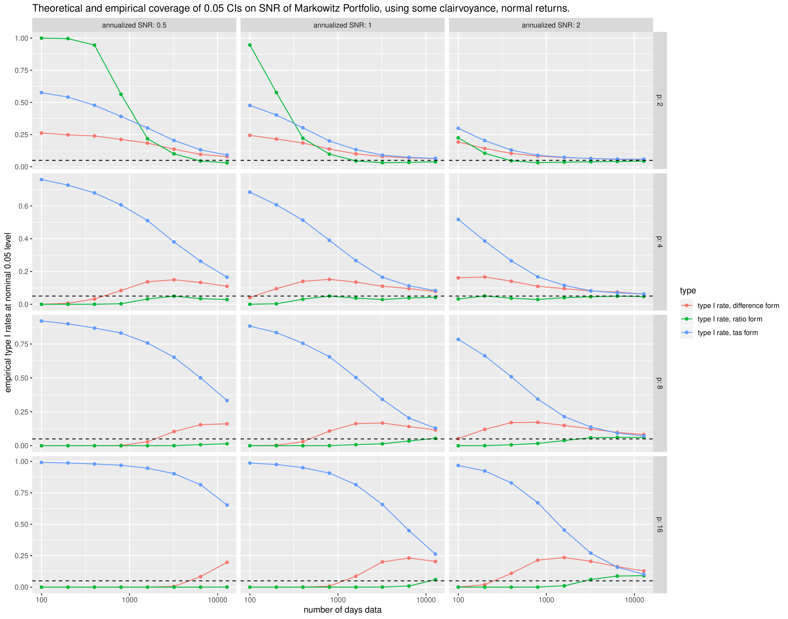
We test the confidence intervals of Theorem 3.11 and Equation 54 for random data. We draw returns from the multivariate normal distribution, for which $\kappa=1$ . We fix the number of days of data, $n$ , the number of assets, $p$ , and the optimal signal-noise ratio, ${\zeta}_{*}$ , and perform $2.5\times 10^{4}$ simulations. We then let $n$ vary from 100 to $1.28\times 10^{4}$ days; we let $p$ vary from 2 to 16; we let ${\zeta}_{*}$ vary from 0.5 to 2 in ‘annualized’ units (per square root year), where we assume 252 days per year. We compute the lower confidence limits on $\operatorname{SNR}\left(\boldsymbol{\nu};\mathsf{\Theta},0\right)$ , the signal-noise ratio of the sample Markowitz portfolio based on the difference and ratio forms from the theorem. The confidence limtis are computed very optimistically, by using the actual ${\zeta}_{*}$ in the expressions for the mean and variance of ${\operatorname{SNR}\left({{\mathsf{\hat{\Theta}}}^{-1}};\mathsf{\Theta},0\right)-{\hat{\zeta}}_{*}}$ and ${\operatorname{SNR}\left({{\mathsf{\hat{\Theta}}}^{-1}};\mathsf{\Theta},0\right)/{\hat{\zeta}}_{*}}$ . For the ‘TAS’ form of confidence limit, we use ${\hat{\zeta}}_{*}$ once in the non-centrality parameter, but otherwise use the actual ${\zeta}_{*}$ when computing parameters. Thus while this does not test the confidence limits in the way they would be practically used (e.g., Equation 59), the results are sufficiently discouraging even with this bit of clairvoyance to recommend against their general use.

We compute the lower 0.05 confidence limit based on the difference and ratio forms and the ‘TAS’ transform. We then compute the empirical type I rate. These are plotted against $n$ in Figure 1. We show facet columns for ${\zeta}_{*}$ , and facet rows for $p$ . The confidence intervals fail to achieve nominal coverage except perhaps for the largest values of $n$ , though these are much larger than would be used in practice.

Refer to caption — Figure 1: The empirical type I rate of three different one-sided confidence intervals for $\operatorname{SNR}\left({{\mathsf{\hat{\Theta}}}^{-1}};\mathsf{\Theta},0\right)$ , the signal-noise ratio of the Markowitz portfolio are shown, where the nominal type I rate is $0.05$ . The daily returns are drawn from multivariate normal distribution with varying ${\zeta}_{*}$ , $n$ , and $p$ . The confidence intervals generally fail to achieve the nominal rate except for unrealistically large values of $n$ .

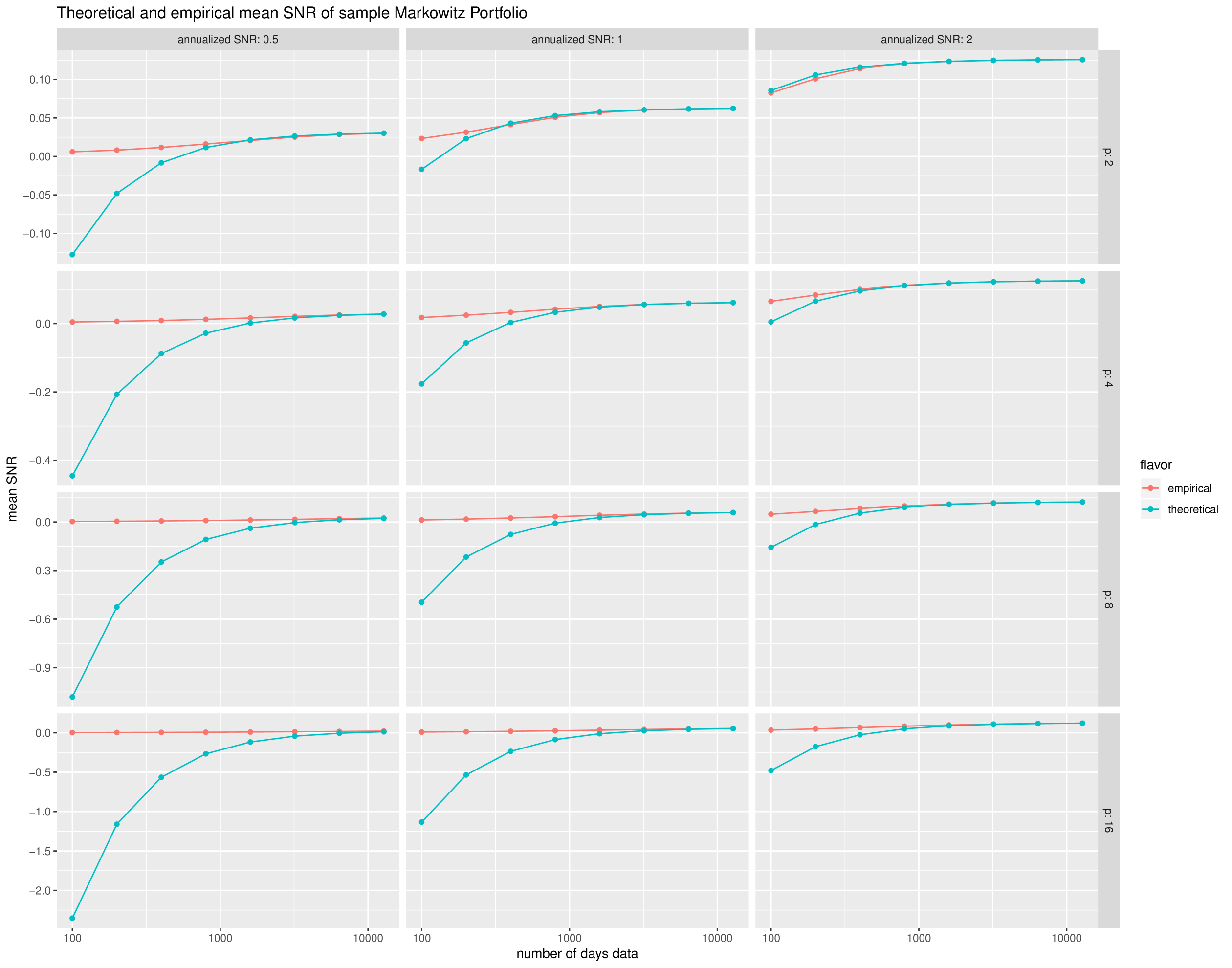
As a check, we also compare the empirical mean of the signal-noise ratio of the Markowitz portfolio from our experiments with the theoretical asymptotic value from Theorem 3.11, namely

\frac{\left(\kappa{\zeta}^{2}_{*}+1\right)\left(1-p\right)}{2n{\zeta}_{*}}.

We plot the empirical and theoretical means in Figure 2, again versus $n$ with facet columns for ${\zeta}_{*}$ , and facet rows for $p$ . The theoretical asymptotic value gives a good approximation for larger sample sizes, but ‘only’ around 6 years of daily data are required. Note that the theoretical value gets worse as $n{\zeta}_{*}\to 0$ , as one would expect: the signal-noise ratio of any portfolio must be no greater than ${\zeta}_{*}$ in absolute value, but the theoretical value goes to $-\infty$ .

7.1.2 Elliptical Returns

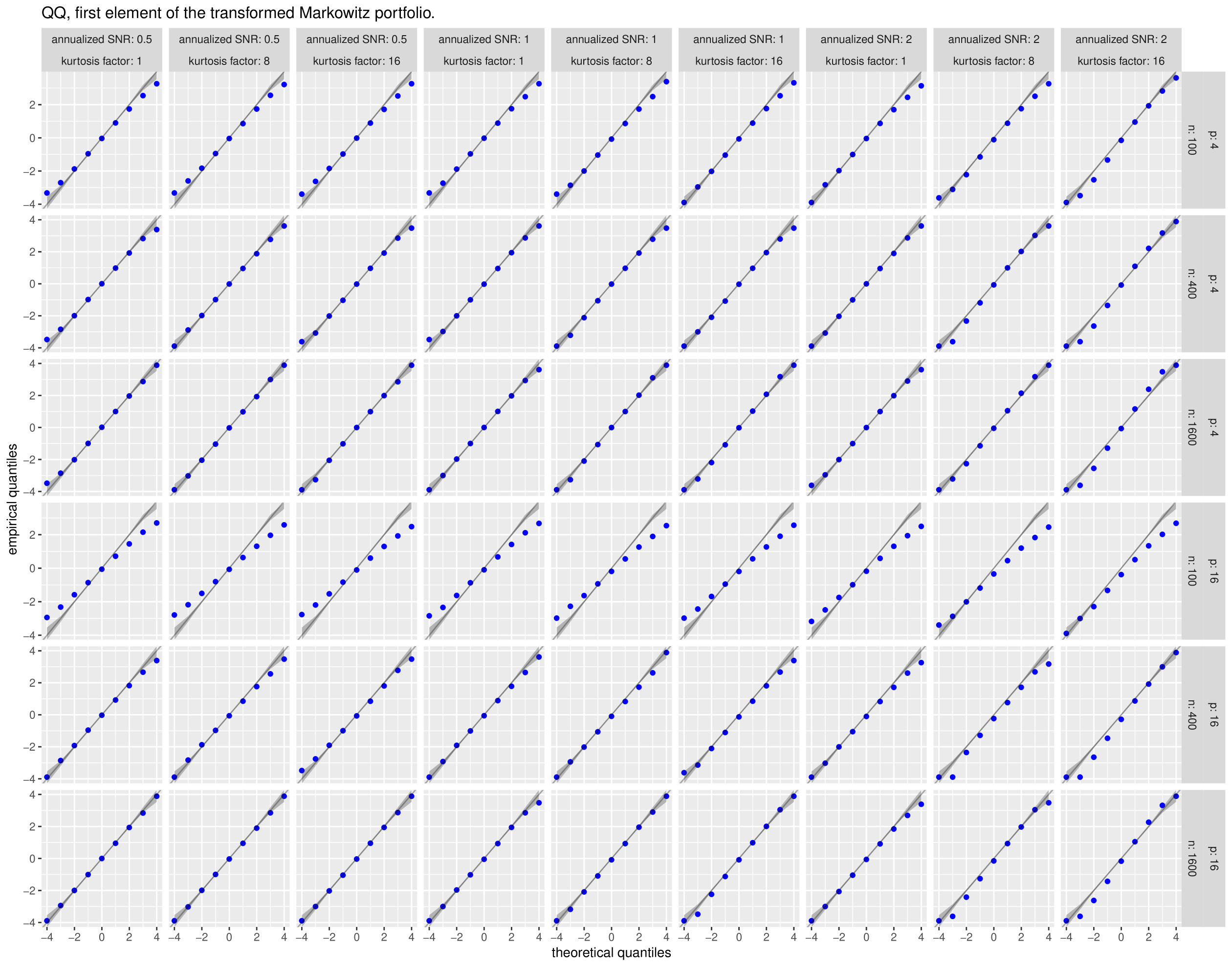
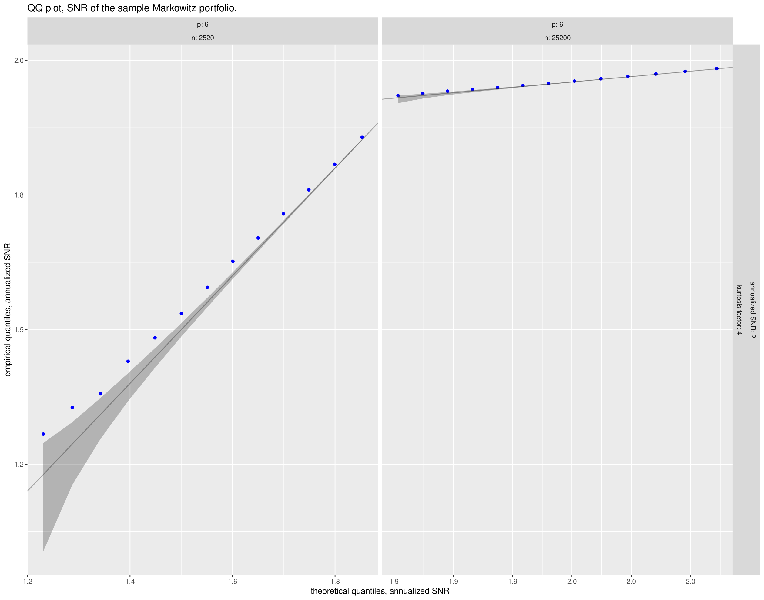
We now test Equation 50 via simulation. We fix the number of days of data, $n$ , the number of assets, $p$ , and the optimal signal-noise ratio, ${\zeta}_{*}$ , and the kurtosis factor, $\kappa$ , and perform $10^{4}$ simulations. We let $n$ vary from 100 to $1600$ days; we let $p$ vary from 4 to 16; we let $\kappa$ vary from 1 to 16; we let ${\zeta}_{*}$ vary from 0.5 to 2 in ‘annualized’ units (per square root year), where we assume 252 days per year. When $\kappa=1$ we draw from a multivariate normal distribution; when $\kappa>1$ , we draw from a multivariate shifted $t$ distribution.

For each simulation, we collect the first and last elements of the vector

\sqrt{n}\left({\mathsf{Q}{{\mathsf{\Sigma}}^{\top/2}}{\boldsymbol{\hat{\nu}}}_{{}*}}-{{\zeta}_{*}{\boldsymbol{e}}_{1}}\right)\mathsf{D}^{-1/2}.

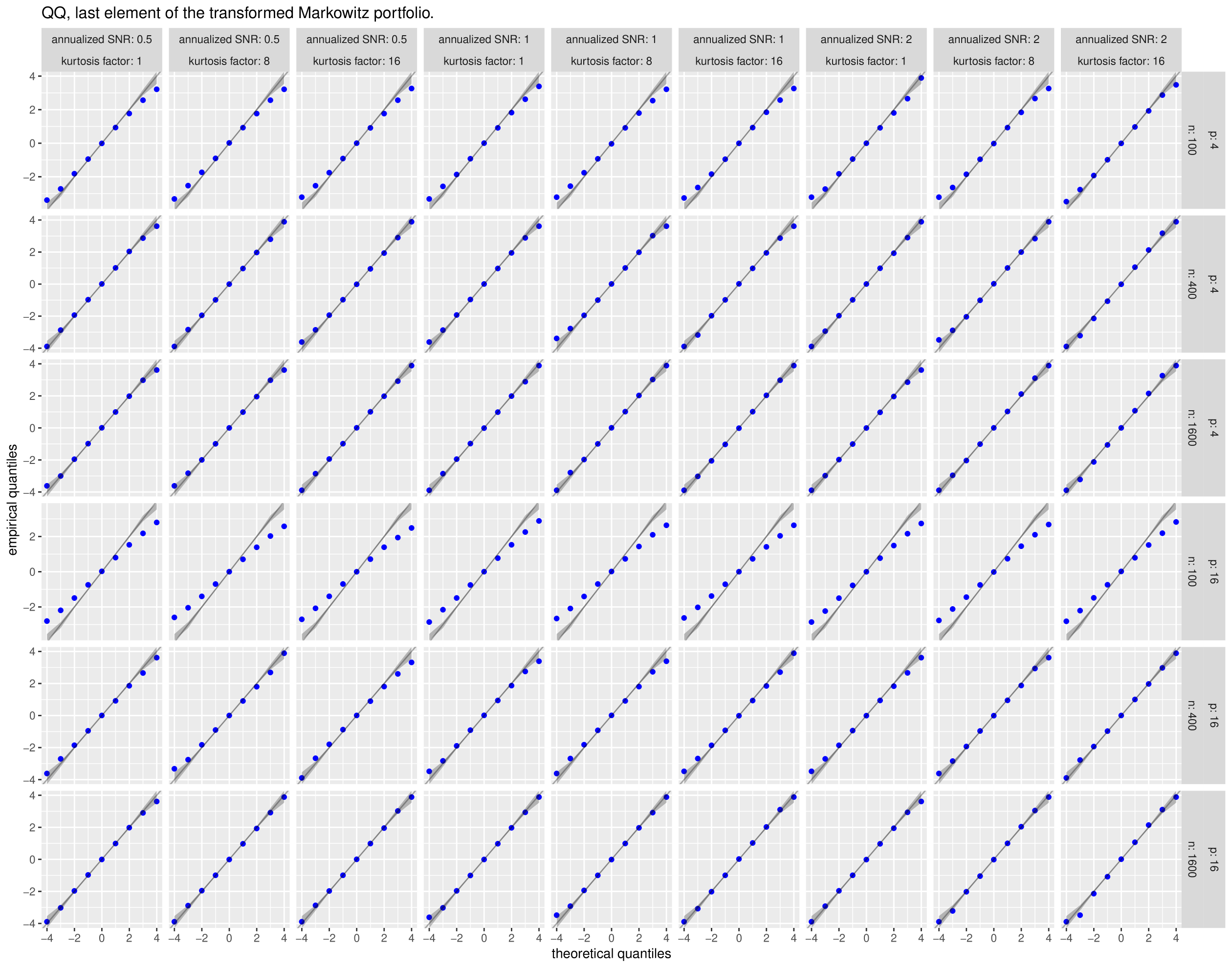
By Equation 50 these should be asymptotically distributed as a standard normal. In Figure 3 we give Q-Q plots of the first element of this vector versus quantiles of the standard normal for each setting of the simulation parameters. Rather than present the full Q-Q plot (each facet would contain 10,000 points), we take evenly spaced points between $-4$ and $4$ , then convert them into percentage points of the standard normal. We then find the empirical quantiles at those levels and plot the empirical quantiles against the selected theoretical. This allows us to also plot the pointwise confidence bands, which should be very small for the sample size, except at the periphery. Similarly, in Figure 4 we give the same kind of subsampled Q-Q plots of the last element of this vector.

With some exception, the Q-Q plots show a fair degree of support for normality when $n/p$ is reasonably large. For example, for $p=4$ , a sample of $n=400$ is apparently sufficient to get near normality for the last element of the vector. The first element of the vector, which one suspects is dependent on ${\zeta}_{*}$ , appears to suffer when ${\zeta}_{*}$ is larger.

We also check Equation 51 via a smaller set of simulations. We fix ${\zeta}_{*}=2$ in annualized units, $p=6$ , and $\kappa=4$ . We then test two different sample sizes: $n=2,520$ and $n=25,200$ , corresponding to 10 and 100 years of daily data, at a rate of $252$ days per year. For a given simulation we draw the appropriate number of days of independent returns from a shifted multivariate $t$ distribution. We compute the sample Markowitz portfolio and compute its signal-noise ratio, $\operatorname{SNR}\left({\boldsymbol{\hat{\nu}}}_{{}*}\right)$ . We perform this simulation 50,000 times for each setting of $n$ . We construct theoretical approximate quantiles of $\operatorname{SNR}\left({\boldsymbol{\hat{\nu}}}_{{}*}\right)$ using Equation 51, then plot the empirical quantiles versus the theoretical quantiles in Figure 5. It appears that more than 10 years of daily data (but fewer than 100 years worth) are required for this approximation to be any good. When the approximation breaks down, it tends to underestimate the true signal-noise ratio.

7.2 Fama French Three Factor Portfolios

The monthly returns of the Fama French 3 factor portfolios from Jul 1926 to Jul 2013 were downloaded from Quandl. [19, 41] The returns excess the risk-free rate (which is also given in the same data) are computed. The procedure of Britten-Jones is applied to get marginal $t$ statistics for each of the three assets. The marginal Wald statistics are also computed, first using the vanilla estimator of $\mathsf{\Omega}$ , then using a robust (HAC) estimator via the errors via the sandwich package. [68] These are presented in Table 2. The Wald statistics are slightly less optimistic than the Britten-Jones $t$ -statistics for the long MKT and short SMB positions. This is amplified when the HAC estimator is used.

Britten.Jones	4.10	0.30	-1.97
	MKT	HML	SMB
Wald	3.86	0.31	-1.92
Wald.HAC	3.51	0.27	-1.78

Table 2: The marginal

t

statistics of Britten-Jones [7] procedure, along with the Wald statistics from plugging in

\mathsf{\hat{\Theta}}

for

\mathsf{\Theta}

in Theorem 2.5, with ‘vanilla’ and HAC estimators of

\mathsf{\Omega}

, are shown for 1045 months of excess returns of the three Fama-French portfolios.

7.2.1 Incorporating conditional heteroskedasticity

A rolling estimate of general market volatility is computed by taking the 11 month FIR mean of the median absolute return of the three portfolios, delayed by one month. The model of ‘constant maximal Sharpe ratio’ (i.e., Equation 76) is assumed, where ${{s}_{i}}$ is the inverse of this estimated volatility. This is equivalent to dividing the returns by the estimated volatility, then applying the unconditional estimator.

The marginal Wald statistics are presented in Table 3, and are more ‘confident’ in the long MKT position, and short SMB position, with little evidence to support a long or short position in HML.

	MKT	HML	SMB
HAC.wald.wt	4.51	0.62	-2.93

Table 3: The marginal Wald statistics computed from plugging in

\mathsf{\hat{\Theta}}

for

\mathsf{\Theta}

in Theorem 2.5, with a HAC estimator of

\mathsf{\Omega}

, are shown for 1045 months of excess returns of the three Fama-French portfolios. To adjust for heteroskedasticity, returns are divided by a lagged volatility estimate based on 11 previous months of returns of the three portfolios.

7.2.2 Conditional expectation

The Shiller cyclically adjusted price/earnings data (CAPE) are downloaded from Quandl. [41] The CAPE data are delayed by a month so that they qualify as features which could be used in the investment decision. That is, we are testing a model where CAPE are used to predict returns, not ‘explain’ them, contemporaneously. The CAPE data are centered by subtracting the mean. The marginal Wald statistics, computed using a HAC estimator for $\mathsf{\Omega}$ , for the 6 elements of the Markowitz coefficient matrix are presented in Table 4, and indicate a significant unconditional long MKT position; when CAPE is above the long term average value of 17.54, decreasing the position in MKT is warranted.

	MKT	HML	SMB
Intercept	2.22	0.59	-1.33
CAPE	-2.46	-1.13	-0.70

Table 4: The marginal Wald statistics of the Markowitz coefficient computed from plugging in

\mathsf{\hat{\Theta}}

for

\mathsf{\Theta}

in Theorem 4.12, with a HAC estimator of

\mathsf{\Omega}

, are shown for 1045 months of excess returns of the three Fama-French portfolios. The Shiller CAPE data are delayed by a month, and centered. No adjustments for conditional heteroskedasticity are performed.

	MKT	HML	SMB
Intercept	3.49	0.27	-1.77
del.CAPE	1.19	0.03	2.52

Table 5: The marginal Wald statistics of the Markowitz coefficient computed from plugging in

\mathsf{\hat{\Theta}}

for

\mathsf{\Theta}

in Theorem 4.12, with a HAC estimator of

\mathsf{\Omega}

, are shown for 1045 months of excess returns of the three Fama-French portfolios. The Shiller CAPE data are delayed by a month, and the first difference is computed. No adjustments for conditional heteroskedasticity are performed.

The CAPE data change at a very low frequency. It is possible that the changes in the CAPE data are predictive of future returns. The Wald statistics of the Markowitz coefficient using the first difference in monthly CAPE dataa, delayed by a month, are presented in Table 5. These suggest a long unconditional position in MKT, with the differences in CAPE providing a ‘timing’ signal for an unconditional short SMB position.

7.2.3 Attribution of error

Theorem 2.5 gives the asymptotic distribution of ${{\mathsf{\hat{\Theta}}}^{-1}}$ , which contains the (negative) Markowitz portfolio and the precision matrix. This allows one to estimate the amount of error in the Markowitz portfolio which is attributable to mis-estimation of the covariance. The remainder one can attribute to mis-estimation of the mean vector, which, is typically implicated as the leading effect. [8]

The computation is performed as follows: the estimated covariance of $\operatorname{vech}\left({{\mathsf{\hat{\Theta}}}^{-1}}\right)$ is turned into a correlation matrix in the usual way³³3That is, by a Hadamard divide of the rank one matrix of the outer product of the diagonal. Or, more practically, by the R function cov2cor.. This gives a correlation matrix, call it $\mathsf{R}$ , some of the elements of which correspond to the negative Markowitz portfolio, and some to the precision matrix. For a single element of the Markowitz portfolio, let $\boldsymbol{r}$ be a sub-column of $\mathsf{R}$ consisting of the column corresponding to that element of the Markowitz portfolio and the rows of the precision matrix. And let $\mathsf{R}_{\mathsf{\Sigma}}$ be the sub-matrix of $\mathsf{R}$ corresponding to the precision matrix. The multiple correlation coefficient is then ${{\boldsymbol{r}}^{\top}}\mathsf{R}_{\mathsf{\Sigma}}^{-1}\boldsymbol{r}$ . This is an ‘R-squared’ number between zero and one, estimating the proportion of variance in that element of the Markowitz portfolio ‘explained’ by error in the precision matrix.

	vanilla	weighted
MKT	41 %	32 %
HML	11 %	6.8 %
SMB	29 %	13 %

Table 6: Estimated multiple correlation coefficients for the three elements of the Markowitz portfolio are presented. These are the percentage of error attributable to mis-estimation of the precision matrix. HAC estimators for

\mathsf{\Omega}

are used for both. In the ‘vanilla’ column, no adjustments are made for conditional heteroskedasticity, while in the ‘weighted’ column, returns are divided by the volatility estimate.

Here, for each of the members of the vanilla Markowitz portfolio on the 3 assets, this squared coefficient of multiple correlation, is expressed as percents in Table 6. A HAC estimator for $\mathsf{\Omega}$ is used. In the ‘weighted’ column, the returns are divided by the rolling estimate of volatility described above, assuming a model of ‘constant maximal Sharpe ratio’. We can claim, then, that approximately 41 percent of the error in the MKT position is due to mis-estimation of the precision matrix.

References

Anderson [2003] T. W. Anderson. An Introduction to Multivariate Statistical Analysis. Wiley Series in Probability and Statistics. Wiley, 2003. ISBN 9780471360919. URL http://books.google.com/books?id=Cmm9QgAACAAJ.
Andrews [2001] Donald WK Andrews. Testing when a parameter is on the boundary of the maintained hypothesis. Econometrica, 69(3):683–734, 2001. URL http://citeseerx.ist.psu.edu/viewdoc/download?doi=10.1.1.222.2587&rep=rep1&type=pdf.
Bodnar and Okhrin [2011] Taras Bodnar and Yarema Okhrin. On the product of inverse Wishart and normal distributions with applications to discriminant analysis and portfolio theory. Scandinavian Journal of Statistics, 38(2):311–331, 2011. ISSN 1467-9469. doi: 10.1111/j.1467-9469.2011.00729.x. URL http://dx.doi.org/10.1111/j.1467-9469.2011.00729.x.
Bollerslev [1987] Tim Bollerslev. A conditionally heteroskedastic time series model for speculative prices and rates of return. The Review of Economics and Statistics, 69(3):pp. 542–547, 1987. ISSN 00346535. URL http://www.jstor.org/stable/1925546.
Brandt [2009] Michael W Brandt. Portfolio choice problems. Handbook of financial econometrics, 1:269–336, 2009. URL https://faculty.fuqua.duke.edu/~mbrandt/papers/published/portreview.pdf.
Brandt and Santa-Clara [2006] Michael W. Brandt and Pedro Santa-Clara. Dynamic portfolio selection by augmenting the asset space. The Journal of Finance, 61(5):2187–2217, 2006. ISSN 1540-6261. doi: 10.1111/j.1540-6261.2006.01055.x. URL http://faculty.fuqua.duke.edu/~mbrandt/papers/published/condport.pdf.
Britten-Jones [1999] Mark Britten-Jones. The sampling error in estimates of mean-variance efficient portfolio weights. The Journal of Finance, 54(2):655–671, 1999. URL http://www.jstor.org/stable/2697722.
Chopra and Ziemba [1993] Vijay Kumar Chopra and William T. Ziemba. The effect of errors in means, variances, and covariances on optimal portfolio choice. The Journal of Portfolio Management, 19(2):6–11, 1993. URL http://faculty.fuqua.duke.edu/~charvey/Teaching/BA453_2006/Chopra_The_effect_of_1993.pdf.
Cochrane [2001] John Howland Cochrane. Asset pricing. Princeton Univ. Press, Princeton [u.a.], 2001. ISBN 0691074984. URL http://press.princeton.edu/titles/7836.html.
Connor [1997] Gregory Connor. Sensible return forecasting for portfolio management. Financial Analysts Journal, 53(5):pp. 44–51, 1997. ISSN 0015198X. URL https://faculty.fuqua.duke.edu/~charvey/Teaching/BA453_2006/Connor_Sensible_Return_Forecasting_1997.pdf.
Cont [2001] Rama Cont. Empirical properties of asset returns: stylized facts and statistical issues. Quantitative Finance, 1(2):223–236, 2001. doi: 10.1080/713665670. URL http://personal.fmipa.itb.ac.id/khreshna/files/2011/02/cont2001.pdf.
Cragg [1983] J. G. Cragg. More efficient estimation in the presence of heteroscedasticity of unknown form. Econometrica, 51(3):pp. 751–763, 1983. ISSN 00129682. URL http://www.jstor.org/stable/1912156.
DeMiguel et al. [2009] Victor DeMiguel, Lorenzo Garlappi, and Raman Uppal. Optimal versus naive diversification: How inefficient is the 1/N portfolio strategy? Review of Financial Studies, 22(5):1915–1953, 2009. URL http://faculty.london.edu/avmiguel/DeMiguel-Garlappi-Uppal-RFS.pdf.
DeMiguel et al. [2013] Victor DeMiguel, Alberto Martin-Utrera, and Francisco J Nogales. Size matters: Optimal calibration of shrinkage estimators for portfolio selection. Journal of Banking & Finance, 2013. URL http://faculty.london.edu/avmiguel/DMN-2011-07-21.pdf.
Dempster [1972] A. P. Dempster. Covariance selection. Biometrics, 28(1):pp. 157–175, 1972. ISSN 0006341X. URL http://www.jstor.org/stable/2528966.
Duncan [1983] Gregory M. Duncan. Estimation and inference for heteroscedastic systems of equations. International Economic Review, 24(3):pp. 559–566, 1983. ISSN 00206598. URL http://www.jstor.org/stable/2648786.
Fabozzi et al. [2007] F. J. Fabozzi, P. N. Kolm, D. Pachamanova, and S. M. Focardi. Robust Portfolio Optimization and Management. Frank J. Fabozzi series. Wiley, 2007. ISBN 9780470164891. URL http://books.google.com/books?id=PUnRxEBIFb4C.
Fackler [2005] Paul L. Fackler. Notes on matrix calculus. Privately Published, 2005. URL http://www4.ncsu.edu/~pfackler/MatCalc.pdf.
Fama and French [1992] Eugene F. Fama and Kenneth R. French. The cross-section of expected stock returns. Journal of Finance, 47(2):427, 1992. URL http://www.jstor.org/stable/2329112.
Giri [1964] Narayan C. Giri. On the likelihood ratio test of a normal multivariate testing problem. The Annals of Mathematical Statistics, 35(1):181–189, 1964. doi: 10.1214/aoms/1177703740. URL http://projecteuclid.org/euclid.aoms/1177703740.
Hall [1983] Peter Hall. Chi squared approximations to the distribution of a sum of independent random variables. The Annals of Probability, 11(4):pp. 1028–1036, 1983. ISSN 00911798. URL http://www.jstor.org/stable/2243514.
Herold and Maurer [2004] Ulf Herold and Raimond Maurer. Tactical asset allocation and estimation risk. Financial Markets and Portfolio Management, 18(1):39–57, 2004. ISSN 1555-4961. doi: 10.1007/s11408-004-0104-2. URL http://dx.doi.org/10.1007/s11408-004-0104-2.
Huberman and Kandel [1987] Gur Huberman and Shmuel Kandel. Mean-variance spanning. The Journal of Finance, 42(4):pp. 873–888, 1987. ISSN 00221082. URL http://www.jstor.org/stable/2328296.
Iwashita [1997] Toshiya Iwashita. Asymptotic null and nonnull distribution of Hotelling’s $T^{2}$ -statistic under the elliptical distribution. Journal of Statistical Planning and Inference, 61(1):85 – 104, 1997. ISSN 0378-3758. doi: https://doi.org/10.1016/S0378-3758(96)00153-X. URL http://www.sciencedirect.com/science/article/pii/S037837589600153X.
Iwashita and Siotani [1994] Toshiya Iwashita and Minoru Siotani. Asymptotic distributions of functions of a sample covariance matrix under the elliptical distribution. Canadian Journal of Statistics, 22(2):273–283, 1994. ISSN 1708-945X. doi: 10.2307/3315589. URL http://dx.doi.org/10.2307/3315589.
Izenman [1975] Alan Julian Izenman. Reduced-rank regression for the multivariate linear model. Journal of Multivariate Analysis, 5(2):248 – 264, 1975. ISSN 0047-259X. doi: http://dx.doi.org/10.1016/0047-259X(75)90042-1. URL http://www.sciencedirect.com/science/article/pii/0047259X75900421.
Jobson and Korkie [1981] J. D. Jobson and Bob M. Korkie. Performance hypothesis testing with the Sharpe and Treynor measures. The Journal of Finance, 36(4):pp. 889–908, 1981. ISSN 00221082. URL http://www.jstor.org/stable/2327554.
Johnstone [2009] Iain M. Johnstone. Approximate null distribution of the largest root in multivariate analysis. Annals of Applied Statistics, 3(4):1616–1633, 2009. URL http://projecteuclid.org/euclid.aoas/1267453956.
Kan [2008] Raymond Kan. From moments of sum to moments of product. Journal of Multivariate Analysis, 99(3):542 – 554, 2008. ISSN 0047-259X. doi: https://doi.org/10.1016/j.jmva.2007.01.013. URL http://www.sciencedirect.com/science/article/pii/S0047259X07000139.
Kan and Zhou [2012] Raymond Kan and GuoFu Zhou. Tests of mean-variance spanning. Annals of Economics and Finance, 13(1), 2012. URL http://www.aeconf.net/Articles/May2012/aef130105.pdf.
Kinkawa [2010] Takuya Kinkawa. Estimation of optimal portfolio weights using shrinkage technique. 2010. URL http://papers.ssrn.com/sol3/papers.cfm?abstract_id=1576052.
Ledoit and Wolf [2008] Olivier Ledoit and Michael Wolf. Robust performance hypothesis testing with the Sharpe ratio. Journal of Empirical Finance, 15(5):850–859, Dec 2008. ISSN 0927-5398. doi: http://dx.doi.org/10.1016/j.jempfin.2008.03.002. URL http://www.ledoit.net/jef2008_abstract.htm.
Leung and Wong [2008] Pui-Lam Leung and Wing-Keung Wong. On testing the equality of multiple Sharpe ratios, with application on the evaluation of iShares. Journal of Risk, 10(3):15–30, 2008. URL http://www.risk.net/digital_assets/4760/v10n3a2.pdf.
Lo [2002] Andrew W. Lo. The statistics of Sharpe ratios. Financial Analysts Journal, 58(4), July/August 2002. URL http://ssrn.com/paper=377260.
Magnus and Neudecker [1979] Jan R. Magnus and H. Neudecker. The commutation matrix: Some properties and applications. Ann. Statist., 7(2):381–394, 03 1979. doi: 10.1214/aos/1176344621. URL https://doi.org/10.1214/aos/1176344621.
Magnus and Neudecker [1980] Jan R. Magnus and H. Neudecker. The elimination matrix: Some lemmas and applications. SIAM Journal on Algebraic Discrete Methods, 1(4):422–449, dec 1980. doi: 10.1137/0601049. URL http://www.janmagnus.nl/papers/JRM008.pdf.
Magnus and Neudecker [2007] Jan R. Magnus and H. Neudecker. Matrix Differential Calculus with Applications in Statistics and Econometrics. Wiley Series in Probability and Statistics: Texts and References Section. Wiley, 3rd edition, 2007. ISBN 9780471986331. URL http://www.janmagnus.nl/misc/mdc2007-3rdedition.
Markowitz [1952] Harry Markowitz. Portfolio selection. The Journal of Finance, 7(1):pp. 77–91, 1952. ISSN 00221082. URL http://www.jstor.org/stable/2975974.
Markowitz [1999] Harry Markowitz. The early history of portfolio theory: 1600-1960. Financial Analysts Journal, pages 5–16, 1999. URL http://www.jstor.org/stable/10.2307/4480178.
Markowitz [2012] Harry Markowitz. Foundations of portfolio theory. The Journal of Finance, 46(2):469–477, 2012. URL http://onlinelibrary.wiley.com/doi/10.1111/j.1540-6261.1991.tb02669.x/abstract.
McTaggart and Daroczi [2014] Raymond McTaggart and Gergely Daroczi. Quandl: Quandl Data Connection, 2014. URL http://CRAN.R-project.org/package=Quandl. R package version 2.4.0.
Mertens [2002] Elmar Mertens. Comments on variance of the IID estimator in Lo (2002). Technical report, Working Paper University of Basel, Wirtschaftswissenschaftliches Zentrum, Department of Finance, 2002. URL http://www.elmarmertens.com/research/discussion/soprano01.pdf.
Merton [1980] Robert C. Merton. On estimating the expected return on the market: An exploratory investigation. Working Paper 444, National Bureau of Economic Research, February 1980. URL http://www.nber.org/papers/w0444.
Michaud [1989] Richard O. Michaud. The Markowitz optimization enigma: is ‘optimized’ optimal? Financial Analysts Journal, pages 31–42, 1989. URL http://newfrontieradvisors.com/Research/Articles/documents/markowitz-optimization-enigma-010189.pdf.
Muller and Peterson [1984] Keith E. Muller and Bercedis L. Peterson. Practical methods for computing power in testing the multivariate general linear hypothesis. Computational Statistics & Data Analysis, 2(2):143–158, 1984. ISSN 0167-9473. doi: 10.1016/0167-9473(84)90002-1. URL http://www.sciencedirect.com/science/article/pii/0167947384900021.
Mulvey et al. [2003] John M Mulvey, William R Pauling, and Ronald E Madey. Advantages of multiperiod portfolio models. The Journal of Portfolio Management, 29(2):35–45, 2003. doi: 10.3905/jpm.2003.319871. URL http://dx.doi.org/10.3905/jpm.2003.319871#sthash.oKQ9cHFy.jsYuZ7C2.dpuf.
Nelson [1991] Daniel B. Nelson. Conditional heteroskedasticity in asset returns: A new approach. Econometrica, 59(2):pp. 347–370, 1991. ISSN 00129682. URL http://finance.martinsewell.com/stylized-facts/distribution/Nelson1991.pdf.
Nocedal and Wright [2006] J. Nocedal and S. J. Wright. Numerical Optimization. Springer series in operations research and financial engineering. Springer, 2006. ISBN 9780387400655. URL http://books.google.com/books?id=VbHYoSyelFcC.
O’Brien and Shieh [1999] Ralph G. O’Brien and Gwowen Shieh. Pragmatic, unifying algorithm gives power probabilities for common F tests of the multivariate general linear hypothesis, 1999. URL http://www.bio.ri.ccf.org/Power/.
Okhrin and Schmid [2006] Yarema Okhrin and Wolfgang Schmid. Distributional properties of portfolio weights. Journal of Econometrics, 134(1):235–256, 2006. URL http://www.sciencedirect.com/science/article/pii/S0304407605001442.
Paulsen and Söhl [2016] Dirk Paulsen and Jakob Söhl. Noise fit, estimation error and a Sharpe information criterion, 2016. URL http://arxiv.org/abs/1602.06186.
Pav [2014] Steven E. Pav. Bounds on portfolio quality. Privately Published, 2014. URL http://arxiv.org/abs/1409.5936.
Pav [2017] Steven E. Pav. A short Sharpe course. Privately Published, 2017. URL https://papers.ssrn.com/sol3/papers.cfm?abstract_id=3036276.
Petersen and Pedersen [2012] Kaare Brandt Petersen and Michael Syskind Pedersen. The matrix cookbook, nov 2012. URL http://www2.imm.dtu.dk/pubdb/p.php?3274. Version 20121115.
Press [2012] S. J. Press. Applied Multivariate Analysis: Using Bayesian and Frequentist Methods of Inference. Dover Publications, Incorporated, 2012. ISBN 9780486139388. URL http://books.google.com/books?id=WneJJEHYHLYC.
Rall [1981] L. B. Rall. Automatic Differentiation: Techniques and Applications. Lecture Notes in Computer Science. Springer, 1981. ISBN 9783540108610. URL http://books.google.com/books?id=5QxRAAAAMAAJ.
Rao [1952] C. Radhakrishna Rao. Advanced Statistical Methods in Biometric Research. John Wiley and Sons, 1952. URL http://books.google.com/books?id=HvFLAAAAMAAJ.
Rencher [2002] Alvin C. Rencher. Methods of Multivariate Analysis. Wiley series in probability and mathematical statistics. Probability and mathematical statistics. J. Wiley, 2002. ISBN 9780471418894. URL http://books.google.com/books?id=SpvBd7IUCxkC.
Shieh [2003] Gwowen Shieh. A comparative study of power and sample size calculations for multivariate general linear models. Multivariate Behavioral Research, 38(3):285–307, 2003. doi: 10.1207/S15327906MBR3803˙01. URL http://www.tandfonline.com/doi/abs/10.1207/S15327906MBR3803_01.
Shieh [2005] Gwowen Shieh. Power and sample size calculations for multivariate linear models with random explanatory variables. Psychometrika, 70(2):347–358, 2005. doi: 10.1007/s11336-003-1094-0. URL https://ir.nctu.edu.tw/bitstream/11536/13599/1/000235235100007.pdf.
Silvapulle and Sen [2005] Mervyn J. Silvapulle and Pranab Kumar Sen. Constrained statistical inference : inequality, order, and shape restrictions. Wiley-Interscience, Hoboken, N.J., 2005. ISBN 0471208272. URL http://books.google.com/books?isbn=0471208272.
Tang [1994] Dei-In Tang. Uniformly more powerful tests in a one-sided multivariate problem. Journal of the American Statistical Association, 89(427):pp. 1006–1011, 1994. ISSN 01621459. URL http://www.jstor.org/stable/2290927.
Timm [2002] N. H. Timm. Applied multivariate analysis: methods and case studies. Springer Texts in Statistics. Physica-Verlag, 2002. ISBN 9780387227719. URL http://amzn.to/TMdgaE.
Vignat and Bhatnagar [2007] C. Vignat and S. Bhatnagar. An extension of Wick’s theorem, 2007. URL http://arxiv.org/abs/0709.1999.
Wasserman [2004] Larry Wasserman. All of Statistics: A Concise Course in Statistical Inference. Springer Texts in Statistics. Springer, 2004. ISBN 9780387402727. URL http://books.google.com/books?id=th3fbFI1DaMC.
Wilks [1938] S. S. Wilks. The large-sample distribution of the likelihood ratio for testing composite hypotheses. The Annals of Mathematical Statistics, 9(1):pp. 60–62, 1938. ISSN 00034851. URL http://www.jstor.org/stable/2957648.
Yanagihara [2001] Hirokazu Yanagihara. Asymptotic expansions of the null distributions of three test statistics in a nonnormal GMANOVA model. Hiroshima Mathematical Journal, 31(2):213–262, 07 2001. URL http://projecteuclid.org/euclid.hmj/1151105700.
Zeileis [2004] Achim Zeileis. Econometric computing with HC and HAC covariance matrix estimators. Journal of Statistical Software, 11(10):1–17, 11 2004. ISSN 1548-7660. URL http://www.jstatsoft.org/v11/i10.

Appendix A Matrix Derivatives

Lemma A.1 (Derivatives).

Given conformable, symmetric, matrices $\mathsf{X}$ , $\mathsf{Y}$ , $\mathsf{Z}$ , and constant matrix $\mathsf{J}$ , define

{f}_{\mathcal{P}}\left(\mathsf{X};\mathsf{J}\right)=_{\operatorname{df}}-\left({{{\left({{\mathsf{J}}^{\top}}\mathsf{X}\mathsf{J}\right)}^{-1}}}\otimes{{{\left({{\mathsf{J}}^{\top}}\mathsf{X}\mathsf{J}\right)}^{-1}}}\right)\left({{{\mathsf{J}}^{\top}}}\otimes{{{\mathsf{J}}^{\top}}}\right).

Then

$\displaystyle\frac{\mathrm{d}{{{\left({{\mathsf{J}}^{\top}}\mathsf{X}\mathsf{J}\right)}^{-1}}}}{\mathrm{d}\mathsf{Z}}$	$\displaystyle={f}_{\mathcal{P}}\left(\mathsf{X};\mathsf{J}\right)\frac{\mathrm{d}{\mathsf{X}}}{\mathrm{d}\mathsf{Z}}.$	(121)
$\displaystyle\frac{\mathrm{d}{\mathsf{X}\mathsf{Y}}}{\mathrm{d}\mathsf{Z}}$	$\displaystyle=\left(\mathsf{I}\otimes\mathsf{X}\right)\frac{\mathrm{d}{\mathsf{Y}}}{\mathrm{d}\mathsf{Z}}+\left({{\mathsf{Y}}^{\top}}\otimes\mathsf{I}\right)\frac{\mathrm{d}{\mathsf{X}}}{\mathrm{d}\mathsf{Z}}.$	(122)
$\displaystyle\frac{\mathrm{d}{\mathsf{X}{{\mathsf{X}}^{\top}}}}{\mathrm{d}\mathsf{Z}}$	$\displaystyle=\left(\mathsf{I}+\mathsf{K}\right)\left(\mathsf{X}\otimes\mathsf{I}\right)\frac{\mathrm{d}{\mathsf{X}}}{\mathrm{d}\mathsf{Z}}.$	(123)
$\displaystyle\frac{\mathrm{d}{\operatorname{tr}\left(\mathsf{X}\mathsf{Y}\right)}}{\mathrm{d}\mathsf{Z}}$	$\displaystyle={{\operatorname{vec}\left({{\mathsf{X}}^{\top}}\right)}^{\top}}\frac{\mathrm{d}{\mathsf{Y}}}{\mathrm{d}\mathsf{Z}}+{{\operatorname{vec}\left(\mathsf{Y}\right)}^{\top}}\frac{\mathrm{d}{{{\mathsf{X}}^{\top}}}}{\mathrm{d}\mathsf{Z}}.$	(124)
$\displaystyle\frac{\mathrm{d}{\left\|\mathsf{X}\right\|}}{\mathrm{d}\mathsf{Z}}$	$\displaystyle=\left\|\mathsf{X}\right\|{{\operatorname{vec}\left({{\mathsf{X}}^{-\top}}\right)}^{\top}}\frac{\mathrm{d}{\mathsf{X}}}{\mathrm{d}\mathsf{Z}}.$	(125)
$\displaystyle\frac{\mathrm{d}{\left\|\mathsf{X}\mathsf{Y}\right\|}}{\mathrm{d}\mathsf{Z}}$	$\displaystyle=\left\|\mathsf{X}\mathsf{Y}\right\|\left({{\operatorname{vec}\left({{\mathsf{X}}^{-\top}}\right)}^{\top}}\frac{\mathrm{d}{\mathsf{X}}}{\mathrm{d}\mathsf{Z}}+{{\operatorname{vec}\left({{\mathsf{Y}}^{-\top}}\right)}^{\top}}\frac{\mathrm{d}{\mathsf{Y}}}{\mathrm{d}\mathsf{Z}}\right).$	(126)
$\displaystyle\frac{\mathrm{d}{\left\|{{\left(\mathsf{X}\mathsf{Y}\right)}^{-1}}\right\|}}{\mathrm{d}\mathsf{Z}}$	$\displaystyle=\left\|\mathsf{X}\mathsf{Y}\right\|^{-1}\left({{\operatorname{vec}\left({{\mathsf{X}}^{-\top}}\right)}^{\top}}\frac{\mathrm{d}{\mathsf{X}}}{\mathrm{d}\mathsf{Z}}+{{\operatorname{vec}\left({{\mathsf{Y}}^{-\top}}\right)}^{\top}}\frac{\mathrm{d}{\mathsf{Y}}}{\mathrm{d}\mathsf{Z}}\right).$	(127)

Here $\mathsf{K}$ is the ’commutation matrix.’

Let ${\lambda}_{j}$ be the $j^{\text{th}}$ eigenvalue of $\mathsf{X}$ , with corresponding eigenvector ${\boldsymbol{\nu}}_{j}$ , normalized so that ${{{\boldsymbol{\nu}}_{j}}^{\top}}{\boldsymbol{\nu}}_{j}=1$ . Then

\displaystyle\frac{\mathrm{d}{{\lambda}_{j}}}{\mathrm{d}\mathsf{Z}}

\displaystyle=\left({{{{\boldsymbol{\nu}}_{j}}^{\top}}}\otimes{{{{\boldsymbol{\nu}}_{j}}^{\top}}}\right)\frac{\mathrm{d}{\mathsf{X}}}{\mathrm{d}\mathsf{Z}}.

(128)

Proof.

For Equation 121, write

\frac{\mathrm{d}{{{\left({{\mathsf{J}}^{\top}}\mathsf{X}\mathsf{J}\right)}^{-1}}}}{\mathrm{d}\mathsf{Z}}=\frac{\mathrm{d}{{{\left({{\mathsf{J}}^{\top}}\mathsf{X}\mathsf{J}\right)}^{-1}}}}{\mathrm{d}\left({{\mathsf{J}}^{\top}}\mathsf{X}\mathsf{J}\right)}\frac{\mathrm{d}{\left({{\mathsf{J}}^{\top}}\mathsf{X}\mathsf{J}\right)}}{\mathrm{d}\mathsf{Z}}.

Lemma 2.4 gives the derivative on the left; to get the derivative on the right, note that $\operatorname{vec}\left({{\mathsf{J}}^{\top}}\mathsf{X}\mathsf{J}\right)=\left({{{\mathsf{J}}^{\top}}}\otimes{{{\mathsf{J}}^{\top}}}\right)\operatorname{vec}\left(\mathsf{X}\right)$ , then use linearity of the derivative.

For Equation 122, write $\operatorname{vec}\left(\mathsf{X}\mathsf{Y}\right)=\left({{\mathsf{Y}}^{\top}}\otimes\mathsf{X}\right)\operatorname{vec}\left(\mathsf{I}\right)$ . Then consider the derivative of $\operatorname{vec}\left(\mathsf{X}\mathsf{Y}\right)$ with respect to any scalar $z$ :

\frac{\mathrm{d}{\operatorname{vec}\left(\mathsf{X}\mathsf{Y}\right)}}{\mathrm{d}z}=\frac{\mathrm{d}{\left({{\mathsf{Y}}^{\top}}\otimes\mathsf{X}\right)\operatorname{vec}\left(\mathsf{I}\right)}}{\mathrm{d}z}={{\operatorname{vec}}}^{-1}\left(\frac{\mathrm{d}{\left({{\mathsf{Y}}^{\top}}\otimes\mathsf{X}\right)}}{\mathrm{d}z}\right)\operatorname{vec}\left(\mathsf{I}\right),

where ${{\operatorname{vec}}}^{-1}\left(\cdot\right)$ is the inverse of $\operatorname{vec}\left(\cdot\right)$ . That is, ${{\operatorname{vec}}}^{-1}\left(\operatorname{vec}\left(\cdot\right)\right)$ is the identity over square matrices. (This wrinkle is needed because we have defined derivatives of matrices to be the derivative of their vectorization.)

For Equation 123, by Equation 122,

\begin{split}\frac{\mathrm{d}{\operatorname{vec}\left(\mathsf{X}{{\mathsf{X}}^{\top}}\right)}}{\mathrm{d}\operatorname{vec}\left(\mathsf{Z}\right)}&=\left(\mathsf{I}\otimes\mathsf{X}\right)\frac{\mathrm{d}{\operatorname{vec}\left({{\mathsf{X}}^{\top}}\right)}}{\mathrm{d}\operatorname{vec}\left(\mathsf{Z}\right)}+\left({\mathsf{X}}\otimes\mathsf{I}\right)\frac{\mathrm{d}{\operatorname{vec}\left(\mathsf{X}\right)}}{\mathrm{d}\operatorname{vec}\left(\mathsf{Z}\right)},\\ &=\left(\mathsf{I}\otimes\mathsf{X}\right)\mathsf{K}\frac{\mathrm{d}{\operatorname{vec}\left(\mathsf{X}\right)}}{\mathrm{d}\operatorname{vec}\left(\mathsf{Z}\right)}+\left({\mathsf{X}}\otimes\mathsf{I}\right)\frac{\mathrm{d}{\operatorname{vec}\left(\mathsf{X}\right)}}{\mathrm{d}\operatorname{vec}\left(\mathsf{Z}\right)}.\\ \end{split}

Now let $\mathsf{A}$ be any conformable square matrix. We have:

\left(\mathsf{I}\otimes\mathsf{X}\right)\mathsf{K}\operatorname{vec}\left(\mathsf{A}\right)=\left(\mathsf{I}\otimes\mathsf{X}\right)\operatorname{vec}\left({{\mathsf{A}}^{\top}}\right)=\operatorname{vec}\left(\mathsf{X}{{\mathsf{A}}^{\top}}\right)=\\ \mathsf{K}\operatorname{vec}\left(\mathsf{A}{{\mathsf{X}}^{\top}}\right)=\mathsf{K}\left(\mathsf{X}\otimes\mathsf{I}\right)\operatorname{vec}\left(\mathsf{A}\right).

Because $\mathsf{A}$ was arbitrary, we have $\left(\mathsf{I}\otimes\mathsf{X}\right)\mathsf{K}=\mathsf{K}\left(\mathsf{X}\otimes\mathsf{I}\right),$ and the result follows.

Using the product rule for Kronecker products [54], then using the vector identity again we have

\begin{split}\frac{\mathrm{d}{\operatorname{vec}\left(\mathsf{X}\mathsf{Y}\right)}}{\mathrm{d}z}&=\left({{\operatorname{vec}}}^{-1}\left(\frac{\mathrm{d}{{{\mathsf{Y}}^{\top}}}}{\mathrm{d}z}\right)\otimes\mathsf{X}+{{\mathsf{Y}}^{\top}}\otimes{{\operatorname{vec}}}^{-1}\left(\frac{\mathrm{d}{\mathsf{X}}}{\mathrm{d}z}\right)\right)\operatorname{vec}\left(\mathsf{I}\right),\\ &=\left(\mathsf{I}\otimes\mathsf{X}\right)\frac{\mathrm{d}{{\mathsf{Y}}}}{\mathrm{d}z}+\left({{\mathsf{Y}}^{\top}}\otimes\mathsf{I}\right)\frac{\mathrm{d}{\mathsf{X}}}{\mathrm{d}z}.\end{split}

Then apply this result to every element of $\operatorname{vec}\left(\mathsf{Z}\right)$ to get the result.

For Equation 124, write

\operatorname{tr}\left(\mathsf{X}\mathsf{Y}\right)={{\operatorname{vec}\left({{\mathsf{X}}^{\top}}\right)}^{\top}}\operatorname{vec}\left(\mathsf{Y}\right),

then use the product rule.

For Equation 125, first consider the derivative of $\left|\mathsf{X}\right|$ with respect to a scalar $z$ . This is known to take form: [54]

\frac{\mathrm{d}{\left|\mathsf{X}\right|}}{\mathrm{d}z}=\left|X\right|\operatorname{tr}\left({{\mathsf{X}}^{-1}}{{\operatorname{vec}}}^{-1}\left(\frac{\mathrm{d}{\mathsf{X}}}{\mathrm{d}z}\right)\right),

where the ${{\operatorname{vec}}}^{-1}\left(\cdot\right)$ is here because of how we have defined derivatives of matrices. Rewrite the trace as the dot product of two vectors:

\frac{\mathrm{d}{\left|\mathsf{X}\right|}}{\mathrm{d}z}=\left|X\right|{{\operatorname{vec}\left({{\mathsf{X}}^{-\top}}\right)}^{\top}}\frac{\mathrm{d}{\mathsf{X}}}{\mathrm{d}z}.

Using this to compute the derivative with respect to each element of $\operatorname{vec}\left(\mathsf{Z}\right)$ gives the result. Equation 126 follows from the scalar product rule since $\left|\mathsf{X}\mathsf{Y}\right|=\left|\mathsf{X}\right|\left|\mathsf{Y}\right|$ . Equation 127 then follows, using the scalar chain rule.

For Equation 128, the derivative of the $j^{\text{th}}$ eigenvalue of matrix $\mathsf{X}$ with respect to a scalar $z$ is known to be: [54, equation (67)]

\frac{\mathrm{d}{{\lambda}_{j}}}{\mathrm{d}z}={{{\boldsymbol{\nu}}_{j}}^{\top}}{{\operatorname{vec}}}^{-1}\left(\frac{\mathrm{d}{\mathsf{X}}}{\mathrm{d}z}\right){\boldsymbol{\nu}}_{j}.

Take the vectorization of this scalar, and rewrite it in Kronecker form:

\frac{\mathrm{d}{{\lambda}_{j}}}{\mathrm{d}z}=\left({{{{\boldsymbol{\nu}}_{j}}^{\top}}}\otimes{{{{\boldsymbol{\nu}}_{j}}^{\top}}}\right)\frac{\mathrm{d}{\mathsf{X}}}{\mathrm{d}z}.

Use this to compute the derivative of ${\lambda}_{j}$ with respect to each element of $\operatorname{vec}\left(\mathsf{Z}\right)$ .

∎

Lemma A.2 (Cholesky Derivatives).

Let $\mathsf{X}$ be a symmetric positive definite matrix. Let $\mathsf{Y}$ be its lower triangular Cholesky factor. That is, $\mathsf{Y}$ is the lower triangular matrix such that $\mathsf{Y}{{\mathsf{Y}}^{\top}}=\mathsf{X}$ . Then

\displaystyle\frac{\mathrm{d}{\operatorname{vech}\left(\mathsf{Y}\right)}}{\mathrm{d}\operatorname{vech}\left(\mathsf{X}\right)}

\displaystyle={{\left(\mathsf{L}\left(\mathsf{I}+\mathsf{K}\right)\left(\mathsf{Y}\otimes\mathsf{I}\right){{\mathsf{L}}^{\top}}\right)}^{-1}},

(129)

where $\mathsf{K}$ is the ’commutation matrix’. [37]

Proof.

By Equation 123 of Lemma A.1,

\frac{\mathrm{d}{\operatorname{vec}\left(\mathsf{Y}{{\mathsf{Y}}^{\top}}\right)}}{\mathrm{d}\operatorname{vec}\left(\mathsf{Y}\right)}=\left(\mathsf{I}+\mathsf{K}\right)\left(\mathsf{Y}\otimes\mathsf{I}\right).

By the chain rule, for lower triangular matrix $\mathsf{Y}$ , we have

\begin{split}\frac{\mathrm{d}{\operatorname{vech}\left(\mathsf{Y}{{\mathsf{Y}}^{\top}}\right)}}{\mathrm{d}\operatorname{vech}\left(\mathsf{Y}\right)}&=\frac{\mathrm{d}{\operatorname{vech}\left(\mathsf{Y}{{\mathsf{Y}}^{\top}}\right)}}{\mathrm{d}\operatorname{vec}\left(\mathsf{Y}{{\mathsf{Y}}^{\top}}\right)}\frac{\mathrm{d}{\operatorname{vec}\left(\mathsf{Y}{{\mathsf{Y}}^{\top}}\right)}}{\mathrm{d}\operatorname{vec}\left(\mathsf{Y}\right)}\frac{\mathrm{d}{\operatorname{vec}\left(\mathsf{Y}\right)}}{\mathrm{d}\operatorname{vech}\left(\mathsf{Y}\right)},\\ &=\mathsf{L}\left(\mathsf{I}+\mathsf{K}\right)\left(\mathsf{Y}\otimes\mathsf{I}\right){{\mathsf{L}}^{\top}}.\end{split}

The result now follows since

\frac{\mathrm{d}{\operatorname{vech}\left(\mathsf{Y}\right)}}{\mathrm{d}\operatorname{vech}\left(\mathsf{X}\right)}=\frac{\mathrm{d}{\operatorname{vech}\left(\mathsf{Y}\right)}}{\mathrm{d}\operatorname{vech}\left(\mathsf{Y}{{\mathsf{Y}}^{\top}}\right)}={{\left(\frac{\mathrm{d}{\operatorname{vech}\left(\mathsf{Y}{{\mathsf{Y}}^{\top}}\right)}}{\mathrm{d}\operatorname{vech}\left(\mathsf{Y}\right)}\right)}^{-1}}.

∎

Appendix B Proofs

Here we give proofs of Theorem 3.6 and Corollary 3.9.

Proof of Theorem 3.6.

We note that in the Gaussian case ( $\kappa=1$ ) this result is proved by Magnus and Neudecker, up to a rearrangement in the terms [35, Theorem 4.4 (ii)].

First we suppose that the first element of $\boldsymbol{\tilde{x}}$ , rather than being a deterministic 1, is a random variable with mean $1$ , no covariance with the elements of $x$ , and a variance of $\epsilon$ . We assume the random first element is such that $\boldsymbol{\tilde{x}}$ is elliptically distributed with mean $\boldsymbol{\tilde{\mu}}$ and covariance $\mathsf{\tilde{\Sigma}}$ . After finding the variance of $\boldsymbol{\tilde{x}}{{\boldsymbol{\tilde{x}}}^{\top}}$ , we will take $\epsilon\to 0.$ Below we will use $\mathsf{\Theta}$ to mean $\mathsf{\tilde{\Sigma}}+\boldsymbol{\tilde{\mu}}{{\boldsymbol{\tilde{\mu}}}^{\top}}$ , which converges to our usual definition as $\epsilon\to 0$ .

An extension of Isserlis’ theorem gives the moments of centered elements of $\boldsymbol{\tilde{x}}$ . [64, 29] In particular, the first four centered moments are

	$\displaystyle\operatorname{E}\left[{\boldsymbol{\tilde{x}}}_{i}-{\boldsymbol{\tilde{\mu}}}_{i}\right]$	$\displaystyle=0,$
	$\displaystyle\operatorname{E}\left[\left({\boldsymbol{\tilde{x}}}_{i}-{\boldsymbol{\tilde{\mu}}}_{i}\right)\left({\boldsymbol{\tilde{x}}}_{j}-{\boldsymbol{\tilde{\mu}}}_{j}\right)\right]$	$\displaystyle={\mathsf{\tilde{\Sigma}}}_{i,j},$
	$\displaystyle\operatorname{E}\left[\left({\boldsymbol{\tilde{x}}}_{i}-{\boldsymbol{\tilde{\mu}}}_{i}\right)\left({\boldsymbol{\tilde{x}}}_{j}-{\boldsymbol{\tilde{\mu}}}_{j}\right)\left({\boldsymbol{\tilde{x}}}_{k}-{\boldsymbol{\tilde{\mu}}}_{k}\right)\right]$	$\displaystyle=0,$
	$\displaystyle\operatorname{E}\left[\left({\boldsymbol{\tilde{x}}}_{i}-{\boldsymbol{\tilde{\mu}}}_{i}\right)\left({\boldsymbol{\tilde{x}}}_{j}-{\boldsymbol{\tilde{\mu}}}_{j}\right)\left({\boldsymbol{\tilde{x}}}_{k}-{\boldsymbol{\tilde{\mu}}}_{k}\right)\left({\boldsymbol{\tilde{x}}}_{l}-{\boldsymbol{\tilde{\mu}}}_{l}\right)\right]$	$\displaystyle=\kappa\left[{\mathsf{\tilde{\Sigma}}}_{i,j}{\mathsf{\tilde{\Sigma}}}_{k,l}+{\mathsf{\tilde{\Sigma}}}_{i,k}{\mathsf{\tilde{\Sigma}}}_{j,l}+{\mathsf{\tilde{\Sigma}}}_{i,l}{\mathsf{\tilde{\Sigma}}}_{j,k}\right].$

It is a tedious exercise to compute the raw uncentered moments:

	$\displaystyle\operatorname{E}\left[{\boldsymbol{\tilde{x}}}_{i}\right]$	$\displaystyle={\boldsymbol{\tilde{\mu}}}_{i},$
	$\displaystyle\operatorname{E}\left[{\boldsymbol{\tilde{x}}}_{i}{\boldsymbol{\tilde{x}}}_{j}\right]$	$\displaystyle={{\mathsf{\Theta}}_{i,j}},$
	$\displaystyle\operatorname{E}\left[{\boldsymbol{\tilde{x}}}_{i}{\boldsymbol{\tilde{x}}}_{j}{\boldsymbol{\tilde{x}}}_{k}\right]$	$\displaystyle={\boldsymbol{\tilde{\mu}}}_{i}{\boldsymbol{\tilde{\mu}}}_{j}{\boldsymbol{\tilde{\mu}}}_{k}+{\boldsymbol{\tilde{\mu}}}_{i}{\mathsf{\tilde{\Sigma}}}_{j,k}+{\boldsymbol{\tilde{\mu}}}_{j}{\mathsf{\tilde{\Sigma}}}_{i,k}+{\boldsymbol{\tilde{\mu}}}_{k}{\mathsf{\tilde{\Sigma}}}_{i,j},$
	$\displaystyle\operatorname{E}\left[{\boldsymbol{\tilde{x}}}_{i}{\boldsymbol{\tilde{x}}}_{j}{\boldsymbol{\tilde{x}}}_{k}{\boldsymbol{\tilde{x}}}_{l}\right]$	$\displaystyle=\kappa\left[{\mathsf{\tilde{\Sigma}}}_{i,j}{\mathsf{\tilde{\Sigma}}}_{k,l}+{\mathsf{\tilde{\Sigma}}}_{i,k}{\mathsf{\tilde{\Sigma}}}_{j,l}+{\mathsf{\tilde{\Sigma}}}_{i,l}{\mathsf{\tilde{\Sigma}}}_{j,k}\right]$
		$\displaystyle\phantom{=}\,+{\boldsymbol{\tilde{\mu}}}_{i}{\boldsymbol{\tilde{\mu}}}_{j}{\mathsf{\tilde{\Sigma}}}_{k,l}+{\boldsymbol{\tilde{\mu}}}_{i}{\boldsymbol{\tilde{\mu}}}_{k}{\mathsf{\tilde{\Sigma}}}_{j,l}+{\boldsymbol{\tilde{\mu}}}_{i}{\boldsymbol{\tilde{\mu}}}_{l}{\mathsf{\tilde{\Sigma}}}_{j,k}$
		$\displaystyle\phantom{=}\,+{\boldsymbol{\tilde{\mu}}}_{j}{\boldsymbol{\tilde{\mu}}}_{k}{\mathsf{\tilde{\Sigma}}}_{i,l}+{\boldsymbol{\tilde{\mu}}}_{j}{\boldsymbol{\tilde{\mu}}}_{l}{\mathsf{\tilde{\Sigma}}}_{i,k}+{\boldsymbol{\tilde{\mu}}}_{k}{\boldsymbol{\tilde{\mu}}}_{l}{\mathsf{\tilde{\Sigma}}}_{i,j}$
		$\displaystyle\phantom{=}\,+{\boldsymbol{\tilde{\mu}}}_{i}{\boldsymbol{\tilde{\mu}}}_{j}{\boldsymbol{\tilde{\mu}}}_{k}{\boldsymbol{\tilde{\mu}}}_{l}.$

We now want to compute the covariance of ${\boldsymbol{\tilde{x}}}_{i}{\boldsymbol{\tilde{x}}}_{j}$ with ${\boldsymbol{\tilde{x}}}_{k}{\boldsymbol{\tilde{x}}}_{l}$ . We have

	$\displaystyle\operatorname{Cov}\left({\boldsymbol{\tilde{x}}}_{i}{\boldsymbol{\tilde{x}}}_{j},{\boldsymbol{\tilde{x}}}_{k}{\boldsymbol{\tilde{x}}}_{l}\right)$	$\displaystyle=\operatorname{E}\left[{\boldsymbol{\tilde{x}}}_{i}{\boldsymbol{\tilde{x}}}_{j}{\boldsymbol{\tilde{x}}}_{k}{\boldsymbol{\tilde{x}}}_{l}\right]-\operatorname{E}\left[{\boldsymbol{\tilde{x}}}_{i}{\boldsymbol{\tilde{x}}}_{j}\right]\operatorname{E}\left[{\boldsymbol{\tilde{x}}}_{k}{\boldsymbol{\tilde{x}}}_{l}\right],$
		$\displaystyle=\kappa\left[{\mathsf{\tilde{\Sigma}}}_{i,j}{\mathsf{\tilde{\Sigma}}}_{k,l}+{\mathsf{\tilde{\Sigma}}}_{i,k}{\mathsf{\tilde{\Sigma}}}_{j,l}+{\mathsf{\tilde{\Sigma}}}_{i,l}{\mathsf{\tilde{\Sigma}}}_{j,k}\right]$
		$\displaystyle\phantom{=}\,+{\boldsymbol{\tilde{\mu}}}_{i}{\boldsymbol{\tilde{\mu}}}_{j}{\mathsf{\tilde{\Sigma}}}_{k,l}+{\boldsymbol{\tilde{\mu}}}_{i}{\boldsymbol{\tilde{\mu}}}_{k}{\mathsf{\tilde{\Sigma}}}_{j,l}+{\boldsymbol{\tilde{\mu}}}_{i}{\boldsymbol{\tilde{\mu}}}_{l}{\mathsf{\tilde{\Sigma}}}_{j,k}$
		$\displaystyle\phantom{=}\,+{\boldsymbol{\tilde{\mu}}}_{j}{\boldsymbol{\tilde{\mu}}}_{k}{\mathsf{\tilde{\Sigma}}}_{i,l}+{\boldsymbol{\tilde{\mu}}}_{j}{\boldsymbol{\tilde{\mu}}}_{l}{\mathsf{\tilde{\Sigma}}}_{i,k}+{\boldsymbol{\tilde{\mu}}}_{k}{\boldsymbol{\tilde{\mu}}}_{l}{\mathsf{\tilde{\Sigma}}}_{i,j}$
		$\displaystyle\phantom{=}\,+{\boldsymbol{\tilde{\mu}}}_{i}{\boldsymbol{\tilde{\mu}}}_{j}{\boldsymbol{\tilde{\mu}}}_{k}{\boldsymbol{\tilde{\mu}}}_{l}.$
		$\displaystyle\phantom{=}\,-\left({\boldsymbol{\tilde{\mu}}}_{i}{\boldsymbol{\tilde{\mu}}}_{j}+{\mathsf{\tilde{\Sigma}}}_{i,j}\right)\left({\boldsymbol{\tilde{\mu}}}_{k}{\boldsymbol{\tilde{\mu}}}_{l}+{\mathsf{\tilde{\Sigma}}}_{k,l}\right),$
		$\displaystyle=\kappa\left[{\mathsf{\tilde{\Sigma}}}_{i,j}{\mathsf{\tilde{\Sigma}}}_{k,l}+{\mathsf{\tilde{\Sigma}}}_{i,k}{\mathsf{\tilde{\Sigma}}}_{j,l}+{\mathsf{\tilde{\Sigma}}}_{i,l}{\mathsf{\tilde{\Sigma}}}_{j,k}\right]$
		$\displaystyle\phantom{=}\,+{\boldsymbol{\tilde{\mu}}}_{i}{\boldsymbol{\tilde{\mu}}}_{k}{\mathsf{\tilde{\Sigma}}}_{j,l}+{\boldsymbol{\tilde{\mu}}}_{i}{\boldsymbol{\tilde{\mu}}}_{l}{\mathsf{\tilde{\Sigma}}}_{j,k}$
		$\displaystyle\phantom{=}\,+{\boldsymbol{\tilde{\mu}}}_{j}{\boldsymbol{\tilde{\mu}}}_{k}{\mathsf{\tilde{\Sigma}}}_{i,l}+{\boldsymbol{\tilde{\mu}}}_{j}{\boldsymbol{\tilde{\mu}}}_{l}{\mathsf{\tilde{\Sigma}}}_{i,k}$
		$\displaystyle\phantom{=}\,-{\mathsf{\tilde{\Sigma}}}_{i,j}{\mathsf{\tilde{\Sigma}}}_{k,l},$
		$\displaystyle=\left(\kappa-1\right)\left[{\mathsf{\tilde{\Sigma}}}_{i,j}{\mathsf{\tilde{\Sigma}}}_{k,l}+{\mathsf{\tilde{\Sigma}}}_{i,k}{\mathsf{\tilde{\Sigma}}}_{j,l}+{\mathsf{\tilde{\Sigma}}}_{i,l}{\mathsf{\tilde{\Sigma}}}_{j,k}\right]$
		$\displaystyle\phantom{=}\,+{\mathsf{\tilde{\Sigma}}}_{i,k}{\mathsf{\tilde{\Sigma}}}_{j,l}+{\mathsf{\tilde{\Sigma}}}_{i,l}{\mathsf{\tilde{\Sigma}}}_{j,k}$
		$\displaystyle\phantom{=}\,+{\boldsymbol{\tilde{\mu}}}_{i}{\boldsymbol{\tilde{\mu}}}_{k}{\mathsf{\tilde{\Sigma}}}_{j,l}+{\boldsymbol{\tilde{\mu}}}_{i}{\boldsymbol{\tilde{\mu}}}_{l}{\mathsf{\tilde{\Sigma}}}_{j,k}$
		$\displaystyle\phantom{=}\,+{\boldsymbol{\tilde{\mu}}}_{j}{\boldsymbol{\tilde{\mu}}}_{k}{\mathsf{\tilde{\Sigma}}}_{i,l}+{\boldsymbol{\tilde{\mu}}}_{j}{\boldsymbol{\tilde{\mu}}}_{l}{\mathsf{\tilde{\Sigma}}}_{i,k},$
		$\displaystyle=\left(\kappa-1\right)\left[{\mathsf{\tilde{\Sigma}}}_{i,j}{\mathsf{\tilde{\Sigma}}}_{k,l}+{\mathsf{\tilde{\Sigma}}}_{i,k}{\mathsf{\tilde{\Sigma}}}_{j,l}+{\mathsf{\tilde{\Sigma}}}_{i,l}{\mathsf{\tilde{\Sigma}}}_{j,k}\right]$
		$\displaystyle\phantom{=}\,+{{\mathsf{\hat{\Theta}}}_{i,k}}{\mathsf{\tilde{\Sigma}}}_{j,l}+{{\mathsf{\hat{\Theta}}}_{i,l}}{\mathsf{\tilde{\Sigma}}}_{j,k}$
		$\displaystyle\phantom{=}\,+{\boldsymbol{\tilde{\mu}}}_{j}{\boldsymbol{\tilde{\mu}}}_{k}{\mathsf{\tilde{\Sigma}}}_{i,l}+{\boldsymbol{\tilde{\mu}}}_{j}{\boldsymbol{\tilde{\mu}}}_{l}{\mathsf{\tilde{\Sigma}}}_{i,k},$
		$\displaystyle=\left(\kappa-1\right)\left[{\mathsf{\tilde{\Sigma}}}_{i,j}{\mathsf{\tilde{\Sigma}}}_{k,l}+{\mathsf{\tilde{\Sigma}}}_{i,k}{\mathsf{\tilde{\Sigma}}}_{j,l}+{\mathsf{\tilde{\Sigma}}}_{i,l}{\mathsf{\tilde{\Sigma}}}_{j,k}\right]$
		$\displaystyle\phantom{=}\,+{{\mathsf{\hat{\Theta}}}_{i,k}}{\mathsf{\tilde{\Sigma}}}_{j,l}+{{\mathsf{\hat{\Theta}}}_{i,l}}{\mathsf{\tilde{\Sigma}}}_{j,k}$
		$\displaystyle\phantom{=}\,+{\boldsymbol{\tilde{\mu}}}_{j}{\boldsymbol{\tilde{\mu}}}_{k}{{\mathsf{\hat{\Theta}}}_{i,l}}-{\boldsymbol{\tilde{\mu}}}_{i}{\boldsymbol{\tilde{\mu}}}_{j}{\boldsymbol{\tilde{\mu}}}_{k}{\boldsymbol{\tilde{\mu}}}_{l}+{\boldsymbol{\tilde{\mu}}}_{j}{\boldsymbol{\tilde{\mu}}}_{l}{{\mathsf{\hat{\Theta}}}_{i,k}}-{\boldsymbol{\tilde{\mu}}}_{i}{\boldsymbol{\tilde{\mu}}}_{j}{\boldsymbol{\tilde{\mu}}}_{k}{\boldsymbol{\tilde{\mu}}}_{l},$
		$\displaystyle=\left(\kappa-1\right)\left[{\mathsf{\tilde{\Sigma}}}_{i,j}{\mathsf{\tilde{\Sigma}}}_{k,l}+{\mathsf{\tilde{\Sigma}}}_{i,k}{\mathsf{\tilde{\Sigma}}}_{j,l}+{\mathsf{\tilde{\Sigma}}}_{i,l}{\mathsf{\tilde{\Sigma}}}_{j,k}\right]$
		$\displaystyle\phantom{=}\,+{{\mathsf{\hat{\Theta}}}_{i,k}}{{\mathsf{\hat{\Theta}}}_{j,l}}+{{\mathsf{\hat{\Theta}}}_{i,l}}{{\mathsf{\hat{\Theta}}}_{j,k}}-2{\boldsymbol{\tilde{\mu}}}_{i}{\boldsymbol{\tilde{\mu}}}_{j}{\boldsymbol{\tilde{\mu}}}_{k}{\boldsymbol{\tilde{\mu}}}_{l}.$

Now we need only translate this scalar result into the vector result in the theorem. If $\boldsymbol{\tilde{x}}$ is $m$ -dimensional, then the variance-covariance matrix of $\operatorname{vec}\left(\boldsymbol{\tilde{x}}{{\boldsymbol{\tilde{x}}}^{\top}}\right)$ is ${m^{2}}\times{m^{2}}$ whose $ij,kl^{\text{th}}$ element is given above. The term ${\mathsf{\tilde{\Sigma}}}_{i,j}$ ${\mathsf{\tilde{\Sigma}}}_{k,l}$ is the $ij,kl^{\text{th}}$ element of $\operatorname{vec}\left(\mathsf{\tilde{\Sigma}}\right){{\operatorname{vec}\left(\mathsf{\tilde{\Sigma}}\right)}^{\top}}$ . The term ${\mathsf{\tilde{\Sigma}}}_{i,k}$ ${\mathsf{\tilde{\Sigma}}}_{j,l}$ is the $ij,kl^{\text{th}}$ element of ${\mathsf{\tilde{\Sigma}}}\otimes{\mathsf{\tilde{\Sigma}}}$ . The term ${\mathsf{\tilde{\Sigma}}}_{j,k}$ ${\mathsf{\tilde{\Sigma}}}_{i,l}$ is the $ji,kl^{\text{th}}$ element of ${\mathsf{\tilde{\Sigma}}}\otimes{\mathsf{\tilde{\Sigma}}}$ , and thus is the $ij,kl^{\text{th}}$ element of $\mathsf{K}\left({\mathsf{\tilde{\Sigma}}}\otimes{\mathsf{\tilde{\Sigma}}}\right)$ . We can similarly identify the terms ${{\mathsf{\hat{\Theta}}}_{i,k}}{{\mathsf{\hat{\Theta}}}_{j,l}}$ , ${{\mathsf{\hat{\Theta}}}_{i,l}}{{\mathsf{\hat{\Theta}}}_{j,k}}$ , and ${\boldsymbol{\tilde{\mu}}}_{i}{\boldsymbol{\tilde{\mu}}}_{j}{\boldsymbol{\tilde{\mu}}}_{k}{\boldsymbol{\tilde{\mu}}}_{l}$ , and thus

	$\displaystyle\operatorname{Var}\left(\operatorname{vec}\left(\boldsymbol{\tilde{x}}{{\boldsymbol{\tilde{x}}}^{\top}}\right)\right)_{ij,kl}$	$\displaystyle=\operatorname{Cov}\left({\boldsymbol{\tilde{x}}}_{i}{\boldsymbol{\tilde{x}}}_{j},{\boldsymbol{\tilde{x}}}_{k}{\boldsymbol{\tilde{x}}}_{l}\right),$
		$\displaystyle=\left(\kappa-1\right)\left[\operatorname{vec}\left(\mathsf{\tilde{\Sigma}}\right){{\operatorname{vec}\left(\mathsf{\tilde{\Sigma}}\right)}^{\top}}+\left(\mathsf{I}+\mathsf{K}\right){\mathsf{\tilde{\Sigma}}}\otimes{\mathsf{\tilde{\Sigma}}}\right]_{ij,kl}$
		$\displaystyle\phantom{=}\,+\left(\mathsf{I}+\mathsf{K}\right)\left({\mathsf{\hat{\Theta}}}\otimes{\mathsf{\hat{\Theta}}}-{\boldsymbol{\tilde{\mu}}{{\boldsymbol{\tilde{\mu}}}^{\top}}}\otimes{\boldsymbol{\tilde{\mu}}{{\boldsymbol{\tilde{\mu}}}^{\top}}}\right)_{ij,kl}.$

∎

Proof of Corollary 3.9.

From the previous corollary, it suffices to prove the identity of $\mathsf{B}$ . Define $\mathsf{N}=\frac{1}{2}\left(\mathsf{I}+\mathsf{K}\right)$ . Then note that Equation 44 becomes

	$\displaystyle{\mathsf{\Omega}}_{0}$	$\displaystyle=\left(\kappa-1\right)\left[\mathsf{N}\operatorname{vec}\left(\mathsf{\tilde{\Sigma}}\right)\otimes{{\operatorname{vec}\left(\mathsf{\tilde{\Sigma}}\right)}^{\top}}+2\mathsf{N}{\mathsf{\tilde{\Sigma}}}\otimes{\mathsf{\tilde{\Sigma}}}\right]$
		$\displaystyle\phantom{=}\,+2\mathsf{N}\left[{\mathsf{\Theta}}\otimes{\mathsf{\Theta}}-{\boldsymbol{\tilde{\mu}}{{\boldsymbol{\tilde{\mu}}}^{\top}}}\otimes{\boldsymbol{\tilde{\mu}}{{\boldsymbol{\tilde{\mu}}}^{\top}}}\right].$

By Lemma 3.5 of Magnus and Neudecker, note that $\mathsf{D}\mathsf{L}\mathsf{N}=\mathsf{N}$ . [36] So consider

	$\displaystyle\mathsf{B}$	$\displaystyle=\left(\mathsf{L}{\left({{{\mathsf{\Theta}}^{-1}}}\otimes{{{\mathsf{\Theta}}^{-1}}}\right)}\mathsf{D}\right){\mathsf{L}{\mathsf{\Omega}}_{0}{{\mathsf{L}}^{\top}}}{{\left(\mathsf{L}{\left({{{\mathsf{\Theta}}^{-1}}}\otimes{{{\mathsf{\Theta}}^{-1}}}\right)}\mathsf{D}\right)}^{\top}},$
		$\displaystyle=\left(\kappa-1\right)\mathsf{L}\left({{{\mathsf{\Theta}}^{-1}}}\otimes{{{\mathsf{\Theta}}^{-1}}}\right)\mathsf{N}\left[\operatorname{vec}\left(\mathsf{\tilde{\Sigma}}\right){{\operatorname{vec}\left(\mathsf{\tilde{\Sigma}}\right)}^{\top}}\right]{{\mathsf{L}}^{\top}}{{\left(\mathsf{L}{\left({{{\mathsf{\Theta}}^{-1}}}\otimes{{{\mathsf{\Theta}}^{-1}}}\right)}\mathsf{D}\right)}^{\top}}$
		$\displaystyle\phantom{=}\,+2\left(\kappa-1\right)\mathsf{L}\left({{{\mathsf{\Theta}}^{-1}}}\otimes{{{\mathsf{\Theta}}^{-1}}}\right)\mathsf{N}\left[{\mathsf{\tilde{\Sigma}}}\otimes{\mathsf{\tilde{\Sigma}}}\right]{{\mathsf{L}}^{\top}}{{\left(\mathsf{L}{\left({{{\mathsf{\Theta}}^{-1}}}\otimes{{{\mathsf{\Theta}}^{-1}}}\right)}\mathsf{D}\right)}^{\top}}$
		$\displaystyle\phantom{=}\,+2\mathsf{L}\left({{{\mathsf{\Theta}}^{-1}}}\otimes{{{\mathsf{\Theta}}^{-1}}}\right)\mathsf{N}\left[{\mathsf{\Theta}}\otimes{\mathsf{\Theta}}-{\boldsymbol{\tilde{\mu}}{{\boldsymbol{\tilde{\mu}}}^{\top}}}\otimes{\boldsymbol{\tilde{\mu}}{{\boldsymbol{\tilde{\mu}}}^{\top}}}\right]{{\mathsf{L}}^{\top}}{{\left(\mathsf{L}{\left({{{\mathsf{\Theta}}^{-1}}}\otimes{{{\mathsf{\Theta}}^{-1}}}\right)}\mathsf{D}\right)}^{\top}}.$

Now by Lemma 2.1 of Magnus and Neudecker, $\mathsf{N}\left({\mathsf{A}}\otimes{\mathsf{A}}\right)=\left({\mathsf{A}}\otimes{\mathsf{A}}\right)\mathsf{N}=\mathsf{N}\left({\mathsf{A}}\otimes{\mathsf{A}}\right)\mathsf{N}$ , so we can slide the $\mathsf{N}$ matrix around. Also note that because $\mathsf{\tilde{\Sigma}}$ is symmetric, $\mathsf{N}\operatorname{vec}\left(\mathsf{\tilde{\Sigma}}\right){{\operatorname{vec}\left(\mathsf{\tilde{\Sigma}}\right)}^{\top}}=\operatorname{vec}\left(\mathsf{\tilde{\Sigma}}\right){{\operatorname{vec}\left(\mathsf{\tilde{\Sigma}}\right)}^{\top}}$ . Then

	$\displaystyle\mathsf{B}$	$\displaystyle=\left(\kappa-1\right)\mathsf{L}\left({{{\mathsf{\Theta}}^{-1}}}\otimes{{{\mathsf{\Theta}}^{-1}}}\right)\left[\operatorname{vec}\left(\mathsf{\tilde{\Sigma}}\right){{\operatorname{vec}\left(\mathsf{\tilde{\Sigma}}\right)}^{\top}}\right]{{\mathsf{L}}^{\top}}{{\left(\mathsf{L}{\left({{{\mathsf{\Theta}}^{-1}}}\otimes{{{\mathsf{\Theta}}^{-1}}}\right)}\mathsf{D}\right)}^{\top}}$
		$\displaystyle\phantom{=}\,+2\left(\kappa-1\right)\mathsf{L}\mathsf{N}\left({{{\mathsf{\Theta}}^{-1}}}\otimes{{{\mathsf{\Theta}}^{-1}}}\right)\left[{\mathsf{\tilde{\Sigma}}}\otimes{\mathsf{\tilde{\Sigma}}}\right]{{\mathsf{L}}^{\top}}{{\left(\mathsf{L}{\left({{{\mathsf{\Theta}}^{-1}}}\otimes{{{\mathsf{\Theta}}^{-1}}}\right)}\mathsf{D}\right)}^{\top}}$
		$\displaystyle\phantom{=}\,+2\mathsf{L}\mathsf{N}\left({{{\mathsf{\Theta}}^{-1}}}\otimes{{{\mathsf{\Theta}}^{-1}}}\right)\left[{\mathsf{\Theta}}\otimes{\mathsf{\Theta}}-{\boldsymbol{\tilde{\mu}}{{\boldsymbol{\tilde{\mu}}}^{\top}}}\otimes{\boldsymbol{\tilde{\mu}}{{\boldsymbol{\tilde{\mu}}}^{\top}}}\right]{{\mathsf{L}}^{\top}}{{\left(\mathsf{L}{\left({{{\mathsf{\Theta}}^{-1}}}\otimes{{{\mathsf{\Theta}}^{-1}}}\right)}\mathsf{D}\right)}^{\top}},$
		$\displaystyle=\left(\kappa-1\right)\mathsf{L}\left[\left({{{\mathsf{\Theta}}^{-1}}}\otimes{{{\mathsf{\Theta}}^{-1}}}\right)\operatorname{vec}\left(\mathsf{\tilde{\Sigma}}\right){{\operatorname{vec}\left(\mathsf{\tilde{\Sigma}}\right)}^{\top}}\right]{{\mathsf{N}}^{\top}}{{\mathsf{L}}^{\top}}{{\left(\mathsf{L}{\left({{{\mathsf{\Theta}}^{-1}}}\otimes{{{\mathsf{\Theta}}^{-1}}}\right)}\mathsf{D}\right)}^{\top}}$
		$\displaystyle\phantom{=}\,+2\left(\kappa-1\right)\mathsf{L}\left[{{{\mathsf{\Theta}}^{-1}}\mathsf{\tilde{\Sigma}}}\otimes{{{\mathsf{\Theta}}^{-1}}\mathsf{\tilde{\Sigma}}}\right]{{\mathsf{N}}^{\top}}{{\mathsf{L}}^{\top}}{{\left(\mathsf{L}{\left({{{\mathsf{\Theta}}^{-1}}}\otimes{{{\mathsf{\Theta}}^{-1}}}\right)}\mathsf{D}\right)}^{\top}}$
		$\displaystyle\phantom{=}\,+2\mathsf{L}\left[\mathsf{I}-{{\boldsymbol{e}}_{1}{{\boldsymbol{\tilde{\mu}}}^{\top}}}\otimes{{\boldsymbol{e}}_{1}{{\boldsymbol{\tilde{\mu}}}^{\top}}}\right]{{\mathsf{N}}^{\top}}{{\mathsf{L}}^{\top}}{{\left(\mathsf{L}{\left({{{\mathsf{\Theta}}^{-1}}}\otimes{{{\mathsf{\Theta}}^{-1}}}\right)}\mathsf{D}\right)}^{\top}},$

where we have slided the $\mathsf{N}$ matrix to the left, and multiplied by ${{{\mathsf{\Theta}}^{-1}}}\otimes{{{\mathsf{\Theta}}^{-1}}}$ . Now work on the right sides, shifting $\mathsf{N}$ , collapsing ${{\mathsf{N}}^{\top}}{{\mathsf{L}}^{\top}}{{\mathsf{D}}^{\top}}$ to ${{\mathsf{N}}^{\top}}$ , and multiplying by ${{{\mathsf{\Theta}}^{-1}}}\otimes{{{\mathsf{\Theta}}^{-1}}}$ from the right:

	$\displaystyle\mathsf{B}$	$\displaystyle=\left(\kappa-1\right)\mathsf{L}\left[\operatorname{vec}\left({{\mathsf{\Theta}}^{-1}}\mathsf{\tilde{\Sigma}}{{\mathsf{\Theta}}^{-1}}\right){{\operatorname{vec}\left(\mathsf{\tilde{\Sigma}}\right)}^{\top}}\right]{{\mathsf{N}}^{\top}}{{\mathsf{L}}^{\top}}{{\mathsf{D}}^{\top}}\left({{{\mathsf{\Theta}}^{-1}}}\otimes{{{\mathsf{\Theta}}^{-1}}}\right){{\mathsf{L}}^{\top}}$
		$\displaystyle\phantom{=}\,+2\left(\kappa-1\right)\mathsf{L}\mathsf{N}\left[{{{\mathsf{\Theta}}^{-1}}\mathsf{\tilde{\Sigma}}}\otimes{{{\mathsf{\Theta}}^{-1}}\mathsf{\tilde{\Sigma}}}\right]{{\mathsf{N}}^{\top}}{{\mathsf{L}}^{\top}}{{\mathsf{D}}^{\top}}\left({{{\mathsf{\Theta}}^{-1}}}\otimes{{{\mathsf{\Theta}}^{-1}}}\right){{\mathsf{L}}^{\top}}$
		$\displaystyle\phantom{=}\,+2\mathsf{L}\mathsf{N}\left[\mathsf{I}-{{\boldsymbol{e}}_{1}{{\boldsymbol{\tilde{\mu}}}^{\top}}}\otimes{{\boldsymbol{e}}_{1}{{\boldsymbol{\tilde{\mu}}}^{\top}}}\right]{{\mathsf{N}}^{\top}}{{\mathsf{L}}^{\top}}{{\mathsf{D}}^{\top}}\left({{{\mathsf{\Theta}}^{-1}}}\otimes{{{\mathsf{\Theta}}^{-1}}}\right){{\mathsf{L}}^{\top}},$
		$\displaystyle=\left(\kappa-1\right)\mathsf{L}\left[\operatorname{vec}\left({{\mathsf{\Theta}}^{-1}}\mathsf{\tilde{\Sigma}}{{\mathsf{\Theta}}^{-1}}\right){{\operatorname{vec}\left(\mathsf{\tilde{\Sigma}}\right)}^{\top}}\right]\left({{{\mathsf{\Theta}}^{-1}}}\otimes{{{\mathsf{\Theta}}^{-1}}}\right){{\mathsf{N}}^{\top}}{{\mathsf{L}}^{\top}}$
		$\displaystyle\phantom{=}\,+2\left(\kappa-1\right)\mathsf{L}\mathsf{N}\left[{{{\mathsf{\Theta}}^{-1}}\mathsf{\tilde{\Sigma}}}\otimes{{{\mathsf{\Theta}}^{-1}}\mathsf{\tilde{\Sigma}}}\right]\left({{{\mathsf{\Theta}}^{-1}}}\otimes{{{\mathsf{\Theta}}^{-1}}}\right){{\mathsf{N}}^{\top}}{{\mathsf{L}}^{\top}}$
		$\displaystyle\phantom{=}\,+2\mathsf{L}\mathsf{N}\left[\mathsf{I}-{{\boldsymbol{e}}_{1}{{\boldsymbol{\tilde{\mu}}}^{\top}}}\otimes{{\boldsymbol{e}}_{1}{{\boldsymbol{\tilde{\mu}}}^{\top}}}\right]\left({{{\mathsf{\Theta}}^{-1}}}\otimes{{{\mathsf{\Theta}}^{-1}}}\right){{\mathsf{N}}^{\top}}{{\mathsf{L}}^{\top}},$
		$\displaystyle=\left(\kappa-1\right)\mathsf{L}\left[\operatorname{vec}\left({{\mathsf{\Theta}}^{-1}}\mathsf{\tilde{\Sigma}}{{\mathsf{\Theta}}^{-1}}\right){{\operatorname{vec}\left({{\mathsf{\Theta}}^{-1}}\mathsf{\tilde{\Sigma}}{{\mathsf{\Theta}}^{-1}}\right)}^{\top}}\right]{{\mathsf{N}}^{\top}}{{\mathsf{L}}^{\top}}$
		$\displaystyle\phantom{=}\,+2\left(\kappa-1\right)\mathsf{L}\mathsf{N}\left[{{{\mathsf{\Theta}}^{-1}}\mathsf{\tilde{\Sigma}}{{\mathsf{\Theta}}^{-1}}}\otimes{{{\mathsf{\Theta}}^{-1}}\mathsf{\tilde{\Sigma}}{{\mathsf{\Theta}}^{-1}}}\right]{{\mathsf{N}}^{\top}}{{\mathsf{L}}^{\top}}$
		$\displaystyle\phantom{=}\,+2\mathsf{L}\mathsf{N}\left[{{{\mathsf{\Theta}}^{-1}}}\otimes{{{\mathsf{\Theta}}^{-1}}}-{{\boldsymbol{e}}_{1}{{{\boldsymbol{e}}_{1}}^{\top}}}\otimes{{\boldsymbol{e}}_{1}{{{\boldsymbol{e}}_{1}}^{\top}}}\right]{{\mathsf{N}}^{\top}}{{\mathsf{L}}^{\top}}.$

Now note that ${{\mathsf{\Theta}}^{-1}}\mathsf{\tilde{\Sigma}}{{\mathsf{\Theta}}^{-1}}={{\mathsf{\Theta}}^{-1}}-{\boldsymbol{e}}_{1}{{{\boldsymbol{e}}_{1}}^{\top}}$ . Then

	$\displaystyle\mathsf{B}$	$\displaystyle=\left(\kappa-1\right)\mathsf{L}\left[\operatorname{vec}\left({{\mathsf{\Theta}}^{-1}}-{\boldsymbol{e}}_{1}{{{\boldsymbol{e}}_{1}}^{\top}}\right){{\operatorname{vec}\left({{\mathsf{\Theta}}^{-1}}-{\boldsymbol{e}}_{1}{{{\boldsymbol{e}}_{1}}^{\top}}\right)}^{\top}}\right]{{\mathsf{N}}^{\top}}{{\mathsf{L}}^{\top}}$
		$\displaystyle\phantom{=}\,+2\left(\kappa-1\right)\mathsf{L}\mathsf{N}\left[{\left({{\mathsf{\Theta}}^{-1}}-{\boldsymbol{e}}_{1}{{{\boldsymbol{e}}_{1}}^{\top}}\right)}\otimes{\left({{\mathsf{\Theta}}^{-1}}-{\boldsymbol{e}}_{1}{{{\boldsymbol{e}}_{1}}^{\top}}\right)}\right]{{\mathsf{N}}^{\top}}{{\mathsf{L}}^{\top}}$
		$\displaystyle\phantom{=}\,+2\mathsf{L}\mathsf{N}\left[{{{\mathsf{\Theta}}^{-1}}}\otimes{{{\mathsf{\Theta}}^{-1}}}-{{\boldsymbol{e}}_{1}{{{\boldsymbol{e}}_{1}}^{\top}}}\otimes{{\boldsymbol{e}}_{1}{{{\boldsymbol{e}}_{1}}^{\top}}}\right]{{\mathsf{N}}^{\top}}{{\mathsf{L}}^{\top}}.$

∎

Proof of Theorem 3.11.

Starting from Corollary 2.13, take $\mathsf{\Omega}=\mathsf{L}{\mathsf{\Omega}}_{0}{{\mathsf{L}}^{\top}}$ , with ${\mathsf{\Omega}}_{0}$ defined in Theorem 3.6. In Equation 38 we give the abbreviated form for ${{\mathsf{H}}^{\top}}\mathsf{F}\mathsf{H}$ .

Because of the symmetry of ${\mathsf{\Omega}}_{0}$ , we can drop the $\mathsf{L}$ and $\mathsf{D}$ terms (but not the $\mathsf{N}$ matrix). We decompose $\mathsf{\Omega}$ into four terms based on the terms of ${\mathsf{\Omega}}_{0}$ .

\displaystyle\operatorname{tr}\left({{\mathsf{H}}^{\top}}\mathsf{F}\mathsf{H}\mathsf{\Omega}\right)

\displaystyle=a_{1}+a_{2}+a_{3}-a_{4}.

Now we need some technical results. The first is that for conformable matrices

\operatorname{tr}\left(\left(\mathsf{A}\otimes\mathsf{B}\right)\operatorname{vec}\left(\mathsf{X}\right){{\operatorname{vec}\left(\mathsf{X}\right)}^{\top}}\right)=\operatorname{tr}\left({{\operatorname{vec}\left(\mathsf{X}\right)}^{\top}}\left(\mathsf{A}\otimes\mathsf{B}\right)\operatorname{vec}\left(\mathsf{X}\right)\right)=\operatorname{tr}\left({{\mathsf{X}}^{\top}}\mathsf{B}\mathsf{X}{{\mathsf{A}}^{\top}}\right).

The other concerns traces with $\mathsf{N}$ , where $2\mathsf{N}=\mathsf{I}+\mathsf{K}$ , and where $\mathsf{K}$ is the commutation matrix. Let $\mathsf{A}$ and $\mathsf{B}$ be square matrices of the same size, then

\operatorname{tr}\left(2\mathsf{N}\left(\mathsf{A}\otimes\mathsf{B}\right)\right)=\operatorname{tr}\left(\mathsf{A}\right)\operatorname{tr}\left(\mathsf{B}\right)+\operatorname{tr}\left(\mathsf{A}\mathsf{B}\right).

(130)

The proof is simple: since $\operatorname{tr}\left(\mathsf{A}\otimes\mathsf{B}\right)=\operatorname{tr}\left(\mathsf{A}\right)\operatorname{tr}\left(\mathsf{B}\right)$ is a known result, we need only focus on the $\mathsf{K}$ term. Note then that

	$\displaystyle\operatorname{tr}\left(\mathsf{K}\left(\mathsf{A}\otimes\mathsf{B}\right)\right)$	$\displaystyle=\sum_{i,j}\left(\mathsf{K}\left(\mathsf{A}\otimes\mathsf{B}\right)\right)_{ij,ij}=\sum_{i,j}\left(\left(\mathsf{A}\otimes\mathsf{B}\right)\right)_{ji,ij},$
		$\displaystyle=\sum_{i,j}\mathsf{B}_{j,i}\mathsf{A}_{i,j}=\sum_{i}\left(\mathsf{A}\mathsf{B}\right)_{i,i}=\operatorname{tr}\left(\mathsf{A}\mathsf{B}\right).$

This is Magnus and Neudecker Theorem 3.1 (xiii). [35] We will also implicitly use the fact that one can rotate terms in a trace operator. We then tackle the trace terms one at a time.

	$\displaystyle a_{1}$	$\displaystyle=\left(\kappa-1\right)\operatorname{tr}\left({{\mathsf{H}}^{\top}}\mathsf{F}\mathsf{H}\operatorname{vec}\left(\mathsf{\tilde{\Sigma}}\right){{\operatorname{vec}\left(\mathsf{\tilde{\Sigma}}\right)}^{\top}}\right),$
		$\displaystyle=\frac{\kappa-1}{{\zeta}_{}}\operatorname{tr}\left(\left(\left({{\mathsf{\Theta}}^{-1}}{\boldsymbol{e}}_{1}{{{\boldsymbol{e}}_{1}}^{\top}}{{\mathsf{\Theta}}^{-1}}\right)\otimes\left[\begin{array}[]{cc}{0}&{{{\boldsymbol{0}}^{\top}}}\\ {\boldsymbol{0}}&{\frac{{{\mathsf{\Sigma}}^{-1}}\boldsymbol{\mu}{{\boldsymbol{\mu}}^{\top}}{{\mathsf{\Sigma}}^{-1}}}{{\zeta}^{2}_{}}-{{\mathsf{\Sigma}}^{-1}}}\end{array}\right]\right)\operatorname{vec}\left(\mathsf{\tilde{\Sigma}}\right){{\operatorname{vec}\left(\mathsf{\tilde{\Sigma}}\right)}^{\top}}\right),$
		$\displaystyle=\frac{\kappa-1}{{\zeta}_{}}\operatorname{tr}\left({{\mathsf{\tilde{\Sigma}}}^{\top}}\left[\begin{array}[]{cc}{0}&{{{\boldsymbol{0}}^{\top}}}\\ {\boldsymbol{0}}&{\frac{{{\mathsf{\Sigma}}^{-1}}\boldsymbol{\mu}{{\boldsymbol{\mu}}^{\top}}{{\mathsf{\Sigma}}^{-1}}}{{\zeta}^{2}_{}}-{{\mathsf{\Sigma}}^{-1}}}\end{array}\right]\mathsf{\tilde{\Sigma}}\left({{\mathsf{\Theta}}^{-1}}{\boldsymbol{e}}_{1}{{{\boldsymbol{e}}_{1}}^{\top}}{{\mathsf{\Theta}}^{-1}}\right)\right).$

But note that

	$\displaystyle\mathsf{\tilde{\Sigma}}{\left[\begin{array}[]{cc}{0}&{{{\boldsymbol{0}}^{\top}}}\\ {\boldsymbol{0}}&{\frac{{{\mathsf{\Sigma}}^{-1}}\boldsymbol{\mu}{{\boldsymbol{\mu}}^{\top}}{{\mathsf{\Sigma}}^{-1}}}{{\zeta}^{2}_{*}}-{{\mathsf{\Sigma}}^{-1}}}\end{array}\right]}\mathsf{\tilde{\Sigma}}{{\mathsf{\Theta}}^{-1}}{\boldsymbol{e}}_{1}$	$\displaystyle={\left[\begin{array}[]{cc}{0}&{{{\boldsymbol{0}}^{\top}}}\\ {\boldsymbol{0}}&{\frac{\boldsymbol{\mu}{{\boldsymbol{\mu}}^{\top}}}{{\zeta}^{2}_{*}}-\mathsf{\Sigma}}\end{array}\right]}{{\mathsf{\Theta}}^{-1}}{\boldsymbol{e}}_{1},$
		$\displaystyle={\left[\begin{array}[]{cc}{0}&{{{\boldsymbol{0}}^{\top}}}\\ {\boldsymbol{0}}&{\frac{\boldsymbol{\mu}{{\boldsymbol{\mu}}^{\top}}{{\mathsf{\Sigma}}^{-1}}}{{\zeta}^{2}_{*}}-\mathsf{I}}\end{array}\right]}{\boldsymbol{e}}_{1}=\left[\begin{array}[]{r}{0}\\ {\boldsymbol{0}}\end{array}\right],$

thus $a_{1}=0$ .

Now consider

	$\displaystyle a_{2}$	$\displaystyle=\left(\kappa-1\right)\operatorname{tr}\left({{\mathsf{H}}^{\top}}\mathsf{F}\mathsf{H}2\mathsf{N}\left({\mathsf{\tilde{\Sigma}}}\otimes{\mathsf{\tilde{\Sigma}}}\right)\right),$
		$\displaystyle=\left(\kappa-1\right)\operatorname{tr}\left(2\mathsf{N}\left({\mathsf{\tilde{\Sigma}}}\otimes{\mathsf{\tilde{\Sigma}}}\right){{\mathsf{H}}^{\top}}\mathsf{F}\mathsf{H}\right).$

Note that

	$\displaystyle\left({\mathsf{\tilde{\Sigma}}}\otimes{\mathsf{\tilde{\Sigma}}}\right){{\mathsf{H}}^{\top}}\mathsf{F}\mathsf{H}$	$\displaystyle=\frac{1}{{\zeta}_{}}\left({\mathsf{\tilde{\Sigma}}}\otimes{\mathsf{\tilde{\Sigma}}}\right)\left(\left({{\mathsf{\Theta}}^{-1}}{\boldsymbol{e}}_{1}{{{\boldsymbol{e}}_{1}}^{\top}}{{\mathsf{\Theta}}^{-1}}\right)\otimes\left[\begin{array}[]{cc}{0}&{{{\boldsymbol{0}}^{\top}}}\\ {\boldsymbol{0}}&{\frac{{{\mathsf{\Sigma}}^{-1}}\boldsymbol{\mu}{{\boldsymbol{\mu}}^{\top}}{{\mathsf{\Sigma}}^{-1}}}{{\zeta}^{2}_{}}-{{\mathsf{\Sigma}}^{-1}}}\end{array}\right]\right),$
		$\displaystyle=\frac{1}{{\zeta}_{}}\left(\mathsf{\tilde{\Sigma}}{{\mathsf{\Theta}}^{-1}}{\boldsymbol{e}}_{1}{{{\boldsymbol{e}}_{1}}^{\top}}{{\mathsf{\Theta}}^{-1}}\right)\otimes\left[\begin{array}[]{cc}{0}&{{{\boldsymbol{0}}^{\top}}}\\ {\boldsymbol{0}}&{\frac{\boldsymbol{\mu}{{\boldsymbol{\mu}}^{\top}}{{\mathsf{\Sigma}}^{-1}}}{{\zeta}^{2}_{}}-\mathsf{I}}\end{array}\right],$
		$\displaystyle=\frac{1}{{\zeta}_{}}\left(\left[\begin{array}[]{r}{0}\\ {-\boldsymbol{\mu}}\end{array}\right]\left[1+{\zeta}^{2}_{},-{\boldsymbol{\nu}}_{{}}\right]\right)\otimes\left[\begin{array}[]{cc}{0}&{{{\boldsymbol{0}}^{\top}}}\\ {\boldsymbol{0}}&{\frac{\boldsymbol{\mu}{{\boldsymbol{\mu}}^{\top}}{{\mathsf{\Sigma}}^{-1}}}{{\zeta}^{2}_{}}-\mathsf{I}}\end{array}\right].$

	$\displaystyle a_{2}$	$\displaystyle=\frac{\kappa-1}{{\zeta}_{}}\operatorname{tr}\left(\left[\begin{array}[]{r}{0}\\ {-\boldsymbol{\mu}}\end{array}\right]\left[1+{\zeta}^{2}_{},-{\boldsymbol{\nu}}_{{}}\right]\right)\operatorname{tr}\left(\left[\begin{array}[]{cc}{0}&{{{\boldsymbol{0}}^{\top}}}\\ {\boldsymbol{0}}&{\frac{\boldsymbol{\mu}{{\boldsymbol{\mu}}^{\top}}{{\mathsf{\Sigma}}^{-1}}}{{\zeta}^{2}_{}}-\mathsf{I}}\end{array}\right]\right),$
		$\displaystyle\phantom{=}\,+\frac{\kappa-1}{{\zeta}_{}}\operatorname{tr}\left(\left[\begin{array}[]{r}{0}\\ {-\boldsymbol{\mu}}\end{array}\right]\left[1+{\zeta}^{2}_{},-{\boldsymbol{\nu}}_{{}}\right]\left[\begin{array}[]{cc}{0}&{{{\boldsymbol{0}}^{\top}}}\\ {\boldsymbol{0}}&{\frac{\boldsymbol{\mu}{{\boldsymbol{\mu}}^{\top}}{{\mathsf{\Sigma}}^{-1}}}{{\zeta}^{2}_{}}-\mathsf{I}}\end{array}\right]\right),$
		$\displaystyle=\frac{\kappa-1}{{\zeta}_{}}{\zeta}^{2}_{}\left(1-p\right)+\frac{\kappa-1}{{\zeta}_{*}}\operatorname{tr}\left(\left[\begin{array}[]{r}{0}\\ {-\boldsymbol{\mu}}\end{array}\right]\left[0,{{\boldsymbol{0}}^{\top}}\right]\right),$
		$\displaystyle=\left(\kappa-1\right){\zeta}_{*}\left(1-p\right).$

Now consider

\displaystyle a_{3}

\displaystyle=\operatorname{tr}\left({{\mathsf{H}}^{\top}}\mathsf{F}\mathsf{H}2\mathsf{N}\left({\mathsf{\Theta}}\otimes{\mathsf{\Theta}}\right)\right).

Proceeding as before we have

	$\displaystyle\left({\mathsf{\Theta}}\otimes{\mathsf{\Theta}}\right){{\mathsf{H}}^{\top}}\mathsf{F}\mathsf{H}$	$\displaystyle=\frac{1}{{\zeta}_{}}\left({\mathsf{\Theta}}\otimes{\mathsf{\Theta}}\right)\left(\left({{\mathsf{\Theta}}^{-1}}{\boldsymbol{e}}_{1}{{{\boldsymbol{e}}_{1}}^{\top}}{{\mathsf{\Theta}}^{-1}}\right)\otimes\left[\begin{array}[]{cc}{0}&{{{\boldsymbol{0}}^{\top}}}\\ {\boldsymbol{0}}&{\frac{{{\mathsf{\Sigma}}^{-1}}\boldsymbol{\mu}{{\boldsymbol{\mu}}^{\top}}{{\mathsf{\Sigma}}^{-1}}}{{\zeta}^{2}_{}}-{{\mathsf{\Sigma}}^{-1}}}\end{array}\right]\right),$
		$\displaystyle=\frac{1}{{\zeta}_{}}\left({\boldsymbol{e}}_{1}\left[1+{\zeta}^{2}_{},-{\boldsymbol{\nu}}_{{}}\right]\right)\otimes\left[\begin{array}[]{cc}{0}&{{{\boldsymbol{0}}^{\top}}}\\ {\boldsymbol{0}}&{\frac{\boldsymbol{\mu}{{\boldsymbol{\mu}}^{\top}}{{\mathsf{\Sigma}}^{-1}}}{{\zeta}^{2}_{}}-\mathsf{I}}\end{array}\right].$

Then

	$\displaystyle a_{3}$	$\displaystyle=\frac{1}{{\zeta}_{}}\operatorname{tr}\left({\boldsymbol{e}}_{1}\left[1+{\zeta}^{2}_{},-{\boldsymbol{\nu}}_{{}}\right]\right)\operatorname{tr}\left(\left[\begin{array}[]{cc}{0}&{{{\boldsymbol{0}}^{\top}}}\\ {\boldsymbol{0}}&{\frac{\boldsymbol{\mu}{{\boldsymbol{\mu}}^{\top}}{{\mathsf{\Sigma}}^{-1}}}{{\zeta}^{2}_{}}-\mathsf{I}}\end{array}\right]\right),$
		$\displaystyle\phantom{=}\,+\frac{1}{{\zeta}_{}}\operatorname{tr}\left({\boldsymbol{e}}_{1}\left[1+{\zeta}^{2}_{},-{\boldsymbol{\nu}}_{{}}\right]\left[\begin{array}[]{cc}{0}&{{{\boldsymbol{0}}^{\top}}}\\ {\boldsymbol{0}}&{\frac{\boldsymbol{\mu}{{\boldsymbol{\mu}}^{\top}}{{\mathsf{\Sigma}}^{-1}}}{{\zeta}^{2}_{}}-\mathsf{I}}\end{array}\right]\right),$
		$\displaystyle=\frac{1}{{\zeta}_{}}\left(1+{\zeta}^{2}_{}\right)\left(1-p\right)+\frac{1}{{\zeta}_{*}}\operatorname{tr}\left({\boldsymbol{e}}_{1}\left[0,{{\boldsymbol{0}}^{\top}}\right]\right),$
		$\displaystyle=\frac{1}{{\zeta}_{}}\left(1+{\zeta}^{2}_{}\right)\left(1-p\right).$

Finally

\displaystyle a_{4}

\displaystyle=\operatorname{tr}\left({{\mathsf{H}}^{\top}}\mathsf{F}\mathsf{H}2\mathsf{N}\left({\boldsymbol{\tilde{\mu}}{{\boldsymbol{\tilde{\mu}}}^{\top}}}\otimes{\boldsymbol{\tilde{\mu}}{{\boldsymbol{\tilde{\mu}}}^{\top}}}\right)\right).

We have

	$\displaystyle\left({\boldsymbol{\tilde{\mu}}{{\boldsymbol{\tilde{\mu}}}^{\top}}}\otimes{\boldsymbol{\tilde{\mu}}{{\boldsymbol{\tilde{\mu}}}^{\top}}}\right){{\mathsf{H}}^{\top}}\mathsf{F}\mathsf{H}$	$\displaystyle=\frac{1}{{\zeta}_{}}\left(\boldsymbol{\tilde{\mu}}{{\boldsymbol{\tilde{\mu}}}^{\top}}{{\mathsf{\Theta}}^{-1}}{\boldsymbol{e}}_{1}{{{\boldsymbol{e}}_{1}}^{\top}}{{\mathsf{\Theta}}^{-1}}\right)\otimes\left(\boldsymbol{\tilde{\mu}}{{\boldsymbol{\tilde{\mu}}}^{\top}}\left[\begin{array}[]{cc}{0}&{{{\boldsymbol{0}}^{\top}}}\\ {\boldsymbol{0}}&{\frac{{{\mathsf{\Sigma}}^{-1}}\boldsymbol{\mu}{{\boldsymbol{\mu}}^{\top}}{{\mathsf{\Sigma}}^{-1}}}{{\zeta}^{2}_{}}-{{\mathsf{\Sigma}}^{-1}}}\end{array}\right]\right),$
		$\displaystyle=\frac{1}{{\zeta}_{*}}\left(\boldsymbol{\tilde{\mu}}{{\boldsymbol{\tilde{\mu}}}^{\top}}{{\mathsf{\Theta}}^{-1}}{\boldsymbol{e}}_{1}{{{\boldsymbol{e}}_{1}}^{\top}}{{\mathsf{\Theta}}^{-1}}\right)\otimes\mathsf{0}=\mathsf{0},$

because ${{\boldsymbol{\mu}}^{\top}}\left(\frac{{{\mathsf{\Sigma}}^{-1}}\boldsymbol{\mu}{{\boldsymbol{\mu}}^{\top}}{{\mathsf{\Sigma}}^{-1}}}{{\zeta}^{2}_{*}}-{{\mathsf{\Sigma}}^{-1}}\right)=\boldsymbol{0}$ . Thus $a_{4}=0$ .

Putting them together we have

\displaystyle\operatorname{tr}\left({{\mathsf{H}}^{\top}}\mathsf{F}\mathsf{H}{\mathsf{\Omega}}_{0}\right)

\displaystyle=\frac{\kappa{\zeta}^{2}_{*}+1}{{\zeta}_{*}}\left(1-p\right).

Now consider the term with $\boldsymbol{h}{{\boldsymbol{h}}^{\top}}$ in Corollary 2.13. Define the four terms as

\displaystyle\operatorname{tr}\left(\boldsymbol{h}{{\boldsymbol{h}}^{\top}}{\mathsf{\Omega}}_{0}\right)

\displaystyle=b_{1}+b_{2}+b_{3}-b_{4}.

Again, we will casually drop the $\mathsf{L}$ and $\mathsf{D}$ as needed.

From Theorem 2.11,

\boldsymbol{h}=-{\left({{{\boldsymbol{e}}_{1}}^{\top}}{{\mathsf{\Theta}}^{-1}}\right)}\otimes{\left({{{\boldsymbol{e}}_{1}}^{\top}}{{\mathsf{\Theta}}^{-1}}\right)}\mathsf{D}.

Continuing in order, we have:

	$\displaystyle b_{1}$	$\displaystyle=\left(\kappa-1\right)\operatorname{tr}\left(\left({\left({{{\boldsymbol{e}}_{1}}^{\top}}{{\mathsf{\Theta}}^{-1}}\right)}\otimes{\left({{{\boldsymbol{e}}_{1}}^{\top}}{{\mathsf{\Theta}}^{-1}}\right)}\right){{\left({\left({{{\boldsymbol{e}}_{1}}^{\top}}{{\mathsf{\Theta}}^{-1}}\right)}\otimes{\left({{{\boldsymbol{e}}_{1}}^{\top}}{{\mathsf{\Theta}}^{-1}}\right)}\right)}^{\top}}\operatorname{vec}\left(\mathsf{\tilde{\Sigma}}\right){{\operatorname{vec}\left(\mathsf{\tilde{\Sigma}}\right)}^{\top}}\right),$
		$\displaystyle=\left(\kappa-1\right)\operatorname{tr}\left(\left({{{\boldsymbol{e}}_{1}}^{\top}}{{\mathsf{\Theta}}^{-1}}\mathsf{\tilde{\Sigma}}{{\mathsf{\Theta}}^{-1}}{\boldsymbol{e}}_{1}\right)\left({{{\boldsymbol{e}}_{1}}^{\top}}{{\mathsf{\Theta}}^{-1}}\mathsf{\tilde{\Sigma}}{{\mathsf{\Theta}}^{-1}}{\boldsymbol{e}}_{1}\right)\right),$
		$\displaystyle=\left(\kappa-1\right)\operatorname{tr}\left(\left[0-{{\boldsymbol{\mu}}^{\top}}\right]\left[\begin{array}[]{r}{1+{\zeta}^{2}_{}}\\ {-{\boldsymbol{\nu}}_{{}}}\end{array}\right]\left[0-{{\boldsymbol{\mu}}^{\top}}\right]\left[\begin{array}[]{r}{1+{\zeta}^{2}_{}}\\ {-{\boldsymbol{\nu}}_{{}}}\end{array}\right]\right)=\left(\kappa-1\right){\zeta}_{*}^{4}.$
	$\displaystyle b_{2}$	$\displaystyle=\left(\kappa-1\right)\operatorname{tr}\left(2\mathsf{N}\left({\mathsf{\tilde{\Sigma}}}\otimes{\mathsf{\tilde{\Sigma}}}\right)\left({\left(\left[\begin{array}[]{r}{1+{\zeta}^{2}_{}}\\ {-{\boldsymbol{\nu}}_{{}}}\end{array}\right]{{\left[\begin{array}[]{r}{1+{\zeta}^{2}_{}}\\ {-{\boldsymbol{\nu}}_{{}}}\end{array}\right]}^{\top}}\right)}\otimes{\left(\left[\begin{array}[]{r}{1+{\zeta}^{2}_{}}\\ {-{\boldsymbol{\nu}}_{{}}}\end{array}\right]{{\left[\begin{array}[]{r}{1+{\zeta}^{2}_{}}\\ {-{\boldsymbol{\nu}}_{{}}}\end{array}\right]}^{\top}}\right)}\right)\right),$
		$\displaystyle=\left(\kappa-1\right)\operatorname{tr}\left(2\mathsf{N}\left({\left({\left[\begin{array}[]{r}{0}\\ {-\boldsymbol{\mu}}\end{array}\right]}{{\left[\begin{array}[]{r}{1+{\zeta}^{2}_{}}\\ {-{\boldsymbol{\nu}}_{{}}}\end{array}\right]}^{\top}}\right)}\otimes{\left({\left[\begin{array}[]{r}{0}\\ {-\boldsymbol{\mu}}\end{array}\right]}{{\left[\begin{array}[]{r}{1+{\zeta}^{2}_{}}\\ {-{\boldsymbol{\nu}}_{{}}}\end{array}\right]}^{\top}}\right)}\right)\right),$
		$\displaystyle=\left(\kappa-1\right){\zeta}_{}^{4}+\left(\kappa-1\right)\operatorname{tr}\left(\left[\begin{array}[]{r}{0}\\ {-\boldsymbol{\mu}}\end{array}\right]{{\left[\begin{array}[]{r}{1+{\zeta}^{2}_{}}\\ {-{\boldsymbol{\nu}}_{{}}}\end{array}\right]}^{\top}}\left[\begin{array}[]{r}{0}\\ {-\boldsymbol{\mu}}\end{array}\right]{{\left[\begin{array}[]{r}{1+{\zeta}^{2}_{}}\\ {-{\boldsymbol{\nu}}_{{}*}}\end{array}\right]}^{\top}}\right),$
		$\displaystyle=2\left(\kappa-1\right){\zeta}_{*}^{4}.$
	$\displaystyle b_{3}$	$\displaystyle=\operatorname{tr}\left(2\mathsf{N}\left({\mathsf{\Theta}}\otimes{\mathsf{\Theta}}\right)\left({\left(\left[\begin{array}[]{r}{1+{\zeta}^{2}_{}}\\ {-{\boldsymbol{\nu}}_{{}}}\end{array}\right]{{\left[\begin{array}[]{r}{1+{\zeta}^{2}_{}}\\ {-{\boldsymbol{\nu}}_{{}}}\end{array}\right]}^{\top}}\right)}\otimes{\left(\left[\begin{array}[]{r}{1+{\zeta}^{2}_{}}\\ {-{\boldsymbol{\nu}}_{{}}}\end{array}\right]{{\left[\begin{array}[]{r}{1+{\zeta}^{2}_{}}\\ {-{\boldsymbol{\nu}}_{{}}}\end{array}\right]}^{\top}}\right)}\right)\right),$
		$\displaystyle=\operatorname{tr}\left(2\mathsf{N}\left({\left({\boldsymbol{e}}_{1}{{\left[\begin{array}[]{r}{1+{\zeta}^{2}_{}}\\ {-{\boldsymbol{\nu}}_{{}}}\end{array}\right]}^{\top}}\right)}\otimes{\left({\boldsymbol{e}}_{1}{{\left[\begin{array}[]{r}{1+{\zeta}^{2}_{}}\\ {-{\boldsymbol{\nu}}_{{}}}\end{array}\right]}^{\top}}\right)}\right)\right),$
		$\displaystyle=\left(1+{\zeta}^{2}_{}\right)^{2}+\operatorname{tr}\left({\boldsymbol{e}}_{1}{{\left[\begin{array}[]{r}{1+{\zeta}^{2}_{}}\\ {-{\boldsymbol{\nu}}_{{}}}\end{array}\right]}^{\top}}{\boldsymbol{e}}_{1}{{\left[\begin{array}[]{r}{1+{\zeta}^{2}_{}}\\ {-{\boldsymbol{\nu}}_{{}*}}\end{array}\right]}^{\top}}\right),$
		$\displaystyle=2\left(1+{\zeta}^{2}_{*}\right)^{2}.$
	$\displaystyle b_{4}$	$\displaystyle=\operatorname{tr}\left(2\mathsf{N}\left({\boldsymbol{\tilde{\mu}}{{\boldsymbol{\tilde{\mu}}}^{\top}}}\otimes{\boldsymbol{\tilde{\mu}}{{\boldsymbol{\tilde{\mu}}}^{\top}}}\right)\left({\left(\left[\begin{array}[]{r}{1+{\zeta}^{2}_{}}\\ {-{\boldsymbol{\nu}}_{{}}}\end{array}\right]{{\left[\begin{array}[]{r}{1+{\zeta}^{2}_{}}\\ {-{\boldsymbol{\nu}}_{{}}}\end{array}\right]}^{\top}}\right)}\otimes{\left(\left[\begin{array}[]{r}{1+{\zeta}^{2}_{}}\\ {-{\boldsymbol{\nu}}_{{}}}\end{array}\right]{{\left[\begin{array}[]{r}{1+{\zeta}^{2}_{}}\\ {-{\boldsymbol{\nu}}_{{}}}\end{array}\right]}^{\top}}\right)}\right)\right),$
		$\displaystyle=\operatorname{tr}\left(2\mathsf{N}\left({\left(\boldsymbol{\tilde{\mu}}{{\left[\begin{array}[]{r}{1+{\zeta}^{2}_{}}\\ {-{\boldsymbol{\nu}}_{{}}}\end{array}\right]}^{\top}}\right)}\otimes{\left(\boldsymbol{\tilde{\mu}}{{\left[\begin{array}[]{r}{1+{\zeta}^{2}_{}}\\ {-{\boldsymbol{\nu}}_{{}}}\end{array}\right]}^{\top}}\right)}\right)\right),$
		$\displaystyle=1+\operatorname{tr}\left(\boldsymbol{\tilde{\mu}}{{\left[\begin{array}[]{r}{1+{\zeta}^{2}_{}}\\ {-{\boldsymbol{\nu}}_{{}}}\end{array}\right]}^{\top}}\boldsymbol{\tilde{\mu}}{{\left[\begin{array}[]{r}{1+{\zeta}^{2}_{}}\\ {-{\boldsymbol{\nu}}_{{}}}\end{array}\right]}^{\top}}\right)=2.$

Collecting terms,

	$\displaystyle\operatorname{tr}\left(\boldsymbol{h}{{\boldsymbol{h}}^{\top}}{\mathsf{\Omega}}_{0}\right)$	$\displaystyle=3\left(\kappa-1\right){\zeta}_{}^{4}+2\left(1+{\zeta}^{2}_{}\right)^{2}-2=3\left(\kappa-1\right){\zeta}_{}^{4}+4{\zeta}^{2}_{}+2{\zeta}_{*}^{4},$
		$\displaystyle=\left(3\kappa-1\right){\zeta}_{}^{4}+4{\zeta}^{2}_{}.$

∎

The proof of Theorem 3.11 is rather tedious; in Section C, we confirm that it is correct.

Proof of Lemma 3.12.

We first note that

	$\displaystyle{{\mathsf{\tilde{{X}}}}^{\top}}\mathsf{\tilde{{X}}}_{i,j}$	$\displaystyle=\sum_{t}{\boldsymbol{e}}^{\top}_{t}\mathsf{\tilde{{X}}}{\boldsymbol{e}}_{i}{\boldsymbol{e}}^{\top}_{t}\mathsf{\tilde{{X}}}{\boldsymbol{e}}_{j},$
		$\displaystyle=\sum_{t}{\boldsymbol{e}}^{\top}_{j}\otimes{\boldsymbol{e}}^{\top}_{t}\otimes{\boldsymbol{e}}^{\top}_{i}\otimes{\boldsymbol{e}}^{\top}_{t}\operatorname{vec}\left(\operatorname{vec}\left(\mathsf{\tilde{{X}}}\right){{\operatorname{vec}\left(\mathsf{\tilde{{X}}}\right)}^{\top}}\right).$

We then note that

\operatorname{E}\left[\operatorname{vec}\left(\mathsf{\tilde{{X}}}\right){{\operatorname{vec}\left(\mathsf{\tilde{{X}}}\right)}^{\top}}\right]=\operatorname{vec}\left(\mathsf{M}\right){{\operatorname{vec}\left(\mathsf{M}\right)}^{\top}}+\mathsf{\Xi}\otimes\mathsf{\Psi}.

Then

	$\displaystyle\operatorname{E}\left[{{\mathsf{\tilde{{X}}}}^{\top}}\mathsf{\tilde{{X}}}_{i,j}\right]$	$\displaystyle=\sum_{t}{\boldsymbol{e}}^{\top}_{j}\otimes{\boldsymbol{e}}^{\top}_{t}\otimes{\boldsymbol{e}}^{\top}_{i}\otimes{\boldsymbol{e}}^{\top}_{t}\left[\operatorname{vec}\left(\operatorname{vec}\left(\mathsf{M}\right){{\operatorname{vec}\left(\mathsf{M}\right)}^{\top}}\right)+\operatorname{vec}\left(\mathsf{\Xi}\otimes\mathsf{\Psi}\right)\right],$
		$\displaystyle=\left({{\mathsf{M}}^{\top}}\mathsf{M}\right)_{i,j}+\sum_{t}\operatorname{vec}\left({\boldsymbol{e}}^{\top}_{i}\otimes{\boldsymbol{e}}^{\top}_{t}\left(\mathsf{\Xi}\otimes\mathsf{\Psi}\right){\boldsymbol{e}}_{j}\otimes{\boldsymbol{e}}_{t}\right),$
		$\displaystyle=\left({{\mathsf{M}}^{\top}}\mathsf{M}\right)_{i,j}+\sum_{t}\mathsf{\Xi}_{i,j}\mathsf{\Psi}_{t,t}.$

This establishes the mean.

Now for the variance. By Equation 44 with $\kappa=1$ (and with $n=1$ since we are vectorizing the $\mathsf{\tilde{{X}}}$ ), letting $\boldsymbol{y}=\operatorname{vec}\left(\operatorname{vec}\left(\mathsf{\tilde{{X}}}\right){{\operatorname{vec}\left(\mathsf{\tilde{{X}}}\right)}^{\top}}\right)$ ,

	$\displaystyle\operatorname{Var}\left(\boldsymbol{y}\right)$	$\displaystyle=\left(\mathsf{I}+\mathsf{K}\right)\left[{\left(\operatorname{vec}\left(\mathsf{M}\right){{\operatorname{vec}\left(\mathsf{M}\right)}^{\top}}+\mathsf{\Xi}\otimes\mathsf{\Psi}\right)}\otimes{\left(\operatorname{vec}\left(\mathsf{M}\right){{\operatorname{vec}\left(\mathsf{M}\right)}^{\top}}+\mathsf{\Xi}\otimes\mathsf{\Psi}\right)}\right]$
		$\displaystyle\phantom{=}\,-\left(\mathsf{I}+\mathsf{K}\right)\left[{\operatorname{vec}\left(\mathsf{M}\right){{\operatorname{vec}\left(\mathsf{M}\right)}^{\top}}}\otimes{\operatorname{vec}\left(\mathsf{M}\right){{\operatorname{vec}\left(\mathsf{M}\right)}^{\top}}}\right],$
		$\displaystyle=2\mathsf{N}\left[{\mathsf{\Xi}\otimes\mathsf{\Psi}}\otimes{\mathsf{\Xi}\otimes\mathsf{\Psi}}+\left(\operatorname{vec}\left(\mathsf{M}\right){{\operatorname{vec}\left(\mathsf{M}\right)}^{\top}}\right)\otimes\mathsf{\Xi}\otimes\mathsf{\Psi}+\mathsf{\Xi}\otimes\mathsf{\Psi}\otimes\left(\operatorname{vec}\left(\mathsf{M}\right){{\operatorname{vec}\left(\mathsf{M}\right)}^{\top}}\right)\right].$

Let $\boldsymbol{z}=\operatorname{vec}\left({{\mathsf{\tilde{{X}}}}^{\top}}\mathsf{\tilde{{X}}}\right)$ . Then

	$\displaystyle\operatorname{Var}\left(\boldsymbol{z}\right)_{ij,kl}$	$\displaystyle=\sum_{t,s}{\boldsymbol{e}}^{\top}_{j}\otimes{\boldsymbol{e}}^{\top}_{t}\otimes{\boldsymbol{e}}^{\top}_{i}\otimes{\boldsymbol{e}}^{\top}_{t}\operatorname{Var}\left(\boldsymbol{y}\right){\boldsymbol{e}}_{l}\otimes{\boldsymbol{e}}_{s}\otimes{\boldsymbol{e}}_{k}\otimes{\boldsymbol{e}}_{s},$
		$\displaystyle=\sum_{t,s}{\mathsf{\Xi}}_{j,l}{\mathsf{\Psi}}_{t,s}{\mathsf{\Xi}}_{i,k}{\mathsf{\Psi}}_{t,s}+{\mathsf{M}}_{t,j}{\mathsf{M}}_{s,l}{\mathsf{\Xi}}_{i,k}{\mathsf{\Psi}}_{t,s}+{\mathsf{M}}_{t,i}{\mathsf{M}}_{s,k}{\mathsf{\Xi}}_{j,l}{\mathsf{\Psi}}_{t,s}$
		$\displaystyle\phantom{=}\,+\sum_{t,s}{\mathsf{\Xi}}_{i,l}{\mathsf{\Psi}}_{t,s}{\mathsf{\Xi}}_{j,k}{\mathsf{\Psi}}_{t,s}+{\mathsf{M}}_{t,i}{\mathsf{M}}_{s,l}{\mathsf{\Xi}}_{j,k}{\mathsf{\Psi}}_{t,s}+{\mathsf{M}}_{t,j}{\mathsf{M}}_{s,k}{\mathsf{\Xi}}_{i,l}{\mathsf{\Psi}}_{t,s}$
		$\displaystyle={\mathsf{\Xi}}_{j,l}{\mathsf{\Xi}}_{i,k}\operatorname{tr}\left(\mathsf{\Psi}\mathsf{\Psi}\right)+\left({{\mathsf{M}}^{\top}}\mathsf{\Psi}\mathsf{M}\right)_{j,l}{\mathsf{\Xi}}_{i,k}+\left({{\mathsf{M}}^{\top}}\mathsf{\Psi}\mathsf{M}\right)_{i,k}{\mathsf{\Xi}}_{j,l}$
		$\displaystyle\phantom{=}\,+{\mathsf{\Xi}}_{i,l}{\mathsf{\Xi}}_{j,k}\operatorname{tr}\left(\mathsf{\Psi}\mathsf{\Psi}\right)+\left({{\mathsf{M}}^{\top}}\mathsf{\Psi}\mathsf{M}\right)_{i,l}{\mathsf{\Xi}}_{j,k}+\left({{\mathsf{M}}^{\top}}\mathsf{\Psi}\mathsf{M}\right)_{j,k}{\mathsf{\Xi}}_{i,l}.$

∎

Appendix C Confirming Theorem 3.11

Here we ‘confirm’ Theorem 3.11, by which we mean we generate random population values of $\boldsymbol{\mu}$ and $\mathsf{\Sigma}$ , then compute ${\mathsf{\Omega}}_{0}$ from Theorem 3.6, and use it with to generate the estimate values of $\operatorname{E}\left[\operatorname{SNR}\left({{\mathsf{\hat{\Theta}}}^{-1}};\mathsf{\Theta},0\right)-{\hat{\zeta}}_{*}\right]$ and $\operatorname{Var}\left(\operatorname{SNR}\left({{\mathsf{\hat{\Theta}}}^{-1}};\mathsf{\Theta},0\right)-{\hat{\zeta}}_{*}\right)$ from Corollary 2.13. We then compare these to the forms given in Theorem 3.11, finding that they are equal to machine precision. Note that this does nothing to confirm Theorem 3.6 nor Corollary 2.13, rather it gives some assurance that Theorem 3.11 is consistent with those two results.

\MakeFramed

library(matrixcalc)

# linear algebra utilities
# quadratic form x’ A x
qform <- function(A,x) { t(x) %*% (A %*% x) }
# quadratic form x A x’
qoform <- function(A,x) { qform(A,t(x)) }
# outer gram: x x’
ogram <- function(x) { x %*% t(x) }
# A kron A
AkronA <- function(A) { kronecker(A,A,FUN=’*’) }
# matrix trace
matrace <- function(A) { matrixcalc::matrix.trace(A) }

# duplication, elimination, commutation, symmetrizer
# commutation matrix;
# is pˆ2 x pˆ2
Comm <- function(p) {
  Ko <- diag(p^2)
  dummy <- diag(p)
  newidx <- (row(dummy) - 1) * ncol(dummy) + col(dummy)
  Ko[newidx,,drop=FALSE]
}
# Symmetrizing matrix, N
# is pˆ2 x pˆ2
Symm <- function(p) { 0.5 * (Comm(p) + diag(p^2)) }
# Duplication & Elimination matrices
Dupp <- function(p) { matrixcalc::duplication.matrix(n=p) }
Elim <- function(p) { matrixcalc::elimination.matrix(n=p) }
# vector function
fvec <- function(x) {
  dim(x) <- c(length(x),1)
  x
}

# compute Theta from mu, Sigma
make_Theta <- function(mu,Sigma) {
  stopifnot(nrow(Sigma) == ncol(Sigma),
            nrow(Sigma) == length(mu))
  mu_twid <- c(1,mu)
  Sg_twid <- cbind(0,rbind(0,Sigma))
  Theta   <- Sg_twid + ogram(mu_twid)
  Theta_i <- solve(Theta)
  zeta_sq <- Theta_i[1,1] - 1
  list(pp1=nrow(Theta),
       p=nrow(Theta)-1,
       mu_twid=mu_twid,
       Sg_twid=Sg_twid,
       Theta=Theta,
       Theta_i=Theta_i,
       zeta_sq=zeta_sq,
       zeta=sqrt(zeta_sq))
}

# construct four parts of Omega˙0 from the Theorem;
Omega_bits <- function(mu,Sigma,kurtf=1) {
  tvals <- make˙Theta(mu,Sigma)

  Nmat <- Symm(tvals$pp1)
  P1 <- (kurtf-1) * ogram(fvec(tvals$Sg_twid))
  P2 <- (kurtf-1) * 2 * Nmat %*% AkronA(tvals$Sg_twid)
  P3 <- 2 * Nmat  %*% AkronA(tvals$Theta)
  P4 <- 2 * Nmat  %*% AkronA(ogram(tvals$mu_twid))
  list(P1=P1,P2=P2,P3=P3,P4=P4)
}
Omega_0 <- function(mu,Sigma,kurtf=1) {
  obits <- Omega˙bits(mu=mu,Sigma=Sigma,kurtf=kurtf)
  obits$P1 + obits$P2 + obits$P3 - obits$P4
}
# construct matrices F and H and vector h 
FHh_values <- function(mu,Sigma,R=1) {
  tvals <- make˙Theta(mu,Sigma)
  zeta_sq <- tvals$zeta_sq
  zeta <- sqrt(zeta_sq)
  mp <- t(t(-tvals$Theta_i[2:tvals$pp1,1]))

  Fmat <- (1 / R^2) * ((ogram(mu) / zeta) - (zeta * Sigma))
  H1 <- - cbind(cbind((1 / (2 *zeta_sq)) * mp,
                      (R / zeta) * diag(tvals$p)),
                matrix(0,nrow=tvals$p,ncol=tvals$p * tvals$pp1))
  H2 <- - AkronA(tvals$Theta_i)
  Hmat <- H1 %*% H2 %*% Dupp(tvals$pp1)

  hvec <- - AkronA(tvals$Theta_i[1,,drop=FALSE]) %*% Dupp(tvals$pp1)
  list(Fmat=Fmat, Hmat=Hmat, hvec=hvec)
}

# compute the expected bias and variance
# in two ways, one directly from the identity of
# H, F, h and Omega˙0
# the other from the theorem
# 
# then compute relative errors of the theorem’s approximation.
testit <- function(mu,Sigma,kurtf=1,R=1) {
  p <- length(mu)
  tvals <- make˙Theta(mu,Sigma)

  OmegMat <- Omega˙0(mu,Sigma,kurtf=kurtf)
  Omega <- qoform(A=OmegMat,Elim(p+1))
  FHh <- FHh˙values(mu,Sigma,R=R)

  # now test corollary ’true’ values
  HtFH <- qform(A=FHh$Fmat,x=FHh$

	$\displaystyle\left({\mathsf{\tilde{\Sigma}}}\otimes{\mathsf{\tilde{\Sigma}}}\right){{\mathsf{H}}^{\top}}\mathsf{F}\mathsf{H}$	$\displaystyle=\frac{1}{{\zeta}_{}}\left({\mathsf{\tilde{\Sigma}}}\otimes{\mathsf{\tilde{\Sigma}}}\right)\left(\left({{\mathsf{\Theta}}^{-1}}{\boldsymbol{e}}_{1}{{{\boldsymbol{e}}_{1}}^{\top}}{{\mathsf{\Theta}}^{-1}}\right)\otimes\left[\begin{array}[]{cc}{0}&{{{\boldsymbol{0}}^{\top}}}\\ {\boldsymbol{0}}&{\frac{{{\mathsf{\Sigma}}^{-1}}\boldsymbol{\mu}{{\boldsymbol{\mu}}^{\top}}{{\mathsf{\Sigma}}^{-1}}}{{\zeta}^{2}_{}}-{{\mathsf{\Sigma}}^{-1}}}\end{array}\right]\right),$
		$\displaystyle=\frac{1}{{\zeta}_{}}\left(\mathsf{\tilde{\Sigma}}{{\mathsf{\Theta}}^{-1}}{\boldsymbol{e}}_{1}{{{\boldsymbol{e}}_{1}}^{\top}}{{\mathsf{\Theta}}^{-1}}\right)\otimes\left[\begin{array}[]{cc}{0}&{{{\boldsymbol{0}}^{\top}}}\\ {\boldsymbol{0}}&{\frac{\boldsymbol{\mu}{{\boldsymbol{\mu}}^{\top}}{{\mathsf{\Sigma}}^{-1}}}{{\zeta}^{2}_{}}-\mathsf{I}}\end{array}\right],$
		$\displaystyle=\frac{1}{{\zeta}_{}}\left(\left[\begin{array}[]{r}{0}\\ {-\boldsymbol{\mu}}\end{array}\right]\left[1+{\zeta}^{2}_{},-{\boldsymbol{\nu}}_{{}}\right]\right)\otimes\left[\begin{array}[]{cc}{0}&{{{\boldsymbol{0}}^{\top}}}\\ {\boldsymbol{0}}&{\frac{\boldsymbol{\mu}{{\boldsymbol{\mu}}^{\top}}{{\mathsf{\Sigma}}^{-1}}}{{\zeta}^{2}_{}}-\mathsf{I}}\end{array}\right].$

	$\displaystyle a_{2}$	$\displaystyle=\frac{\kappa-1}{{\zeta}_{}}\operatorname{tr}\left(\left[\begin{array}[]{r}{0}\\ {-\boldsymbol{\mu}}\end{array}\right]\left[1+{\zeta}^{2}_{},-{\boldsymbol{\nu}}_{{}}\right]\right)\operatorname{tr}\left(\left[\begin{array}[]{cc}{0}&{{{\boldsymbol{0}}^{\top}}}\\ {\boldsymbol{0}}&{\frac{\boldsymbol{\mu}{{\boldsymbol{\mu}}^{\top}}{{\mathsf{\Sigma}}^{-1}}}{{\zeta}^{2}_{}}-\mathsf{I}}\end{array}\right]\right),$
		$\displaystyle\phantom{=}\,+\frac{\kappa-1}{{\zeta}_{}}\operatorname{tr}\left(\left[\begin{array}[]{r}{0}\\ {-\boldsymbol{\mu}}\end{array}\right]\left[1+{\zeta}^{2}_{},-{\boldsymbol{\nu}}_{{}}\right]\left[\begin{array}[]{cc}{0}&{{{\boldsymbol{0}}^{\top}}}\\ {\boldsymbol{0}}&{\frac{\boldsymbol{\mu}{{\boldsymbol{\mu}}^{\top}}{{\mathsf{\Sigma}}^{-1}}}{{\zeta}^{2}_{}}-\mathsf{I}}\end{array}\right]\right),$
		$\displaystyle=\frac{\kappa-1}{{\zeta}_{}}{\zeta}^{2}_{}\left(1-p\right)+\frac{\kappa-1}{{\zeta}_{*}}\operatorname{tr}\left(\left[\begin{array}[]{r}{0}\\ {-\boldsymbol{\mu}}\end{array}\right]\left[0,{{\boldsymbol{0}}^{\top}}\right]\right),$
		$\displaystyle=\left(\kappa-1\right){\zeta}_{*}\left(1-p\right).$

	$\displaystyle a_{3}$	$\displaystyle=\frac{1}{{\zeta}_{}}\operatorname{tr}\left({\boldsymbol{e}}_{1}\left[1+{\zeta}^{2}_{},-{\boldsymbol{\nu}}_{{}}\right]\right)\operatorname{tr}\left(\left[\begin{array}[]{cc}{0}&{{{\boldsymbol{0}}^{\top}}}\\ {\boldsymbol{0}}&{\frac{\boldsymbol{\mu}{{\boldsymbol{\mu}}^{\top}}{{\mathsf{\Sigma}}^{-1}}}{{\zeta}^{2}_{}}-\mathsf{I}}\end{array}\right]\right),$
		$\displaystyle\phantom{=}\,+\frac{1}{{\zeta}_{}}\operatorname{tr}\left({\boldsymbol{e}}_{1}\left[1+{\zeta}^{2}_{},-{\boldsymbol{\nu}}_{{}}\right]\left[\begin{array}[]{cc}{0}&{{{\boldsymbol{0}}^{\top}}}\\ {\boldsymbol{0}}&{\frac{\boldsymbol{\mu}{{\boldsymbol{\mu}}^{\top}}{{\mathsf{\Sigma}}^{-1}}}{{\zeta}^{2}_{}}-\mathsf{I}}\end{array}\right]\right),$
		$\displaystyle=\frac{1}{{\zeta}_{}}\left(1+{\zeta}^{2}_{}\right)\left(1-p\right)+\frac{1}{{\zeta}_{*}}\operatorname{tr}\left({\boldsymbol{e}}_{1}\left[0,{{\boldsymbol{0}}^{\top}}\right]\right),$
		$\displaystyle=\frac{1}{{\zeta}_{}}\left(1+{\zeta}^{2}_{}\right)\left(1-p\right).$

	$\displaystyle b_{1}$	$\displaystyle=\left(\kappa-1\right)\operatorname{tr}\left(\left({\left({{{\boldsymbol{e}}_{1}}^{\top}}{{\mathsf{\Theta}}^{-1}}\right)}\otimes{\left({{{\boldsymbol{e}}_{1}}^{\top}}{{\mathsf{\Theta}}^{-1}}\right)}\right){{\left({\left({{{\boldsymbol{e}}_{1}}^{\top}}{{\mathsf{\Theta}}^{-1}}\right)}\otimes{\left({{{\boldsymbol{e}}_{1}}^{\top}}{{\mathsf{\Theta}}^{-1}}\right)}\right)}^{\top}}\operatorname{vec}\left(\mathsf{\tilde{\Sigma}}\right){{\operatorname{vec}\left(\mathsf{\tilde{\Sigma}}\right)}^{\top}}\right),$
		$\displaystyle=\left(\kappa-1\right)\operatorname{tr}\left(\left({{{\boldsymbol{e}}_{1}}^{\top}}{{\mathsf{\Theta}}^{-1}}\mathsf{\tilde{\Sigma}}{{\mathsf{\Theta}}^{-1}}{\boldsymbol{e}}_{1}\right)\left({{{\boldsymbol{e}}_{1}}^{\top}}{{\mathsf{\Theta}}^{-1}}\mathsf{\tilde{\Sigma}}{{\mathsf{\Theta}}^{-1}}{\boldsymbol{e}}_{1}\right)\right),$
		$\displaystyle=\left(\kappa-1\right)\operatorname{tr}\left(\left[0-{{\boldsymbol{\mu}}^{\top}}\right]\left[\begin{array}[]{r}{1+{\zeta}^{2}_{}}\\ {-{\boldsymbol{\nu}}_{{}}}\end{array}\right]\left[0-{{\boldsymbol{\mu}}^{\top}}\right]\left[\begin{array}[]{r}{1+{\zeta}^{2}_{}}\\ {-{\boldsymbol{\nu}}_{{}}}\end{array}\right]\right)=\left(\kappa-1\right){\zeta}_{*}^{4}.$
	$\displaystyle b_{2}$	$\displaystyle=\left(\kappa-1\right)\operatorname{tr}\left(2\mathsf{N}\left({\mathsf{\tilde{\Sigma}}}\otimes{\mathsf{\tilde{\Sigma}}}\right)\left({\left(\left[\begin{array}[]{r}{1+{\zeta}^{2}_{}}\\ {-{\boldsymbol{\nu}}_{{}}}\end{array}\right]{{\left[\begin{array}[]{r}{1+{\zeta}^{2}_{}}\\ {-{\boldsymbol{\nu}}_{{}}}\end{array}\right]}^{\top}}\right)}\otimes{\left(\left[\begin{array}[]{r}{1+{\zeta}^{2}_{}}\\ {-{\boldsymbol{\nu}}_{{}}}\end{array}\right]{{\left[\begin{array}[]{r}{1+{\zeta}^{2}_{}}\\ {-{\boldsymbol{\nu}}_{{}}}\end{array}\right]}^{\top}}\right)}\right)\right),$
		$\displaystyle=\left(\kappa-1\right)\operatorname{tr}\left(2\mathsf{N}\left({\left({\left[\begin{array}[]{r}{0}\\ {-\boldsymbol{\mu}}\end{array}\right]}{{\left[\begin{array}[]{r}{1+{\zeta}^{2}_{}}\\ {-{\boldsymbol{\nu}}_{{}}}\end{array}\right]}^{\top}}\right)}\otimes{\left({\left[\begin{array}[]{r}{0}\\ {-\boldsymbol{\mu}}\end{array}\right]}{{\left[\begin{array}[]{r}{1+{\zeta}^{2}_{}}\\ {-{\boldsymbol{\nu}}_{{}}}\end{array}\right]}^{\top}}\right)}\right)\right),$
		$\displaystyle=\left(\kappa-1\right){\zeta}_{}^{4}+\left(\kappa-1\right)\operatorname{tr}\left(\left[\begin{array}[]{r}{0}\\ {-\boldsymbol{\mu}}\end{array}\right]{{\left[\begin{array}[]{r}{1+{\zeta}^{2}_{}}\\ {-{\boldsymbol{\nu}}_{{}}}\end{array}\right]}^{\top}}\left[\begin{array}[]{r}{0}\\ {-\boldsymbol{\mu}}\end{array}\right]{{\left[\begin{array}[]{r}{1+{\zeta}^{2}_{}}\\ {-{\boldsymbol{\nu}}_{{}*}}\end{array}\right]}^{\top}}\right),$
		$\displaystyle=2\left(\kappa-1\right){\zeta}_{*}^{4}.$
	$\displaystyle b_{3}$	$\displaystyle=\operatorname{tr}\left(2\mathsf{N}\left({\mathsf{\Theta}}\otimes{\mathsf{\Theta}}\right)\left({\left(\left[\begin{array}[]{r}{1+{\zeta}^{2}_{}}\\ {-{\boldsymbol{\nu}}_{{}}}\end{array}\right]{{\left[\begin{array}[]{r}{1+{\zeta}^{2}_{}}\\ {-{\boldsymbol{\nu}}_{{}}}\end{array}\right]}^{\top}}\right)}\otimes{\left(\left[\begin{array}[]{r}{1+{\zeta}^{2}_{}}\\ {-{\boldsymbol{\nu}}_{{}}}\end{array}\right]{{\left[\begin{array}[]{r}{1+{\zeta}^{2}_{}}\\ {-{\boldsymbol{\nu}}_{{}}}\end{array}\right]}^{\top}}\right)}\right)\right),$
		$\displaystyle=\operatorname{tr}\left(2\mathsf{N}\left({\left({\boldsymbol{e}}_{1}{{\left[\begin{array}[]{r}{1+{\zeta}^{2}_{}}\\ {-{\boldsymbol{\nu}}_{{}}}\end{array}\right]}^{\top}}\right)}\otimes{\left({\boldsymbol{e}}_{1}{{\left[\begin{array}[]{r}{1+{\zeta}^{2}_{}}\\ {-{\boldsymbol{\nu}}_{{}}}\end{array}\right]}^{\top}}\right)}\right)\right),$
		$\displaystyle=\left(1+{\zeta}^{2}_{}\right)^{2}+\operatorname{tr}\left({\boldsymbol{e}}_{1}{{\left[\begin{array}[]{r}{1+{\zeta}^{2}_{}}\\ {-{\boldsymbol{\nu}}_{{}}}\end{array}\right]}^{\top}}{\boldsymbol{e}}_{1}{{\left[\begin{array}[]{r}{1+{\zeta}^{2}_{}}\\ {-{\boldsymbol{\nu}}_{{}*}}\end{array}\right]}^{\top}}\right),$
		$\displaystyle=2\left(1+{\zeta}^{2}_{*}\right)^{2}.$
	$\displaystyle b_{4}$	$\displaystyle=\operatorname{tr}\left(2\mathsf{N}\left({\boldsymbol{\tilde{\mu}}{{\boldsymbol{\tilde{\mu}}}^{\top}}}\otimes{\boldsymbol{\tilde{\mu}}{{\boldsymbol{\tilde{\mu}}}^{\top}}}\right)\left({\left(\left[\begin{array}[]{r}{1+{\zeta}^{2}_{}}\\ {-{\boldsymbol{\nu}}_{{}}}\end{array}\right]{{\left[\begin{array}[]{r}{1+{\zeta}^{2}_{}}\\ {-{\boldsymbol{\nu}}_{{}}}\end{array}\right]}^{\top}}\right)}\otimes{\left(\left[\begin{array}[]{r}{1+{\zeta}^{2}_{}}\\ {-{\boldsymbol{\nu}}_{{}}}\end{array}\right]{{\left[\begin{array}[]{r}{1+{\zeta}^{2}_{}}\\ {-{\boldsymbol{\nu}}_{{}}}\end{array}\right]}^{\top}}\right)}\right)\right),$
		$\displaystyle=\operatorname{tr}\left(2\mathsf{N}\left({\left(\boldsymbol{\tilde{\mu}}{{\left[\begin{array}[]{r}{1+{\zeta}^{2}_{}}\\ {-{\boldsymbol{\nu}}_{{}}}\end{array}\right]}^{\top}}\right)}\otimes{\left(\boldsymbol{\tilde{\mu}}{{\left[\begin{array}[]{r}{1+{\zeta}^{2}_{}}\\ {-{\boldsymbol{\nu}}_{{}}}\end{array}\right]}^{\top}}\right)}\right)\right),$
		$\displaystyle=1+\operatorname{tr}\left(\boldsymbol{\tilde{\mu}}{{\left[\begin{array}[]{r}{1+{\zeta}^{2}_{}}\\ {-{\boldsymbol{\nu}}_{{}}}\end{array}\right]}^{\top}}\boldsymbol{\tilde{\mu}}{{\left[\begin{array}[]{r}{1+{\zeta}^{2}_{}}\\ {-{\boldsymbol{\nu}}_{{}}}\end{array}\right]}^{\top}}\right)=2.$