Asymptotic Mean Time To Failure and Higher Moments for Large, Recursive Networks
Abstract
This paper deals with asymptotic expressions of the Mean Time To Failure (MTTF) and higher moments for large, recursive, and non-repairable systems in the context of two-terminal reliability. Our aim is to extend the well-known results of the series and parallel cases. We first consider several exactly solvable configurations of identical components with exponential failure-time distribution functions to illustrate different (logarithmic or power-law) behaviors as the size of the system, indexed by an integer , increases. The general case is then addressed: it provides a simple interpretation of the origin of the power-law exponent and an efficient asymptotic expression for the total reliability of large, recursive systems. Finally, we assess the influence of the non-exponential character of the component reliability on the -dependence of the MTTF.
keywords:
network reliability , mean time to failure , generating function , moments , cumulants1 Introduction
In non-repairable systems, the Mean Time To Failure (MTTF), i.e., the average value of the occurrence of failure is a key parameter of the corresponding reliability [1, 2, 3]. Analytical expressions of the MTTF have long been well known for simple configurations such as series, parallel, and -out-of- systems, where each element has a reliability described by the exponential distribution — the asymptotic dependence of the MTTF for a total number of elements is (series) and (parallel) — or by more complex time distributions [1, 3].
In this work, we show that these results can be extended to recursive, meshed systems of arbitrary size, the latter being indexed by an integer . Our paper is organized as follows. In Section 2, we briefly survey definitions and simple results that apply for series, parallel and -out-of- systems. General expressions for the higher moments and for the associated cumulants are also given for -out-of- systems. Section 3 is devoted to a few exactly solvable configurations [4, 5, 6, 7] of identical components with exponential failure-time distribution functions, which give rise to different behaviors from those of the series-parallels ones as goes to infinity. These examples allow us to derive the asymptotic expansion of the MTTF when is large, and pave the way to the general case addressed in Section 4, which can be roughly divided into “series-like” and “parallel-like” configurations. Section 5 provides a simple, approximate expression for the corresponding total reliability and contributes to an understanding of the behavior of large systems, which are an important issue [8]. We finally investigate in Section 6 how the asymptotic -dependence of the MTTF and higher moments is modified by taking non-exponential failure-time distribution functions into account.
2 Results for simple systems
2.1 Definitions
As explained in many textbooks [1, 2, 3]), if is the system’s reliability, the MTTF is defined by
| (1) |
The higher moments are
| (2) |
For instance, the standard deviation is given by . The moment generating function is a formal series defined by
| (3) |
by construction, (the th derivative of taken at ). Since , the cumulant generating function is subsequently defined by
| (4) |
where is the cumulant of order ; is the variance, , and so on. Since , . Using the same integration by parts as in eq. (1) leads to
| (5) |
where is the Laplace transform of the reliability.
Calculations are often performed by replacing with an exponential function, . We have then
| (6) |
and . Consequently,
| (7) |
from which
| (8) |
2.2 A few results
- •
- •
-
•
For -out-of-:G systems, the reliability polynomial is [1, 3]
(16) All the moments could be obtained from eq. (11). However, the formula for the cumulants being eventually extremely simple, we focus on these parameters. Starting from eq. (12), we find
(17) the last equality is proven by induction. Consequently,
(18) whence (see eq. 8.363.8 of [9])
(19) Equation (19) generalizes the expressions obtained for the series () and parallel () cases, and a similar expression for the variance [10]. When , is bounded by the finite value , where is the Zeta function.
Let us now investigate more complex systems.
3 Simple recursive architectures
We consider in this section configurations that are not reducible to series-parallel ones. These systems are studied in the two-terminal reliability context, in which the source and the destination are the large, colored nodes in Figs. 1,5,6,9, and 10. The size of the system is indexed by an integer , which counts the number of elementary building blocks of the whole structure. All the nodes are assumed perfect (they never fail), while the reliability of all the edges is described by (we may omit in the following the explicit reference to time and note this reliability , for greater generality). These recursive architectures have been solved recently. Our aim is to show that the associated MTTFs, as well as moments and cumulants of higher order, can be calculated exactly and that their quite distinct asymptotic expansions in give good approximations to the exact results.
3.1 ladder
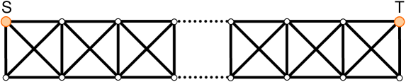
This architecture, displayed in Fig. 1, is constituted by the repetition of perfect graphs (the fully-connected graph with four nodes). This configuration is exactly solvable even when edges and nodes have distinct reliabilities [6]. For perfect nodes, and with all edge reliabilities equal to , the two-terminal reliability has the simple form
| (20) | |||||
| (21) | |||||
| (22) | |||||
| (23) |
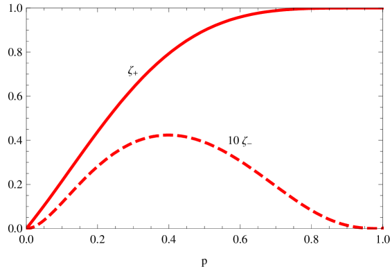
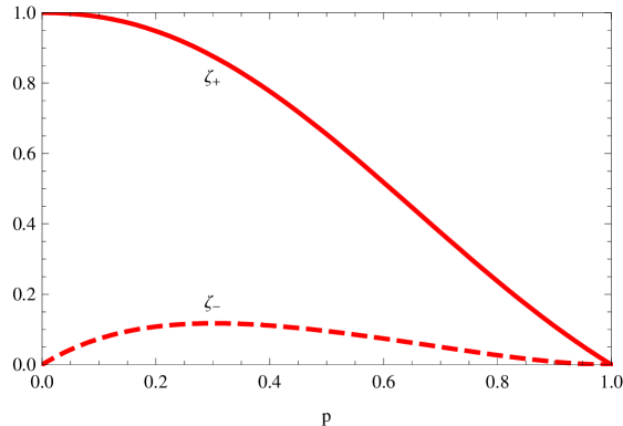
The two eigenvalues are displayed in Fig. 2 as functions of . As increases, the contribution of prevails over that of . Therefore, when is large,
| (24) |
because the contribution of vanishes exponentially. The approximation given by eq. (24) lies at the heart of our method for deriving the MTTF’s asymptotic expansion. Inserting it into eq. (10) gives
| (25) |
Here, the lower bound (zero) does not play a significant role because . As increases, is negligible except close to , as illustrated in Fig. 3.
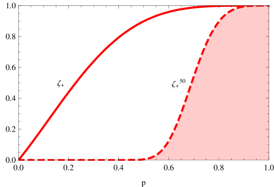
The gist of the asymptotic expansion is therefore to consider and in the vicinity of unity. Setting , we have from eqs. (21)–(22)
| (26) | |||||
| (27) |
Note that because . We can write
| (28) |
At this point, we have to rescale the variable in order to extract the asymptotic behavior of the integral. Equation (27) gives
| (29) |
this suggests setting , or equivalently , so that
| (30) |
In the last exponential, the argument is . Because of the factor, we can neglect the contribution of large ’s, so that when is large, we only need to expand the second exponential and all other factors in the limit :
| (31) |
The error made by replacing the upper bound of the integral by vanishes exponentially as goes to infinity. Keeping only the prevailing terms in each factor of eq. (31) leads to
| (32) | |||||
For the leading-order term (and this term only), does not play any role since it may safely be replaced with 1. The asymptotic -dependence is not or anymore as in the series and parallel cases, but a power-law, , which slowly decreases with . The following terms of the expansion may be derived easily by expanding all the factors in eq. (31):
| (33) |
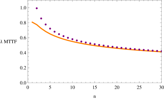
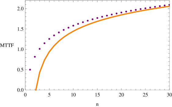
The exact MTTF is obtained straightforwardly by using eq. (10) and the value deduced from the three-term recursion relation at the origin of eq. (20):
| (34) | |||||
with and . The exact values of the MTTF are then obtained by a simple integration of . The exact and the asymptotic (limited to the first three terms of the expansion) results for the MTTF are plotted in Fig. 4. Even for moderate values of , the agreement between the two is good.
Following this method, we also find the asymptotic expansion of by adding the factor and another in eq. (31). As regards the leading term of the expansion, a mere factor is added in the integral. Finally
| (35) |
Further terms can be routinely obtained using mathematical software such as Mathematica.
After simplification, the variance of the distribution is therefore deduced to behave as
| (36) |
We could perform similar calculations for higher moments or cumulants, and again would find asymptotic power-law behaviors.
3.2 Generalized fan
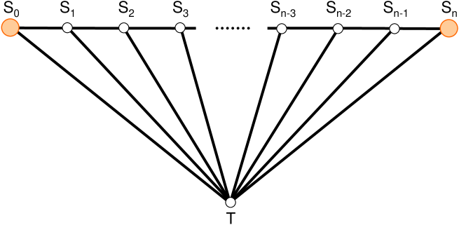
This architecture, displayed in Fig. 5, has been considered in previous studies [11, 12, 13] and recently solved for the two-terminal reliability between and [5]. For perfect nodes,
| (37) |
When , clearly tends to the constant ( is always less than 1/4, so the last contribution in eq. (37) decreases faster than ). This stems from the existence of one path with a finite number of hops, namely . The MTTF’s asymptotic behavior is therefore different from that of the preceding section: it does not vary with . This is also true for higher moments, with
| (38) |
where . The first of these integrals are
| (39) | |||||
| (40) |
where is the derivative of the digamma function . From the first values of , we can infer the general result
| (41) | |||||
Depending on the parity of , the difference may actually be further simplified (leaving only for even, or powers of for odd). It is easy to prove that, asymptotically,
| (42) |
In that limit, it looks as if only the connection exists.
3.3 Double fan
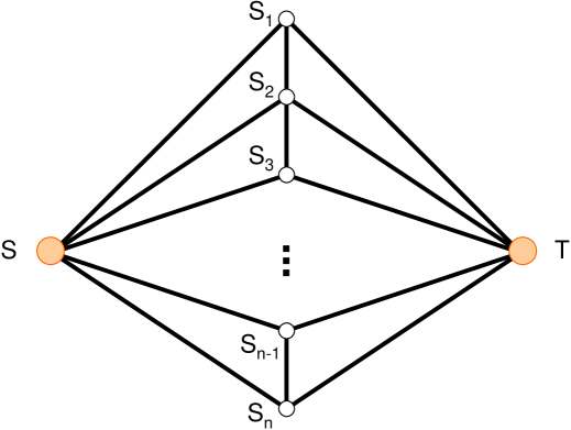
This configuration, displayed in Fig. 6, is a slight generalization of double links in parallel. As , there is an infinity of paths of finite length connecting to ; for perfect nodes, the associated two-terminal reliability is [7]
| (43) |
with
| (44) | |||||
| (45) |
Here again — if we forget that 1 is a third eigenvalue – we have two eigenvalues . However, the situation is different from that of the ladder, because when , while and when . We also expect that
| (46) |
the right-hand side of eq. (46) corresponding to elements of reliability in parallel.
As increases, the contribution of prevails over that of (see Fig. 7), so that . Consequently,
| (47) |
Because of the factor, the asymptotic expansion of is now controlled by the behaviors of and for :
| (48) | |||||
| (49) |
We can write
| (50) | |||||
Each term on the right-hand side of eq. (50) vanishes for , so that the factor does not lead to a diverging integral in eq. (47). The first term of eq. (50) gives the prevailing contribution, namely
| (51) | |||||
This contribution is — unsurprisingly — half the usual result for elements in parallel, because the reliability translates into a failure rate. For the two other contributions, the change of variable gives a factor ; the remaining factors in eq. (50) must be expanded in the vicinity of , as in section 3.1. Summing the three contributions gives
| (52) |
A comparison of the exact results with the asymptotic expansion in which we have kept the first three terms of eq. (52) is plotted in Fig. 8. The agreement is good, even for moderate values of .
3.4 Street
In the preceding subsections, we have considered architectures for which is exactly known through the analytic expressions of two eigenvalues . In complex systems, more than two eigenvalues may coexist, and be known only as roots of polynomial equations. However, the MTTF’s asymptotic expression can still be derived from the knowledge of the generating function [14] of the ’s, namely
| (53) |
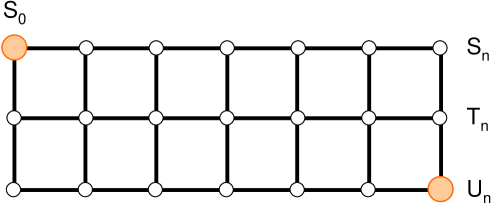
Such is the case of the Street , displayed in Fig. 9. This configuration has been studied for the two-terminal reliability between and [6, 15, 16, 17, 18, 19, 20, 21] (there is actually an offset of 1 between our and these references’ because our source is ). For perfect nodes, is given by , with [6]
| (54) | |||||
| (55) | |||||
| (56) | |||||
, and are polynomials in both and .
The eigenvalue of greatest modulus, named again, actually obeys for (in the limit , and ); all other eigenvalues tend to zero in that limit. Even though it is not possible to get an analytic expression for as a function of ( is of degree 6 in ), we can readily compute it numerically. We can also deduce from the constraint the expansion of as a function of for small ’s, starting with :
| (57) | |||||
| (58) |
The scaling variable should be times the leading term of eq. (58), namely , so that
| (59) | |||||
is deduced from and the numerical value of through the residue of at . The general result is
| (60) |
where is the denominator of and . Here, , leading to
| (61) |
After inserting eqs. (59) and (61) in eq. (29), and further series expansions and integration similar to those of Section 3.1, the final asymptotic expansion reads
| (62) |
Here again, it exhibits a power-law behavior, but this time. In the next section, we relate the exponent to a specific property of the network.
4 General case
In the preceding section, we have derived the asymptotic MTTF when the two-terminal reliability is known, at least implicitly through a recursion relation. Here, we want to show that the leading terms of the MTTF and other moments may be obtained for arbitrary, recursive configurations. As shown in [6], can be generally expressed as a product of transfer matrices — whose size may be large but remains finite. For identical edge reliabilities , the asymptotic behavior is controlled by the largest eigenvalue of the (now unique) transfer matrix. We consider in the following architectures that look like some kind of “series-like” system, albeit more complex than those of the ladder and the Street , or to a “parallel-like” one, like the double fan.
4.1 “Series-like” configuration
This happens when the shortest path connecting the source to the destination has a length equivalent to as . Here, we use again , and the MTTF is still controlled by the behavior of and in the vicinity of . The relevant expansions for have the form
| (63) | |||||
| (64) |
from which
| (65) |
The adequate change of variable is now , or equivalently ; the upper bound of the integral, , may again be replaced by . The first term in the asymptotic expansion is therefore
| (66) | |||||
Likewise, in order to calculate the first term of the asymptotic expansion of , we have an additional factor , which is equivalent to when and brings an extra . Finally,
| (67) |
so that the variance goes as
| (68) |
from which
| (69) |
which is independent of . Actually, it only depends on , which is the lowest order of the -dependence of when (see eq. (63)).
For the higher moments , the generalization is straightforward; we can also go beyond the first order in the expansion, following the recipe of the preceding section. Setting , we find
| (70) | |||||
We may wonder: is this result merely formal, or is it actually possible to determine for an arbitrary, recursive network ? The answer to this question is yes. Even though we do not know the exact value of or the associated greatest eigenvalue , we can still infer the ’s and ’s appearing in eqs. (63)–(64) because for large , . These parameters can be deduced from the expansion of the unavailability for . We have
| (71) | |||||
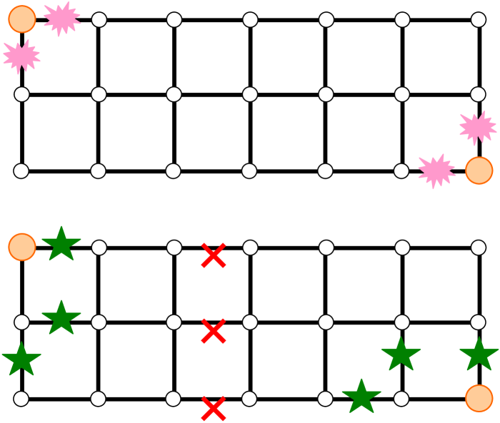
and must keep track of the successive powers of , along with their dependence with . Let us illustrate this claim with the Street case. A simple cut enumeration gives (when is large, so as to avoid “boundary” effects)
| (72) |
The first term of the right-hand side of eq. (72) is easy to obtain. There are only two cuts of order 2 preventing a connection between source and destination (see the top of Fig. 10), hence the term. For the cuts of order 3, different possibilities occur as displayed at the bottom of Fig. 10. Firstly, three parallel links may fail; there are such instances. Secondly, close to the source or the destination, there are four triple failures (only two are represented by green stars in Fig. 10, the remaining ones can be deduced by symmetry). This gives the term. A comparison between eqs. (71) and (72) gives , , , and . From these values, we get
| (73) |
which agrees with eq. (62) when .
In conclusion, the exponent of the power-law behavior in is nothing but the inverse of the number of necessary cuts to isolate each elementary cell from its neighbors. Note that is not necessarily equal to 1, since it represents the number of independent cuts of order .
4.2 “Parallel-like” configuration
We can also consider configurations where the reliability is asymptotically equal to 1 when , as in section 3.3. In the vicinity of (the relevant domain here), and the needed expansions are
| (74) | |||||
| (75) |
so that
| (76) |
The contribution of A is (omitting the factor)
| (77) |
The contribution of B depends on the value of because
| (78) |
If , we must take the two terms of degree 2 into account; otherwise, only the term needs be kept. After asymptotic expansions similar to those performed in the preceding sections, we have
| (79) | |||||
| (80) |
The contribution of C is easier to compute because vanishes as , thereby compensating the singular term in the integral. With the change of variable , we get
| (81) |
Note that the -dependence of C is , which decreases less rapidly than if . The sum of contributions A, B, and C finally expands as (for )
| (82) |
As in the preceding subsection 4.1, the coefficients , , etc. may be deduced by evaluating the availability through a path enumeration in the limit . For instance, in the case of the double fan
| (83) |
This must be compatible with the expansions of and in eqs. (74)–(75). Because eq. (83) has no linear term, . The coefficient of being equal to , we deduce , , and ; the coefficient of then implies . Inserting these values in eq. (82) gives back the first two terms of eq. (52).
5 Approximate reliability of large, recursive, “series-like” systems
We have seen that the asymptotic expansion of the MTTF and the higher moments for a large, recursive system can be obtained with minimal effort. In the same line of thought, is it possible to find an approximate reliability such that all its moments give the same value as the true reliability, at least for the first terms of the expansion in . The first term of eq. (70), namely
| (84) |
reminds us of what would be obtained for a Weibull distribution [1, 3]. Indeed, it is straightforward to show that
| (85) |
would give eq. (84) exactly.
Is it possible to improve this expression, i.e., propose an effective reliability leading to the correct first two terms in the asymptotic expansion of each moment ? Provided that , i.e., that there is no cut of order one (it would then be easy to factor out this link contribution, and proceed with the remaining parts of the system), the answer is again positive.
Calculating the moments of
| (86) |
we find that
| (87) |
Equations (70) and (87) match if
| (88) |
so that for , the constraint is satisfied when
| (89) |
This finally gives
| (90) |
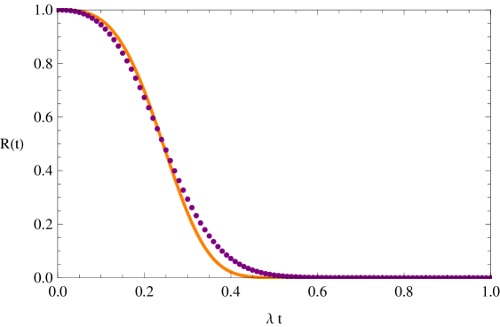
This expression slightly improves over the Weibull distribution of eq. (85). In the case of the Street ,
| (91) |
This expression and the true reliability are plotted in Fig. 11; the agreement is already satisfying for .
6 Non-exponential distribution functions
In the preceding sections, we have considered elements whose reliability is . Although this distribution is often chosen because calculations are simpler, other models may be used: Weibull, gamma, lognormal, etc. [1, 3]. We investigate here the influence of the true on the -dependence of the MTTF and higher moments for “series-like” systems.
For “series-like” configurations, we have again to consider what happens for , or equivalently for . Assuming that asymptotically
| (94) |
we have (because )
| (95) |
so that
| (96) |
Keeping and , we get to lowest order
| (97) | |||||
The -dependence of is therefore affected by the structure of the graph (through and ) and by the true failure-time distribution of each element (through and ). The exponent of the power-law asymptotic behavior is , and the total reliability goes asymptotically as
| (98) |
7 Conclusion
We have shown that very simple asymptotic expansions may be obtained for the mean time to failure (and higher moments) for general recursive, meshed networks. By contrast with the simple series and parallel systems considered in many textbooks, the size-dependence of the MTTF of a “series-like” system follows a power-law behavior, whose exponent is linked to the number of cuts disconnecting an elementary cell to its neighbors. Comparison with the exact results for various architectures show that the agreement is often reached when the system contains a few dozens of the (repeated) pattern structure. A simple, approximate expression for the effective global reliability of the system has also been proposed, which is very simple to derive by a mere enumeration of cut-sets or path-sets.
The calculations have been performed in the context of the two-terminal reliability of general systems; they obviously apply to all-terminal reliability, and would belong to the “series-like” category.
Acknowledgment
Useful and stimulating discussions with Nancy Perrot, Guillaume Boulmier, Matthieu Chardy, Bertrand Decocq, Sébastien Nicaisse, and Mathieu Trampont are gratefully acknowledged.
References
- [1] Shooman ML. Probabilistic reliability: an engineering approach. New York: McGraw-Hill; 1968.
- [2] Singh C, Billinton R. System reliability modelling and evaluation. London: Hutchinson; 1977.
- [3] Kuo W, Zuo MJ. Optimal Reliability Modeling: Principles and Applications. Hoboken: Wiley, 2003.
- [4] Tanguy C. Exact solutions for the two- and all-terminal reliabilities of a simple ladder network. arXiv:cs.PF/0612143.
- [5] Tanguy C. Exact solutions for the two- and all-terminal reliabilities of the Brecht-Colbourn ladder and the generalized fan. arXiv:cs.PF/0701005.
- [6] Tanguy C. What is the probability of connecting two points ? J Phys A: Math Theor 2007;40:14099?14116.
- [7] Tanguy C. Exact two-terminal reliability for the double fan. In: Proc of the International Network Optimization Conference 2007 (INOC’07).
- [8] Kołowrocki K. Reliability of Large Systems. Amsterdam: Elsevier; 2004.
- [9] Gradshteyn IS, Ryzhik IM. Table of Integrals, Series, and Products. 5th edition, editor Jeffrey A. New York: Academic Press; 1994.
- [10] Patel JK, Kapadia CH, Owen DB. Handbook of Statistical Distributions. New York: Marcel Dekkar; 1976.
- [11] Aggarwal KK, Gupta JS, Misra KB. A simple method for reliability evaluation of a communication system. IEEE Trans Communications 1975; 23:563?566.
- [12] Neufeld EM, Colbourn CJ. The most reliable series-parallel networks. Networks 1985;15:27?32.
- [13] Gordon G, McMahon E. A characteristic polynomial for rooted graphs and rooted digraphs. Discr Math 2001;232:19?33.
- [14] Stanley RP. Enumerative combinatorics, vol 1, chap 4. Cambridge: Cambridge University Press; 1997.
- [15] Theologou OR, Carlier JG. Factoring & reductions for networks with imperfect vertices. IEEE Trans Reliability 1991;40:210?217.
- [16] Carlier J, Lucet C. A decomposition algorithm for network reliability evaluation. Discr Appl Math 1996;65:141?156.
- [17] Kuo S, Lu S, Yeh F. Determining terminal pair reliability based on edge expansion diagrams using OBDD. IEEE Trans Reliability 1999;48(3):234?246.
- [18] Yeh FM, Lu SK, Kuo SY. OBDD-based evaluation of k-terminal network reliability. IEEE Trans Reliability 2002;51(4):443?451.
- [19] Yeh FM, Lin HY, Kuo SY. Analyzing network reliability with imperfect nodes using OBDD. In: Proc of the 2002 Pacific Rim International Symposium on Dependable Computing (PRDC’02), p. 89–96.
- [20] Rauzy A. A new methodology to handle Boolean models with loops. IEEE Trans Reliability 2003;52(1):96?105.
- [21] Hardy G, Lucet C, Limnios N. K-Terminal Network Reliability Measures With Binary Decision Diagrams. IEEE Trans Reliability 2007;56(3):506?515.