Asymptotic-preserving schemes for kinetic-fluid modeling of mixture flows with distinct particle sizes

Shi Jin shijin-m@sjtu.edu.cn School of Mathematical Sciences, Shanghai Jiao Tong University, Shanghai200240, China Institute of Natural Sciences, Shanghai Jiao Tong University, Shanghai200240, China Ministry of Education, Key Laboratory in Scientific and Engineering Computing, Shanghai Jiao Tong University, Shanghai200240, China Yiwen Lin linyiwen@sjtu.edu.cn

Abstract

We consider coupled models for particulate flows, where the disperse phase is made of particles with distinct sizes. We are thus led to a system coupling the incompressible Navier–Stokes equations to the multi-component Vlasov–Fokker–Planck equations. We design an asymptotic-preserving numerical scheme to approximate the system. The scheme is based on suitable implicit treatment of the stiff drag force term as well as the Fokker–Planck operator, and can be formally shown to capture the hydrodynamic limit with time step and mesh size independent of the Stokes number. Numerical examples illustrate the accuracy and asymptotic behavior of the scheme, with several interesting applications.

keywords:

particulate flows , coupled kinetic-fluid model , Vlasov-Fokker-Planck-Navier-Stokes equations , asymptotic preserving schemes

1 Introduction

This paper concerns the kinetic-fluid models for a mixture of flows in which the particles represent the disperse phase evolving in a dense fluid. Applications of such kinetic-fluid models include the dispersion of smoke or dust [14], biomedical modeling of spray [3], coupled models in combustion theory [36], etc. Specifically, we focus on the models that describe a large number of particles, with distinct but fixed sizes, interacting with a fluid. Here the dense fluid phase is modeled by the Euler or Navier-Stokes equations and particles dispersed in the fluid are modeled by Fokker-Planck type kinetic equations. Such multi-size particle systems have a wide range of applications in engineering, especially for the complex meteorological simulation of large aircraft icing process. For the distribution of droplets in the air, the influence of large droplets contained in the droplet distribution cannot be ignored [12, 22, 34]. However, it is very difficult to simulate multi-size particles by experimental means. See [35, 20] for more details on the modeling of such multi-phase flows.

In this paper, we study the model where the evolution of the particle distribution function is driven by a combination of particle transport, a drag force exerted by the surrounding fluid on the particle obeying the Stokes Law, an external force field (such as gravity, electrostatic force, centrifugal force, etc.) and Brownian motion of particles. For the two physically important regimes first investigated by Goudon et al. [16, 17], we focus on the fine particle regime given in [17]. The fluid phase is incompressible and viscous, all phases are isothermal, with interactions including coagulation and fragmentation that occur between particles, while the change of particle sizes is ignored. For the sake of simplicity, we suppose that the fluid density is constant and homogeneous. In this model, particles and fluid systems are coupled through nonlinear terms. Such a coupling and nonlinearities pose new difficulties in mathematical analysis and numerical computations when compared with uncoupled problems. Furthermore, from a numerical point of view, the kinetic framework leads to high computational costs in both size and time, posing further computational challenges.

The study of existence, uniqueness and regularity problems depends on the nature of the coupling and the complexity of the equations used to describe the fluid. For the two-phase flow model system, it is worth mentioning related works like existence of strong solutions locally in time without velocity-diffusion [4], existence of weak solutions for the Vlasov–Stokes system [21] and for the incompressible Vlasov–Navier–Stokes system on a periodic domain [6] or a bounded domain [37], global-in-time existence of classical solutions close to the equilibrium for the incompressible Navier–Stokes–Vlasov–Fokker–Planck system [15], analysis of compressible models [30], several studies of coupling with the Euler system without viscosity [9, 7] and systems with energy exchanges [5]. Analysis of the asymptotics in the two-phase flow system is due to [16, 17] by means of relative entropy methods, see also [31]. For the multi-phase flow model system (2.1), existence has been discussed in [20] and regularity properties of the solutions close to the equilibrium as well as its long time behavior have been investigated recently by the authors in [27].

Numerical methods for such particulate flows have been developed in recent years, including particle-in-cell method [1], Eulerian–Lagrangian method [33, 32], level set approach [29] and so on. One of the difficulties in numerically solving such multi-component Vlasov-Fokker-Planck-Navier-Stokes systems comes from the varying Stokes number $\varepsilon$ , which describes the ratio of the Stokes settling time over a certain time unit of observation. Due to the multiscale nature of the problem, it is often desired to design numerical schemes that possess the asymptotic-preserving (AP) properties [8, 19, 18]. The AP schemes (coined in [23]) refer to those that, when letting the Stoeks number $\varepsilon$ go to zero and holding the mesh size and time step fixed, the numerical schemes for coupled kinetic-fluid models automatically become good numerical schemes for the hydrodynamic limiting equations, with numerical stability independent of $\varepsilon$ . We refer to [24, 25] and references therein for reviews on AP schemes and their applications. Most of these references do not address the effect of different particle sizes, namely all particles in the model are assumed to be in the same size. This paper considers kinetic-fluid models for a mixture of the flows for particles with distinct sizes.

The goal of this work is to design a numerical scheme to simulate the behavior of the fluid-particles systems with disparate particle sizes, capable of handling different regimes, from $\varepsilon=O(1)$ (the kinetic regime) to $\varepsilon\ll 1$ (the hydrodynamic regime). We will follow the discretization introduced in [28]. Specifically, the AP scheme for this multi-phase model uses a combination of the projection method [10, 11] for the Navier-Stokes equations and an implicit treatment for stiff Fokker-Planck operators. In addition to the challenge of nonlinear coupling between particles and the fluid, new difficulty arises here due to the multi-phase properties where the disperse phase is made of particles with distinct sizes. Roughly speaking, one needs to prove the velocities of different species equilibrate which is a property one does not encounter for two-phase kinetic-fluid systems with identical particle size, and thus one has to investigate different convergence rates to equilibria for particles with different sizes and to justify AP properties of the scheme under the multi-phase kinetic-fluid system with disparate particle sizes. For the coupling and nonlinearities, the construction of the scheme relies on evaluating implicitly the stiff terms of the multi-phase system. It will require a carefully-designed time splitting which allows to compute implicitly the stiff drag force term efficiently and an inversion of the Fokker-Planck operator. In the hydrodynamic regime, the particle distribution function relaxes to the Maxwellian and the limiting system for particle density $n$ and particle macroscopic velocity $u$ , which coincides to the fluid velocity, looks like a variable density incompressible Navier-Stokes system, see (2.7). This justifies the asymptotic-preserving property of the scheme, which has a much relaxed numerical stability condition than a non-AP discretization, and can capture the hydrodynamic limit with time step and mesh size independent of the Stokes number.

The paper is organized as follows. In Section 2, we detail some basic facts about the PDE system of interest to us, including its hydrodynamic limit system ( $\varepsilon\rightarrow 0$ ). In Section 3, we give the details of the numerical scheme. Both first-order and second-order schemes are presented in this framework and the AP property will be studied. Section 4 is devoted to numerical simulation for checking accuracy, asymptotic behavior, and some applications, followed by conclusions in Section 5.

2 A Model Problem

In this paper, we focus on the fine particle regime, in which the suitably scaled PDE systems for the multi-phase model are given by [27]:

\left\{\begin{aligned} &\begin{aligned} (f_{i})_{t}+v\cdot\nabla_{x}(f_{i})-\nabla_{x}\Phi\cdot\nabla_{v}f_{i}&=\dfrac{1}{\varepsilon}\dfrac{1}{i^{2/3}}\mathcal{L}_{u,i}f_{i},(t,x,v)\in\mathbb{R}^{+}\times\mathbb{T}^{3}\times\mathbb{R}^{3},i=1,2,...,N,\end{aligned}\\ &u_{t}+\nabla_{x}\cdot(u\otimes u)+\nabla_{x}p-\dfrac{1}{Re}\Delta_{x}u=\dfrac{\kappa}{\varepsilon}\sum_{i=1}^{N}\int_{\mathbb{R}^{3}}(v-u)f_{i}i^{1/3}\mbox{d}v,\quad(t,x)\in\mathbb{R}^{+}\times\mathbb{T}^{3},\\ &\nabla_{x}\cdot u=0,\end{aligned}\right.

(2.1)

with the initial condition

\left.u\right|_{t=0}=u_{0},\quad\nabla_{x}\cdot u_{0}=0,\left.\quad f_{i}\right|_{t=0}=f_{i,0},

where $\mathcal{L}_{u,i}f_{i}$ is the $i$ th Fokker-Planck (FP) operator

\mathcal{L}_{u,i}f_{i}=\nabla_{v}\cdot\left((v-u)f_{i}+\dfrac{\bar{\theta}}{i}\nabla_{v}f_{i}\right),\ i=1,2,\ldots,N,

with $N$ the number of particle sizes. Without loss of generality, assume the reference temperature $\bar{\theta}=1$ throughout the paper. The discussion of the scaling issues is detailed in Appendix. Here $t\geq 0$ is time, $x=\left(x_{1},x_{2}\right)\in\Omega\subset\mathbb{R}^{2}$ is the space variable, and $v=\left(v_{1},v_{2}\right)\in\mathbb{R}^{2}$ is the particle velocity. $f_{i}=f_{i}(t,x,v),i=1,2,\ldots,N$ are the density functions of the particles. $u=u(t,x)=\left(u_{1}(t,x),u_{2}(t,x)\right)$ is the velocity field of the fluid. $\Phi=\Phi(x)$ is an external force field and $\nabla_{x}\Phi$ represents the effect of the external force field on the particles. The first equation describes the motion of particles. The two terms in the Fokker-Planck (FP) operator come from the drag force from the fluid and the effect of Brownian motions, respectively. The second and third equations are the standard incompressible Navier-Stokes equations for the fluid, with the right-hand-side term describing the force coming from the particles. $\kappa>0$ is the coupling constant, which equals the ratio between the particle density $\rho_{P}$ and fluid density $\rho_{F}$ , and $Re$ is the Reynolds number. $\varepsilon$ $(0<\varepsilon\leq 1)$ is the Stokes number given by $\varepsilon=\frac{2\rho_{p}i^{2}}{9\mu}$ , with $\mu$ the dynamic viscosity of the fluid, $i$ the typical radius of the particles and $\rho_{P}$ the density of the particles. Here $\varepsilon$ is a constant with $i=1$ . Its correlation with the particle size $i$ is given explicitly in the Eq. 2.1. $\varepsilon=O(1)$ corresponds to the kinetic regime, while $\varepsilon\rightarrow 0$ corresponds to the fluid regime. $Re$ is the Renalds number.

Let us briefly recall some basic facts about system (2.1) and the regime $\varepsilon\rightarrow 0$ . The key remark, observed in [16, 17], is the following energy-entropy dissipation property

	$\displaystyle\frac{\mathrm{d}}{\mathrm{d}t}\left(\kappa\sum_{i=1}^{N}\int_{\mathbb{T}^{3}}\int_{\mathbb{R}^{3}}f_{i}\left(\ln(f_{i})+1+i\Phi+i\frac{\|v\|^{2}}{2}\right)\,\mathrm{d}v\mathrm{d}x+\int_{\mathbb{T}^{3}}\frac{\|\tilde{u}\|^{2}}{2}\,\mathrm{d}x\right)+\int_{\mathbb{T}^{3}}\left\|\nabla_{x}\tilde{u}\right\|^{2}\,\mathrm{d}x$		(2.2)
	$\displaystyle+\frac{\kappa}{\varepsilon}\sum_{i=1}^{N}\int_{\mathbb{T}^{3}}\int_{\mathbb{R}^{3}}\left\|(v-\tilde{u})\sqrt{i^{1/3}f_{i}}+\frac{\bar{\theta}\nabla_{v}f_{i}}{\sqrt{i^{5/3}f_{i}}}\right\|^{2}\,\mathrm{d}v\mathrm{d}x=0.$		(2.2)

A similar relation holds when the problem is set on a bounded smooth domain $\Omega$ with reasonable boundary conditions. For instance one can assume no-slip of the fluid

\left.u\right|_{\partial\Omega}=0

and specular reflection of the particles

\gamma^{-}f_{i}(t,x,v)=\gamma^{+}f_{i}(t,x,v-2v\cdot\hat{v}(x)\hat{v}(x)),

where $\hat{v}(x)$ stands for the unit outer normal at point $x\in\partial\Omega$ and $\gamma^{\pm}$ denote the trace operators on the set

\left\{(t,x,v)\in(0,\infty)\times\partial\Omega\times\mathbb{R}^{2},\quad\pm v\cdot\hat{v}(x)>0\right\}.

We refer to further comments in [9]. It is worth rewriting the Fokker-Planck operator as

L_{u,i}f_{i}=\frac{1}{i}\nabla_{v}\cdot\left(M_{u,i}\nabla_{v}\left(\frac{f_{i}}{M_{u,i}}\right)\right),\quad M_{i,u}(v)=\frac{i}{2\pi}\exp\left(-\frac{i|v-u(t,x)|^{2}}{2}\right).

As $\varepsilon$ goes to $0$ , since the Fokker-Planck operator is penalized and the change of particles sizes is ignored, we expect that $f_{i}$ makes $L_{u,i}f_{i}$ (and the dissipation term in (2.2)) vanish which means that $f_{i}$ becomes proportional to the Maxwellian centered on the fluid velocity

f_{i}(t,x,v)\simeq n_{i}(t,x)M_{i,u(t,x)}.

Hence the question is to identify the equation satisfied as $\varepsilon\rightarrow 0$ by the particles density $n$ and the velocity $u$ .

For the deterministic multi-size particle-fluid systems (2.1), we associate to $f_{i}(t,x,v),i=1,2,\ldots,N$ the following macroscopic quantities:

\begin{gathered}n_{i}(t,x)=\int_{\mathbb{R}^{3}}f_{i}(t,x,v)\mathrm{d}v,\quad\rho_{i}(t,x)=in_{i}(t,x),\quad J_{i}(t,x)=i\int_{\mathbb{R}^{3}}vf_{i}(t,x,v)\mathrm{d}v,\\ \mathbb{P}_{i}(t,x)=i\int_{\mathbb{R}^{3}}v\otimes vf_{i}(t,x,v)\mathrm{d}v,\end{gathered}

where $\rho_{i},J_{i}$ and $\mathbb{P}_{i}$ are the mass, momentum and stress tensors, respectively, of particles of size $i$ . Integrating the first equation in (2.1) with respect to $i\mathrm{~{}d}v$ and $iv\mathrm{~{}d}v$ respectively, one obtains

i\partial_{t}n_{i}+\nabla_{x}\cdot J_{i}=0,

(2.3)

and

\partial_{t}(J_{i})+\operatorname{Div}_{x}(\mathbb{P}_{i})+in_{i}\nabla_{x}\Phi=-\frac{1}{i^{2/3}\varepsilon}\left(J_{i}-in_{i}u\right).

(2.4)

Combined to system (2.1), one has

\begin{array}[]{r}\partial_{t}\left(u+\kappa\displaystyle\sum_{i=1}^{N}(J_{i})\right)+\operatorname{Div}_{x}\left(u\otimes u+\kappa\displaystyle\sum_{i=1}^{N}(\mathbb{P}_{i})\right)+\nabla_{x}p\\ +\kappa\displaystyle\sum_{i=1}^{N}(in_{i})\nabla_{x}\Phi-\dfrac{1}{Re}\Delta_{x}u=0.\end{array}

(2.5)

Accordingly, for $\varepsilon<<1$ , $J_{i}$ and $\mathbb{P}_{i}$ are asymptotically defined by the moments of the Maxwellian, i.e.,

J_{i}\simeq in_{i}u,\quad\mathbb{P}_{i}\simeq in_{i}u\otimes u+in_{i}\mathbb{I}.

Inserting this ansatz into (2.5), one arrives at

	$\displaystyle\partial_{t}\left(\left(1+\kappa\sum_{i=1}^{N}in_{i}\right)u\right)+\operatorname{Div}_{x}\left(\left(1+\kappa\sum_{i=1}^{N}in_{i}\right)u\otimes u\right)+\nabla_{x}\left(p+\kappa\sum_{i=1}^{N}in_{i}\right)$			(2.6)
	$\displaystyle+\kappa\sum_{i=1}^{N}(in_{i})\nabla_{x}\Phi-\frac{1}{Re}\Delta_{x}u=0,$			(2.6)

Denote $\nu=\displaystyle\sum_{i=1}^{N}in_{i}$ with $n_{i}(t,x)=\int_{\mathbb{R}^{3}}f_{i}(t,x,v)\mathrm{d}v$ . As $\varepsilon\rightarrow 0$ , (2.1) has a hydrodynamic limit

\left\{\begin{aligned} &\partial_{t}\nu+\nabla_{x}\cdot(\nu u)=0,\\ &\partial_{t}\left(\left(1+\kappa\nu\right)u\right)+\operatorname{Div}_{x}\left(\left(1+\kappa\nu\right)u\otimes u\right)+\nabla_{x}\left(p+\kappa\nu\right)+\kappa\nu\nabla_{x}\Phi-\frac{1}{Re}\Delta_{x}u=0,\\ &\nabla_{x}\cdot u=0,\end{aligned}\right.

(2.7)

which is an incompressible Navier-Stokes system for the composite and inhomogeneous density $(1+\kappa\nu)$ .

In this paper, we are interested in numerical approximations of system (2.1). We will pay particular attention to the scaling parameter $\varepsilon$ : the scheme should work over a wide range of values of the parameter, capturing the expected asymptotic behavior without introducing restrictions that would make small $\varepsilon$ ’s simulations numerically prohibitive. This scheme consists in discretizing implicitly the stiff terms in the equations, but it should be done as simple as possible because the inversion of the corresponding discrete system will be the main source of numerical cost.

The scheme we developed can automatically capture the hydrodynamic limit (2.7) as $\varepsilon\rightarrow 0$ . This is the so-called Asymptotic Preserving (AP) property, a term first introduced by Jin [23]. The AP scheme is effective in the hydrodynamic regime ( $\varepsilon\ll 1$ ) because it allows capturing the hydrodynamic limit (2.7) without numerically resolving the small scale $\varepsilon$ . We refer to [24, 25] for reviews on AP schemes and their applications.

3 An AP Scheme for Multi-phase Flows

We now give the details to update the numerical unknowns, having at hand $u^{k},p^{k},f_{i}^{k}$ and thus

n_{i}^{k}=\int_{\mathbb{R}^{d}}f_{i}^{k}\mathrm{d}v,\quad J_{i}^{k}=i\int_{\mathbb{R}^{d}}vf_{i}^{k}\mathrm{d}v,\quad i=1,2,...,N.

3.1 The time discretization - first order

Step 1. Advancing densities. Compute $n_{i}^{k+1}$ .

\displaystyle\dfrac{1}{\Delta t}\left(n_{i}^{k+1}-n_{i}^{k}\right)

\displaystyle=-\int v\cdot\nabla_{x}f_{i}^{k}\mathrm{~{}d}v

(3.1)

Step 2. Pressureless step. Compute $u^{*},J_{i}^{*}$ .

Notice that in order to derive an AP scheme, one has to impose the stiff drag force term in both the viscosity step and the projection step.

Solve the viscosity part of momentum equations with only part of the stiff term:

		$\displaystyle\dfrac{1}{\Delta t}\left(J_{i}^{}-J_{i}^{k}\right)=-i\int v\otimes v\nabla_{x}f_{i}^{k}\mathrm{~{}d}v-in_{i}^{k}\nabla_{x}\Phi-\dfrac{1-\alpha}{i^{2/3}\varepsilon}\left(J_{i}^{}-in_{i}^{k+1}u^{*}\right),$		(3.2)
		$\displaystyle\dfrac{1}{\Delta t}\left(u^{}-u^{k}\right)-\dfrac{1}{Re}\Delta_{x}u^{}=-\nabla_{x}\cdot\left(u^{k}\otimes u^{k}\right)+\sum_{i=1}^{N}\dfrac{(1-\alpha)\rho_{P}}{i^{2/3}\varepsilon\rho_{F}}\left(J_{i}^{}-in_{i}^{k+1}u^{}\right),$		(3.2)

where $\alpha\in(0,1)$ is any constant. One can simply choose $\alpha=\dfrac{1}{2}$ .

Eliminating $J_{i}^{*}$ , and with the no-slip boundary condition for $u^{*}$ used, one obtains a Helmholtz equation for $u^{*}$ :

\left\{\begin{array}[]{l}\begin{aligned} &\left(\dfrac{1}{\Delta t}+\sum_{i=1}^{N}\dfrac{(1-\alpha)\rho_{P}}{(i^{2/3}\varepsilon+(1-\alpha)\Delta t)\rho_{F}}in_{i}^{k+1}-\dfrac{1}{Re}\Delta_{x}\right)u^{*}\\ &=\dfrac{u^{k}}{\Delta t}-\nabla_{x}\cdot\left(u^{k}\otimes u^{k}\right)+\sum_{i=1}^{N}\dfrac{(1-\alpha)\rho_{P}}{(i^{2/3}\varepsilon+(1-\alpha)\Delta t)\rho_{F}}\left(J_{i}^{k}-i\Delta t\int v\otimes v\nabla_{x}f_{i}^{k}\mathrm{~{}d}v-i\Delta tn_{i}^{k}\nabla_{x}\Phi\right)\end{aligned}\\ \left.u^{*}\right|_{\partial\Omega}=0\end{array}\right.

(3.3)

$u^{*}$ can be solved by the Preconditioned Counugate Gradient method and then $J_{i}^{*}$ can be solved accordingly from (3.2).

Step 3. Projection step. Compute $p^{k+1},u^{k+1}$ .

Next $u^{*}$ is projected to the divergence free space, with the remaining stiff coupling term:

		$\displaystyle\dfrac{1}{\Delta t}\left(J_{i}^{*}-J_{i}^{}\right)=-\dfrac{\alpha}{i^{2/3}\varepsilon}\left(J_{i}^{**}-in_{i}^{k+1}u^{k+1}\right)$		(3.4)
		$\displaystyle\dfrac{1}{\Delta t}\left(u^{k+1}-u^{}\right)+\nabla_{x}p^{k+1}=\sum_{i=1}^{N}\dfrac{\alpha\rho_{P}}{i^{2/3}\varepsilon\rho_{F}}\left(J_{i}^{*}-in_{i}^{k+1}u^{k+1}\right)$		(3.4)

i.e.,

\left(1+\sum_{i=1}^{N}\dfrac{\dfrac{\alpha\rho_{P}}{i^{2/3}\varepsilon\rho_{F}}}{\dfrac{1}{\Delta t}+\dfrac{\alpha}{i^{2/3}\varepsilon}}in_{i}^{k+1}\right)u^{k+1}+\Delta t\nabla_{x}p^{k+1}=u^{*}+\sum_{i=1}^{N}\dfrac{\dfrac{\alpha\rho_{P}}{i^{2/3}\varepsilon\rho_{F}}}{\dfrac{1}{\Delta t}+\dfrac{\alpha}{i^{2/3}\varepsilon}}J_{i}^{*}.

(3.5)

Noting that $u^{k+1}$ is divergence free, by taking the divergence of both sides, one has

\left\{\begin{array}[]{l}\nabla_{x}\cdot\left(\dfrac{1}{\rho_{\varepsilon}^{k+1}}\nabla_{x}p^{k+1}\right)=\dfrac{1}{\Delta t}\nabla_{x}\cdot\left(\dfrac{u^{*}+\displaystyle\sum_{i=1}^{N}\dfrac{\dfrac{\alpha\rho_{P}}{i^{2/3}\varepsilon\rho_{F}}}{\dfrac{1}{\Delta t}+\dfrac{\alpha}{i^{2/3}\varepsilon}}J_{i}^{*}}{\rho_{\varepsilon}^{k+1}}\right),\\ \left.\quad\dfrac{\partial p^{k+1}}{\partial\hat{v}}\right|_{\partial\Omega}=0,\end{array}\right.

(3.6)

with $\rho_{\varepsilon}^{k+1}=1+\displaystyle\sum_{i=1}^{N}\dfrac{\dfrac{\alpha\rho_{P}}{i^{2/3}\varepsilon\rho_{F}}}{\dfrac{1}{\Delta t}+\dfrac{\alpha}{i^{2/3}\varepsilon}}in_{i}^{k+1}.$

$p^{k+1}$ can be solved by a Conjugate Gradient method and then $u^{k+1}$ can be obatined accordingly by (3.4).

Step 4. Kinetic equation. Compute $f_{i}^{k+1},J_{i}^{k+1}$ .

$f_{i}^{k+1}$ is solved based on the equation

\displaystyle\dfrac{f_{i}^{k+1}-f_{i}^{k}}{\Delta t}+v\cdot\nabla_{x}f_{i}^{k}-\nabla_{x}\Phi\cdot\nabla_{v}f_{i}^{k}=\dfrac{1}{i^{2/3}\varepsilon}\mathcal{L}_{u^{k+1},i}f_{i}^{k+1},

(3.7)

where

\mathcal{L}_{u^{k+1},i}f_{i}^{k+1}=\frac{1}{i}\nabla_{v}\cdot\left(\left(v-u^{k+1}\right)f_{i}^{k+1}+\dfrac{1}{i}\nabla_{v}f_{i}^{k+1}\right),\quad i=1,2,\cdots,N.

Then $J_{i}^{k+1}(i=1,2,\cdots,N)$ is updated by taking the first moment of $f_{i}^{k+1}(i=1,2,\cdots,N)$ .

3.2 The time discretization - second order

Now we generalize the first order scheme (3.1)-(3.7) to second order. The convergence order can be improved by the following techniques.

1.

The time derivative terms are approximated by a second order BDF method, i.e.,

$\partial_{t}a\left(t^{k+1}\right)\approx\dfrac{3a^{k+1}-4a^{k}+a^{k-1}}{2\Delta t}$
2.

The transport terms are approximated by extrapolation from previous two steps, i.e.,

$b\left(t^{k+1}\right)\approx 2b^{k}-b^{k-1};$
3.

The stiff terms are implicitly evaluated at $t^{k+1}$ ;
4.

Take $\alpha=O(\Delta t)$ in the splitting of stiff terms.
5.

Pressure incremental technique: The viscosity step in momentum equation is solved with pressure at current step and then the projection step computes the pressure increment.

Step 1. Advancing densities. Compute $n_{i}^{k+1}$ .

\displaystyle\dfrac{1}{2\Delta t}\left(3n_{i}^{k+1}-4n_{i}^{k}+n_{i}^{k-1}\right)=-\int v\cdot\nabla_{x}(2f_{i}^{k}-f_{i}^{k-1})\mathrm{~{}d}v.

(3.8)

Step 2. Pressureless step. Compute $u^{*},J_{i}^{*}$ .

Solve the viscosity part of momentum equations with only part of the stiff term:

		$\displaystyle\frac{1}{2\Delta t}\left(3J_{i}^{*}-4J_{i}^{k}+J_{i}^{k-1}\right)$		(3.9)
		$\displaystyle\quad=-\int v\otimes v\nabla_{x}(2f_{i}^{k}-f_{i}^{k-1})\mathrm{d}v-(2n_{i}^{k}-n_{i}^{k-1})\nabla_{x}\Phi-\frac{1-\alpha}{i^{2/3}\varepsilon}\left(J_{i}^{}-in_{i}^{k+1}u^{}\right)$
		$\displaystyle\frac{1}{2\Delta t}\left(3u^{}-4u^{k}+u^{k-1}\right)-\dfrac{1}{Re}\Delta_{x}u^{}+\nabla_{x}p^{k}$
		$\displaystyle\quad=-\nabla_{x}\cdot(2(u^{k}\otimes u^{k})-(u^{k-1}\otimes u^{k-1}))+\sum_{i=1}^{N}\frac{(1-\alpha)\rho_{P}}{i^{2/3}\varepsilon\rho_{F}}\left(J_{i}^{}-in_{i}^{k+1}u^{}\right)$

Again $\alpha\in(0,1).$ We need $\alpha=O(\Delta t)$ to ensure the second order accuracy.

Eliminating $J_{i}^{*}$ , and with the no-slip boundary condition for $u^{*}$ used, one obtains a Helmholtz equation for $u^{*}$ :

\left\{\begin{array}[]{l}\begin{aligned} &\left(\frac{3}{2\Delta t}+\sum_{i=1}^{N}\frac{3(1-\alpha)\rho_{P}}{(3*i^{2/3}\varepsilon+2(1-\alpha)\Delta t)\rho_{F}}in_{i}^{k+1}-\dfrac{1}{Re}\Delta_{x}\right)u^{*}\\ &\quad=\frac{4u^{k}-u^{k-1}}{2\Delta t}-\nabla_{x}\cdot(2(u^{k}\otimes u^{k})-(u^{k-1}\otimes u^{k-1}))-\nabla_{x}p^{k}\\ &\quad\quad+\sum_{i=1}^{N}\frac{(1-\alpha)\rho_{P}}{(3*i^{2/3}\varepsilon+2(1-\alpha)\Delta t)\rho_{F}}\bigl{\{}4J_{i}^{k}-J_{i}^{k-1}\bigr{.}\\ &\quad\quad\quad\quad\bigl{.}-2i\Delta t\int v\otimes v\nabla_{x}(2f_{i}^{k}-f_{i}^{k-1})\mathrm{d}v-2i\Delta t(2n_{i}^{k}-n_{i}^{k-1})\nabla_{x}\Phi\bigr{\}}.\end{aligned}\\ \left.u^{*}\right|_{\partial\Omega}=0\end{array}\right.

(3.10)

$u^{*}$ can be solved by the Preconditioned Counugate Gradient method and then $J^{*}$ can be solved accordingly.

	$\displaystyle J_{i}^{*}=$	$\displaystyle\frac{i^{2/3}\varepsilon}{3*i^{2/3}\varepsilon+(1-\alpha)2\Delta t}\left[4J_{1}^{k}-J_{1}^{k-1}-2i\Delta t\int v\otimes v\nabla_{x}(2f_{i}^{k}-f_{i}^{k-1})\mathrm{d}v\right.$
		$\displaystyle\left.-2i\Delta t(2n_{i}^{k}-n_{i}^{k-1})\nabla_{x}\Phi+\frac{(1-\alpha)2\Delta t}{i^{2/3}\varepsilon}in_{i}^{k+1}u^{*}\right].$

Step 3. Projection step. Compute $p^{k+1},u^{k+1}$ .

Next $u^{*}$ is projected to the divergence free space, with the remaining stiff coupling term:

		$\displaystyle\frac{3}{2\Delta t}\left(J_{i}^{*}-J_{i}^{}\right)=-\frac{\alpha}{i^{2/3}\varepsilon}\left(J_{i}^{**}-in_{i}^{k+1}u^{k+1}\right),$		(3.11)
		$\displaystyle\frac{3}{2\Delta t}\left(u^{k+1}-u^{}\right)+\nabla_{x}\left(p^{k+1}-p^{k}\right)=\sum_{i=1}^{N}\frac{\alpha\rho_{P}}{i^{2/3}\varepsilon\rho_{F}}\left(J_{i}^{*}-in_{i}^{k+1}u^{k+1}\right).$		(3.11)

i.e.,

\left(1+\sum_{i=1}^{N}\dfrac{\frac{\alpha\rho_{P}}{i^{2/3}\varepsilon\rho_{F}}}{\frac{3}{2\Delta t}+\frac{\alpha}{i^{2/3}\varepsilon}}in_{i}^{k+1}\right)u^{k+1}+\frac{2\Delta t}{3}\nabla_{x}\left(p^{k+1}-p^{k}\right)=u^{*}+\sum_{i=1}^{N}\dfrac{\frac{\alpha\rho_{P}}{i^{2/3}\varepsilon\rho_{F}}}{\frac{3}{2\Delta t}+\frac{\alpha}{i^{2/3}\varepsilon}}J_{i}^{*}.

(3.12)

Noting that $u^{k+1}$ is divergence free, by taking the divergence of both sides,

\left\{\begin{array}[]{l}\nabla_{x}\cdot\left(\dfrac{1}{\rho_{\varepsilon}^{k+1}}\nabla_{x}(p^{k+1}-p^{k})\right)=\dfrac{3}{2\Delta t}\nabla_{x}\cdot\left(\dfrac{u^{*}+\displaystyle\sum_{i=1}^{N}\dfrac{\frac{\alpha\rho_{P}}{i^{2/3}\varepsilon\rho_{F}}}{\frac{3}{2\Delta t}+\frac{\alpha}{i^{2/3}\varepsilon}}J_{i}^{*}}{\rho_{\varepsilon}^{k+1}}\right),\\ \left.\quad\dfrac{\partial p^{k+1}}{\partial\hat{v}}\right|_{\partial\Omega}=0,\end{array}\right.

(3.13)

with $\rho_{\varepsilon}^{k+1}=1+\displaystyle\sum_{i=1}^{N}\dfrac{\frac{\alpha\rho_{P}}{i^{2/3}\varepsilon\rho_{F}}}{\frac{3}{2\Delta t}+\frac{\alpha}{i^{2/3}\varepsilon}}in_{i}^{k+1}$ .

$p^{k+1}$ can be solved by a Conjugate Gradient method and then $u^{k+1}$ can be obatined accordingly.

Step 4. Kinetic equation. Compute $f_{i}^{k+1},J_{i}^{k+1}$ .

$f_{i}^{k+1}$ is solved based on the equation

\displaystyle\frac{3f_{i}^{k+1}-4f_{i}^{k}+f_{i}^{k-1}}{2\Delta t}+\left(v\cdot\nabla_{x}-\nabla_{x}\Phi\cdot\nabla_{v}\right)\left(2f_{i}^{k}-f_{i}^{k-1}\right)=\frac{1}{i^{2/3}\varepsilon}\mathcal{L}_{u^{k+1},i}f_{i}^{k+1}

(3.14)

where

\mathcal{L}_{u^{k+1},i}f_{i}^{k+1}=\frac{1}{i}\nabla_{v}\cdot\left(\left(v-u^{k+1}\right)f_{i}^{k+1}+\dfrac{1}{i}\nabla_{v}f_{i}^{k+1}\right),\quad i=1,2,\cdots,N.

Then $J_{i}^{k+1}(i=1,2,...,N)$ is updated by taking the first moment of $f_{i}^{k+1}(i=1,2,...,N)$ .

Eqs. (3.8)-(3.14) give a second order scheme in time. We will check this convergence order numerically in Section 4.1. Note that this second order scheme is a multi-step method. To compute the solutions at $t^{k+1}$ , we need the solutions from both $t^{k}$ and $t^{k-1}$ . Therefore, with initial data at $t^{0}$ , it is necessary to apply a first order method to obtain the solutions at $t^{1}$ . This second order scheme can then be started.

3.3 Space and velocity discretizations

For the sake of completeness, let us discuss space and velocity discretizations by restricting to the two-dimension case. The extension to higher dimension is straightforward. Only Cartesian grids are considered. We denote by $\Delta x$ the (uniform) mesh size. We define a regularly spaced and symmetric velocity grid, with step $\Delta v$ . Denoting $\mathbf{j}=\left(j,j^{\prime}\right)$ and $\mathbf{m}=\left(m,m^{\prime}\right)$ in $\mathbb{N}^{2},f_{\mathbf{j},\mathbf{m}}^{k}$ stands for the numerical approximation of $f\left(k\Delta t,(\mathbf{j}-\mathbf{1}/\mathbf{2})\Delta x,(\mathbf{m}-\mathbf{1}/\mathbf{2})\Delta v-v_{\max}\right)$ . Here we assume $v\in\left[-v_{\max}v_{\max}\right]^{2}$ . The grid points are located in the cell center.

For the boundary condition, the specular reflection law is used to define the ghost points. For instance, labeling the numerical unknown with indices $j,j^{\prime}\in\{1,\ldots,J\}$ and $m,m^{\prime}\in\{1,\ldots,2M\}$ , leads to

f_{0,j^{\prime};m,m^{\prime}}^{k}=f_{1,j^{\prime};2M+1-m;m^{\prime}}^{k}\quad f_{J+1,j^{\prime};m,m^{\prime}}^{k}=f_{J,j^{\prime};2M+1-m,m^{\prime}}^{k}.

For the pressure, Neumann boundary condition in (3.6) and (3.13) leads to

p_{0,j^{\prime}}^{k+1}=p_{1,j^{\prime}}^{k+1},\quad p_{J+1,j^{\prime}}^{k+1}=p_{J,\jmath^{\prime}}^{k+1}.

The no-slip boundary of $u^{*}$ in (3.3) and (3.10) leads to

u_{0,j^{\prime}}^{*}=-u_{1,j^{\prime}}^{*},\quad u_{J+1,j^{\prime}}^{*}=-u_{J,j^{*}}^{*}

Similar expression holds when exchanging the role of $u_{1}^{*},u_{2}^{*},j,j$ and $m^{\prime},m^{\prime}$ . We refer for instance to [2] for discussion of numerical boundary conditions for kinetic schemes.

For the transport term $v\cdot\nabla_{x}f_{i}$ in (3.7) and (3.14) and the derivative with respect to velocity which appears in the acceleration term, the upwind type second order shock capturing schemes with a kind of slope limiter is applied (see [19]). Discrete differential operators in higher dimension are defined dimension-by-dimension. The convection term $\nabla_{x}\cdot(u\otimes u)$ and the diffusion term $\Delta_{x}u$ in incompressible Navier-Stokes system (2.1), as well as the terms $\nabla_{x}p$ and $\nabla_{x}\cdot u^{*}$ in the projection steps (3.12) - (3.13), are approximated by centered differences. Macroscopic quantities are defined by using the two-dimensional version of the trapezoidal rule in order to ensure that the even moments of the odd functions with respect to $v$ vanish.

The numerical stability analysis of the complete problem is beyond the scope of this paper. However, we can expect, and as confirmed by our numerical observations, that the only constraint on the time step is the CFL condition coming from the transport part of the kinetic equation (2.1), i.e. $\Delta t\leqslant\frac{\Delta x}{\max|v|}$ , with $\Delta x$ the space mesh size.

3.4 Treatment of the Fokker-Planck Equation

Now we focus on how to solve $f_{i}^{k+1}$ from (3.7) and (3.14) where the stiff term is treated implicitly. For each Fokker-Planck equation

\partial_{t}f_{i}+v\cdot\nabla_{x}f_{i}=\dfrac{1}{i^{2/3}\varepsilon}\mathcal{L}_{u,i}f_{i}+\nabla_{x}\Phi\cdot\nabla_{v}f_{i},\quad i=1,2,\ldots,N,

we introduce the ”local Maxwellian”:

M_{u,i}(v):=\frac{i}{2\pi}\exp\left(-\frac{i|v-u|^{2}}{2}\right),\quad i=1,2,\ldots,N.

The crucial observation consists in rewriting ( $\mathcal{L}_{u,i}f_{i}=\nabla_{v}\cdot\left((v-u)f_{i}+\frac{1}{i}\nabla_{v}f_{i}\right)$ )

\mathcal{L}_{u,i}f_{i}=\frac{1}{i}\nabla_{v}\cdot\left(M_{u,i}\nabla_{v}\left(\frac{f_{i}}{M_{u,i}}\right)\right),\quad i=1,2,\ldots,N.

We need to invert the Fokker-Planck operators respectively. To this end, we follow the approach introduced in [28]. For the $i$ -th $(1\leq i\leq N)$ Fokker-Planck equation, We write

\mathcal{L}_{u,i}f_{i}=\sqrt{M_{u,i}}\tilde{\mathcal{L}}_{u}h_{i}

with

h_{i}=\frac{f_{i}}{\sqrt{M_{u,i}}},\quad\tilde{\mathcal{L}}_{u,i}h_{i}=\frac{1}{i\sqrt{M_{u,i}}}\nabla_{\nu}\cdot\left(M_{u,i}\nabla_{v}\left(\frac{h_{i}}{\sqrt{M_{u,i}}}\right)\right).

Note that $\tilde{\mathcal{L}}_{u,i}$ is symmetric for the standard $L^{2}$ inner product

\int_{\mathbb{R}^{N}}\tilde{\mathcal{L}}_{u}hg\mathrm{~{}d}v=\int_{\mathbb{R}^{N}}h\tilde{\mathcal{L}}_{u}g\mathrm{~{}d}v.

We set

h_{i,\mathbf{j}\mathbf{m}}=\frac{f_{i,\mathbf{j}\mathbf{m}}^{k+1}}{\sqrt{M_{i,\mathbf{j}\mathbf{m}}^{k+1}}},\quad\mathscr{L}f_{i,\mathbf{j}\mathbf{m}}^{k+1}=\sqrt{M_{i,\mathbf{j}\mathbf{m}}^{k+1}}\tilde{\mathscr{L}}{h_{i,\mathbf{j}\mathbf{m}}}.

The discrete operator $\mathscr{L}$ is symmetric which allows to make use of the Conjugate Gradient algorithm. In the two-dimension setting, the discrete operator $\tilde{\mathscr{L}}$ is defined as follows:

		$\displaystyle\tilde{\mathscr{L}}h_{j,j^{\prime};m,m^{\prime}}=\frac{1}{\Delta v^{2}}\left(h_{j,j^{\prime};m,m^{\prime}+1}+h_{j,j^{\prime};m+1,m}-\bar{[M_{i}]}_{j,j^{\prime};m,m^{\prime}}^{k+1}h_{j,j^{\prime};m,m^{\prime}}+h_{j,j^{\prime};m,m^{\prime}-1}+h_{j,j^{\prime};m-1,m^{\prime}}\right),$		(3.15)
		$\displaystyle\bar{[M_{i}]}_{j,j^{\prime};m,m^{\prime}}^{k+1}=\frac{\sqrt{[M_{i}]_{j,j^{\prime},m+1,m^{\prime}}^{k+1}}+\sqrt{[M_{i}]_{j,j^{\prime};m,m^{\prime}+1}^{k+1}}+\sqrt{[M_{i}]_{j,j^{\prime};m-1,m^{\prime}}^{k+1}}+\sqrt{[M_{i}]_{j,j^{\prime};m,m^{\prime}-1}^{k+1}}}{\sqrt{[M_{i}]_{j,j^{\prime},m,m^{\prime}}^{k+1}}}$		(3.15)

which indeed leads to a symmetric matrix. Observe that $\tilde{\mathscr{L}}\left(\sqrt{M^{k+1}}\right)\quad=0$ . Therefore, the update of the particle distribution function consists of the following two steps:

Step 1. Solve the linear system

\left(1-\frac{\Delta t}{i^{5/3}\varepsilon}\tilde{\mathscr{L}}\right)h_{i,\mathbf{j}\mathbf{m}}=\frac{f_{i,\mathbf{j}\mathbf{m}}^{k}-\Delta tvD_{x}[f_{i}]_{\mathbf{j}\mathbf{m}}^{k}+\Delta tvD_{x}[\Phi]_{\mathbf{j}\mathbf{m}}^{k}\frac{1}{v}D_{v}[f_{i}]^{k}_{\mathbf{j}\mathbf{m}}}{\sqrt{M_{i,\mathbf{j}\mathbf{m}}^{k+1}}},

		$\displaystyle\left(1-\dfrac{2\Delta t}{3*i^{5/3}\varepsilon}\tilde{\mathscr{L}}\right){h_{i}}_{\mathbf{j}\mathbf{m}}$
		$\displaystyle=\dfrac{4f_{i,\mathbf{j}\mathbf{m}}^{k}-{f_{i}}_{\mathbf{j}\mathbf{m}}^{k-1}-2\Delta tvD_{x}(2[f_{i}]_{\mathbf{j}\mathbf{m}}^{k}-[f_{i}]_{\mathbf{j}\mathbf{m}}^{k-1})+2\Delta tvD_{x}[\Phi]_{\mathbf{j}\mathbf{m}}^{k}\frac{1}{v}D_{v}(2[f_{i}]_{\mathbf{j}\mathbf{m}}^{k}-[f_{i}]_{\mathbf{j}\mathbf{m}}^{k-1})}{3\sqrt{{M_{i}}_{\mathbf{j}\mathbf{m}}^{k+1}}}.$

2.

Step 2. Set $f_{i\mathbf{j}\mathbf{m}}^{k+1}=h_{i,\mathbf{j}\mathbf{m}}\sqrt{[M_{i}]_{\mathbf{j}\mathbf{m}}^{k+1}}$ .

3.5 Properties of the scheme

Now we show that the first order scheme (3.1)-(3.7) is asymptotic preserving and the limiting scheme gives a first order approximation for the limiting system (2.7). As $\varepsilon\rightarrow 0$ , (3.7) gives

\mathcal{L}_{u^{k+1},i}f_{i}^{k+1}=O(\varepsilon),\quad\text{ for }k\geqslant 0,\quad i=1,2,\ldots,N.

This is equivalent to

f_{i}^{k}=n_{i}^{k}M_{u^{k},i}+O(\varepsilon),\quad\text{ for }k\geqslant 1,\quad i=1,2,\ldots,N.

Then one has

		$\displaystyle J_{i}^{k}=in_{i}^{k}u^{k}+O(\varepsilon),$
		$\displaystyle i\int_{\mathbb{R}^{N}}v\otimes vf_{i}^{k}\mathrm{~{}d}v=in_{i}^{k}u^{k}\otimes u^{k}+in_{i}^{k}\mathbb{I}+O(\varepsilon).$

Therefore, (3.1) is just

\frac{1}{\Delta t}\left(n_{i}^{k+1}-n_{i}^{k}\right)=-\nabla_{x}\cdot\left(n_{i}^{k}u^{k}\right)+O(\varepsilon).

(3.16)

Besides, the first and second Equation in (3.2) give

J_{i}^{*}=in_{i}^{k+1}u^{*}+O(\varepsilon).

Multiplying the first equation in (3.2) by $\kappa$ , summing over $i$ , and adding to the second equation in (3.2), one obtains

		$\displaystyle\frac{1}{\Delta t}\left(\left(1+\kappa\sum_{i=1}^{N}in_{i}^{k+1}\right)u^{}-\left(1+\kappa\sum_{i=1}^{N}in_{i}^{k}\right)u^{k}\right)-\frac{1}{Re}\Delta_{x}u^{}$		(3.17)
		$\displaystyle=-\nabla_{x}\cdot\left(\left(1+\kappa\sum_{i=1}^{N}in_{i}^{k}\right)u^{k}\otimes u^{k}\right)-\kappa\nabla_{x}\sum_{i=1}^{N}in_{i}^{k}-\kappa\sum_{i=1}^{N}in_{i}^{k}\nabla_{x}\Phi+O(\varepsilon).$		(3.17)

Eqs. (3.16) and (3.17) give a first order discretization of the limiting system (2.7), without the pressure term. Moreover, as $\varepsilon\rightarrow 0$ , (3.5) becomes,

u^{k+1}+\frac{1}{1+\kappa\sum_{i=1}^{N}in_{i}^{k+1}}\Delta t\nabla_{x}p^{k+1}=u^{*},

which is exactly the projection step for (2.7). Similarly one can show the $\varepsilon\rightarrow 0$ limit of (3.8)-(3.14) is

		$\displaystyle\frac{1}{2\Delta t}\left(3n_{i}^{k+1}-4n_{i}^{k}+n_{i}^{k-1}\right)=-\nabla_{x}\cdot\left(n_{i}^{k}u^{k}\right)^{\dagger}$
		$\displaystyle\frac{1}{2\Delta t}\left(3\left(1+\kappa\sum_{i=1}^{N}in_{i}^{k+1}\right)u^{}-4\left(1+\kappa\sum_{i=1}^{N}in_{i}^{k}\right)u^{k}+\left(1+\kappa\sum_{i=1}^{N}in_{i}^{k-1}\right)u^{k-1}\right)-\Delta_{x}u^{}+\nabla_{x}p^{k}$
		$\displaystyle\quad\quad=-\nabla_{x}\cdot\left(\left(1+\kappa\sum_{i=1}^{N}in_{i}\right)u\otimes u\right)^{\dagger}-\kappa\nabla_{x}\sum_{i=1}^{N}in_{i}^{\dagger}-\kappa\sum_{i=1}^{N}in_{i}^{\dagger}\nabla_{x}\Phi,$
		$\displaystyle\frac{3\left(u^{k+1}-u^{*}\right)}{2\Delta t}+\frac{1}{1+\kappa\sum_{i=1}^{N}in_{i}^{k+1}}\nabla_{x}\left(p^{k+1}-p^{k}\right)=0,$
		$\displaystyle\nabla_{x}\cdot u^{k+1}=0.$

It is the second order projection scheme described in Section 3.2 for the limiting system (2.7), an incompressible Navier-Stokes system with spatial variable density $(1+\kappa\nu)$ . Here $\nu=\sum_{i=1}^{N}in_{i}$ is defined as before. Notice that it is consistent with the kinetic-fluid two-phase flow system provided that $N=1$ [18].

Remark 3.1

We can formally check the second order accuracy. First, (3.9) is (at least) a first order time discretization of the system (2.4) and (2.1). The local truncation error gives,

u^{*}=u^{k+1}+O\left(\Delta t^{2}\right),\quad J_{i}^{*}=J_{i}^{k+1}+O\left(\Delta t^{2}\right).

(3.18)

Next we add up Eqs. 3.9 and (3.11):

		$\displaystyle\frac{1}{2\Delta t}\left(3J_{i}^{**}-4J_{i}^{k}+J_{i}^{k-1}\right)$
		$\displaystyle=-i\int v\otimes v\nabla_{x}f_{i}^{\dagger}\mathrm{d}v-in_{i}^{\dagger}\nabla_{x}\Phi-\frac{1}{i^{2/3}\varepsilon}\left(J_{i}^{**}-in_{i}^{k+1}u^{k+1}\right)+R_{1,i},\ i=1,2,...,N,$
		$\displaystyle\frac{1}{2\Delta t}\left(3u^{k+1}-4u^{k}+u^{k-1}\right)-\frac{1}{Re}\Delta_{x}u^{k+1}+\nabla_{x}p^{k+1}$
		$\displaystyle=-\nabla_{x}\cdot(u\otimes u)^{\dagger}+\kappa\sum_{i=1}^{N}\frac{1}{i^{2/3}\varepsilon}\left(J_{i}^{**}-in_{i}^{k+1}u^{k+1}\right)+R_{2},$

where $b^{\dagger}=2b^{k}-b^{k-1}$ , and the remainder terms are given by

		$\displaystyle R_{1,i}=-\frac{1-\alpha}{\varepsilon}\left(\left(J_{i}^{}-in_{i}^{k+1}u^{}\right)-\left(J_{i}^{**}-in_{i}^{k+1}u^{k+1}\right)\right),$
		$\displaystyle R_{2}=\frac{1-\alpha}{\varepsilon}\kappa\left(\left(J^{}_{i}-in_{i}^{k+1}u^{}\right)-\left(J_{i}^{*}-in_{i}^{k+1}u^{k+1}\right)\right)+\Delta_{x}\left(u^{}-u^{k+1}\right).$

Noting that (3.11) combined with (3.9) is also (at least) a first order time discretization of the system (2.4) and (2.1), one has $J^{**}=J^{k+1}+O\left(\Delta t^{2}\right)$ . Combined with (3.18), one has

R_{1,i}=O\left(\Delta t^{2}\right),\quad R_{2}=O\left(\Delta t^{2}\right).

Therefore $u^{k+1}$ and $J_{i}^{**}$ are second order approximations of $u\left(t^{k+1}\right)$ and $J_{i}\left(t^{k+1}\right)$ . Then the distribution $f_{i}^{k+1}$ is solved via the second order discretization (3.14).

4 Numerical Simulation

Let us now check the performances of the method through a set of numerical experimetns. From now on, we will use the following notation: $\mathbf{x}=(x,y)$ is the position variable, $\mathbf{v}=\left(v_{1},v_{2}\right)$ is the velocity variable, $\mathbf{u}=\left(u_{1},u_{2}\right)$ is the fluid velocity, $\mathbf{u}_{p}=\left(u_{p1},u_{p2}\right)$ is the macroscopic particle velocity.

We always use the following settings unless otherwise stated.

1.

The computation is performed on $(\mathbf{x},\mathbf{v})\in[0,1]^{2}\times\left[-v_{\max},v_{\max}\right]^{2}$ , with $v_{\max}=8$ . We take $N_{x}=128$ grid points in each $x$ direction and $N_{v}=32$ grid points in each $v$ direction. Denoting $\mathbf{j}=\left(j,j^{\prime}\right)$ and $\mathbf{m}=\left(m,m^{\prime}\right)$ in $\mathbb{N}^{2},f_{i,\mathbf{j};\mathbf{m}}^{k}$ stands for the numerical approximation of $f_{i}\left(k\Delta t,(\mathbf{j}-\mathbf{1}/\mathbf{2})\Delta x,(\mathbf{m}-\mathbf{1}/\mathbf{2})\Delta v-v_{\max}\right)$ .

For the boundary condition, labeling the numerical unknown with indices $j,j^{\prime}\in\{1,\ldots,J\}$ and $m,m^{\prime}\in\{1,\ldots,2M\}$ where the $M$ first (resp. last) velocities are negative (resp. positive), the specular reflection for particle distributions $f$ , the no-flip boundary condition for fluid velocity $\mathbf{u}$ and Neumann boundary condition for the pressure $p$ lead to

f_{0,j^{\prime};m,m^{\prime}}^{k}=f_{1,j^{\prime};2M+1-m;m^{\prime}}^{k},\quad f_{J+1,j^{\prime};m,m^{\prime}}^{k}=f_{J,j^{\prime};2M+1-m,m^{\prime}}^{k}.

u_{0,j^{\prime}}^{*}=-u_{1,j^{\prime}}^{*},\quad u_{j+1,j^{\prime}}^{*}=-u_{j,f^{*}}^{*}\text{. }

p_{0,j^{\prime}}^{k+1}=p_{1,J^{\prime}}^{k+1},\quad p_{J+1,J^{\prime}}^{k+1}=p_{J,j^{\prime}}^{k+1}.

Similar expression holds when exchanging the role of $u_{1}^{*},u_{2}^{*},j,j^{\prime}$ and $m,m^{\prime}$ .

3.

We apply the second-order method described in Section 3.2. For the transport term $v\cdot\nabla_{x}f$ in (3.7) and (3.14), the upwind type second order shock capturing scheme with a van Leer type slope limiter is applied (see [19]). The convection term $\nabla_{x}\cdot(u\otimes u)$ and the diffusion term $\Delta_{x}u$ in incompressible Navier-Stokes system (2.1), as well as the terms $\nabla_{x}p$ and $\nabla_{x}\cdot u^{*}$ in the projection steps (3.5)-(3.6), are approximated by centered differences. Macroscopic quantities are defined by using the 2-dimensional version of the trapezoidal rule in order to ensure that the even moments of the odd functions with respect to $v$ vanish. For the derivative with respect to velocity which appears in the acceleration term, the upwind type second order shock capturing scheme is applied (see [19]).
4.

The time step is taken by $\Delta t=\frac{\Delta x}{5v_{\max}}$ to ensure the numerical stability.
5.

We always take

$f_{i}(0,\mathbf{x},\mathbf{v})=n_{i}(0,\mathbf{x})M_{\mathbf{u}_{p}(0,\mathbf{x}),i}$

as initial data for particle distributions. Here $\mathbf{u}_{p,i}=\frac{J_{i}}{n_{i}}$ is the macroscopic velocity of the particle. We point out that this is not necessarily an equilibrium state when $\mathbf{u}_{p}\neq\mathbf{u}$ and thus $\mathcal{L}_{\mathbf{u},i}f_{i}\neq 0$ in (2.1). That is, for initial data, we do not require $\mathbf{u}_{p,0}=\mathbf{u}_{0}$ .
6.

We take $\kappa=2$ throughout the simulations. Note that the scheme can be applied to the case with far larger values of $\kappa$ without any difficulty.
7.

If the gravity is taken into account, we take $\Phi=gy$ with gravity constant $g=1$ .
8.

Our simulation allows us to compute with Reynolds number up to Re $=1000$ without trouble in stability. $Re=1$ and $Re=1000$ are both taken into account in simulations.
9.

Our AP scheme allows us to simulate the multi-phase partidulate flows with any finite number of distinct size of particles. For the sake of clarity, we take $N=2$ throughout the simulation, that is, we consider a three-phase system made up of a smaller particle ( $i=1$ ), a bigger particle ( $i=2$ ) and the fluid.

4.1 Convergence order

First we numerically check the accuracy of the scheme described in Section 3.2. We start with the initial data

		$\displaystyle n_{1}(0,\mathbf{x})=n_{2}(0,\mathbf{x})=10^{-10}+\exp\left(-80(x-0.5)^{2}-80(y-0.5)^{2}\right),$		(4.1)
		$\displaystyle\mathbf{u}_{p,1}(0,\mathbf{x})=\mathbf{u}_{p,2}(0,\mathbf{x})=\left(\begin{array}[]{c}\sin^{2}(\pi x)\sin(2\pi y)\\ -\sin^{2}(\pi y)\sin(2\pi x)\end{array}\right),$
		$\displaystyle\mathbf{u}(0,\mathbf{x})=\mathbf{u}_{p,1}(0,\mathbf{x}).$

We compute the solutions on a grid of $N_{x}\times N_{x}\times N_{v}\times N_{v}$ . We set $\Delta x=\frac{1}{N_{x}}$ with $N_{x}=16,32,64,128$ respectively, and $N_{v}=32$ . At the final time $t_{\max}=0.025$ , we check the following realtive error in $\ell^{p}$ norm,

		$\displaystyle e_{\Delta x}(f_{i})=\max_{t\in\left(0,t_{\max}\right)}\frac{\left\\|f_{i,\Delta x}(t)-f_{i,2\Delta x}(t)\right\\|_{p}}{\left\\|f_{i,2\Delta x}(0)\right\\|_{p}},$
		$\displaystyle e_{\Delta x}(\mathbf{u})=\max_{t\in\left(0,t_{\max}\right)}\frac{\left\\|\mathbf{u}_{\Delta x}(t)-\mathbf{u}_{2\Delta x}(t)\right\\|_{p}}{\left\\|\mathbf{u}_{2\Delta x}\left(t_{\max}\right)\right\\|_{p}}.$

This can be considered as an estimation of the relative error in $\ell^{p}$ norm, where $f_{i,\Delta x}$ and $\mathbf{u}_{\Delta x}$ are the numerical solutions computed from a grid of size $\Delta x=\frac{1}{N_{x}}$ . We bear in mind that the stability constraint imposes $\Delta t=O(\Delta x)$ . We shall say that the numerical scheme is of order $k$ if $e_{\Delta x}\leq C\Delta x^{k}$ holds, for $\Delta x$ small enough. Here simulations are performed with the Reynolds number $\mathrm{Re}=1$ .

Refer to caption — Figure 1: The test of convergence order with initial data (4.1). This figure shows the $l^{2}$ norm in the small particle distribution $f_{1}$ (left) and the large particle distribution $f_{2}$ (right) with different $\varepsilon$ .

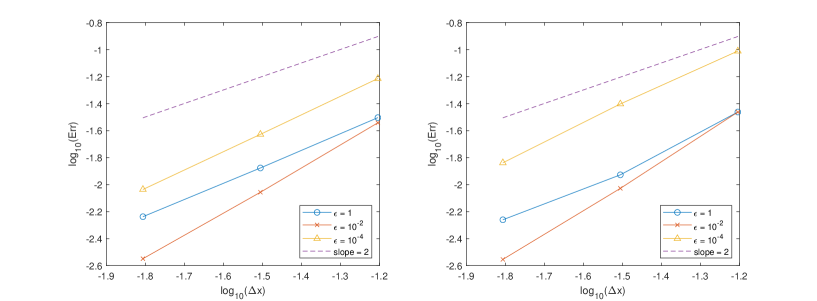
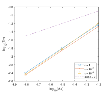
The convergence order in $l^{1}$ norm for the particle distribution $f_{i}(i=1,2)$ and in $l^{2}$ norm for the fluid velocity $\mathbf{u}$ is reported in Figures 1-2. This shows that the scheme is second order in space (hence in time) uniformly in $\varepsilon$ for both the particle distributions $f_{i}$ and the fluid velocity $\mathbf{u}$ as expected.

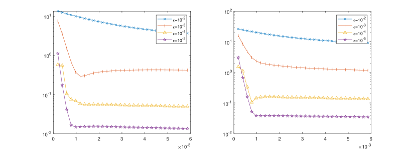
4.2 AP property

Now we check the AP property. We take the volcano like initial data:

		$\displaystyle n_{1}(0,\mathbf{x})=n_{2}(0,\mathbf{x})$		(4.2)
		$\displaystyle\quad\quad\quad\ =\left(0.5+100\left((x_{1}-0.5)^{2}+(x_{2}-0.5)^{2}\right)\right)\exp\left(-40(x_{1}-0.5)^{2}-40(x_{2}-0.5)^{2}\right),$
		$\displaystyle\mathbf{u}_{p,1}(0,\mathbf{x})=\mathbf{u}_{p,2}(0,\mathbf{x})=\left(\begin{array}[]{c}-\sin(2\pi(x_{2}-0.5))\\ \sin(2\pi(x_{1}-0.5))\end{array}\right)\exp\left(-20(x_{1}-0.5)^{2}-20(x_{2}-0.5)^{2}\right),$
		$\displaystyle\mathbf{u}(0,\mathbf{x})=0.$

The time evolution of $\ell^{1}$ distances $\left\|f_{i}-n_{i}M_{u,i}\right\|_{1}$ where $M_{u,i}$ is a Maxwellian centered at the fluid velocity $u$ is shown in Fig. 3. The result gives a direct evidence of the AP property we proposed.

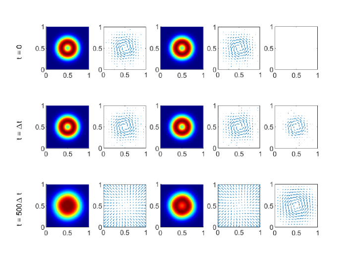
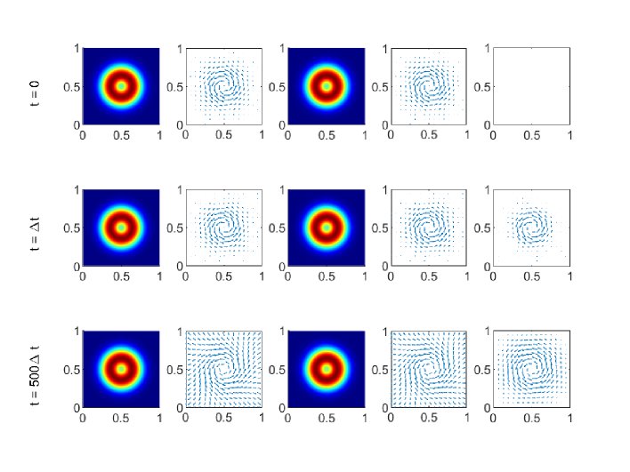
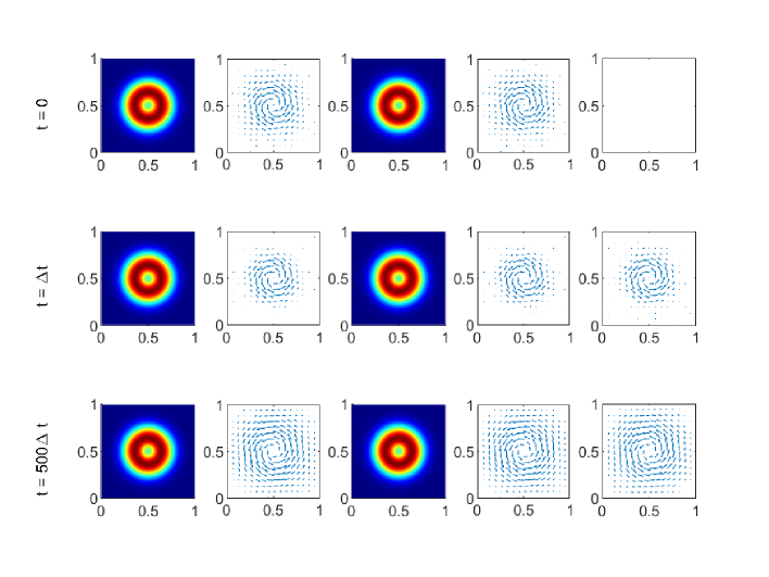
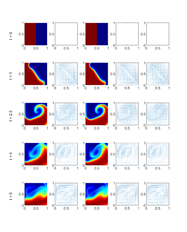
For the initial data (4.2), $\mathbf{u}_{p,i}\neq\mathbf{u}$ $(i=1,2)$ and thus the equilibrium is not assumed. Figure 4 gives the time evolution of the system (4.2) with $\varepsilon=1$ at $t^{0}$ (the initial time), $t^{1}$ (after one time step) and $t^{500}$ (the end time). The left two columns show the particle density $n_{1}$ and streamlines of particle velocity $\mathbf{u}_{p,1}$ of the first particle $(i=1)$ . The third and fourth columns show the particle density $n_{2}$ and streamlines of particle velocity $\mathbf{u}_{p,2}$ of the second particle $(i=2)$ . The right column give the fluid velocity $\mathbf{u}$ . In Figure 4, the particles expand to the whole square domain and are not significantly affected by the circulating fluid. The streamlines of particles and fluid are quite different because the drag force bewteen the fluid phase and particle phases is not significant. The behavior turns out to be significantly different as $\varepsilon$ decreases.

Figures 5 gives the time evolution of this system (4.2) with $\varepsilon=10^{-3}$ . In the case with smaller $\varepsilon$ , the drag force between different phases is much stronger that the particles also circulate in the square domain. Besides, the expansion in particle density is decelerated by the fluid.

Figures 6 gives the time evolution of this system (4.2) with $\varepsilon=10^{-5}$ . In this case, the particles stop expanding immediately due to the strong drag force. The particles keep the volcano shape well in this period of time.

4.3 Some applications

In this section we apply our schemes to several different problems. In the following simulation we will take $Re=1000$ . Larger Reynolds number, which requires smaller mesh size $\Delta x$ for the sake of accuracy, is beyond the scope of this work. In Section 4.3.1 the external force (the gravity) is considered and in Section 4.3.2 we perform a simulation with $\varepsilon$ varying in space.

4.3.1 Simulationof gravity driven flow

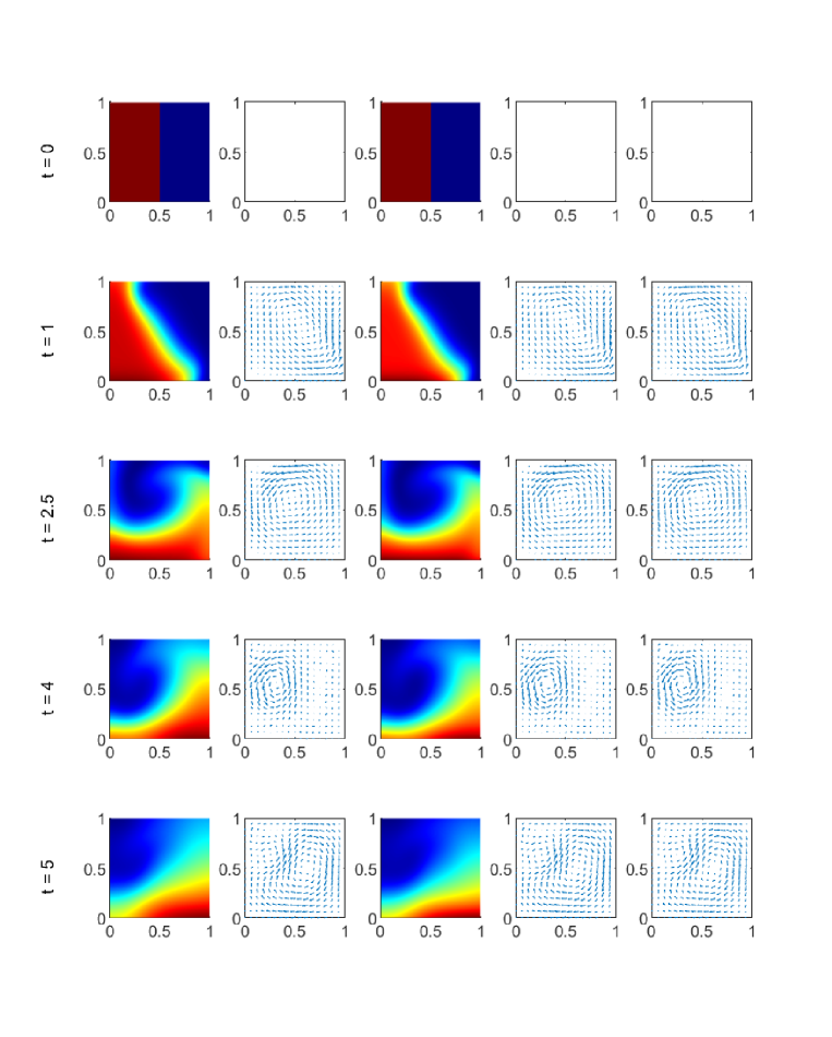
Now we consider the dam like initial data,

		$\displaystyle n_{1}(0,\mathbf{x})=n_{2}(0,\mathbf{x})=10^{-10}+1_{0\leqslant x\leqslant 0.5},$		(4.3)
		$\displaystyle\mathbf{u}_{p,1}(0,\mathbf{x})=\mathbf{u}_{p,2}(0,\mathbf{x})=0,$
		$\displaystyle\mathbf{u}(0,\mathbf{x})=0.$

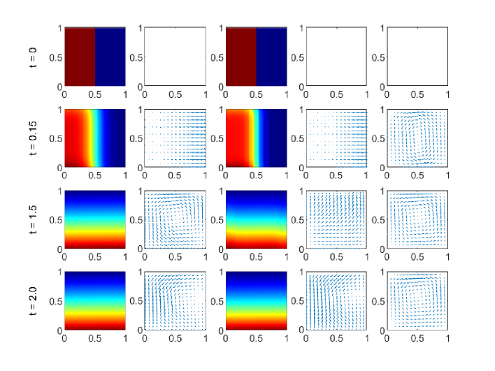
In this case the movement of particles and fluid are initiated by the gravity. As the simulation starts, the particles fall down and cause the circulation of fluid.

Fig. 7 shows the time evolution of the density and streamlines of the velocity for the small particle (left two columns) with $\varepsilon=1$ , as well as the time evolution of the density and streamlines of the velocity for the large particle (third and fourth column) and fluid velocity (right column). In this case the drag force between particles and fluid is not significant. The particles just fall down and cover the whole bottom. Clearly, the streamlines of particles is quite different from that of the fluid. The first particle with smaller size evolves faster than the second particle with larger size. In other words, the light species gets close to the Maxwellian faster than the heavy one, which is consistent with the observation verified in [26] for multi-species Boltzmann equations.

Fig. 8 shows the time evolution of particle density with $\varepsilon=10^{-2}$ . Now the drag force between particles and fluid is stronger. The streamlines of particles and the fluid are similar all the time. As time evolves, the particles fall down and drive the fluid to circulate counter-clockwisely. Then the particles follow this circulation. Finally the particles settle at the bottom uniformly due to the loss of energy.

Fig. 9 shows the time evolution of particle density with $\varepsilon=10^{-3}$ . In this case the drag force between particles and fluid is so strong that the streamlines of the particles and fluid are quite similar to each other.

4.3.2 Simulation of injecting problem

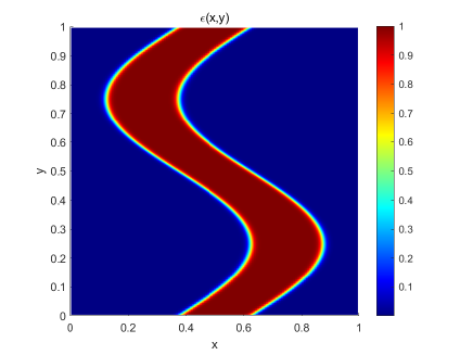
One of the advantages of AP schemes is that they can capture the solution behaviors automatically as $\varepsilon$ varies in space. Finally, let us consider a mixing regime problem, with an $\mathbf{x}$ -dependent $\varepsilon(\mathbf{x})$

\varepsilon(x,y)=\varepsilon_{0}+\frac{1}{2}\left(\tanh\left(10-80\left(x-\frac{1}{2}-\frac{1}{4}\sin(2\pi y)\right)\right)+\tanh\left(10+80\left(x-\frac{1}{2}-\frac{1}{4}\sin(2\pi y)\right)\right)\right).

(4.4)

Here $\varepsilon_{0}\ll 1$ is a constant. $\varepsilon(\mathbf{x})$ varies from $\varepsilon_{0}$ to $O(1)$ smoothly, as shown in Figure 10 with $\varepsilon_{0}=10^{-3}$ .

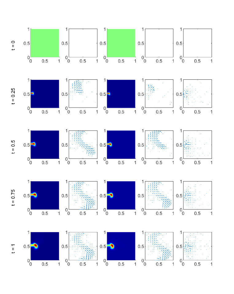
Consider the situation when the particles are injected into the square domain. More specifically, the initial conditions are given as follows.

n_{1}(0,\mathbf{x})=n_{2}(0,\mathbf{x})=10^{-10},\quad\mathbf{u}_{p,1}(0,\mathbf{x})=\mathbf{u}_{p,2}(0,\mathbf{x})=\mathbf{u}(0,\mathbf{x})=0.

(4.5)

The injecting particle flow is described by the boundary condition on $f_{i}(i=1,2)$ ,

		$\displaystyle f_{1}(t,\mathbf{x},\mathbf{v})=1_{2\leqslant v_{1}\leqslant 3},\quad\text{ if }\mathbf{x}\in\Gamma=\{(0,y)\mid 0.475\leqslant y\leqslant 0.575\},$		(4.6)
		$\displaystyle f_{2}(t,\mathbf{x},\mathbf{v})=1_{2\leqslant v_{1}\leqslant 3},\quad\text{ if }\mathbf{x}\in\Gamma=\{(0,y)\mid 0.45\leqslant y\leqslant 0.55\},$		(4.6)

where $v_{1}$ is the first component of $\mathbf{v}$ . The entrance of flow $\Gamma$ locates at the center of the left boundary.

Figure 11 shows several snapshots of the time evolution of the particle density $n_{1},n_{2}$ , streamlines of prticle velocity $u_{p,1},u_{p,2}$ and the fluid velocity $u$ . The behaviors of both phases are clearly influenced by the spatially variable $\varepsilon(\mathbf{x})$ . The first particle with smaller size evolves a little faster than the second particle with larger size. The difference of the velocities of two phases $\left|\mathbf{u}_{p}-\mathbf{u}\right|$ shows an S-shape profile which is consistent to $\varepsilon(\mathbf{x})$ in Figure 10. This suggests that the fluid limit of this two-phase system is achieved automatically in the strong interaction regime where $\varepsilon\ll 1$ . While in the weak interaction regimes where $\varepsilon=O(1)$ the two phases behave quite differently.

5 Conclusion

We have introduced a new numerical scheme for simulating a system coupling the incompressible Navier–Stokes equation to multi-component Vlasov–Fokker–Planck equations with distinct particle sizes. In particular, the scheme is Asymptotic Preserving, which drives the system towards a set of hydrodynamic equations in the regime of $\varepsilon\ll 1$ . The method is based on the implicit treatment of the potentially stiff terms and relies on the possibility of updating the macroscopic unknowns by solving simple linear systems. It is interesting that in the multi-phase kinetic-fluid system, the smaller particle with light mass evolves a little faster than the bigger particle with heavy mass, and thus the smaller particle may get close to the equilibrium faster than the bigger one. The scheme can easily incorporate relevant generalizations of the basic model like considering variable fluid density or temperature-dependent viscosities. Furthermore, the scheme can be used for the kinetic-fluid system with multi-size particles with uncertainties.

Acknowledgement

S. Jin was partially supported by National Key R&D Program of China (no. 2020YFA0712000) and National Natural Science Foundation of China (no. 20Z103020029). Y. Lin was partially supported by National Natural Science Foundation of China (no. 12201404) and Postdoctoral Research Foundation of China (no. 2021M702142 and no. 2021TQ0203). Y. Lin thanks Dr. Ruiwen Shu for his help during the preparation of the paper.

Appendix

Scaling issues. Let us detail precisely the scaling issues and the physical meaning of the system we are interested in. To this end, let us go back to the equations written with dimensional quantities.

We adopt a multi-component Vlasov-Fokker-Planck-incompressible Navier-Stokes system for a discrete modeling of $N$ -size variable for particles. Let $i\in\{1,2,\ldots N\}$ . We refer to ” a particle size $i$ ” as an assembly of $i$ monomers. As usual, the fluid is described by its density $n(t,x)$ and velocity $u(t,x)$ , which obey the mass conservation and momentum balance relations. Denoting by $a>0$ the radius of a monomer and $\rho_{P}$ its mass density, the radius and mass of an $i$ -mer are defined by

r_{i}=ai^{1/3},\quad m_{i}=\frac{4}{3}\pi a^{3}i\rho_{P}=m_{1}i\text{~{}~{}with~{}}m_{1}=\frac{4}{3}\pi a^{3}\rho_{P}

respectively. The particles are described by the quantity $f_{i}(t,x,v)$ such that $f_{i}(t,x,v)\mathrm{~{}d}v\mathrm{~{}d}x$ is the probability of finding particles with size $i$ in the domain of the phase space centered at $(x,v)$ with volume $\mathrm{~{}d}v\mathrm{~{}d}x$ . Particles are subject to the Brownian motion, which induces a diffusion term whose coefficient is given by Einstein formula [13]

\frac{9\mu}{2\rho_{P}r_{i}^{2}}\frac{k\theta}{m_{i}}

where $k$ is the Boltzmann constant, $\theta>0$ is temperature of the fluid and $\mu$ is dynamic viscosity of the fluid. The drag force exerted by the fluid on the particles is given by the Stokes law, which is proportional to the relative velocity

6\pi\mu r_{i}(v-u)=6\pi\mu ai^{1/3}(v-u).

The Sokes settling time is defined by

\tau_{i}=\frac{m_{i}}{6\pi\mu r_{i}}=\dfrac{2\rho_{P}r_{i}^{2}}{9\mu}=i^{2/3}\tau_{1}\quad\text{ with }\tau_{1}=\dfrac{2\rho_{P}a^{2}}{9\mu},

which is typical of the effect of the drag force on the $i$ -particle. Denoting by $\rho_{F}>0$ a typical mass density for the fluid and introducing the $i$ th Fokker-Planck (FP) operator $\mathcal{L}_{u}f_{i}$ by

\mathcal{L}_{u}f_{i}=\nabla_{v}\cdot\left((v-u)f_{i}+\dfrac{k\theta}{m_{i}}\nabla_{v}f_{i}\right),

the particles-fluid mixture with distinct particle size is then described by the followign system of PDEs:

\left\{\begin{array}[]{l}\partial_{t}f_{i}+v\cdot\nabla_{x}f_{i}-\nabla_{x}\Phi\cdot\nabla_{v}f_{i}=\dfrac{9\mu}{2\rho_{P}r_{i}^{2}}\mathcal{L}_{u}f_{i},\\ \rho_{F}\partial_{t}(u)+\rho_{F}\operatorname{Div}_{x}(u\otimes u)+\rho_{F}\alpha\nabla_{x}\Phi+\nabla_{x}p-\mu\Delta_{x}u=\displaystyle 6\pi\mu\sum_{i=1}^{N}\int_{\mathbb{R}^{3}}(v-u)f_{i}r_{i}\mathrm{~{}d}v,\\ \nabla_{x}\cdot u=0.\end{array}\right.

(5.1)

Following [9, 20], we are going to write system (5.1) in dimensionless form. To this end, we introduce time and length scales, denoted by $T$ and $L$ , respectively, which define the velocity unit $U=L/T$ . Set the thermal velocity $V=\sqrt{\frac{k\bar{\theta}}{m_{1}}}$ with $m_{1}=\frac{4}{3}\pi a^{3}\rho_{P}$ and $\bar{\theta}>0$ a reference temperature. Set $\mathcal{P}$ a suitable pressure unit. The dimensionless variables and unknowns can be defined as follows:

1.

$t^{\prime}=t/T,x^{\prime}=x/L,v^{\prime}=v/V$ ,
2.

$n^{\prime}\left(t^{\prime},x^{\prime}\right)=n\left(Tt^{\prime},Lx^{\prime}\right),u^{\prime}\left(t^{\prime},x^{\prime}\right)=u\left(Tt^{\prime},Lx^{\prime}\right)/U$ ,
3.

$p^{\prime}\left(t^{\prime},x^{\prime}\right)=p\left(Tt^{\prime},Lx^{\prime}\right)/\mathcal{P},f_{i}^{\prime}\left(t^{\prime},x^{\prime},v^{\prime}\right)=\frac{4}{3}\pi a^{3}V^{3}f_{i}\left(Tt^{\prime},Lx^{\prime},Vv^{\prime}\right)$ .

Since $\mathrm{~{}d}v^{\prime}=\mathrm{d}v/V^{3}$ , for any given function $\varphi$ , one has

\int_{\mathbb{R}^{3}}\varphi(v)f_{i}(t,x,v)\mathrm{d}v=\frac{1}{\frac{4}{3}\pi a^{3}}\int_{\mathbb{R}^{3}}\varphi\left(Vv^{\prime}\right)f_{i}^{\prime}\left(t^{\prime},x^{\prime},v^{\prime}\right)\mathrm{d}v^{\prime}.

If the temperature is not assumed constant, similarly set $\theta^{\prime}\left(t^{\prime},x^{\prime}\right)=\theta\left(Tt^{\prime},Lx^{\prime}\right)/\bar{\theta}$ . For the external potential, set $\Phi^{\prime}\left(x^{\prime}\right)=\Phi\left(Lx^{\prime}\right)\frac{\tau_{1}}{\vartheta_{s}L}$ , where $\vartheta_{s}$ has the dimension of velocity (for gravity-driven flows, it is the Stokes settling velocity). One arrives at

\displaystyle\frac{1}{T}\partial_{t^{\prime}}\left(f_{i}^{\prime}\right)

\displaystyle+\frac{V}{L}v^{\prime}\cdot\nabla_{x^{\prime}}\left(f_{i}^{\prime}\right)-\frac{\vartheta_{s}}{\tau_{1}V}\nabla_{x^{\prime}}\Phi^{\prime}\cdot\nabla_{v^{\prime}}\left(f_{i}\right)=\frac{1}{\tau_{i}}\nabla_{v^{\prime}}\cdot\left(\left(v^{\prime}-\frac{U}{V}u^{\prime}\right)f_{i}^{\prime}+\frac{k\bar{\theta}}{m_{i}V^{2}}\theta^{\prime}\nabla_{v^{\prime}}f_{i}^{\prime}\right).

Therefore, we realize that the system is driven by the following set of dimensionless paratmeters:

\beta=\frac{T}{L}V=\frac{V}{U},\quad\frac{1}{\varepsilon}=\frac{T}{\tau_{1}},\quad\eta=\frac{\vartheta_{s}T}{V\tau_{1}},\quad\chi=\frac{\mathcal{P}T}{\rho_{F}LU}=\frac{\mathcal{P}}{\rho_{F}U^{2}},

together with the density ratio $\rho_{P}/\rho_{F}$ . Finally, by dropping the prime marks, one obtains the dimensionles form of system (5.1):

\displaystyle\left\{\begin{array}[]{l}\partial_{t}f_{i}+\beta v\cdot\nabla_{x}f_{i}-\eta\nabla_{x}\Phi\cdot\nabla_{v}f_{i}=\dfrac{1}{\varepsilon}\dfrac{1}{i^{2/3}}\nabla_{v}\cdot\left(\left(v-\dfrac{1}{\beta}u\right)f_{i}+\dfrac{\bar{\theta}}{i}\nabla_{v}f_{i}\right),\\ \partial_{t}(u)+\operatorname{Div}_{x}(u\otimes u)+\alpha\beta\eta\nabla_{x}\Phi+\chi\nabla_{x}p=\dfrac{\rho_{P}}{\varepsilon\rho_{F}}\displaystyle\sum_{i=1}^{N}\displaystyle\int_{\mathbb{R}^{3}}(\beta v-u)f_{i}i^{1/3}\mathrm{~{}d}v+\mu\Delta_{x}u,\\ \nabla_{x}\cdot u=0.\end{array}\right.

(5.2)

Here $\mu$ stands for the rescaled and dimensionless version of the fluid viscosity.

References

Andrews and O’Rourke [1996] Andrews, M.J., O’Rourke, P.J., 1996. The multiphase particle-in-cell (mp-pic) method for dense particulate flows. International Journal of Multiphase Flow 22, 379–402.
Aregba-Driollet and Milisik [2004] Aregba-Driollet, D., Milisik, V., 2004. Kinetic approximation of a boundary value problem for conservation laws. Numerische Mathematik 97, 595–633.
Baranger et al. [2005] Baranger, C., Boudin, L., Jabin, P.E., Mancini, S., 2005. A modeling of biospray for the upper airways, in cemracs 2004—mathematics and applications to biology and medicine. ESAIM: Proc. 14, EDP Sci., Les Ulis, France , 41–47.
Baranger and Desvillettes [2006] Baranger, C., Desvillettes, L., 2006. Coupling euler and vlasov equations in the context of sprays: the local-in-time, classical solutions. Journal of Hyperbolic Differential Equations 3, 1–26.
Boudin et al. [2009a] Boudin, L., Boutin, B., Fornet, B., Goudon, T., Lafitte, P., Lagoutière, F., Merlet, B., 2009a. Fluid-particles flows: A thin spray model with energy exchanges, in: ESAIM: Proceedings, EDP Sciences. pp. 195–210.
Boudin et al. [2009b] Boudin, L., Desvillettes, L., Grandmont, C., Moussa, A., 2009b. Global existence of solutions for the coupled vlasov and navier-stokes equations. Differential and Integral Equations 22, 1247–1271.
Carrillo et al. [2011] Carrillo, J.A., Duan, R., Moussa, A., 2011. Global classical solutions close to equilibrium to the vlasov-fokker-planck-euler system. Kinetic & Related Models 4, 227–258.
Carrillo et al. [2008] Carrillo, J.A., Goudon, T., Lafitte, P., 2008. Simulation of fluid and particles flows: Asymptotic preserving schemes for bubbling and flowing regimes. Journal of Computational Physics 227, 7929–7951.
Carrilo and Goudon [2006] Carrilo, J., Goudon, T., 2006. Stability and asymptotic analysis of a fluid-particles interaction model. Communications in Partial Differential Equations 31, 1349–1379.
Chorin [1967] Chorin, A.J., 1967. The numerical solution of the navier-stokes equations for an incompressible fluid. Bulletin of the American Mathematical Society 73, 928–931.
Chorin [1969] Chorin, A.J., 1969. On the convergence of discrete approximations to the navier-stokes equations. Mathematics of computation 23, 341–353.
Cober and Isaac [2006] Cober, S., Isaac, G., 2006. Estimating Maximum Aircraft Icing Environments Using a Large Database of In-Situ Observations. 44th AIAA Aerospace Sciences Meeting and Exhibit, AIAA 2006-266.
Einstein [1906] Einstein, A., 1906. Eine neue bestimmung der moleküldimensionen. Ann. Physik 19, 289–306.
Friedlander [1977] Friedlander, S.K., 1977. Smoke, Dust and Haze: Fundamentals of Aerosol Behavior. Wiley-Interscience, New York.
Goudon et al. [2010] Goudon, T., He, L., Moussa, A., Zhang, P., 2010. The navier–stokes–vlasov–fokker–planck system near equilibrium. SIAM Journal on Mathematical Analysis 42, 2177–2202.
Goudon et al. [2004a] Goudon, T., Jabin, P.E., Vasseur, A., 2004a. Hydrodynamic limit for the Vlasov-Navier-Stokes equations. I. Light particles regime. Indiana University Mathematics Journal 53, 1517–1536.
Goudon et al. [2004b] Goudon, T., Jabin, P.E., Vasseur, A., 2004b. Hydrodynamic limit for the Vlasov-Navier-Stokes equations. II. Fine particles regime. Indiana University Mathematics Journal 53, 1495–1515.
Goudon et al. [2013a] Goudon, T., Jin, S., Liu, J.G., Yan, B., 2013a. Asymptotic-preserving schemes for kinetic-fluid modeling of disperse two-phase flows. Journal of Computational Physics 246, 145–164.
Goudon et al. [2012] Goudon, T., Jin, S., Yan, B., 2012. Simulation of fluid-particles flows: heavy particles, flowing regime and asymptotic-preserving schemes. Communications in Mathematical Sciences 10, 355–385.
Goudon et al. [2013b] Goudon, T., Sy, M., Tine, L.M., 2013b. A fluid-kinetic model for particulate flows with coagulation and breakup: stationary solutions, stability, and hydrodynamic regimes. SIAM Journal on Applied Mathematics 73, 401–421.
Hamdache [1998] Hamdache, K., 1998. Global existence and large time behaviour of solutions for the vlasov-stokes equations. Japan Journal of Industrial and Applied Mathematics 51, 51–74.
Hauf and Schröder [2006] Hauf, T., Schröder, F., 2006. Aircraft icing research flights in embedded convection. Meteorology and Atmospheric Physics 91, 247–265.
Jin [1999] Jin, S., 1999. Efcient asymptotic-preserving (AP) schemes for some multiscale kinetic equations. SIAM Journal on Scientific Computing 21, 441–454.
Jin [2010] Jin, S., 2010. Asymptotic preserving (ap) schemes for multiscale kinetic and hyperbolic equations: a review. Lecture notes for summer school on methods and models of kinetic theory (M&MKT), Porto Ercole (Grosseto, Italy) , 177–216.
Jin [2022] Jin, S., 2022. Asymptotic-preserving schemes for multiscale physical problems. Acta Numerica 31, 415–489.
Jin and Li [2013] Jin, S., Li, Q., 2013. A bgk-penalization-based asymptotic-preserving scheme for the multispecies boltzmann equation. Numerical Methods for Partial Differential Equations 29, 1056–1080.
Jin and Lin [2022] Jin, S., Lin, Y., 2022. Energy estimates and hypocoercivity analysis for a multi-phase navier-stokes-vlasov-fokker-planck system with uncertainty arXiv:2204.10573.
Jin and Yan [2011] Jin, S., Yan, B., 2011. A class of asymptotic-preserving schemes for the fokker–planck–landau equation. Journal of Computational Physics 230, 6420–6437.
Liu et al. [2011] Liu, H., Wang, Z., Fox, R.O., 2011. A level set approach for dilute non-collisional fluid-particle flows. Journal of Computational Physics 230, 920–936.
Mellet and Vasseur [2007] Mellet, A., Vasseur, A., 2007. Global weak solutions for a vlasov–fokker–planck/navier–stokes system of equations. Mathematical Models and Methods in Applied Sciences 17, 1039–1063.
Mellet and Vasseur [2008] Mellet, A., Vasseur, A., 2008. Asymptotic analysis for a vlasov-fokker-planck/compressible navier-stokes system of equations. Communications in Mathematical Physics 281, 573–596.
Patankar and Joseph [2001a] Patankar, N., Joseph, D., 2001a. Lagrangian numerical simulation of particulate flows. International Journal of Multiphase Flow 27, 1685–1706.
Patankar and Joseph [2001b] Patankar, N., Joseph, D., 2001b. Modeling and numerical simulation of particulate flows by the eulerian–lagrangian approach. International Journal of Multiphase Flow 27, 1659–1684.
Potapczuk and Tsao [2019] Potapczuk, M., Tsao, J., 2019. The Influence of SLD Drop Size Distributions on Ice Accretion in the NASA Icing Research Tunnel. SAE Technical Paper.
Prosperetti and Tryggvason [2007] Prosperetti, A., Tryggvason, G., 2007. Computational Methods for Multiphase Flows. Cambridge University Press, Cambridge, UK.
Williams [1985] Williams, F.A., 1985. Combustion Theory, 2nd ed. Benjamin Cummings, Menlo Park, CA.
Yu [2013] Yu, C., 2013. Global weak solutions to the incompressible navier–stokes–vlasov equations. Journal de Mathématiques Pures et Appliquées 100, 275–293.

		$\displaystyle\frac{1}{2\Delta t}\left(3J_{i}^{*}-4J_{i}^{k}+J_{i}^{k-1}\right)$		(3.9)
		$\displaystyle\quad=-\int v\otimes v\nabla_{x}(2f_{i}^{k}-f_{i}^{k-1})\mathrm{d}v-(2n_{i}^{k}-n_{i}^{k-1})\nabla_{x}\Phi-\frac{1-\alpha}{i^{2/3}\varepsilon}\left(J_{i}^{}-in_{i}^{k+1}u^{}\right)$
		$\displaystyle\frac{1}{2\Delta t}\left(3u^{}-4u^{k}+u^{k-1}\right)-\dfrac{1}{Re}\Delta_{x}u^{}+\nabla_{x}p^{k}$
		$\displaystyle\quad=-\nabla_{x}\cdot(2(u^{k}\otimes u^{k})-(u^{k-1}\otimes u^{k-1}))+\sum_{i=1}^{N}\frac{(1-\alpha)\rho_{P}}{i^{2/3}\varepsilon\rho_{F}}\left(J_{i}^{}-in_{i}^{k+1}u^{}\right)$