This paper was converted on www.awesomepapers.org from LaTeX by an anonymous user.
Want to know more? Visit the Converter page.

Asymptotic properties of generalized eigenfunctions for multi-dimensional quantum walks

Takashi Komatsu Department of Bioengineering, School of Engineering,The University of Tokyo, Bunkyo-ku, Tokyo, 113-8656, Japan komatsu@coi.t.u-tokyo.ac.jp Norio Konno Department of Applied Mathematics, Yokohama National University, Hodogaya, Yokohama, Kanagawa, 240-8501, Japan konno-norio-bt@ynu.ac.jp Hisashi Morioka Graduate School of Science and Engineering, Ehime University, Bunkyo-cho 3, Matsuyama, Ehime, 790-8577, Japan morioka@cs.ehime-u.ac.jp  and  Etsuo Segawa Graduate School of Environment and Information Sciences, Yokohama National University, Hodogaya, Yokohama, Kanagawa, 240-8501, Japan segawa-etsuo-tb@ynu.ac.jp
Abstract.

We construct a distorted Fourier transformation associated with the multi-dimensional quantum walk. In order to avoid the complication of notations, almost all of our arguments are restricted to two dimensional quantum walks (2DQWs) without loss of generality. The distorted Fourier transformation characterizes generalized eigenfunctions of the time evolution operator of the QW. The 2DQW which will be considered in this paper has an anisotropy due to the definition of the shift operator for the free QW. Then we define an anisotropic Banach space as a modified Agmon-Hörmander’s \mathcal{B}^{*} space and we derive the asymptotic behavior at infinity of generalized eigenfunctions in these spaces. The scattering matrix appears in the asymptotic expansion of generalized eigenfunctions.

Key words and phrases:
quantum walk, scattering matrix, Green function
2010 Mathematics Subject Classification:
Primary 81U20, Secondary 47A40
H. Morioka is supported by the JSPS Grant-in-aid for young scientists No. 20K14327. E. Segawa is supported by the JSPS Grant-in-Aid for Scientific Research (C) No. 19K03616 and Research Origin for Dressed Photon.

1. Introduction

1.1. Scattering theory for multi-dimensional quantum walk

In this paper, we consider the time-independent scattering theory for the position-dependent dd-dimensional quantum walk (ddDQW or simply QW for short) as a finite rank perturbation of the ddD free QW which is defined as follows. The states of quantum walker on 𝐙d={x=(x1,,xd);x1,,xd𝐙}{\bf Z}^{d}=\{x=(x_{1},\ldots,x_{d})\ ;\ x_{1},\ldots,x_{d}\in{\bf Z}\} are represented by ψ={ψ(x)}x𝐙d\psi=\{\psi(x)\}_{x\in{\bf Z}^{d}} which are 𝐂2d{\bf C}^{2d}-valued sequences. Letting 𝖳*^{\mathsf{T}} be the transpose operator for matrices or vectors, we denote by the column vector

ψ(x)=[ψ1+(x),ψ1(x),,ψd+(x),ψd(x)]𝖳,x𝐙d,\psi(x)=[\psi^{+}_{1}(x),\psi^{-}_{1}(x),\ldots,\psi^{+}_{d}(x),\psi^{-}_{d}(x)]^{\mathsf{T}},\quad x\in{\bf Z}^{d},

for 𝐂{\bf C}-valued sequences ψj±\psi^{\pm}_{j} for j=1,,dj=1,\ldots,d on 𝐙d{\bf Z}^{d}. Each component ψj±(x)\psi_{j}^{\pm}(x) corresponds the “probability amplitude” at x𝐙dx\in{\bf Z}^{d} of the chirality (j,±)(j,\pm). The ddD free QW is defined by the operator U0=SU_{0}=S where SS is the shift operator :

(Sψ)(x)=[ψ1+(x+e1),ψ1(xe1),,ψd+(x+ed),ψd(xed)]𝖳,(S\psi)(x)=[\psi_{1}^{+}(x+e_{1}),\psi_{1}^{-}(x-e_{1}),\ldots,\psi_{d}^{+}(x+e_{d}),\psi_{d}^{-}(x-e_{d})]^{\mathsf{T}},

where e1,,ede_{1},\ldots,e_{d} are the standard basis on 𝐙d{\bf Z}^{d}. The position-dependent QW is defined by the operator U=SCU=SC where CC is the operator of multiplication by a matrix C(x)=(ck,l(x))k,l=12dU(2d)C(x)=(c_{k,l}(x))_{k,l=1}^{2d}\in\mathrm{U}(2d) for every x𝐙dx\in{\bf Z}^{d}. Throughout of this paper, we assume that the following statements hold.

  • There exists a positive integer n0n_{0} such that C(x)C(x) is the 2d×2d2d\times 2d identity matrix I2dI_{2d} for x𝐙dDx\in{\bf Z}^{d}\setminus D where D={x𝐙d;|x1|n0,,|xd|n0}D=\{x\in{\bf Z}^{d}\ ;\ |x_{1}|\leq n_{0},\ldots,\ |x_{d}|\leq n_{0}\}.

  • For every xDx\in D,

    det(c2k1,2l1(x))k,l=1d,det(c2k,2l(x))k,l=1d,\mathrm{det}(c_{2k-1,2l-1}(x))_{k,l=1}^{d},\quad\mathrm{det}(c_{2k,2l}(x))_{k,l=1}^{d},

    do not vanish.

These assumptions will be used in order to prove a unique continuation property for generalized eigenfunctions of UU in Lemma 3.7 and Corollary 3.8. The unique continuation property guarantees a radiation condition for non-homogeneous equations and the absence of eigenvalues of UU. See Corollaries 3.11 and 3.12.

In the following, almost all of our arguments are restricted to the case d=2d=2 in order to avoid the complication of notations. Our results can be generalized easily for higher dimensional cases. For the case d=2d=2, we use more explicit notations. Components of 𝐂4{\bf C}^{4}-valued sequences ψ\psi are written as

ψ(x)=[ψ(x),ψ(x),ψ(x),ψ(x)]𝖳,x𝐙2.\psi(x)=[\psi_{\leftarrow}(x),\psi_{\rightarrow}(x),\psi_{\downarrow}(x),\psi_{\uparrow}(x)]^{\mathsf{T}},\quad x\in{\bf Z}^{2}.

The chirality of ψ\psi is represented by p{,,,}p\in\{\leftarrow,\rightarrow,\downarrow,\uparrow\}. Typical examples of C(x)C(x) for every xDx\in D such that the second assumption holds are

12[1111111111111111],[1/21/61/121/21/21/61/121/202/61/121/2003/121/2].\frac{1}{2}\left[\begin{array}[]{cccc}1&1&1&1\\ 1&-1&1&-1\\ 1&1&-1&-1\\ 1&-1&-1&1\end{array}\right],\quad\left[\begin{array}[]{cccc}1/\sqrt{2}&1/\sqrt{6}&1/\sqrt{12}&1/2\\ -1/\sqrt{2}&1/\sqrt{6}&1/\sqrt{12}&1/2\\ 0&-2/\sqrt{6}&1/\sqrt{12}&1/2\\ 0&0&3/\sqrt{12}&-1/2\end{array}\right].

On the other hand, the 2D Grover coin and the 2D Fourier coin

12[1111111111111111],12[11111i1i11111i1i],\frac{1}{2}\left[\begin{array}[]{cccc}-1&1&1&1\\ 1&-1&1&1\\ 1&1&-1&1\\ 1&1&1&-1\end{array}\right],\quad\frac{1}{2}\left[\begin{array}[]{cccc}1&1&1&1\\ 1&i&-1&-i\\ 1&-1&1&-1\\ 1&-i&-1&i\end{array}\right],

do not satisfy the second assumption.

Obviously, operators U0U_{0} and UU are unitary on the Hilbert space 2:=2(𝐙2;𝐂4)\ell^{2}:=\ell^{2}({\bf Z}^{2};{\bf C}^{4}) equipped with the standard inner product

(f,g)2=p{,,,}x𝐙2fp(x)gp(x)¯.(f,g)_{\ell^{2}}=\sum_{p\in\{\leftarrow,\rightarrow,\downarrow,\uparrow\}}\sum_{x\in{\bf Z}^{2}}f_{p}(x)\overline{g_{p}(x)}.

The discrete time evolutions of these QWs are given by

Ψ(t,)=Utψ,Ψ(0)(t,)=U0tψ,t𝐙,\Psi(t,\cdot)=U^{t}\psi,\quad\Psi^{(0)}(t,\cdot)=U_{0}^{t}\psi,\quad t\in{\bf Z},

for an initial state ψ\psi. If ψ2\psi\in\ell^{2}, these time evolutions preserve the 2\ell^{2}-norm of ψ\psi i.e. Ψ(t,)2=Ψ(0)(t,)2=ψ2\|\Psi(t,\cdot)\|_{\ell^{2}}=\|\Psi^{(0)}(t,\cdot)\|_{\ell^{2}}=\|\psi\|_{\ell^{2}} for any t𝐙t\in{\bf Z}.

In view of the quantum scattering theory, the scattering matrix (S-matrix) is an important object. There are several equivalent definitions of the S-matrix. In the time-dependent scattering theory, we can prove that the wave operators

W±=s-limt±UtU0tin2W_{\pm}={\mathop{{\rm s\text{-}lim}}_{t\to\pm\infty}}\,U^{-t}U_{0}^{t}\quad\text{in}\quad\ell^{2}

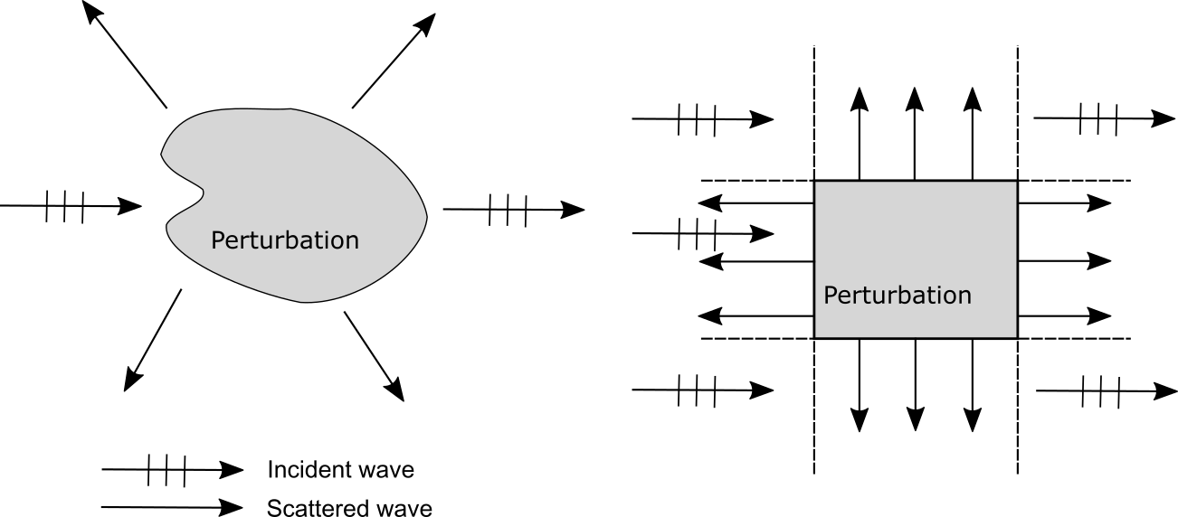
exist and asymptotically complete under our assumption by the similar way of Suzuki [21]. Namely, we have the following fact on the long time behavior of QWs. See also Figure 1.

Proposition 1.1.

The ranges of the wave operators coincide with ac(U)\mathcal{H}_{ac}(U), the absolutely continuous subspace for UU. In particular, for any ϕac(U)\phi\in\mathcal{H}_{ac}(U), there exist ψ±2\psi_{\pm}\in\ell^{2} such that UtϕU0tψ±20\|U^{t}\phi-U^{t}_{0}\psi_{\pm}\|_{\ell^{2}}\to 0 as t±t\to\pm\infty. The wave operators are unitary on 2\ell^{2} and we have W±=W±1W_{\pm}^{*}=W_{\pm}^{-1}.

Refer to caption
Figure 1. For an initial state ϕac(U)\phi\in\mathcal{H}_{ac}(U), there exist ψ±2\psi_{\pm}\in\ell^{2} such that UtϕU0tψ±U^{t}\phi\sim U_{0}^{t}\psi_{\pm} as t±t\to\pm\infty. The wave operators represent these asymptotic behaviors. Roughly speaking, the scattering in view of the dynamics of UtϕU^{t}\phi is a transition from a free QW U0tψU_{0}^{t}\psi_{-} to another free QW U0tψ+U_{0}^{t}\psi_{+}. The scattering operator Σ\Sigma relates ψ\psi_{-} and ψ+\psi_{+}.

Note that this proposition holds under the short-range condition. Namely, the first assumption for C(x)C(x) can be replaced by C(x)I4c(1+|x|)1ϵ\|C(x)-I_{4}\|\leq c(1+|x|)^{-1-\epsilon} for some constants c,ϵ>0c,\epsilon>0 for Proposition 1.1.

The scattering operator Σ=W+W:ψψ+\Sigma=W_{+}^{*}W_{-}:\psi_{-}\mapsto\psi_{+} is another important object. In view of Proposition 1.1, Σ\Sigma connects the behavior of the quantum walker as tt\to-\infty to tt\to\infty in terms of the 2D free QW i.e. Σ\Sigma represents a transition from the 2D free quantum walker ψ\psi_{-} to another free quantum walker ψ+\psi_{+}. The S-matrix Σ^(θ)\widehat{\Sigma}(\theta) for θ[0,2π)\theta\in[0,2\pi) is given by the spectral decomposition of Σ^\widehat{\Sigma} which is a spectral transform of Σ\Sigma which will be introduced in the formula (4.18) as

Σ^=02πΣ^(θ)dθ.\widehat{\Sigma}=\int_{0}^{2\pi}\oplus\widehat{\Sigma}(\theta)d\theta.

For details of the time-dependent scattering theory for QWs, see Suzuki [21] or Morioka [15]. In these previous works, the authors consider 1DQWs. However, their arguments rely on abstract operator theory and spectral theory for unitary operators. Then it can be applied for our case easily.

Refer to caption
Figure 2. The notion of the scattering in view of generalized eigenfunctions associated with the continuous spectrum. For Schrödinger equations (Δ+V(x))u=λu(-\Delta+V(x))u=\lambda u or acoustic wave equations c(x)2Δu=λu-c(x)^{2}\Delta u=\lambda u on 𝐑d{\bf R}^{d}, the scattered wave is a spherical wave up to lower order terms (Left figure). However, for QWs on 𝐙d{\bf Z}^{d}, spherical waves do not appear, and the scattered wave passes along corridors (Right figure). Entries of the S-matrix appear in the scattered wave as its amplitude and phase shift.

The wave operators and the scattering operator are considered in the Hilbert space 2\ell^{2}. From the physical point of view, it is reasonable to consider plane waves and corresponding scattered waves in certain classes larger than 2\ell^{2}. Moreover, the S-matrix naturally appears in a spatial asymptotic behavior at infinity of a generalized eigenfunction to the equation

(Ueiθ)u=0on𝐙2,θ[0,2π).(U-e^{i\theta})u=0\quad\text{on}\quad{\bf Z}^{2},\quad\theta\in[0,2\pi).

In view of the separation of variables Ψ(t,x)=eitθu(x)\Psi(t,x)=e^{it\theta}u(x) where uu satisfies the above equation, we have a time evolution Ψ(t,)=Utu\Psi(t,\cdot)=U^{t}u for any t𝐙t\in{\bf Z}. Note that generalized eigenfunctions do not belong to 2\ell^{2} when eiθe^{i\theta} is included in the continuous spectrum of UU. Generalized eigenfunctions associated with a continuous spectrum consist of an incident plane wave and the corresponding scattered wave. The S-matrix appears in the scattered wave as its amplitude and phase shift. See Figure 2. Thus the spectral theory for UU is an important topic in the research area of the scattering theory for QWs.

The main purpose of this paper is to construct and to characterize generalized eigenfunctions in an anisotropic Banach space on 𝐙2{\bf Z}^{2}. The spectral theory for the unitary operator UU allows us to see the behavior of the outgoing scattered wave. In order to study the distorted Fourier transformation, we often use the Green function which is the kernel of the resolvent operator R0(κ)=(U0eiκ)1R_{0}(\kappa)=(U_{0}-e^{i\kappa})^{-1}, κ𝐂𝐑\kappa\in{\bf C}\setminus{\bf R}. If κ𝐑\kappa\in{\bf R}, the operator R0(κ)R_{0}(\kappa) does not make sense in 2\ell^{2}. However, we will show that the limit R0(θ±i0)R_{0}(\theta\pm i0) for θ𝐑\theta\in{\bf R} exists in the sense of Agmon-Hörmander’s \mathcal{B}-\mathcal{B}^{*} spaces ([1]).

1.2. Agmon-Hörmander’s spaces

Agmon-Hörmander’s \mathcal{B}-\mathcal{B}^{*} spaces are often used in the time-independent scattering theory for Schrödinger equations. Consider the equation

(Δ+Vλ)u=0on𝐑d,λ>0,(-\Delta+V-\lambda)u=0\quad\text{on}\quad{\bf R}^{d},\quad\lambda>0,

where VC0(𝐑d)V\in C_{0}^{\infty}({\bf R}^{d}) is a real-valued function. The solution to this equation can be characterized by the Banach space \mathcal{B}^{*} equipped with the norm

u2=supρ>11ρ|x|<ρ|u(x)|2𝑑x<.\|u\|^{2}_{\mathcal{B}^{*}}=\sup_{\rho>1}\frac{1}{\rho}\int_{|x|<\rho}|u(x)|^{2}dx<\infty.

The solution uu has the asymptotics

u(x)=|x|(d1)/2(C(λ)eiλ|x|ϕ+(ω)+C(λ)¯eiλ|x|ϕ(ω))+o(|x|(d1)/2)u(x)=|x|^{-(d-1)/2}\left(C(\lambda)e^{i\sqrt{\lambda}|x|}\phi_{+}(\omega)+\overline{C(\lambda)}e^{-i\sqrt{\lambda}|x|}\phi_{-}(\omega)\right)+o(|x|^{-(d-1)/2})

as |x||x|\to\infty where ω=x/|x|\omega=x/|x|. It is well-known that the S-matrix for Schrödinger operators relates ϕ+\phi_{+} and ϕ\phi_{-}. For this topic, see Yafaev [25].

For our 2DQW, it is inadequate to adopt the usual separation of variables and to derive the asymptotic expansion with respect to the radius due to anisotropy of UU and U0U_{0}. Then we introduce a pair of anisotropic \mathcal{B}-\mathcal{B}^{*} spaces. We will derive the asymptotic behaviors of generalized eigenfunctions by evaluating functions for each direction depending on its chirality.

1.3. Related works

The scattering theory for one dimensional QWs has been studied in some previous works. Feldman-Hillery [5, 6] are pioneering studies of QWs in view of the scattering theory. As has been mentioned above, Suzuki [21] proved the existence and the asymptotic completeness of the wave operators. Richard et al. [18, 19] considered more general cases. Note that the authors adopted commutator method for unitary operators (see [2], [7], [20]). Morioka [15], Morioka-Segawa [16], Maeda et al. [14] and Komatsu et al. [12] considered the time-independent scattering theory and the absence of eigenvalues embedded in the continuous spectrum. Tiedra de Aldecoa [23] studied an abstract theory of time-independent scattering for unitary operators and its applications to QWs. Maeda et al. [13] solved an inverse scattering problem for a nonlinear QW.

Our method adopted in this paper is an analogue of the time-independent scattering theory for self-adjoint Hamiltonians. Over the past few years, the time-independent scattering theory for discrete Schrödinger operators has been studied. The following works are deeply related with our arguments: Isozaki-Korotyaev [9], Isozaki-Morioka [10, 11], Ando et al. [3, 4]. Nakamura [17] constructed the S-matrix as a pseudo-differential operator for discrete Schrödinger operators (as one of examples of applications) by using the microlocal analysis. Tadano [22] studied the scattering theory for discrete Schrödinger operators with long-range perturbations.

1.4. Results and plan of this paper

In Section 2, we introduce some functional spaces. The anisotropic \mathcal{B}-\mathcal{B}^{*} spaces are defined here. Some properties of these functional spaces will be proven.

In Section 3, we study some properties of the Green function associated with the 2D free QW. By using the Green function of the 1D free QW, we can derive an explicit formula of the Green function of the 2D free QW. Then we can see the asymptotic behavior of the solution in \mathcal{B}^{*} to the equation (U0eiθ)u=f(U_{0}-e^{i\theta})u=f for ff\in\mathcal{B}. In view of this asymptotics, we can define the radiation condition which guarantees the uniqueness of the solution to the equation (U0eiθ)u=f(U_{0}-e^{i\theta})u=f. Here we apply a multi-dimensional generalization of the unique continuation property for QWs (Corollary 3.8). As a consequence of the argument in Section 3, we have the absence of eigenvalues of UU (Corollary 3.12).

In Section 4, we consider the generalized eigenfunction for UU. We introduce a combinatorial construction of generalized eigenfunctions in \mathcal{B}^{*}. This construction is a multi-dimensional version of the result in [12]. This approach is based on the long time limit of the dynamics of QWs. After that, we discuss the spectral theory for UU in order to characterize rigorously the set of generalized eigenfunctions in \mathcal{B}^{*}. The existence of the limits R(θ±i0)R(\theta\pm i0) in \mathcal{B}-\mathcal{B}^{*} spaces for R(κ)=(Ueiκ)1R(\kappa)=(U-e^{i\kappa})^{-1} is proved here. The spectral representation of UU is introduced as a distorted Fourier transformation associated with UU. Due to the closed range theorem, we prove a characterization of generalized eigenfunctions in \mathcal{B}^{*} (Theorem 4.15). Finally, we show that the S-matrix Σ^(θ)\widehat{\Sigma}(\theta) naturally appears in the asymptotic behavior of generalized eigenfunctions. We observe that the scattered wave does not spread radially but passes along some corridors (Theorem 4.20).

1.5. Notation

The notation used throughout of this paper is as follows. 𝐓2:=𝐑2/(2π𝐙2){\bf T}^{2}:={\bf R}^{2}/(2\pi{\bf Z}^{2}) denotes the flat torus. For u,v𝐂nu,v\in{\bf C}^{n}, u,v\langle u,v\rangle denotes the inner product of 𝐂n{\bf C}^{n}, and we put |u|=u,u|u|=\sqrt{\langle u,u\rangle}. For a matrix AA, AA^{*} denotes the Hermitian conjugate A𝖳¯\overline{A^{\mathsf{T}}}. diag[a1,,an]\mathrm{diag}[a_{1},\ldots,a_{n}] denotes the n×nn\times n diagonal matrix.

For a 𝐂4{\bf C}^{4}-valued sequence f={f(x)}x𝐙2f=\{f(x)\}_{x\in{\bf Z}^{2}}, the mapping 𝒰\mathcal{U} is the Fourier transformation

f^(ξ):=(𝒰f)(ξ)=12πx𝐙2eix,ξf(x),ξ𝐓2.\widehat{f}(\xi):=(\mathcal{U}f)(\xi)=\frac{1}{2\pi}\sum_{x\in{\bf Z}^{2}}e^{-i\langle x,\xi\rangle}f(x),\quad\xi\in{\bf T}^{2}.

The Fourier coefficients of a distribution g^\widehat{g} on 𝐓2{\bf T}^{2} is given by

g(x):=(𝒰g^)(x)=12π𝐓2eix,ξg^(ξ)𝑑ξ,x𝐙2.g(x):=(\mathcal{U}^{*}\widehat{g})(x)=\frac{1}{2\pi}\int_{{\bf T}^{2}}e^{i\langle x,\xi\rangle}\widehat{g}(\xi)d\xi,\quad x\in{\bf Z}^{2}.

For Banach spaces XX and YY, 𝐁(X;Y){\bf B}(X;Y) denotes the set of bounded linear operators from XX to YY. For an operator L𝐁(2;2)L\in{\bf B}(\ell^{2};\ell^{2}), LL^{*} is the adjoint operator of LL with respect to the inner product of 2\ell^{2}. As usual, for an operator L𝐁(X;Y)L\in{\bf B}(X;Y) for Banach spaces XX and YY, LL^{*} is its adjoint operator in 𝐁(Y;X){\bf B}(Y^{*};X^{*}). However, for U=SCU=SC and U0=SU_{0}=S, we often adopt the abuse of notations U=CS1U^{*}=C^{*}S^{-1} and U0=S1U_{0}^{*}=S^{-1} on some Banach spaces.

2. Functional spaces

2.1. Anisotropic Agmon-Hörmander spaces

The Banach spaces \mathcal{B} and \mathcal{B}^{*} which are defined here are used for the proof of boundedness of R0(κ)=(U0eiκ)1R_{0}(\kappa)=(U_{0}-e^{i\kappa})^{-1} and R(κ)=(Ueiκ)1R(\kappa)=(U-e^{i\kappa})^{-1} with κ𝐂𝐑\kappa\in{\bf C}\setminus{\bf R}. Let r1=0r_{-1}=0, rj=2jr_{j}=2^{j} for j0j\geq 0, and Ij={y𝐙;rj1|y|<rj}I_{j}=\{y\in{\bf Z}\ ;\ r_{j-1}\leq|y|<r_{j}\}. For a 𝐂4{\bf C}^{4}-valued sequence f={f(x)}x𝐙2f=\{f(x)\}_{x\in{\bf Z}^{2}}, we put

aj(f)2=p{,}x1Ijx2𝐙|fp(x)|2+p{,}x2Ijx1𝐙|fp(x)|2.a_{j}(f)^{2}=\sum_{p\in\{\leftarrow,\rightarrow\}}\sum_{x_{1}\in I_{j}}\sum_{x_{2}\in{\bf Z}}|f_{p}(x)|^{2}+\sum_{p\in\{\downarrow,\uparrow\}}\sum_{x_{2}\in I_{j}}\sum_{x_{1}\in{\bf Z}}|f_{p}(x)|^{2}.

The Banach space \mathcal{B} is defined by

={f={f(x)}x𝐙2;f=j=0rj1/2aj(f)<}.\mathcal{B}=\left\{f=\{f(x)\}_{x\in{\bf Z}^{2}}\ ;\ \|f\|_{\mathcal{B}}=\sum_{j=0}^{\infty}r_{j}^{1/2}a_{j}(f)<\infty\right\}.
Lemma 2.1.

The dual space \mathcal{B}^{*} is equipped with the norm

u=supj0rj1/2aj(u).\|u\|_{\mathcal{B}^{*}}=\sup_{j\geq 0}r_{j}^{-1/2}a_{j}(u).

Proof. We take f(k)f^{(k)}\in\mathcal{B} such that suppf(k),suppf(k){x𝐙2;rk1|x1|<rk}\mathrm{supp}f_{\leftarrow}^{(k)},\,\mathrm{supp}f_{\rightarrow}^{(k)}\subset\{x\in{\bf Z}^{2}\ ;\ r_{k-1}\leq|x_{1}|<r_{k}\} and suppf(k),suppf(k){x𝐙2;rk1|x2|<rk}\mathrm{supp}f_{\downarrow}^{(k)},\,\mathrm{supp}f_{\uparrow}^{(k)}\subset\{x\in{\bf Z}^{2}\ ;\ r_{k-1}\leq|x_{2}|<r_{k}\}. For TT\in\mathcal{B}^{*}, we consider the restriction T(k)T^{(k)} on the subspace k:=𝒱k𝒲k\mathcal{H}_{k}:=\mathcal{V}_{k}\oplus\mathcal{W}_{k} where

𝒱k={f2(Ik×𝐙;𝐂4);f(x)=[f(x),f(x),0,0]𝖳},\displaystyle\mathcal{V}_{k}=\{f\in\ell^{2}(I_{k}\times{\bf Z};{\bf C}^{4})\ ;\ f(x)=[f_{\leftarrow}(x),f_{\rightarrow}(x),0,0]^{\mathsf{T}}\},
𝒲k={f2(𝐙×Ik;𝐂4);f(x)=[0,0,f(x),f(x)]𝖳}.\displaystyle\mathcal{W}_{k}=\{f\in\ell^{2}({\bf Z}\times I_{k};{\bf C}^{4})\ ;\ f(x)=[0,0,f_{\downarrow}(x),f_{\uparrow}(x)]^{\mathsf{T}}\}.

Note that k\mathcal{H}_{k} for every kk is a Hilbert space. We have

|T(k)(f(k))|Tf(k)=Trk1/2ak(f(k))=Tf(k)krk1/2.|T^{(k)}(f^{(k)})|\leq\|T\|\|f^{(k)}\|_{\mathcal{B}}=\|T\|r_{k}^{1/2}a_{k}(f^{(k)})=\|T\|\|f^{(k)}\|_{\mathcal{H}_{k}}r_{k}^{1/2}.

Applying the Riesz representation theorem on k\mathcal{H}_{k}, we see that there exists u(k)ku^{(k)}\in\mathcal{H}_{k} such that

(2.1) T(k)(f(k))=p{,}x1Ikx2𝐙fp(k)(x)up(k)(x)¯+p{,}x2Ikx1𝐙fp(k)(x)up(k)(x)¯,\displaystyle\begin{split}&T^{(k)}(f^{(k)})\\ &=\sum_{p\in\{\leftarrow,\rightarrow\}}\sum_{x_{1}\in I_{k}}\sum_{x_{2}\in{\bf Z}}f^{(k)}_{p}(x)\overline{u^{(k)}_{p}(x)}+\sum_{p\in\{\downarrow,\uparrow\}}\sum_{x_{2}\in I_{k}}\sum_{x_{1}\in{\bf Z}}f^{(k)}_{p}(x)\overline{u^{(k)}_{p}(x)},\end{split}

and

u(k)k=ak(u(k))=supf(k)k=1|T(k)(f(k))|Trk1/2.\|u^{(k)}\|_{\mathcal{H}_{k}}=a_{k}(u^{(k)})=\sup_{\|f^{(k)}\|_{\mathcal{H}_{k}}=1}|T^{(k)}(f^{(k)})|\leq\|T\|r_{k}^{1/2}.

Taking a sequence uu such that u=u(k)u=u^{(k)} on every subspace k\mathcal{H}_{k}, we have

supj0rj1/2aj(u)T,\sup_{j\geq 0}r_{j}^{-1/2}a_{j}(u)\leq\|T\|,

which implies uT\|u\|_{\mathcal{B}^{*}}\leq\|T\|.

For any ff\in\mathcal{B}, we can write f=k=0f(k)f=\sum_{k=0}^{\infty}f^{(k)} for f(k)kf^{(k)}\in\mathcal{H}_{k}. In fact, we see

f(x)=k=0(χ𝒱k(x)[f(x)f(x)00]+χ𝒲k(x)[00f(x)f(x)]),x𝐙2,f(x)=\sum_{k=0}^{\infty}\left(\chi_{\mathcal{V}_{k}}(x)\left[\begin{array}[]{c}f_{\leftarrow}(x)\\ f_{\rightarrow}(x)\\ 0\\ 0\end{array}\right]+\chi_{\mathcal{W}_{k}}(x)\left[\begin{array}[]{c}0\\ 0\\ f_{\downarrow}(x)\\ f_{\uparrow}(x)\end{array}\right]\right),\quad x\in{\bf Z}^{2},

where χ𝒱k\chi_{\mathcal{V}_{k}} and χ𝒲k\chi_{\mathcal{W}_{k}} are characteristic functions of Ik×𝐙I_{k}\times{\bf Z} and 𝐙×Ik{\bf Z}\times I_{k}, respectively. In view of the definition of \|\cdot\|_{\mathcal{B}}, we have

f(k):=χ𝒱k[ff00]+χ𝒲k[00ff]k.f^{(k)}:=\chi_{\mathcal{V}_{k}}\left[\begin{array}[]{c}f_{\leftarrow}\\ f_{\rightarrow}\\ 0\\ 0\end{array}\right]+\chi_{\mathcal{W}_{k}}\left[\begin{array}[]{c}0\\ 0\\ f_{\downarrow}\\ f_{\uparrow}\end{array}\right]\in\mathcal{H}_{k}.

We have

T(f)=k=0T(k)(f(k)).T(f)=\sum_{k=0}^{\infty}T^{(k)}(f^{(k)}).

It follows from (2.1) that

|T(f)|k=0rk1/2ak(f)rk1/2ak(u)(supj0rj1/2aj(u))k=0rk1/2ak(f).|T(f)|\leq\sum_{k=0}^{\infty}r_{k}^{1/2}a_{k}(f)r_{k}^{-1/2}a_{k}(u)\leq\left(\sup_{j\geq 0}r_{j}^{-1/2}a_{j}(u)\right)\sum_{k=0}^{\infty}r_{k}^{1/2}a_{k}(f).

This inequality implies

Tsupj0rj1/2aj(u)=u.\|T\|\leq\sup_{j\geq 0}r_{j}^{-1/2}a_{j}(u)=\|u\|_{\mathcal{B}^{*}}.

Therefore, we obtain T=u\|T\|=\|u\|_{\mathcal{B}^{*}}. Since TT\in\mathcal{B}^{*} is arbitrary, we have proven the lemma. ∎

The following equivalent norm of \mathcal{B}^{*} is easier to handle :

(2.2) M(u)2=supρ>11ρ(p{,}|x1|<ρx2𝐙|up(x)|2+p{,}|x2|<ρx1𝐙|up(x)|2).\displaystyle\begin{split}&M_{\mathcal{B}^{*}}(u)^{2}\\ &=\sup_{\rho>1}\frac{1}{\rho}\left(\sum_{p\in\{\leftarrow,\rightarrow\}}\sum_{|x_{1}|<\rho}\sum_{x_{2}\in{\bf Z}}|u_{p}(x)|^{2}+\sum_{p\in\{\downarrow,\uparrow\}}\sum_{|x_{2}|<\rho}\sum_{x_{1}\in{\bf Z}}|u_{p}(x)|^{2}\right).\end{split}
Lemma 2.2.

There exist constants c2c1>0c_{2}\geq c_{1}>0 such that

c1u2M(u)2c2u2.c_{1}\|u\|^{2}_{\mathcal{B}^{*}}\leq M_{\mathcal{B}^{*}}(u)^{2}\leq c_{2}\|u\|^{2}_{\mathcal{B}^{*}}.

Then \|\cdot\|_{\mathcal{B}^{*}} and M()M_{\mathcal{B}^{*}}(\cdot) are equivalent as the norms on \mathcal{B}^{*}.

Proof. For any ϵ>0\epsilon>0, there exists a nonnegative integer kk such that

u2rk1ak(u)2+ϵ.\|u\|^{2}_{\mathcal{B}^{*}}\leq r_{k}^{-1}a_{k}(u)^{2}+\epsilon.

Letting ρ=rk\rho=r_{k}, we have

u21ρ(p{,}ρ/2|x1|<ρx2𝐙|up(x)|2+p{,}ρ/2|x2|<ρx1𝐙|up(x)|2)+ϵM(u)2+ϵ.\displaystyle\begin{split}&\|u\|^{2}_{\mathcal{B}^{*}}\\ &\leq\frac{1}{\rho}\left(\sum_{p\in\{\leftarrow,\rightarrow\}}\sum_{\rho/2\leq|x_{1}|<\rho}\sum_{x_{2}\in{\bf Z}}|u_{p}(x)|^{2}+\sum_{p\in\{\downarrow,\uparrow\}}\sum_{\rho/2\leq|x_{2}|<\rho}\sum_{x_{1}\in{\bf Z}}|u_{p}(x)|^{2}\right)+\epsilon\\ &\leq M_{\mathcal{B}^{*}}(u)^{2}+\epsilon.\end{split}

On the other hand, for any ϵ>0\epsilon>0, there exists ρ0>1\rho_{0}>1 such that

M(u)21ρ0(p{,}|x1|<ρ0x2𝐙|up(x)|2+p{,}|x2|<ρ0x1𝐙|up(x)|2)+ϵ.\displaystyle\begin{split}&M_{\mathcal{B}^{*}}(u)^{2}\\ &\leq\frac{1}{\rho_{0}}\left(\sum_{p\in\{\leftarrow,\rightarrow\}}\sum_{|x_{1}|<\rho_{0}}\sum_{x_{2}\in{\bf Z}}|u_{p}(x)|^{2}+\sum_{p\in\{\downarrow,\uparrow\}}\sum_{|x_{2}|<\rho_{0}}\sum_{x_{1}\in{\bf Z}}|u_{p}(x)|^{2}\right)+\epsilon.\end{split}

Taking a positive integer kk such that rk1ρ0rkr_{k-1}\leq\rho_{0}\leq r_{k}, we have

M(u)2rk11j=0kaj(u)2+ϵ(supj0rj1/2aj(u))2rk11j=0krj+ϵ.M_{\mathcal{B}^{*}}(u)^{2}\leq r_{k-1}^{-1}\sum_{j=0}^{k}a_{j}(u)^{2}+\epsilon\leq\left(\sup_{j\geq 0}r_{j}^{-1/2}a_{j}(u)\right)^{2}r_{k-1}^{-1}\sum_{j=0}^{k}r_{j}+\epsilon.

Thus we obtain

M(u)2cu2+ϵ,M_{\mathcal{B}^{*}}(u)^{2}\leq c\|u\|^{2}_{\mathcal{B}^{*}}+\epsilon,

for a constant c>0c>0. ∎

In the following, we often use the norm u=M(u)\|u\|_{\mathcal{B}^{*}}=M_{\mathcal{B}^{*}}(u) i.e.

={u={u(x)}x𝐙2;M(u)<}.\mathcal{B}^{*}=\left\{u=\{u(x)\}_{x\in{\bf Z}^{2}}\ ;\ M_{\mathcal{B}^{*}}(u)<\infty\right\}.

Let the Hilbert space 2,s\ell^{2,s} for s𝐑s\in{\bf R} be defined by the norm

f2,s2=p{,}x𝐙2(1+|x1|2)s|fp(x)|2+p{,}x𝐙2(1+|x2|2)s|fp(x)|2.\|f\|^{2}_{\ell^{2,s}}=\sum_{p\in\{\leftarrow,\rightarrow\}}\sum_{x\in{\bf Z}^{2}}(1+|x_{1}|^{2})^{s}|f_{p}(x)|^{2}+\sum_{p\in\{\downarrow,\uparrow\}}\sum_{x\in{\bf Z}^{2}}(1+|x_{2}|^{2})^{s}|f_{p}(x)|^{2}.

When s=0s=0, 2,0=2\ell^{2,0}=\ell^{2} is the usual 2\ell^{2}-space equipped with the standard inner product.

In the following, (u,f)(u,f) denotes the pairing

(u,f)=x𝐙2u(x),f(x),(u,f)=\sum_{x\in{\bf Z}^{2}}\langle u(x),f(x)\rangle,

for uu\in\mathcal{B}^{*} and ff\in\mathcal{B} or u2,su\in\ell^{2,-s} and f2,sf\in\ell^{2,s} for s0s\geq 0.

Finally, we define the subspace 0\mathcal{B}_{0}^{*} as the totality of sequences uu\in\mathcal{B}^{*} such that

limρ01ρ(p{,}|x1|<ρx2𝐙|up(x)|2+p{,}|x2|<ρx1𝐙|up(x)|2)=0.\lim_{\rho\to 0}\frac{1}{\rho}\left(\sum_{p\in\{\leftarrow,\rightarrow\}}\sum_{|x_{1}|<\rho}\sum_{x_{2}\in{\bf Z}}|u_{p}(x)|^{2}+\sum_{p\in\{\downarrow,\uparrow\}}\sum_{|x_{2}|<\rho}\sum_{x_{1}\in{\bf Z}}|u_{p}(x)|^{2}\right)=0.

When uv0u-v\in\mathcal{B}_{0}^{*}, we write uvu\simeq v. Then the subspace 0\mathcal{B}_{0}^{*} is written as

0={u;u0}.\mathcal{B}_{0}^{*}=\{u\in\mathcal{B}^{*}\ ;\ u\simeq 0\}.

2.2. Some properties

The following inclusion relation holds.

Lemma 2.3.

We have

2,s2,1/222,1/22,s,\ell^{2,s}\subset\mathcal{B}\subset\ell^{2,1/2}\subset\ell^{2}\subset\ell^{2,-1/2}\subset\mathcal{B}^{*}\subset\ell^{2,-s},

for any s>1/2s>1/2.

Proof. We put

bj,s(f)2=p{,}x1Ijx2𝐙(1+|x1|2)s|fp(x)|2+p{,}x2Ijx1𝐙(1+|x2|2)s|fp(x)|2,\displaystyle\begin{split}b_{j,s}(f)^{2}=&\,\sum_{p\in\{\leftarrow,\rightarrow\}}\sum_{x_{1}\in I_{j}}\sum_{x_{2}\in{\bf Z}}(1+|x_{1}|^{2})^{s}|f_{p}(x)|^{2}\\ &\,+\sum_{p\in\{\downarrow,\uparrow\}}\sum_{x_{2}\in I_{j}}\sum_{x_{1}\in{\bf Z}}(1+|x_{2}|^{2})^{s}|f_{p}(x)|^{2},\end{split}

for j0j\geq 0, s𝐑s\in{\bf R}, and a sequence f={f(x)}x𝐙2f=\{f(x)\}_{x\in{\bf Z}^{2}}. Note that f2,s2=j=0bj,s(f)2\|f\|^{2}_{\ell^{2,s}}=\sum_{j=0}^{\infty}b_{j,s}(f)^{2}. Since we have bj,0(f)=aj(f)b_{j,0}(f)=a_{j}(f), we also have f=j=0rj1/2bj,0(f)\|f\|_{\mathcal{B}}=\sum_{j=0}^{\infty}r_{j}^{1/2}b_{j,0}(f). If yIjy\in I_{j}, we can take a positive constant c>0c>0 such that c1rj21+|y|2crj2c^{-1}r_{j}^{2}\leq 1+|y|^{2}\leq cr_{j}^{2}. This inequality implies

(2.3) c1rj2saj(f)2bj,s(f)2crj2saj(f)2,c^{-1}r_{j}^{2s}a_{j}(f)^{2}\leq b_{j,s}(f)^{2}\leq cr_{j}^{2s}a_{j}(f)^{2},

for every jj and s0s\geq 0.

For s=1/2s=1/2, it follows from (2.3) that

f2,1/2=(j=0bj,1/2(f)2)1/2j=0bj,1/2(f)cj=0rj1/2aj(f)cf,\|f\|_{\ell^{2,1/2}}=\left(\sum_{j=0}^{\infty}b_{j,1/2}(f)^{2}\right)^{1/2}\leq\sum_{j=0}^{\infty}b_{j,1/2}(f)\leq c\sum_{j=0}^{\infty}r_{j}^{1/2}a_{j}(f)\leq c\|f\|_{\mathcal{B}},

for a constant c>0c>0. We obtain 2,1/2\mathcal{B}\subset\ell^{2,1/2}.

For s>1/2s>1/2, we use (2.3) again in order to show

f=j=0rjs+1/2rjsaj(f)(j=0rj2s+1)1/2(j=0rj2saj(f)2)1/2cf2,s,\displaystyle\begin{split}\|f\|_{\mathcal{B}}&=\sum_{j=0}^{\infty}r_{j}^{-s+1/2}r_{j}^{s}a_{j}(f)\leq\left(\sum_{j=0}^{\infty}r_{j}^{-2s+1}\right)^{1/2}\left(\sum_{j=0}^{\infty}r_{j}^{2s}a_{j}(f)^{2}\right)^{1/2}\\ &\leq c\|f\|_{\ell^{2,s}},\end{split}

for a constant c>0c>0. Thus we have 2,s\ell^{2,s}\subset\mathcal{B}.

Now we obtain 2,s2,1/2\ell^{2,s}\subset\mathcal{B}\subset\ell^{2,1/2} for s>1/2s>1/2. Passing to the dual spaces, we also have 2,1/22,s\ell^{2,-1/2}\subset\mathcal{B}^{*}\subset\ell^{2,-s}. ∎

Remark. In view of Lemma 2.3, the \mathcal{B}-\mathcal{B}^{*} spaces constitute the optimal pair of Banach spaces to prove the limiting absorption principle for R0(κ)=(U0eiκ)1R_{0}(\kappa)=(U_{0}-e^{i\kappa})^{-1} and R(κ)=(Ueiκ)1R(\kappa)=(U-e^{i\kappa})^{-1}. Namely, \mathcal{B}-\mathcal{B}^{*} estimates are sharper than 2,s\ell^{2,s}-2,s\ell^{2,-s} estimates for s>1/2s>1/2. For details, we discuss in Sections 3 and 4.

Let us show the following property.

Lemma 2.4.

Suppose ff\in\mathcal{B}. For any x1,x2𝐙x_{1},x_{2}\in{\bf Z}, we have f(,x2)f_{\leftarrow}(\cdot,x_{2}), f(,x2)f_{\rightarrow}(\cdot,x_{2}), f(x1,)f_{\downarrow}(x_{1},\cdot), f(x1,)1(𝐙)f_{\uparrow}(x_{1},\cdot)\in\ell^{1}({\bf Z}).

Proof. The summability of |f(y1,x2)||f_{\leftarrow}(y_{1},x_{2})| with respect to the variable y1y_{1} follows from the estimate

y1𝐙|f(y1,x2)|j=0rj1/2(y1Ij|f(y1,x2)|2)1/2j=0rj1/2(y1Ijy2𝐙|f(y1,y2)|2)1/2f.\displaystyle\begin{split}\sum_{y_{1}\in{\bf Z}}|f_{\leftarrow}(y_{1},x_{2})|&\leq\sum_{j=0}^{\infty}r_{j}^{1/2}\left(\sum_{y_{1}\in I_{j}}|f_{\leftarrow}(y_{1},x_{2})|^{2}\right)^{1/2}\\ &\leq\sum_{j=0}^{\infty}r_{j}^{1/2}\left(\sum_{y_{1}\in I_{j}}\sum_{y_{2}\in{\bf Z}}|f_{\leftarrow}(y_{1},y_{2})|^{2}\right)^{1/2}\leq\|f\|_{\mathcal{B}}.\end{split}

The other cases can be proved in the same way. ∎

3. Radiation condition

3.1. Continuous spectrum

The classification of the spectrum of a unitary operator is a consequence of the spectral theory for self-adjoint operators (see e.g. [24]). In the following, σ(A)\sigma(A) is the totality of the spectrum of AA. There are two kinds of classification of σ(A)\sigma(A). One is based on the spectral measure of AA. Namely, there exists a spectral decomposition EA(θ)E_{A}(\theta) for θ𝐑\theta\in{\bf R} such that AA can be represented by

A=02πeiθ𝑑EA(θ),A=\int_{0}^{2\pi}e^{i\theta}dE_{A}(\theta),

where EA(θ)=0E_{A}(\theta)=0 for θ<0\theta<0 and EA(θ)=1E_{A}(\theta)=1 for θ2π\theta\geq 2\pi. Since EA(θ)E_{A}(\theta) is a measure on 𝐑{\bf R}, it provides a orthogonal decomposition of \mathcal{H} as

=p(A)ac(A)sc(A),\mathcal{H}=\mathcal{H}_{p}(A)\oplus\mathcal{H}_{ac}(A)\oplus\mathcal{H}_{sc}(A),

where p(A)\mathcal{H}_{p}(A) is the closure of the subspace spanned by eigenfunctions in \mathcal{H} of AA, ac(A)\mathcal{H}_{ac}(A) and sc(A)\mathcal{H}_{sc}(A) are orthogonal projections onto the absolutely continuous subspace and the singular continuous subspace with respect to the measure EA(θ)E_{A}(\theta), respectively. Then the spectrum σ(A)\sigma(A) is classified as

σp(A)={eigenvalues of A},\displaystyle\sigma_{p}(A)=\{\text{eigenvalues of }A\},
σac(A)=σ(A|ac),σsc(A)=σ(A|sc).\displaystyle\sigma_{ac}(A)=\sigma(A|_{\mathcal{H}_{ac}}),\quad\sigma_{sc}(A)=\sigma(A|_{\mathcal{H}_{sc}}).

We call them the point spectrum, the absolutely continuous spectrum, and the singular continuous spectrum, respectively.

Another classification of σ(A)\sigma(A) is based on the topological point of view. The discrete spectrum σd(A)\sigma_{d}(A) is the set of isolated eigenvalues of AA with finite multiplicities. The essential spectrum σess(A)\sigma_{ess}(A) is defined by σess(A)=σ(A)σd(A)\sigma_{ess}(A)=\sigma(A)\setminus\sigma_{d}(A) i.e. σess(A)\sigma_{ess}(A) is the set of accumulation points in σ(A)\sigma(A). Note that eigenvalues of infinite multiplicity are included in σess(A)\sigma_{ess}(A).

For the spectral theory for 2DQWs, we take =2\mathcal{H}=\ell^{2} and A=U0A=U_{0} or UU. First of all, let us derive the structure of σ(U0)\sigma(U_{0}) explicitly. In order to do this, we consider U^0=𝒰U0𝒰\widehat{U}_{0}=\mathcal{U}U_{0}\mathcal{U}^{*} which is the operator of multiplication by the unitary matrix

U^0(ξ)=diag[eiξ1,eiξ1,eiξ2,eiξ2],ξ𝐓2.\widehat{U}_{0}(\xi)=\mathrm{diag}[e^{i\xi_{1}},e^{-i\xi_{1}},e^{i\xi_{2}},e^{-i\xi_{2}}],\quad\xi\in{\bf T}^{2}.

Obviously, we have

p(ξ;κ):=det(U^0(ξ)eiκ)=j=12(eiξjeiκ)(eiξjeiκ),p(\xi;\kappa):=\det(\widehat{U}_{0}(\xi)-e^{i\kappa})=\prod_{j=1}^{2}(e^{i\xi_{j}}-e^{i\kappa})(e^{-i\xi_{j}}-e^{i\kappa}),

for κ𝐂\kappa\in{\bf C}. Then we obtain the spectrum σ(U0)\sigma(U_{0}).

Lemma 3.1.

We have σ(U0)=σess(U0)=σac(U0)={eiθ;θ[0,2π)}\sigma(U_{0})=\sigma_{ess}(U_{0})=\sigma_{ac}(U_{0})=\{e^{i\theta}\ ;\ \theta\in[0,2\pi)\}.

Proof. Due to the formula of p(ξ,κ)p(\xi,\kappa), σp(U0)=\sigma_{p}(U_{0})=\emptyset is trivial. Let R0(κ)=(U0eiκ)1R_{0}(\kappa)=(U_{0}-e^{i\kappa})^{-1} for κ𝐂𝐑\kappa\in{\bf C}\setminus{\bf R}. In order to compute the spectral measure EU0((a,b)):=EU0(b0)EU0(a)E_{U_{0}}((a,b)):=E_{U_{0}}(b-0)-E_{U_{0}}(a), we apply the formula

(3.1) (EU0((a,b))f,f)2=limϵ0abeiθ2π(R0(κ+,ϵ)fR0(κϵ,)f,f)𝑑θ,f2,(E_{U_{0}}((a,b))f,f)_{\ell^{2}}=\lim_{\epsilon\downarrow 0}\int_{a}^{b}\frac{e^{i\theta}}{2\pi}(R_{0}(\kappa_{+,\epsilon})f-R_{0}(\kappa_{\epsilon,-})f,f)d\theta,\quad f\in\ell^{2},

for a<ba<b and κϵ,±=θilog(1ϵ)\kappa_{\epsilon,\pm}=\theta-i\log(1\mp\epsilon). For the proof of (3.1), see [15, Lemma 4.5]. Since we have

R^0(κϵ,±)=diag[(eiξ1eiκϵ,±)1,(eiξ1eiκϵ,±)1,(eiξ2eiκϵ,±)1,(eiξ2eiκϵ,±)1],\displaystyle\begin{split}&\widehat{R}_{0}(\kappa_{\epsilon,\pm})\\ &=\mathrm{diag}[(e^{i\xi_{1}}-e^{i\kappa_{\epsilon,\pm}})^{-1},(e^{-i\xi_{1}}-e^{i\kappa_{\epsilon,\pm}})^{-1},(e^{i\xi_{2}}-e^{i\kappa_{\epsilon,\pm}})^{-1},(e^{-i\xi_{2}}-e^{i\kappa_{\epsilon,\pm}})^{-1}],\end{split}

we can obtain

(EU0((a,b))f,f)2=a<ξ1<b|f^(ξ)|2𝑑ξ+a<ξ1<b|f^(ξ)|2𝑑ξ+a<ξ2<b|f^(ξ)|2𝑑ξ+a<ξ2<b|f^(ξ)|2𝑑ξ.\displaystyle\begin{split}(E_{U_{0}}((a,b))f,f)_{\ell^{2}}&=\int_{a<\xi_{1}<b}|\widehat{f}_{\leftarrow}(\xi)|^{2}d\xi+\int_{a<-\xi_{1}<b}|\widehat{f}_{\rightarrow}(\xi)|^{2}d\xi\\ &\quad+\int_{a<\xi_{2}<b}|\widehat{f}_{\downarrow}(\xi)|^{2}d\xi+\int_{a<-\xi_{2}<b}|\widehat{f}_{\uparrow}(\xi)|^{2}d\xi.\end{split}

Note that this formula follows from

limϵ0ab(1ei(ωθ)1+ϵ1ei(ωθ)1ϵ)dθ={2π,ω(a,b),0,otherwise,\displaystyle\lim_{\epsilon\downarrow 0}\int_{a}^{b}\left(\frac{1}{e^{i(\omega-\theta)}-1+\epsilon}-\frac{1}{e^{i(\omega-\theta)}-1-\epsilon}\right)d\theta=\left\{\begin{split}2\pi,&\quad\omega\in(a,b),\\ 0,&\quad\text{otherwise},\end{split}\right.

which can be proved by the complex contour integration in the similar way of [15, Appendix A] or [12, Appendix A]. Then the spectral measure EU0(θ)E_{U_{0}}(\theta) is absolutely continuous. ∎

As a consequence of Weyl’s singular sequence method, we also determine σess(U)\sigma_{ess}(U) since UU0U-U_{0} is compact in 2\ell^{2}.

Lemma 3.2.

We have σess(U)=σess(U0)={eiθ;θ[0,2π)}\sigma_{ess}(U)=\sigma_{ess}(U_{0})=\{e^{i\theta}\ ;\ \theta\in[0,2\pi)\}. As a consequence, we have σd(U)=\sigma_{d}(U)=\emptyset.

Proof. A rigorous proof was given in [16, Lemma 2.1] which is an analogue of well-known Weyl’s singular sequence method on preservation of the essential spectrum for self-adjoint operators (See e.g. [24, Section 0.3]). ∎

3.2. Green function and resolvent operator

The resolvent operators

R0(κ)=(U0eiκ)1,R(κ)=(Ueiκ)1,R_{0}(\kappa)=(U_{0}-e^{i\kappa})^{-1},\quad R(\kappa)=(U-e^{i\kappa})^{-1},

do not make sense as operators in 𝐁(2;2){\bf B}(\ell^{2};\ell^{2}) when eiκσ(U0)e^{i\kappa}\in\sigma(U_{0}) or σ(U)\sigma(U). The limiting absorption principle ensure the existence of the limits R0(θ±i0)=limϵ0R0(θilog(1ϵ))R_{0}(\theta\pm i0)=\lim_{\epsilon\downarrow 0}R_{0}(\theta-i\log(1\mp\epsilon)) and R(θ±i0)=limϵ0R(θilog(1ϵ))R(\theta\pm i0)=\lim_{\epsilon\downarrow 0}R(\theta-i\log(1\mp\epsilon)) in 𝐁(;){\bf B}(\mathcal{B};\mathcal{B}^{*}) for θ[0,2π)\theta\in[0,2\pi). Here we consider R0(θ±i0)R_{0}(\theta\pm i0) by using an explicit formula of the Green function.

Now we seek a solution to the equation

(3.2) (U0eiκ)u=f,f,(U_{0}-e^{i\kappa})u=f,\quad f\in\mathcal{B},

for κ𝐂𝐑\kappa\in{\bf C}\setminus{\bf R} such that uu is given by

u(x)=y𝐙2G0(xy;κ)f(y),u(x)=\sum_{y\in{\bf Z}^{2}}G_{0}(x-y;\kappa)f(y),

where the kernel G0(x;κ)G_{0}(x;\kappa) is a diagonal matrix

G0(x;κ)=diag[r(x;κ),r(x;κ),r(x;κ),r(x;κ)].G_{0}(x;\kappa)=\mathrm{diag}[r_{\leftarrow}(x;\kappa),r_{\rightarrow}(x;\kappa),r_{\downarrow}(x;\kappa),r_{\uparrow}(x;\kappa)].

Passing through the Fourier transformation, we can see easily the following lemma.

Lemma 3.3.

Let δ={δx0}x𝐙2\delta=\{\delta_{x0}\}_{x\in{\bf Z}^{2}} where δxy\delta_{xy} is the Kronecker delta for x,y𝐙2x,y\in{\bf Z}^{2}. The kernel G0(x;κ)G_{0}(x;\kappa) is the fundamental solution to the equation (3.2) in the sense

(U0eiκ)G0(;κ)=diag[δ,δ,δ,δ],\displaystyle(U_{0}-e^{i\kappa})G_{0}(\cdot;\kappa)=\mathrm{diag}[\delta,\delta,\delta,\delta],

for κ𝐂𝐑\kappa\in{\bf C}\setminus{\bf R}. In particular, we have (R0(κ)f)(x)=y𝐙2G0(xy;κ)f(y)(R_{0}(\kappa)f)(x)=\sum_{y\in{\bf Z}^{2}}G_{0}(x-y;\kappa)f(y) for ff\in\mathcal{B}.

Let us compute G0(x;κ)G_{0}(x;\kappa) explicitly as follows. We have

r(x;κ)=1(2π)2𝐓2eix,ξeiξ1eiκ𝑑ξ=1(2π)2𝐓eix1ξ1eiξ1eiκ𝑑ξ1𝐓eix2ξ2𝑑ξ2.r_{\leftarrow}(x;\kappa)=\frac{1}{(2\pi)^{2}}\int_{{\bf T}^{2}}\frac{e^{i\langle x,\xi\rangle}}{e^{i\xi_{1}}-e^{i\kappa}}d\xi=\frac{1}{(2\pi)^{2}}\int_{{\bf T}}\frac{e^{ix_{1}\xi_{1}}}{e^{i\xi_{1}}-e^{i\kappa}}d\xi_{1}\int_{{\bf T}}e^{ix_{2}\xi_{2}}d\xi_{2}.

Since we have 𝐓eix2ξ2𝑑ξ2=2πδx20\int_{{\bf T}}e^{ix_{2}\xi_{2}}d\xi_{2}=2\pi\delta_{x_{2}0}, we obtain

(3.3) r(x;κ)=δx202π𝐓eix1ξ1eiξ1eiκ𝑑ξ1.r_{\leftarrow}(x;\kappa)=\frac{\delta_{x_{2}0}}{2\pi}\int_{{\bf T}}\frac{e^{ix_{1}\xi_{1}}}{e^{i\xi_{1}}-e^{i\kappa}}d\xi_{1}.

By the similar argument, we also have

(3.4) r(x;κ)=δx202π𝐓eix1ξ1eiξ1eiκ𝑑ξ1,\displaystyle r_{\rightarrow}(x;\kappa)=\frac{\delta_{x_{2}0}}{2\pi}\int_{{\bf T}}\frac{e^{ix_{1}\xi_{1}}}{e^{-i\xi_{1}}-e^{i\kappa}}d\xi_{1},
(3.5) r(x;κ)=δx102π𝐓eix2ξ2eiξ2eiκ𝑑ξ2,\displaystyle r_{\downarrow}(x;\kappa)=\frac{\delta_{x_{1}0}}{2\pi}\int_{{\bf T}}\frac{e^{ix_{2}\xi_{2}}}{e^{i\xi_{2}}-e^{i\kappa}}d\xi_{2},
(3.6) r(x;κ)=δx202π𝐓eix2ξ2eiξ2eiκ𝑑ξ2.\displaystyle r_{\uparrow}(x;\kappa)=\frac{\delta_{x_{2}0}}{2\pi}\int_{{\bf T}}\frac{e^{ix_{2}\xi_{2}}}{e^{-i\xi_{2}}-e^{i\kappa}}d\xi_{2}.

Then we can apply [12, Lemma 2.5] in order to prove the following formulas.

Lemma 3.4.

Let F(s)F(s) be the characteristic function of the set {s𝐑;s0}\{s\in{\bf R}\ ;\ s\geq 0\}. We put κ±=θilog(1ϵ)\kappa_{\pm}=\theta-i\log(1\mp\epsilon) for ϵ>0\epsilon>0 and θ[0,2π)\theta\in[0,2\pi). We have

(3.7) r(x;κ+)=δx20F(x11)eiκ+(x11),\displaystyle r_{\leftarrow}(x;\kappa_{+})=\delta_{x_{2}0}F(x_{1}-1)e^{i\kappa_{+}(x_{1}-1)},
(3.8) r(x;κ+)=δx20F(x11)eiκ+(x1+1),\displaystyle r_{\rightarrow}(x;\kappa_{+})=\delta_{x_{2}0}F(-x_{1}-1)e^{-i\kappa_{+}(x_{1}+1)},
(3.9) r(x;κ+)=δx10F(x21)eiκ+(x21),\displaystyle r_{\downarrow}(x;\kappa_{+})=\delta_{x_{1}0}F(x_{2}-1)e^{i\kappa_{+}(x_{2}-1)},
(3.10) r(x;κ+)=δx10F(x21)eiκ+(x2+1),\displaystyle r_{\uparrow}(x;\kappa_{+})=\delta_{x_{1}0}F(-x_{2}-1)e^{-i\kappa_{+}(x_{2}+1)},

and

(3.11) r(x;κ)=δx20F(x1)eiκ(x11),\displaystyle r_{\leftarrow}(x;\kappa_{-})=-\delta_{x_{2}0}F(-x_{1})e^{i\kappa_{-}(x_{1}-1)},
(3.12) r(x;κ)=δx20F(x1)eiκ(x1+1),\displaystyle r_{\rightarrow}(x;\kappa_{-})=-\delta_{x_{2}0}F(x_{1})e^{-i\kappa_{-}(x_{1}+1)},
(3.13) r(x;κ)=δx10F(x2)eiκ(x21),\displaystyle r_{\downarrow}(x;\kappa_{-})=-\delta_{x_{1}0}F(-x_{2})e^{i\kappa_{-}(x_{2}-1)},
(3.14) r(x;κ)=δx10F(x2)eiκ(x2+1).\displaystyle r_{\uparrow}(x;\kappa_{-})=-\delta_{x_{1}0}F(x_{2})e^{-i\kappa_{-}(x_{2}+1)}.

Even if we take limits of (3.7)-(3.14) as ϵ0\epsilon\downarrow 0 in the weak * sense, the formulas (3.7)-(3.14) hold. Letting 𝐞=[1,0,0,0]𝖳{\bf e}_{\leftarrow}=[1,0,0,0]^{\mathsf{T}}, 𝐞=[0,1,0,0]𝖳{\bf e}_{\rightarrow}=[0,1,0,0]^{\mathsf{T}}, 𝐞=[0,0,1,0]𝖳{\bf e}_{\downarrow}=[0,0,1,0]^{\mathsf{T}}, 𝐞=[0,0,0,1]𝖳{\bf e}_{\uparrow}=[0,0,0,1]^{\mathsf{T}}, R0(θ+i0)fR_{0}(\theta+i0)f for ff\in\mathcal{B} can be represented by

(3.15) (R0(θ+i0)f)(x)=eiθ(x11)y1x11eiθy1f(y1,x2)𝐞+eiθ(x1+1)y1x1+1eiθy1f(y1,x2)𝐞+eiθ(x21)y2x21eiθy2f(x1,y2)𝐞+eiθ(x2+1)y2x2+1eiθy2f(x1,y2)𝐞,\displaystyle\begin{split}&(R_{0}(\theta+i0)f)(x)\\ &=e^{i\theta(x_{1}-1)}\sum_{y_{1}\leq x_{1}-1}e^{-i\theta y_{1}}f_{\leftarrow}(y_{1},x_{2}){\bf e}_{\leftarrow}+e^{-i\theta(x_{1}+1)}\sum_{y_{1}\geq x_{1}+1}e^{i\theta y_{1}}f_{\rightarrow}(y_{1},x_{2}){\bf e}_{\rightarrow}\\ &\quad+e^{i\theta(x_{2}-1)}\sum_{y_{2}\leq x_{2}-1}e^{-i\theta y_{2}}f_{\downarrow}(x_{1},y_{2}){\bf e}_{\downarrow}+e^{-i\theta(x_{2}+1)}\sum_{y_{2}\geq x_{2}+1}e^{i\theta y_{2}}f_{\uparrow}(x_{1},y_{2}){\bf e}_{\uparrow},\end{split}

and R0(θi0)fR_{0}(\theta-i0)f can be represented by

(3.16) (R0(θi0)f)(x)=eiθ(x11)y1x1eiθy1f(y1,x2)𝐞eiθ(x1+1)y1x1eiθy1f(y1,x2)𝐞eiθ(x21)y2x2eiθy2f(x1,y2)𝐞eiθ(x2+1)y2x2eiθy2f(x1,y2)𝐞.\displaystyle\begin{split}&(R_{0}(\theta-i0)f)(x)\\ &=-e^{i\theta(x_{1}-1)}\sum_{y_{1}\geq x_{1}}e^{-i\theta y_{1}}f_{\leftarrow}(y_{1},x_{2}){\bf e}_{\leftarrow}-e^{-i\theta(x_{1}+1)}\sum_{y_{1}\leq x_{1}}e^{i\theta y_{1}}f_{\rightarrow}(y_{1},x_{2}){\bf e}_{\rightarrow}\\ &\quad-e^{i\theta(x_{2}-1)}\sum_{y_{2}\geq x_{2}}e^{-i\theta y_{2}}f_{\downarrow}(x_{1},y_{2}){\bf e}_{\downarrow}-e^{-i\theta(x_{2}+1)}\sum_{y_{2}\leq x_{2}}e^{i\theta y_{2}}f_{\uparrow}(x_{1},y_{2}){\bf e}_{\uparrow}.\end{split}

Note that the summations on the right-hand side of (3.15)-(3.16) converge due to Lemma 2.4. Then we obtain the limiting absorption principle for R0(κ)R_{0}(\kappa).

Lemma 3.5.

Let JJ be an arbitrary compact interval in [0,2π)[0,2\pi).

  1. (1)

    For θ[0,2π)\theta\in[0,2\pi), we have R0(θ±i0)𝐁(;)R_{0}(\theta\pm i0)\in{\bf B}(\mathcal{B};\mathcal{B}^{*}) in the weak * topology. In particular, there exists a constant c>0c>0 such that R0(θ±i0)fcf\|R_{0}(\theta\pm i0)f\|_{\mathcal{B}^{*}}\leq c\|f\|_{\mathcal{B}} where θ\theta varies on JJ.

  2. (2)

    The mapping Jθ(R0(θ±i0)f,g)J\ni\theta\mapsto(R_{0}(\theta\pm i0)f,g) for f,gf,g\in\mathcal{B} is continuous.

We can see the asymptotic behavior of R0(θ±i0)fR_{0}(\theta\pm i0)f at infinity from formulas (3.15)-(3.16).

Lemma 3.6.

Let ff\in\mathcal{B}. We have

(3.17) R0(θ+i0)fF(x1)eiθ(x11)y1𝐙eiθy1f(y1,x2)𝐞+F(x1)eiθ(x1+1)y1𝐙eiθy1f(y1,x2)𝐞+F(x2)eiθ(x21)y2𝐙eiθy2f(x1,y2)𝐞+F(x2)eiθ(x2+1)y2𝐙eiθy2f(x1,y2)𝐞,\displaystyle\begin{split}R_{0}(\theta+i0)f\simeq&\,F(x_{1})e^{i\theta(x_{1}-1)}\sum_{y_{1}\in{\bf Z}}e^{-i\theta y_{1}}f_{\leftarrow}(y_{1},x_{2}){\bf e}_{\leftarrow}\\ &\,+F(-x_{1})e^{-i\theta(x_{1}+1)}\sum_{y_{1}\in{\bf Z}}e^{i\theta y_{1}}f_{\rightarrow}(y_{1},x_{2}){\bf e}_{\rightarrow}\\ &\,+F(x_{2})e^{i\theta(x_{2}-1)}\sum_{y_{2}\in{\bf Z}}e^{-i\theta y_{2}}f_{\downarrow}(x_{1},y_{2}){\bf e}_{\downarrow}\\ &\,+F(-x_{2})e^{-i\theta(x_{2}+1)}\sum_{y_{2}\in{\bf Z}}e^{i\theta y_{2}}f_{\uparrow}(x_{1},y_{2}){\bf e}_{\uparrow},\end{split}

and

(3.18) R0(θi0)fF(x1)eiθ(x11)y1𝐙eiθy1f(y1,x2)𝐞F(x1)eiθ(x1+1)y1𝐙eiθy1f(y1,x2)𝐞F(x2)eiθ(x21)y2𝐙eiθy2f(x1,y2)𝐞F(x2)eiθ(x2+1)y2𝐙eiθy2f(x1,y2)𝐞.\displaystyle\begin{split}R_{0}(\theta-i0)f\simeq&\,-F(-x_{1})e^{i\theta(x_{1}-1)}\sum_{y_{1}\in{\bf Z}}e^{-i\theta y_{1}}f_{\leftarrow}(y_{1},x_{2}){\bf e}_{\leftarrow}\\ &\,-F(x_{1})e^{-i\theta(x_{1}+1)}\sum_{y_{1}\in{\bf Z}}e^{i\theta y_{1}}f_{\rightarrow}(y_{1},x_{2}){\bf e}_{\rightarrow}\\ &\,-F(-x_{2})e^{i\theta(x_{2}-1)}\sum_{y_{2}\in{\bf Z}}e^{-i\theta y_{2}}f_{\downarrow}(x_{1},y_{2}){\bf e}_{\downarrow}\\ &\,-F(x_{2})e^{-i\theta(x_{2}+1)}\sum_{y_{2}\in{\bf Z}}e^{i\theta y_{2}}f_{\uparrow}(x_{1},y_{2}){\bf e}_{\uparrow}.\end{split}

Proof. Take ff\in\mathcal{B} such that suppf\mathrm{supp}f is finite. Now we denote the right-hand side of (3.17) by I1,+(x)+I1,(x)+I2,+(x)+I2,(x)I_{1,+}(x)+I_{1,-}(x)+I_{2,+}(x)+I_{2,-}(x). We have

(R0(θ+i0)f)(x)(I1,+(x)+I1,(x)+I2,+(x)+I2,(x))=eiθ(x11)y1𝐙eiθy1(F(x1y11)F(x1))f(y1,x2)𝐞+eiθ(x1+1)y1𝐙eiθy1(F(x1+y11)F(x1))f(y1,x2)𝐞+eiθ(x21)y2𝐙eiθy2(F(x2y21)F(x2))f(x1,y2)𝐞+eiθ(x2+1)y2𝐙eiθy2(F(x2+y21)F(x2))f(x1,y2)𝐞.\displaystyle\begin{split}&(R_{0}(\theta+i0)f)(x)-(I_{1,+}(x)+I_{1,-}(x)+I_{2,+}(x)+I_{2,-}(x))\\ =&\,e^{i\theta(x_{1}-1)}\sum_{y_{1}\in{\bf Z}}e^{-i\theta y_{1}}(F(x_{1}-y_{1}-1)-F(x_{1}))f_{\leftarrow}(y_{1},x_{2}){\bf e}_{\leftarrow}\\ &\,+e^{-i\theta(x_{1}+1)}\sum_{y_{1}\in{\bf Z}}e^{i\theta y_{1}}(F(-x_{1}+y_{1}-1)-F(-x_{1}))f_{\rightarrow}(y_{1},x_{2}){\bf e}_{\rightarrow}\\ &\,+e^{i\theta(x_{2}-1)}\sum_{y_{2}\in{\bf Z}}e^{-i\theta y_{2}}(F(x_{2}-y_{2}-1)-F(x_{2}))f_{\downarrow}(x_{1},y_{2}){\bf e}_{\downarrow}\\ &\,+e^{-i\theta(x_{2}+1)}\sum_{y_{2}\in{\bf Z}}e^{i\theta y_{2}}(F(-x_{2}+y_{2}-1)-F(-x_{2}))f_{\uparrow}(x_{1},y_{2}){\bf e}_{\uparrow}.\end{split}

Thus (R0(θ+i0)f)(x)(I1,+(x)+I1,(x)+I2,+(x)+I2,(x))(R_{0}(\theta+i0)f)(x)-(I_{1,+}(x)+I_{1,-}(x)+I_{2,+}(x)+I_{2,-}(x)) vanishes except for a finite number of x𝐙2x\in{\bf Z}^{2}. This implies the formula (3.17). For any ff\in\mathcal{B} and ϵ>0\epsilon>0, there exists gg\in\mathcal{B} such that gg has a finite support and satisfies fg<ϵ\|f-g\|_{\mathcal{B}}<\epsilon. Then the formula (3.17) holds for any ff\in\mathcal{B} due to Lemma 3.5. The proof of (3.18) is similar. ∎

3.3. Multi-dimensional unique continuation for QW

In this subsection, we consider the unique continuation property for generalized eigenfunctions of ddDQWs as follows.

Lemma 3.7.

Suppose that a 𝐂2d{\bf C}^{2d}-valued sequence ψ\psi on 𝐙d{\bf Z}^{d} satisfies the equation (Ueiθ)ψ=0(U-e^{i\theta})\psi=0. For any x𝐙dx\in{\bf Z}^{d}, the value ψ(x)\psi(x) is determined uniquely by ψ(x+ej)\psi(x+e_{j}), j=1,,dj=1,\ldots,d.

Proof. The unique continuation property for 1DQW is well-known since (Ueiθ)ψ=0(U-e^{i\theta})\psi=0 on 𝐙{\bf Z} can be reduced to a first order recurrence formula. Let us prove the lemma for d2d\geq 2. We put

C(x)=(cj(x))j=12d,x𝐙d,C(x)=(\vec{c}_{j}(x))_{j=1}^{2d},\quad x\in{\bf Z}^{d},

where cj(x)\vec{c}_{j}(x) are row vectors of C(x)C(x). In the proof of this lemma, we use the similar notation for row vectors of some matrices. We also define matrices Aθ(k)(x)=(aj,θ(k)(x))j=12dA^{(k)}_{\theta}(x)=(\vec{a}^{(k)}_{j,\theta}(x))_{j=1}^{2d}, j=1,,dj=1,\ldots,d, and Mθ(x)=(mj,θ(x))j=12dM_{\theta}(x)=(\vec{m}_{j,\theta}(x))_{j=1}^{2d} for x𝐙dx\in{\bf Z}^{d} by

aj,θ(k)(x)={cj(x),j=2k1,eiθ(ej)𝖳,j=2k,0,otherwise,mj,θ(x)={eiθ(ej)𝖳,j is odd,cj(x),j is even,\displaystyle\vec{a}^{(k)}_{j,\theta}(x)=\left\{\begin{split}\vec{c}_{j}(x)&,\quad j=2k-1,\\ e^{i\theta}(e_{j})^{\mathsf{T}}&,\quad j=2k,\\ 0&,\quad\text{otherwise},\end{split}\right.\quad\vec{m}_{j,\theta}(x)=\left\{\begin{split}e^{i\theta}(e_{j})^{\mathsf{T}}&,\quad j\text{ is odd},\\ \vec{c}_{j}(x)&,\quad j\text{ is even},\end{split}\right.

noting that eje_{j}, j=1,,2dj=1,\ldots,2d, are the standard basis of 𝐑2d{\bf R}^{2d}. The equation (Ueiθ)ψ=0(U-e^{i\theta})\psi=0 on 𝐙d{\bf Z}^{d} can be rewritten as

k=1dAθ(k)(x+ej)ψ(x+ek)=Mθ(x)ψ(x),x𝐙d.\sum_{k=1}^{d}A^{(k)}_{\theta}(x+e_{j})\psi(x+e_{k})=M_{\theta}(x)\psi(x),\quad x\in{\bf Z}^{d}.

In view of the assumption for C(x)C(x), we have

detMθ(x)=ediθdet(c2l1,2l2(x))l1,l2=1d0.\det M_{\theta}(x)=e^{di\theta}\det(c_{2l_{1},2l_{2}}(x))_{l_{1},l_{2}=1}^{d}\not=0.

Thus we obtain

ψ(x)=Mθ(x)1k=1dAθ(k)(x+ej)ψ(x+ek),\psi(x)=M_{\theta}(x)^{-1}\sum_{k=1}^{d}A^{(k)}_{\theta}(x+e_{j})\psi(x+e_{k}),

which implies the lemma. ∎

As a consequence of this lemma, we obtain the following assertion.

Corollary 3.8.

Let ON(x)={y𝐙d{x};yjxj0,j=1,,d,j=1d(yjxj)=N}O_{N}(x)=\{y\in{\bf Z}^{d}\setminus\{x\}\ ;\ y_{j}-x_{j}\geq 0,j=1,\ldots,d,\sum_{j=1}^{d}(y_{j}-x_{j})=N\} for x𝐙dx\in{\bf Z}^{d} and a positive integer NN. If the solution ψ\psi to the equation (Ueiθ)ψ=0(U-e^{i\theta})\psi=0 is known in the subset ON(x)O_{N}(x), the value ψ(x)\psi(x) is determined uniquely from ψ|ON(x)\psi\big{|}_{O_{N}(x)}. In particular, if ψ=0\psi=0 in ON(x)O_{N}(x), we have ψ(x)=0\psi(x)=0.

3.4. Radiation condition

Lemma 3.6 implies the radiation condition which guarantees the uniqueness of solutions to the equation (Ueiθ)u=f(U-e^{i\theta})u=f for ff\in\mathcal{B}. In view of the anisotropy of the asymptotic behavior of R0(θ±i0)fR_{0}(\theta\pm i0)f, we define the radiation condition as follows.

Let us introduce the operator

(B±f)(x)=[F(±x1)f(x),F(x1)f(x),F(±x2)f(x),F(x2)f(x)]𝖳,(B_{\pm}f)(x)=[F(\pm x_{1})f_{\leftarrow}(x),F(\mp x_{1})f_{\rightarrow}(x),F(\pm x_{2})f_{\downarrow}(x),F(\mp x_{2})f_{\uparrow}(x)]^{\mathsf{T}},

for x𝐙2x\in{\bf Z}^{2}.

Definition 3.9.

The solutions u(±)u^{(\pm)}\in\mathcal{B}^{*} to the equation (Ueiθ)u(±)=f(U-e^{i\theta})u^{(\pm)}=f for ff\in\mathcal{B} are incoming (for ++) or outgoing (for -) if u(±)u^{(\pm)} satisfy

(3.19) B±Su(±)eiθu(±)0.B_{\pm}Su^{(\pm)}-e^{i\theta}u^{(\pm)}\in\mathcal{B}_{0}^{*}.
Lemma 3.10.

Suppose that u(±)u^{(\pm)}\in\mathcal{B}^{*} satisfy the equation (Ueiθ)u(±)=0(U-e^{i\theta})u^{(\pm)}=0 and the condition (3.19). Then we have u(±)=0u^{(\pm)}=0.

Proof. We prove for u(+)u^{(+)} and the proof for u()u^{(-)} is similar. Due to the equation (Ueiθ)u(+)=0(U-e^{i\theta})u^{(+)}=0, u(+)u^{(+)}_{\leftarrow} satisfies u(+)(x+e1)=eiθu(+)(x)u^{(+)}_{\leftarrow}(x+e_{1})=e^{i\theta}u_{\leftarrow}^{(+)}(x) for x𝐙2Dx\in{\bf Z}^{2}\setminus D with x1n02x_{1}\leq-n_{0}-2 or |x2|n0+1|x_{2}|\geq n_{0}+1. In particular, we have |u(+)(x+e1)|=|u(+)(x)||u_{\leftarrow}^{(+)}(x+e_{1})|=|u_{\leftarrow}^{(+)}(x)|. This equality and the radiation condition (3.19) imply lim infx1|u(x1,x2)|=0\liminf_{x_{1}\to-\infty}|u_{\leftarrow}(x_{1},x_{2})|=0 for every x2x_{2}. Then we have

(3.20) u(+)(x)=0inD+={x𝐙2;x1n01or|x2|n0+1}.u^{(+)}_{\leftarrow}(x)=0\quad\text{in}\quad D_{\leftarrow}^{+}=\{x\in{\bf Z}^{2}\ ;\ x_{1}\leq-n_{0}-1\ \text{or}\ |x_{2}|\geq n_{0}+1\}.

By the similar way, we have from the equation (Ueiθ)u(+)=0(U-e^{i\theta})u^{(+)}=0 and the radiation condition (3.19)

(3.21) u(+)(x)=0inD+={x𝐙2;x1n0+1or|x2|n0+1},\displaystyle u^{(+)}_{\rightarrow}(x)=0\quad\text{in}\quad D_{\rightarrow}^{+}=\{x\in{\bf Z}^{2}\ ;\ x_{1}\geq n_{0}+1\ \text{or}\ |x_{2}|\geq n_{0}+1\},
(3.22) u(+)(x)=0inD+={x𝐙2;x2n01or|x1|n0+1},\displaystyle u^{(+)}_{\downarrow}(x)=0\quad\text{in}\quad D_{\downarrow}^{+}=\{x\in{\bf Z}^{2}\ ;\ x_{2}\leq-n_{0}-1\ \text{or}\ |x_{1}|\geq n_{0}+1\},
(3.23) u(+)(x)=0inD+={x𝐙2;x2n0+1or|x1|n0+1}.\displaystyle u^{(+)}_{\uparrow}(x)=0\quad\text{in}\quad D_{\uparrow}^{+}=\{x\in{\bf Z}^{2}\ ;\ x_{2}\geq n_{0}+1\ \text{or}\ |x_{1}|\geq n_{0}+1\}.

We put

D={x𝐙2D;yDsuch that|xy|=1},\displaystyle\partial D=\{x\in{\bf Z}^{2}\setminus D\ ;\ \exists y\in D\ \text{such that}\ |x-y|=1\},
E+={x𝐙2;x1=n0+1,n0+2,|x2|n0},\displaystyle E_{\leftarrow}^{+}=\{x\in{\bf Z}^{2}\ ;\ x_{1}=n_{0}+1,n_{0}+2,\ |x_{2}|\leq n_{0}\},
E+={x𝐙2;x1=n02,n01,|x2|n0},\displaystyle E_{\rightarrow}^{+}=\{x\in{\bf Z}^{2}\ ;\ x_{1}=-n_{0}-2,-n_{0}-1,\ |x_{2}|\leq n_{0}\},
E+={x𝐙2;|x1|n0,x2=n0+1,n0+2},\displaystyle E_{\downarrow}^{+}=\{x\in{\bf Z}^{2}\ ;\ |x_{1}|\leq n_{0},\ x_{2}=n_{0}+1,n_{0}+2\},
E+={x𝐙2;|x1|n0,x2=n02,n01}.\displaystyle E_{\uparrow}^{+}=\{x\in{\bf Z}^{2}\ ;\ |x_{1}|\leq n_{0},\ x_{2}=-n_{0}-2,-n_{0}-1\}.

By (3.20)-(3.23) and the definition of the operator U=SCU=SC, we have

(3.24) xDD|(Uu(+))(x)|2=xD|C(x)u(+)(x)|2+p{,,,}xEp+|up(+)(x)|2\sum_{x\in D\cup\partial D}|(Uu^{(+)})(x)|^{2}=\sum_{x\in D}|C(x)u^{(+)}(x)|^{2}+\sum_{p\in\{\leftarrow,\rightarrow,\downarrow,\uparrow\}}\sum_{x\in E_{p}^{+}}|u^{(+)}_{p}(x)|^{2}

Since C(x)C(x) is unitary, we have |C(x)u(+)(x)|2=|u(+)(x)|2|C(x)u^{(+)}(x)|^{2}=|u^{(+)}(x)|^{2} for every xDx\in D. Due to the equation (Ueiθ)u(+)=0(U-e^{i\theta})u^{(+)}=0, we also have xDD|(Uu(+))(x)|2=xDD|u(+)(x)|2\sum_{x\in D\cup\partial D}|(Uu^{(+)})(x)|^{2}=\sum_{x\in D\cup\partial D}|u^{(+)}(x)|^{2}. Thus (3.24) can be rewritten as

p{,,,}xEp+D|up(+)(x)|2=0\sum_{p\in\{\leftarrow,\rightarrow,\downarrow,\uparrow\}}\sum_{x\in E_{p}^{+}\setminus\partial D}|u^{(+)}_{p}(x)|^{2}=0

This implies u(+)(n0+2,x2)=u(+)(n02,x2)=0u_{\leftarrow}^{(+)}(n_{0}+2,x_{2})=u_{\rightarrow}^{(+)}(-n_{0}-2,x_{2})=0 for |x2|n0|x_{2}|\leq n_{0}, and u(+)(x1,n0+2)=u(+)(x1,n02)=0u_{\downarrow}^{(+)}(x_{1},n_{0}+2)=u_{\uparrow}^{(+)}(x_{1},-n_{0}-2)=0 for |x1|n0|x_{1}|\leq n_{0}. By using the equation (Ueiθ)u(+)=0(U-e^{i\theta})u^{(+)}=0 in the region 𝐙2D{\bf Z}^{2}\setminus D, we obtain u(+)=0u^{(+)}=0 in 𝐙2D{\bf Z}^{2}\setminus D. Due to Corollary 3.8, u(+)=0u^{(+)}=0 is extended in DD. ∎

As a direct consequence of this lemma, we can show immediately the uniqueness of the incoming (for ++) or outgoing (for -) solution to the equation (U0eiθ)u=f(U_{0}-e^{i\theta})u=f for ff\in\mathcal{B}.

Corollary 3.11.

The solution u(±)u^{(\pm)}\in\mathcal{B}^{*} to the equation (U0eiθ)u(±)=f(U_{0}-e^{i\theta})u^{(\pm)}=f for ff\in\mathcal{B} is incoming (for ++) or outgoing (for -) if and only if u(±)=R0(θ±i0)fu^{(\pm)}=R_{0}(\theta\pm i0)f.

Proof. R0(θ±i0)fR_{0}(\theta\pm i0)f obviously satisfy the radiation condition (3.19) in view of Lemma 3.6. For the proof of uniqueness, we assume that the solutions v(±)v^{(\pm)}\in\mathcal{B}^{*} to the equation (U0eiθ)v(±)=f(U_{0}-e^{i\theta})v^{(\pm)}=f are incoming (for ++) or outgoing (for -). Thus w(±)=R0(θ±i0)fv(±)w^{(\pm)}=R_{0}(\theta\pm i0)f-v^{(\pm)} satisfy the equation (U0eiθ)w(±)=0(U_{0}-e^{i\theta})w^{(\pm)}=0 and the condition (3.19). Lemma 3.10 implies w(±)=0w^{(\pm)}=0. ∎

We also have the absence of eigenvalues of UU.

Corollary 3.12.

We have σp(U)=\sigma_{p}(U)=\emptyset.

Proof. Recall that σess(U)={eiθ;θ[0,2π)}\sigma_{ess}(U)=\{e^{i\theta}\ ;\ \theta\in[0,2\pi)\}. Then σp(U)σess(U)\sigma_{p}(U)\subset\sigma_{ess}(U). If there exists an eigenvalue eiθe^{i\theta}, the corresponding eigenfunction ψ2\psi\in\ell^{2} satisfies the equation (Ueiθ)ψ=0(U-e^{i\theta})\psi=0 and the condition (3.19). Lemma 3.10 implies ψ=0\psi=0. This is a contradiction. ∎

4. Generalized eigenfunction

4.1. Combinatorial construction of generalized eigenfunction

Before we derive the spectral theory for UU, we mention a combinatorial construction of generalized eigenfunctions. This construction is based on a long time behavior of a dynamics of the QW. Our argument in this subsection is an analogue of [12] which is a special case of [8, Theorem 3.1].

Let χ:2(D;𝐂4)\chi:\mathcal{B}^{*}\to\ell^{2}(D;{\bf C}^{4}) be defined by (χu)(x)=u(x)(\chi u)(x)=u(x) for xDx\in D. We also introduce the operator χ:2(D;𝐂4)\chi^{*}:\ell^{2}(D;{\bf C}^{4})\to\mathcal{B}^{*} by (χψ)(x)=ψ(x)(\chi^{*}\psi)(x)=\psi(x) for xDx\in D and (χψ)(x)=0(\chi^{*}\psi)(x)=0 for x𝐙2Dx\in{\bf Z}^{2}\setminus D. We define the 4(2n0+1)2×4(2n0+1)24(2n_{0}+1)^{2}\times 4(2n_{0}+1)^{2} submatrix

UD=χUχ.U_{D}=\chi U\chi^{*}.

Fixing a basis of 2(D;𝐂4)=𝐂4(2n0+1)2\ell^{2}(D;{\bf C}^{4})={\bf C}^{4(2n_{0}+1)^{2}}, we can obtain an explicit representation of the matrix UDU_{D}. In this paper, we omit it.

Lemma 4.1.

Eigenvalues of UDU_{D} lie in the subset {λ𝐂;|λ|<1}\{\lambda\in{\bf C}\ ;\ |\lambda|<1\}.

Proof. For an eigenvector ψ2(D;𝐂4)\psi\in\ell^{2}(D;{\bf C}^{4}) associated with an eigenvalue λ\lambda, we have

|λ|2ψ2(D;𝐂4)2=UDψ2(D;𝐂4)2Uχψ2(𝐙2;𝐂4)2=ψ2(D;𝐂4)2.|\lambda|^{2}\|\psi\|^{2}_{\ell^{2}(D;{\bf C}^{4})}=\|U_{D}\psi\|^{2}_{\ell^{2}(D;{\bf C}^{4})}\leq\|U\chi^{*}\psi\|^{2}_{\ell^{2}({\bf Z}^{2};{\bf C}^{4})}=\|\psi\|^{2}_{\ell^{2}(D;{\bf C}^{4})}.

This implies |λ|1|\lambda|\leq 1. Now we suppose |λ|=1|\lambda|=1. This implies UDψ2(D;𝐂4)2=Uχψ2(𝐙2;𝐂4)2\|U_{D}\psi\|^{2}_{\ell^{2}(D;{\bf C}^{4})}=\|U\chi^{*}\psi\|^{2}_{\ell^{2}({\bf Z}^{2};{\bf C}^{4})}. In view of the definition of χ\chi and χ\chi^{*}, we have (1χχ)Uχψ=0(1-\chi^{*}\chi)U\chi^{*}\psi=0. Thus we obtain

Uχψ=χχUχψ=λχψ,U\chi^{*}\psi=\chi^{*}\chi U\chi^{*}\psi=\lambda\chi^{*}\psi,

and χψ\chi^{*}\psi is an eigenfunction of UU with a finite support. It follows χψ=0\chi^{*}\psi=0 from Corollary 3.12. This is a contradiction. ∎

Lemma 4.1 implies the convergence of the series

m=0eimθUDm,θ[0,2π),\sum_{m=0}^{\infty}e^{-im\theta}U_{D}^{m},\quad\theta\in[0,2\pi),

in view of the Jordan canonical form of UDU_{D}. Namely, there exists a 4(2n0+1)2×4(2n0+1)24(2n_{0}+1)^{2}\times 4(2n_{0}+1)^{2} regular matrix GG such that

G1UDG=J(λ1,k1)J(λr,kr),G^{-1}U_{D}G=J(\lambda_{1},k_{1})\oplus\cdots\oplus J(\lambda_{r},k_{r}),

for a positive integer rr where J(λj,kj)J(\lambda_{j},k_{j}) is the Jordan block for an eigenvalue λj\lambda_{j} with algebraic multiplicity kjk_{j}.

Now let us derive a construction of a generalized eigenfunction of UU with a single incident wave along an incoming path. Note that a generalized eigenfunction of UU with multiple incident waves can be written by a linear combination of the generalized eigenfunctions associated with a single incident wave.

Lemma 4.2.

Take an integer b[n0,n0]b\in[-n_{0},n_{0}]. Let Ψ0\Psi_{0}\in\mathcal{B}^{*} be given by

Ψ0(x)={eiθx1𝐞,x=(x1,b),x1n0+1,0,otherwise,\displaystyle\Psi_{0}(x)=\left\{\begin{split}e^{i\theta x_{1}}{\bf e}_{\leftarrow}&,\quad x=(x_{1},b),\quad x_{1}\geq n_{0}+1,\\ 0&,\quad\text{otherwise},\end{split}\right.

for θ[0,2π)\theta\in[0,2\pi). We define Ψt\Psi_{t} for every positive integer tt by Ψt=UΨt1\Psi_{t}=U\Psi_{t-1}. Then there exists a limint

Ψ(x):=limteitθΨt(x),x𝐙2,\Psi_{\infty}(x):=\lim_{t\to\infty}e^{-it\theta}\Psi_{t}(x),\quad x\in{\bf Z}^{2},

and Ψ\Psi_{\infty}\in\mathcal{B}^{*} satisfies UΨ=eiθΨU\Psi_{\infty}=e^{i\theta}\Psi_{\infty} on 𝐙2{\bf Z}^{2}.

Proof. The initial state Ψ0\Psi_{0} is an incoming flow on (x1,b)(x_{1},b) for x1n0+1x_{1}\geq n_{0}+1. The outgoing flow occurs due to the perturbation in the region DD. Once the flow comes out of DD, it goes away. In view of this dynamics, we split Ψt\Psi_{t} into three parts

Ψt=χχΨt+(1χχ)(ΨteitθΨ0)+eitθ(1χχ)Ψ0.\Psi_{t}=\chi^{*}\chi\Psi_{t}+(1-\chi^{*}\chi)(\Psi_{t}-e^{it\theta}\Psi_{0})+e^{it\theta}(1-\chi^{*}\chi)\Psi_{0}.

The first term on the right-hand side is the state in DD. The second and third term on the right-hand side are the outgoing flow and the incoming flow on 𝐙2D{\bf Z}^{2}\setminus D, respectively.

Letting ϕt=χΨt\phi_{t}=\chi\Psi_{t}, we have

ϕ0=0,ϕt+1=UDϕt+eitθχUΨ0,t0,\phi_{0}=0,\quad\phi_{t+1}=U_{D}\phi_{t}+e^{it\theta}\chi U\Psi_{0},\quad t\geq 0,

where we have used the equality χU(1χχ)UtΨ0=eitθχUΨ0\chi U(1-\chi^{*}\chi)U^{t}\Psi_{0}=e^{it\theta}\chi U\Psi_{0}. The solution of this recurrence formula is

ϕt=eiθ(t1)m=0t1eimθUDmχUΨ0,t0.\phi_{t}=e^{i\theta(t-1)}\sum_{m=0}^{t-1}e^{-im\theta}U_{D}^{m}\chi U\Psi_{0},\quad t\geq 0.

In view of Lemma 4.1, the limit

ϕ:=limteitθϕt=eiθ(1eiθE)1χUΨ0\phi_{\infty}:=\lim_{t\to\infty}e^{-it\theta}\phi_{t}=e^{-i\theta}(1-e^{-i\theta}E)^{-1}\chi U\Psi_{0}

exists and obtain the equation

(4.1) UDϕ+χUΨ0=eiθϕ.U_{D}\phi_{\infty}+\chi U\Psi_{0}=e^{i\theta}\phi_{\infty}.

Let us derive the outgoing flow. We define the subset

B={xD;|x1|=n0or|x2|=n0}.B=\{x\in D\ ;\ |x_{1}|=n_{0}\ \text{or}\ |x_{2}|=n_{0}\}.

Let δB\delta_{B} be the characteristic function of the subset BB. The outgoing flow for t2t\geq 2 is given by

(1χχ)(ΨteitθΨ0)=(1χχ)m=1t1Umftm,(1-\chi^{*}\chi)(\Psi_{t}-e^{it\theta}\Psi_{0})=(1-\chi^{*}\chi)\sum_{m=1}^{t-1}U^{m}f_{t-m},

where the source ftmf_{t-m} is defined by ftm=δBχϕtmf_{t-m}=\delta_{B}\chi^{*}\phi_{t-m}. For t2t\geq 2, the value of the outgoing flow Ψt,out:=(1χχ)(ΨteitθΨ0)\Psi_{t,out}:=(1-\chi^{*}\chi)(\Psi_{t}-e^{it\theta}\Psi_{0}) at every point x𝐙2Dx\in{\bf Z}^{2}\setminus D is

Ψt,out(x1,x2)=(Uμx1ftμx1)(x1,x2)for|x1|>n0,|x2|n0,\displaystyle\Psi_{t,out}(x_{1},x_{2})=(U^{\mu_{x_{1}}}f_{t-\mu_{x_{1}}})(x_{1},x_{2})\quad\text{for}\quad|x_{1}|>n_{0},\ |x_{2}|\leq n_{0},
Ψt,out(x1,x2)=(Uμx2ftμx2)(x1,x2)for|x1|n0,|x2|>n0+1,\displaystyle\Psi_{t,out}(x_{1},x_{2})=(U^{\mu_{x_{2}}}f_{t-\mu_{x_{2}}})(x_{1},x_{2})\quad\text{for}\quad|x_{1}|\leq n_{0},\ |x_{2}|>n_{0}+1,

or Ψt,out(x)=0\Psi_{t,out}(x)=0 for other x𝐙2Dx\in{\bf Z}^{2}\setminus D where

μx1={x1n0,x1n0+1,x1n0,x1n01,μx2={x2n0,x2n0+1,x2n0,x2n01.\displaystyle\mu_{x_{1}}=\left\{\begin{split}x_{1}-n_{0},&\quad x_{1}\geq n_{0}+1,\\ -x_{1}-n_{0},&\quad x_{1}\leq-n_{0}-1,\end{split}\right.\quad\mu_{x_{2}}=\left\{\begin{split}x_{2}-n_{0},&\quad x_{2}\geq n_{0}+1,\\ -x_{2}-n_{0},&\quad x_{2}\leq-n_{0}-1.\end{split}\right.

Then the limit Ψout:=limteitθ(1χχ)(ΨteitθΨ0)\Psi_{out}:=\lim_{t\to\infty}e^{-it\theta}(1-\chi^{*}\chi)(\Psi_{t}-e^{it\theta}\Psi_{0}) is given by

Ψout(x)=limteitθ(Uμxftμx)(x)=eiμxθ(Uf)(x~),\Psi_{out}(x)=\lim_{t\to\infty}e^{-it\theta}(U^{\mu_{x}}f_{t-\mu_{x}})(x)=e^{-i\mu_{x}\theta}(Uf_{\infty})(\widetilde{x}),

for f=δBχϕf_{\infty}=\delta_{B}\chi^{*}\phi_{\infty}, μx=μx1\mu_{x}=\mu_{x_{1}} or μx2\mu_{x_{2}}, and x~=(±(n0+1),x2)\widetilde{x}=(\pm(n_{0}+1),x_{2}) or (x1,±(n0+1))(x_{1},\pm(n_{0}+1)).

Finally, we show the equation UΨ=eiθΨU\Psi_{\infty}=e^{i\theta}\Psi_{\infty}. Note that

Ψ=χϕ+Ψout+Ψ0on𝐙2.\Psi_{\infty}=\chi^{*}\phi_{\infty}+\Psi_{out}+\Psi_{0}\quad\text{on}\quad{\bf Z}^{2}.

Then we have

(4.2) χχUΨ=χUDϕ+χχUΨ0+χχUΨout=eiθχϕ,\chi^{*}\chi U\Psi_{\infty}=\chi^{*}U_{D}\phi_{\infty}+\chi^{*}\chi U\Psi_{0}+\chi^{*}\chi U\Psi_{out}=e^{i\theta}\chi^{*}\phi_{\infty},

in view of (4.1) and χUΨout=0\chi U\Psi_{out}=0. We also have

(4.3) (1χχ)UΨ=(1χχ)U(χϕ+Ψ0)+UΨout=(1χχ)δDUf+eiθΨ0+eiθΨoutδDUf=eiθ(Ψout+Ψ0),\displaystyle\begin{split}(1-\chi^{*}\chi)U\Psi_{\infty}&=(1-\chi^{*}\chi)U(\chi^{*}\phi_{\infty}+\Psi_{0})+U\Psi_{out}\\ &=(1-\chi^{*}\chi)\delta_{\partial D}Uf_{\infty}+e^{i\theta}\Psi_{0}+e^{i\theta}\Psi_{out}-\delta_{\partial D}Uf_{\infty}\\ &=e^{i\theta}(\Psi_{out}+\Psi_{0}),\end{split}

where δD\delta_{\partial D} is the characteristic function of the subset D\partial D (see the proof of Lemma 3.10 for the definition of D\partial D). Plugging (4.2) and (4.3), we obtain the equation UΨ=eiθΨU\Psi_{\infty}=e^{i\theta}\Psi_{\infty}. ∎

Remark. For 1DQWs, a combinatorial formula of the S-matrix was derived by [12] which is based on counting paths of quantum walkers in an interval on which UU0U\not=U_{0}. For multi-dimensional cases, this approach is more complicated. However, as has been derived in Lemma 4.1, we can construct generalized eigenfunctions as a long time limit of a dynamics of QWs.

4.2. Limiting absorption principle for position-dependent QW

We have proved the existence and a construction of generalized eigenfunctions in \mathcal{B}^{*}. In the following, we discuss the spectral theory for the operator UU in order to characterize rigorously the set of generalized eigenfunctions in \mathcal{B}^{*}. By using the distorted Fourier transformation associated with UU, we can see that the S-matrix appears in the outgoing scattered wave Ψout\Psi_{out}.

Here we prove the existence of the limits R(θ±i0)=limϵ0R(θilog(1ϵ))R(\theta\pm i0)=\lim_{\epsilon\downarrow 0}R(\theta-i\log(1\mp\epsilon)) in 𝐁(;){\bf B}(\mathcal{B};\mathcal{B}^{*}). In the following argument, we put

(4.4) V=UU0.V=U-U_{0}.

The well-known resolvent equations hold :

(4.5) R(κ)=R0(κ)R0(κ)VR(κ)=R0(κ)R(κ)VR0(κ),R(\kappa)=R_{0}(\kappa)-R_{0}(\kappa)VR(\kappa)=R_{0}(\kappa)-R(\kappa)VR_{0}(\kappa),

for κ𝐂𝐑\kappa\in{\bf C}\setminus{\bf R}. In fact, these equalities follow from

(U0eiκ)R(κ)=1VR(κ),(Ueiκ)R0(κ)=1+VR0(κ).(U_{0}-e^{i\kappa})R(\kappa)=1-VR(\kappa),\quad(U-e^{i\kappa})R_{0}(\kappa)=1+VR_{0}(\kappa).

We often use the formula

(4.6) R(κ)=eiκ¯UR(κ¯),R(\kappa)^{*}=-e^{i\overline{\kappa}}UR(\overline{\kappa}),

which follows from R(κ)=((eiκ¯U)eiκ¯U)1R(\kappa)^{*}=((e^{i\overline{\kappa}}-U)e^{-i\overline{\kappa}}U^{*})^{-1}.

Lemma 4.3.

For θ[0,2π)\theta\in[0,2\pi), we have R(θ±i0)=limϵ0R(θilog(1ϵ))𝐁(;)R(\theta\pm i0)=\lim_{\epsilon\downarrow 0}R(\theta-i\log(1\mp\epsilon))\in{\bf B}(\mathcal{B};\mathcal{B}^{*}) in the weak * topology.

Proof. Let JJ be a compact interval in [0,2π)[0,2\pi). Due to the resolvent equation (4.5) and Lemma 3.5, there exists a constant c>0c>0 such that

(4.7) R(κ)fc(f+VR(κ)f),\|R(\kappa)f\|_{\mathcal{B}^{*}}\leq c(\|f\|_{\mathcal{B}}+\|VR(\kappa)f\|_{\mathcal{B}}),

for ReκJ\mathrm{Re}\,\kappa\in J and Imκ0\mathrm{Im}\,\kappa\not=0.

First of all, let us prove that there exists a constant c>0c>0 such that

(4.8) R(κ)fcf,ReκJ,Imκ0.\|R(\kappa)f\|_{\mathcal{B}^{*}}\leq c\|f\|_{\mathcal{B}},\quad\mathrm{Re}\,\kappa\in J,\quad\mathrm{Im}\,\kappa\not=0.

Suppose that this inequality does not hold. Without loss of generality, we can take sequences {fj}j=1\{f^{j}\}_{j=1}^{\infty}\subset\mathcal{B} and {κj}j=1𝐂𝐑\{\kappa_{j}\}_{j=1}^{\infty}\subset{\bf C}\setminus{\bf R} such that R(κj)fj=1\|R(\kappa_{j})f^{j}\|_{\mathcal{B}^{*}}=1, fj0\|f^{j}\|_{\mathcal{B}}\to 0 and κjθ+i0\kappa_{j}\to\theta+i0 as jj\to\infty. We put uj=R(κj)fju^{j}=R(\kappa_{j})f^{j}. Since the range of the operator VV is a finite dimensional subspace of \mathcal{B}, there exists a subsequence {ujk}k=1\{u^{j_{k}}\}_{k=1}^{\infty} such that VujkVu^{j_{k}} converges in \mathcal{B}. Now let VujkVu^{j_{k}} converge to a sequence gg\in\mathcal{B}. It follows from the resolvent equation (4.5) and Lemma 3.5 that

u:=limkujk=limk(R0(κjk)fjkR0(κjk)Vujk)=R0(θ+i0)g,u:=\lim_{k\to\infty}u^{j_{k}}=\lim_{k\to\infty}\left(R_{0}(\kappa_{j_{k}})f^{j_{k}}-R_{0}(\kappa_{j_{k}})Vu^{j_{k}}\right)=-R_{0}(\theta+i0)g,

in the weak * sense. Then uu satisfies the equation (Ueiθ)u=0(U-e^{i\theta})u=0 and u=R0(θ+i0)gu=-R_{0}(\theta+i0)g for gg\in\mathcal{B}. Applying Lemma 3.10 and Corollary 3.11, we have u=0u=0. This is a contradiction in view of ujk=1\|u^{j_{k}}\|_{\mathcal{B}^{*}}=1 for all kk.

Next we show the existence of the limit R(θ+i0)R(\theta+i0) in 𝐁(;){\bf B}(\mathcal{B};\mathcal{B}^{*}) in the weak * sense. We consider a sequence {κj}j=1\{\kappa_{j}\}_{j=1}^{\infty} where κj=θilog(1ϵj)\kappa_{j}=\theta-i\log(1\mp\epsilon_{j}) with ϵj0\epsilon_{j}\downarrow 0. For ff\in\mathcal{B}, we put uj=R(κj)fu^{j}=R(\kappa_{j})f. Due to the inequality (4.8), there exists a subsequence {ujk}k=1\{u^{j_{k}}\}_{k=1}^{\infty} such that VujkVu^{j_{k}} converges a sequence gg\in\mathcal{B} as above. Then the limit u:=limkujku:=\lim_{k\to\infty}u^{j_{k}}\in\mathcal{B}^{*} exists in the weak * sense in view of

u=limk(R0(κjk)fR0(κjk)Vujk)=R0(θ+i0)fR0(θ+i0)g.u=\lim_{k\to\infty}\left(R_{0}(\kappa_{j_{k}})f-R_{0}(\kappa_{j_{k}})Vu^{j_{k}}\right)=R_{0}(\theta+i0)f-R_{0}(\theta+i0)g.

The estimate

gVugVujk+V𝐁(;)uujk,\|g-Vu\|_{\mathcal{B}}\leq\|g-Vu^{j_{k}}\|_{\mathcal{B}}+\|V\|_{{\bf B}(\mathcal{B}^{*};\mathcal{B})}\|u-u^{j_{k}}\|_{\mathcal{B}^{*}},

implies g=Vug=Vu. Let us prove that uju^{j} itself converges to uu in \mathcal{B}^{*}. Assume that there exists another subsequence {ujl}l=1\{u^{j_{l}}\}_{l=1}^{\infty} such that limlujl=vu\lim_{l\to\infty}u^{j_{l}}=v\not=u in the weak * sense for vv\in\mathcal{B}^{*}. We have

v=R0(θ+i0)fR0(θ+i0)Vv,v=R_{0}(\theta+i0)f-R_{0}(\theta+i0)Vv,

as above. Then uvu-v satisfies (Ueiθ)(uv)=0(U-e^{i\theta})(u-v)=0 and uv=R0(θ+i0)V(uv)u-v=-R_{0}(\theta+i0)V(u-v). Applying Lemma 3.10 and Corollary 3.11, we obtain u=vu=v. This is a contradiction.

For R(θi0)R(\theta-i0), the proof is similar. ∎

Remark. The limiting absorption principle in the sense of 𝐁(;){\bf B}(\mathcal{B};\mathcal{B}^{*}) was introduced by [1] (for self-adjoint partial differential operators with simple characteristics). The pair \mathcal{B}-\mathcal{B}^{*} is optimal for which the limiting absorption principle holds. We also mention [23] in which a rigorous proof of the limiting absorption principle for unitary operators was given as a general theory on Hilbert spaces. Applying it for our case, we can see R(θ±i0)𝐁(2,s,2,s)R(\theta\pm i0)\in{\bf B}(\ell^{2,s},\ell^{2,-s}) for any s>1/2s>1/2 as a direct consequence. However, since we adopt the framework of \mathcal{B}-\mathcal{B}^{*} argument, we decided to rewrite a complete proof of our concrete argument for the sake of completeness of the paper.

By the similar way, we can also prove the following lemma.

Lemma 4.4.

Let JJ be a compact interval in [0,2π)[0,2\pi). The mapping Jθ(R(θ±i0)f,g)J\ni\theta\mapsto(R(\theta\pm i0)f,g) for f,gf,g\in\mathcal{B} is continuous.

As a direct consequence of the resolvent equation (4.5) and Lemmas 3.5 and 4.3, we obtain the uniqueness of the incoming (for ++) or outgoing (for -) solution to the equation (Ueiθ)u=f(U-e^{i\theta})u=f for ff\in\mathcal{B}.

Corollary 4.5.

The solution u(±)u^{(\pm)}\in\mathcal{B}^{*} to the equation (Ueiθ)u(±)=f(U-e^{i\theta})u^{(\pm)}=f for ff\in\mathcal{B} is incoming (for ++) or outgoing (for -) if and only if u(±)=R(θ±i0)fu^{(\pm)}=R(\theta\pm i0)f.

4.3. Distorted Fourier transformation for QW

Here we introduce the spectral representations for U0U_{0} and UU. The spectral representations are (distorted) Fourier transformations associated with U0U_{0} and UU. Moreover, the generalized eigenfunctions are constructed by the spectral representations.

Let (0)(θ)=((0)(θ),(0)(θ),(0)(θ),(0)(θ))\mathcal{F}^{(0)}(\theta)=(\mathcal{F}^{(0)}_{\leftarrow}(\theta),\mathcal{F}^{(0)}_{\rightarrow}(\theta),\mathcal{F}^{(0)}_{\downarrow}(\theta),\mathcal{F}^{(0)}_{\uparrow}(\theta)) for θ[0,2π)\theta\in[0,2\pi) be defined by

((0)(θ)f)(x2)=12πy1𝐙eiθy1f(y1,x2)𝐞,\displaystyle(\mathcal{F}^{(0)}_{\leftarrow}(\theta)f)(x_{2})=\frac{1}{\sqrt{2\pi}}\sum_{y_{1}\in{\bf Z}}e^{-i\theta y_{1}}f_{\leftarrow}(y_{1},x_{2}){\bf e}_{\leftarrow},
((0)(θ)f)(x2)=12πy1𝐙eiθy1f(y1,x2)𝐞,\displaystyle(\mathcal{F}^{(0)}_{\rightarrow}(\theta)f)(x_{2})=\frac{1}{\sqrt{2\pi}}\sum_{y_{1}\in{\bf Z}}e^{i\theta y_{1}}f_{\rightarrow}(y_{1},x_{2}){\bf e}_{\rightarrow},
((0)(θ)f)(x1)=12πy2𝐙eiθy2f(x1,y2)𝐞,\displaystyle(\mathcal{F}^{(0)}_{\downarrow}(\theta)f)(x_{1})=\frac{1}{\sqrt{2\pi}}\sum_{y_{2}\in{\bf Z}}e^{-i\theta y_{2}}f_{\downarrow}(x_{1},y_{2}){\bf e}_{\downarrow},
((0)(θ)f)(x1)=12πy2𝐙eiθy2f(x1,y2)𝐞,\displaystyle(\mathcal{F}^{(0)}_{\uparrow}(\theta)f)(x_{1})=\frac{1}{\sqrt{2\pi}}\sum_{y_{2}\in{\bf Z}}e^{i\theta y_{2}}f_{\uparrow}(x_{1},y_{2}){\bf e}_{\uparrow},

for ff\in\mathcal{B}. Note that (0)(θ)𝐁(;𝐡(θ))\mathcal{F}^{(0)}(\theta)\in{\bf B}(\mathcal{B};{\bf h}(\theta)) where the Hilbert space 𝐡(θ){\bf h}(\theta) is defined by

𝐡(θ)=p{,,,}2(𝐙;𝐂)𝐞p,{\bf h}(\theta)=\bigoplus_{p\in\{\leftarrow,\rightarrow,\downarrow,\uparrow\}}\ell^{2}({\bf Z};{\bf C}){\bf e}_{p},

with the inner product

(ϕ,ψ)𝐡(θ)=p{,}x2𝐙ϕp(x2)ψp(x2)¯+p{,}x1𝐙ϕp(x1)ψp(x1)¯,(\phi,\psi)_{{\bf h}(\theta)}=\sum_{p\in\{\leftarrow,\rightarrow\}}\sum_{x_{2}\in{\bf Z}}\phi_{p}(x_{2})\overline{\psi_{p}(x_{2})}+\sum_{p\in\{\downarrow,\uparrow\}}\sum_{x_{1}\in{\bf Z}}\phi_{p}(x_{1})\overline{\psi_{p}(x_{1})},

for ϕ=p{,,,}ϕp𝐞p\phi=\sum_{p\in\{\leftarrow,\rightarrow,\downarrow,\rightarrow\}}\phi_{p}{\bf e}_{p} and ψ=p{,,,}ψp𝐞p\psi=\sum_{p\in\{\leftarrow,\rightarrow,\downarrow,\uparrow\}}\psi_{p}{\bf e}_{p}.

Lemma 4.6.

Let ff\in\mathcal{B}. We have

(4.9) R0(θ+i0)f2πF(x1)eiθ(x11)((0)(θ)f)(x2)+2πF(x1)eiθ(x1+1)((0)(θ)f)(x2)+2πF(x2)eiθ(x21)((0)(θ)f)(x1)+2πF(x2)eiθ(x2+1)((0)(θ)f)(x1),\displaystyle\begin{split}R_{0}(\theta+i0)f\simeq&\,\sqrt{2\pi}F(x_{1})e^{i\theta(x_{1}-1)}(\mathcal{F}_{\leftarrow}^{(0)}(\theta)f)(x_{2})\\ &\,+\sqrt{2\pi}F(-x_{1})e^{-i\theta(x_{1}+1)}(\mathcal{F}_{\rightarrow}^{(0)}(\theta)f)(x_{2})\\ &\,+\sqrt{2\pi}F(x_{2})e^{i\theta(x_{2}-1)}(\mathcal{F}_{\downarrow}^{(0)}(\theta)f)(x_{1})\\ &\,+\sqrt{2\pi}F(-x_{2})e^{-i\theta(x_{2}+1)}(\mathcal{F}_{\uparrow}^{(0)}(\theta)f)(x_{1}),\end{split}

and

(4.10) R0(θi0)f2πF(x1)eiθ(x11)((0)(θ)f)(x2)2πF(x1)eiθ(x1+1)((0)(θ)f)(x2)2πF(x2)eiθ(x21)((0)(θ)f)(x1)2πF(x2)eiθ(x2+1)((0)(θ)f)(x1).\displaystyle\begin{split}R_{0}(\theta-i0)f\simeq&\,-\sqrt{2\pi}F(-x_{1})e^{i\theta(x_{1}-1)}(\mathcal{F}_{\leftarrow}^{(0)}(\theta)f)(x_{2})\\ &\,-\sqrt{2\pi}F(x_{1})e^{-i\theta(x_{1}+1)}(\mathcal{F}_{\rightarrow}^{(0)}(\theta)f)(x_{2})\\ &\,-\sqrt{2\pi}F(-x_{2})e^{i\theta(x_{2}-1)}(\mathcal{F}_{\downarrow}^{(0)}(\theta)f)(x_{1})\\ &\,-\sqrt{2\pi}F(x_{2})e^{-i\theta(x_{2}+1)}(\mathcal{F}_{\uparrow}^{(0)}(\theta)f)(x_{1}).\end{split}

In view of (3.15) and (3.16), we also have the following lemma.

Lemma 4.7.

We have

(R0(θ+i0)fR0(θi0)f,g)=2πeiθ((0)(θ)f,(0)(θ)g)𝐡(θ),(R_{0}(\theta+i0)f-R_{0}(\theta-i0)f,g)=2\pi e^{-i\theta}(\mathcal{F}^{(0)}(\theta)f,\mathcal{F}^{(0)}(\theta)g)_{{\bf h}(\theta)},

for θ[0,2π)\theta\in[0,2\pi) and f,gf,g\in\mathcal{B}.

Now we have arrived at the formula of generalized eigenfunctions of U0U_{0}. Taking the adjoint operator (0)(θ)𝐁(𝐡(θ);)\mathcal{F}^{(0)}(\theta)^{*}\in{\bf B}({\bf h}(\theta);\mathcal{B}^{*}), we have

((0)(θ)ϕ)(x)=12π[eiθx1ϕ(x2)eiθx1ϕ(x2)eiθx2ϕ(x1)eiθx2ϕ(x1)],ϕ𝐡(θ).(\mathcal{F}^{(0)}(\theta)^{*}\phi)(x)=\frac{1}{\sqrt{2\pi}}\left[\begin{array}[]{c}e^{i\theta x_{1}}\phi_{\leftarrow}(x_{2})\\ e^{-i\theta x_{1}}\phi_{\rightarrow}(x_{2})\\ e^{i\theta x_{2}}\phi_{\downarrow}(x_{1})\\ e^{-i\theta x_{2}}\phi_{\uparrow}(x_{1})\end{array}\right],\quad\phi\in{\bf h}(\theta).
Lemma 4.8.

For θ[0,2π)\theta\in[0,2\pi) and ϕ𝐡(θ)\phi\in{\bf h}(\theta), (0)(θ)ϕ\mathcal{F}^{(0)}(\theta)^{*}\phi\in\mathcal{B}^{*} satisfies (U0eiθ)(0)(θ)ϕ=0(U_{0}-e^{i\theta})\mathcal{F}^{(0)}(\theta)^{*}\phi=0.

Let us turn to the distorted Fourier transformation associated with UU. Due to the resolvent equation (4.5) and Lemma 3.6, we define the operator (±)(θ)=((±)(θ),(±)(θ),(±)(θ),(±)(θ))\mathcal{F}^{(\pm)}(\theta)=(\mathcal{F}^{(\pm)}_{\leftarrow}(\theta),\mathcal{F}^{(\pm)}_{\rightarrow}(\theta),\mathcal{F}^{(\pm)}_{\downarrow}(\theta),\mathcal{F}^{(\pm)}_{\uparrow}(\theta)) for θ[0,2π)\theta\in[0,2\pi) by

p(±)(θ)=p(0)(θ)(1VR(θ±i0)),p{,,,}.\mathcal{F}_{p}^{(\pm)}(\theta)=\mathcal{F}_{p}^{(0)}(\theta)(1-VR(\theta\pm i0)),\quad p\in\{\leftarrow,\rightarrow,\downarrow,\uparrow\}.

The operator (±)(θ)\mathcal{F}^{(\pm)}(\theta) appears in the asymptotic behavior of R(θ±i0)fR(\theta\pm i0)f at infinity. The following lemma is a direct consequence of Lemma 4.6 and the resolvent equation (4.5).

Lemma 4.9.

Let ff\in\mathcal{B}. We have

(4.11) R(θ+i0)f2πF(x1)eiθ(x11)((+)(θ)f)(x2)+2πF(x1)eiθ(x1+1)((+)(θ)f)(x2)+2πF(x2)eiθ(x21)((+)(θ)f)(x1)+2πF(x2)eiθ(x2+1)((+)(θ)f)(x1),\displaystyle\begin{split}R(\theta+i0)f\simeq&\,\sqrt{2\pi}F(x_{1})e^{i\theta(x_{1}-1)}(\mathcal{F}_{\leftarrow}^{(+)}(\theta)f)(x_{2})\\ &\,+\sqrt{2\pi}F(-x_{1})e^{-i\theta(x_{1}+1)}(\mathcal{F}_{\rightarrow}^{(+)}(\theta)f)(x_{2})\\ &\,+\sqrt{2\pi}F(x_{2})e^{i\theta(x_{2}-1)}(\mathcal{F}_{\downarrow}^{(+)}(\theta)f)(x_{1})\\ &\,+\sqrt{2\pi}F(-x_{2})e^{-i\theta(x_{2}+1)}(\mathcal{F}_{\uparrow}^{(+)}(\theta)f)(x_{1}),\end{split}

and

(4.12) R(θi0)f2πF(x1)eiθ(x11)(()(θ)f)(x2)2πF(x1)eiθ(x1+1)(()(θ)f)(x2)2πF(x2)eiθ(x21)(()(θ)f)(x1)2πF(x2)eiθ(x2+1)(()(θ)f)(x1).\displaystyle\begin{split}R(\theta-i0)f\simeq&\,-\sqrt{2\pi}F(-x_{1})e^{i\theta(x_{1}-1)}(\mathcal{F}_{\leftarrow}^{(-)}(\theta)f)(x_{2})\\ &\,-\sqrt{2\pi}F(x_{1})e^{-i\theta(x_{1}+1)}(\mathcal{F}_{\rightarrow}^{(-)}(\theta)f)(x_{2})\\ &\,-\sqrt{2\pi}F(-x_{2})e^{i\theta(x_{2}-1)}(\mathcal{F}_{\downarrow}^{(-)}(\theta)f)(x_{1})\\ &\,-\sqrt{2\pi}F(x_{2})e^{-i\theta(x_{2}+1)}(\mathcal{F}_{\uparrow}^{(-)}(\theta)f)(x_{1}).\end{split}

An analogue of Lemma 4.7 holds.

Lemma 4.10.

We have

(R(θ+i0)fR(θi0)f,g)=2πeiθ((±)(θ)f,(±)(θ)g)𝐡(θ),(R(\theta+i0)f-R(\theta-i0)f,g)=2\pi e^{-i\theta}(\mathcal{F}^{(\pm)}(\theta)f,\mathcal{F}^{(\pm)}(\theta)g)_{{\bf h}(\theta)},

for θ[0,2π)\theta\in[0,2\pi) and f,gf,g\in\mathcal{B}.

Proof. Note that the equalities

(4.13) R(θilog(1ϵ))R(θilog(1+ϵ))=2ϵeiθR(θilog(1ϵ))R(θilog(1+ϵ))=2ϵeiθR(θilog(1+ϵ))R(θilog(1ϵ)),\displaystyle\begin{split}R(\theta&-i\log(1-\epsilon))-R(\theta-i\log(1+\epsilon))\\ &=-2\epsilon e^{i\theta}R(\theta-i\log(1-\epsilon))R(\theta-i\log(1+\epsilon))\\ &=-2\epsilon e^{i\theta}R(\theta-i\log(1+\epsilon))R(\theta-i\log(1-\epsilon)),\end{split}

for ϵ>0\epsilon>0. It follows from the second equality and the resolvent equation (4.5) that

R(θ+i0)R(θi0)=(1R(θi0)V)(R0(θ+i0)R0(θi0))(1VR(θ+i0)).\displaystyle\begin{split}&R(\theta+i0)-R(\theta-i0)\\ &=(1-R(\theta-i0)V)(R_{0}(\theta+i0)-R_{0}(\theta-i0))(1-VR(\theta+i0)).\end{split}

From Lemma 4.7, we have

(R(θ+i0)fR(θi0)f,g)=2πeiθ((0)(θ)(1VR(θ+i0))f,(0)(θ)(1VR(θi0))g)𝐡(θ).\displaystyle\begin{split}&(R(\theta+i0)f-R(\theta-i0)f,g)\\ &=2\pi e^{-i\theta}(\mathcal{F}^{(0)}(\theta)(1-VR(\theta+i0))f,\mathcal{F}^{(0)}(\theta)(1-V^{*}R(\theta-i0)^{*})g)_{{\bf h}(\theta)}.\end{split}

In view of (4.6), we have R(θi0)=eiθUR(θ+i0)R(\theta-i0)^{*}=-e^{i\theta}UR(\theta+i0). Plugging this equality, VU=U0VV^{*}U=-U_{0}^{*}V and (0)(θ)U0=eiθ(0)(θ)\mathcal{F}^{(0)}(\theta)U_{0}^{*}=e^{-i\theta}\mathcal{F}^{(0)}(\theta), we obtain (0)(θ)(1VR(θi0))=(+)(θ)\mathcal{F}^{(0)}(\theta)(1-V^{*}R(\theta-i0)^{*})=\mathcal{F}^{(+)}(\theta). We have proven the lemma for (+)(θ)\mathcal{F}^{(+)}(\theta). For ()(θ)\mathcal{F}^{(-)}(\theta), we can prove the lemma by the same way, by using the first equality in (4.13). ∎

By some direct computations, we can show that (±)(θ)𝐁(𝐡(θ);)\mathcal{F}^{(\pm)}(\theta)^{*}\in{\bf B}({\bf h}(\theta);\mathcal{B}^{*}) is an eigenoperator of UU as follows.

Lemma 4.11.

For any ϕ𝐡(θ)\phi\in{\bf h}(\theta), (±)(θ)ϕ\mathcal{F}^{(\pm)}(\theta)^{*}\phi\in\mathcal{B}^{*} satisfies the equation (Ueiθ)(±)(θ)ϕ=0(U-e^{i\theta})\mathcal{F}^{(\pm)}(\theta)^{*}\phi=0. (±)(θ)ϕ(0)(θ)ϕ\mathcal{F}^{(\pm)}(\theta)^{*}\phi-\mathcal{F}^{(0)}(\theta)^{*}\phi is outgoing (for ++) or incoming (for -).

Proof. Note that

(4.14) (±)(θ)=(0)(θ)+eiθUR(θi0)V(0)(θ)=(0)(θ)+eiθ(eiθR(θi0)V(0)(θ)+V(0)(θ)),\displaystyle\begin{split}\mathcal{F}^{(\pm)}(\theta)^{*}&=\mathcal{F}^{(0)}(\theta)^{*}+e^{i\theta}UR(\theta\mp i0)V^{*}\mathcal{F}^{(0)}(\theta)^{*}\\ &=\mathcal{F}^{(0)}(\theta)^{*}+e^{i\theta}\left(e^{i\theta}R(\theta\mp i0)V^{*}\mathcal{F}^{(0)}(\theta)^{*}+V^{*}\mathcal{F}^{(0)}(\theta)^{*}\right),\end{split}

in view of (4.6) and (Ueiθ)R(θ±i0)g=g(U-e^{i\theta})R(\theta\pm i0)g=g for any gg\in\mathcal{B}. Then we have U(±)(θ)=eiθ(±)(θ)U\mathcal{F}^{(\pm)}(\theta)^{*}=e^{i\theta}\mathcal{F}^{(\pm)}(\theta)^{*} by using the equalities UV=VU0UV^{*}=-VU_{0}^{*} and U0(0)(θ)=eiθ(0)(θ)U_{0}^{*}\mathcal{F}^{(0)}(\theta)^{*}=e^{-i\theta}\mathcal{F}^{(0)}(\theta)^{*}.

The formula (4.14) implies that (±)(θ)ϕ(0)(θ)ϕ\mathcal{F}^{(\pm)}(\theta)^{*}\phi-\mathcal{F}^{(0)}(\theta)^{*}\phi is outgoing (for ++) or incoming (for -) in view of Lemma 4.9 and the fact that V(0)(θ)ϕ=0V^{*}\mathcal{F}^{(0)}(\theta)^{*}\phi=0 at infinity. ∎

4.4. Characterization of generalized eigenfunction

The set of solutions to the equation (Ueiθ)u=0(U-e^{i\theta})u=0 for uu\in\mathcal{B}^{*} can be characterized by the range of (+)(θ)\mathcal{F}^{(+)}(\theta)^{*}. To begin with, let us consider the case (U0eiθ)u=0(U_{0}-e^{i\theta})u=0.

Lemma 4.12.

We have Ker(0)(θ)={0}\mathrm{Ker}\mathcal{F}^{(0)}(\theta)^{*}=\{0\}. The range of (0)(θ)\mathcal{F}^{(0)}(\theta)^{*} is closed.

Proof. The lemma follows from

(0)(θ)ϕ2=1πϕ𝐡(θ)2,\|\mathcal{F}^{(0)}(\theta)^{*}\phi\|^{2}_{\mathcal{B}^{*}}=\frac{1}{\pi}\|\phi\|^{2}_{{\bf h}(\theta)},

for any ϕ𝐡(θ)\phi\in{\bf h}(\theta). ∎

Due to Lemma 4.12, we can apply the following closed range theorem (see [26, p. 205]).

Theorem 4.13.

Let X1X_{1} and X2X_{2} be Banach spaces and (,)(\cdot,\cdot) denote the pairing between X1X_{1} or X2X_{2} and its dual spaces X1X_{1}^{*} or X2X_{2}^{*}, respectively. For T𝐁(X1;X2)T\in{\bf B}(X_{1};X_{2}), the following assertions are equivalent.

  1. (1)

    RanT\mathrm{Ran}\,T is closed.

  2. (2)

    RanT\mathrm{Ran}\,T^{*} is closed.

  3. (3)

    RanT=(KerT):={yX2;(y,y)=0,yKerT}\mathrm{Ran}\,T=(\mathrm{Ker}\,T^{*})^{\perp}:=\{y\in X_{2}\ ;\ (y,y^{*})=0,\ \forall y^{*}\in\mathrm{Ker}\,T^{*}\}.

  4. (4)

    RanT=(KerT):={xX1;(x,x)=0,xKerT}\mathrm{Ran}\,T^{*}=(\mathrm{Ker}\,T)^{\perp}:=\{x^{*}\in X_{1}^{*}\ ;\ (x,x^{*})=0,\ \forall x\in\mathrm{Ker}\,T\}.

Now we can prove the characterization of solutions to the equation (U0eiθ)u=0(U_{0}-e^{i\theta})u=0 in \mathcal{B}^{*} as follows. We define the operator ^(0)(θ)=(^(0)(θ),^(0)(θ),^(0)(θ),^(0)(θ))\widehat{\mathcal{F}}^{(0)}(\theta)=(\widehat{\mathcal{F}}^{(0)}_{\leftarrow}(\theta),\widehat{\mathcal{F}}^{(0)}_{\rightarrow}(\theta),\widehat{\mathcal{F}}^{(0)}_{\downarrow}(\theta),\widehat{\mathcal{F}}^{(0)}_{\uparrow}(\theta)) which is the Fourier transform of (0)(θ)\mathcal{F}^{(0)}(\theta) by

(^(0)(θ)f)(ξ2)=f^(θ,ξ2),(^(0)(θ)f)(ξ2)=f^(θ,ξ2),\displaystyle(\widehat{\mathcal{F}}^{(0)}_{\leftarrow}(\theta)f)(\xi_{2})=\widehat{f}_{\leftarrow}(\theta,\xi_{2}),\quad(\widehat{\mathcal{F}}^{(0)}_{\rightarrow}(\theta)f)(\xi_{2})=\widehat{f}_{\leftarrow}(-\theta,\xi_{2}),
(^(0)(θ)f)(ξ1)=f^(ξ1,θ),(^(0)(θ)f)(ξ1)=f^(ξ1,θ),\displaystyle(\widehat{\mathcal{F}}^{(0)}_{\downarrow}(\theta)f)(\xi_{1})=\widehat{f}_{\downarrow}(\xi_{1},\theta),\quad(\widehat{\mathcal{F}}^{(0)}_{\uparrow}(\theta)f)(\xi_{1})=\widehat{f}_{\uparrow}(\xi_{1},-\theta),

for ξ=(ξ1,ξ2)𝐓2\xi=(\xi_{1},\xi_{2})\in{\bf T}^{2}. Here we have identified 𝐓2{\bf T}^{2} with [π,π)2[-\pi,\pi)^{2}.

Lemma 4.14.

We have (0)(θ)=𝐡(θ)\mathcal{F}^{(0)}(\theta)\mathcal{B}={\bf h}(\theta) and {u;(U0eiθ)u=0}=(0)(θ)𝐡(θ)\{u\in\mathcal{B}^{*}\ ;\ (U_{0}-e^{i\theta})u=0\}=\mathcal{F}^{(0)}(\theta)^{*}{\bf h}(\theta).

Proof. We apply Theorem 4.13, taking X1=X_{1}=\mathcal{B}, X2=𝐡(θ)X_{2}={\bf h}(\theta) and T=(0)(θ)T=\mathcal{F}^{(0)}(\theta). The relation (0)(θ)=𝐡(θ)\mathcal{F}^{(0)}(\theta)\mathcal{B}={\bf h}(\theta) follows from the assertion (3) in view of Lemma 4.12. For the proof of the latter part, we have only to show (u,f)=0(u,f)=0 when uu\in\mathcal{B}^{*}, ff\in\mathcal{B}, (Ueiθ)u=0(U-e^{i\theta})u=0 and (0)(θ)f=0\mathcal{F}^{(0)}(\theta)f=0. Since u^\widehat{u} satisfies (U^0(ξ)eiθ)u^(ξ)=0(\widehat{U}_{0}(\xi)-e^{i\theta})\widehat{u}(\xi)=0, we have suppu^{ξ𝐓2;x1=θ}\mathrm{supp}\widehat{u}_{\leftarrow}\subset\{\xi\in{\bf T}^{2}\ ;\ x_{1}=\theta\}, suppu^{ξ𝐓2;x1=θ}\mathrm{supp}\widehat{u}_{\rightarrow}\subset\{\xi\in{\bf T}^{2}\ ;\ x_{1}=-\theta\}, suppu^{ξ𝐓2;x2=θ}\mathrm{supp}\widehat{u}_{\downarrow}\subset\{\xi\in{\bf T}^{2}\ ;\ x_{2}=\theta\} and suppu^{ξ𝐓2;x2=θ}\mathrm{supp}\widehat{u}_{\uparrow}\subset\{\xi\in{\bf T}^{2}\ ;\ x_{2}=-\theta\}. It follows

(u,f)=𝐓(u^(θ,ξ2)f^(θ,ξ2)¯+u^(θ,ξ2)f^(θ,ξ2)¯)𝑑ξ2+𝐓(u^(ξ1,θ)f^(ξ1,θ)¯+u^(ξ1,θ)f^(ξ1,θ)¯)𝑑ξ1.\displaystyle\begin{split}(u,f)&=\int_{{\bf T}}\left(\widehat{u}_{\leftarrow}(\theta,\xi_{2})\overline{\widehat{f}_{\leftarrow}(\theta,\xi_{2})}+\widehat{u}_{\rightarrow}(-\theta,\xi_{2})\overline{\widehat{f}_{\rightarrow}(-\theta,\xi_{2})}\right)d\xi_{2}\\ &\quad+\int_{{\bf T}}\left(\widehat{u}_{\downarrow}(\xi_{1},\theta)\overline{\widehat{f}_{\downarrow}(\xi_{1},\theta)}+\widehat{u}_{\uparrow}(\xi_{1},-\theta)\overline{\widehat{f}_{\uparrow}(\xi_{1},-\theta)}\right)d\xi_{1}.\end{split}

In view of ^(0)(θ)f=0\widehat{\mathcal{F}}^{(0)}(\theta)f=0, we obtain (u,f)=0(u,f)=0. ∎

Let us turn to the equation (Ueiθ)u=0(U-e^{i\theta})u=0 in \mathcal{B}^{*}.

Theorem 4.15.

We have (+)(θ)=𝐡(θ)\mathcal{F}^{(+)}(\theta)\mathcal{B}={\bf h}(\theta) and {u;(Ueiθ)u=0}=(+)(θ)𝐡(θ)\{u\in\mathcal{B}^{*}\ ;\ (U-e^{i\theta})u=0\}=\mathcal{F}^{(+)}(\theta)^{*}{\bf h}(\theta).

Proof. By using the resolvent equation (4.5), we have

(4.15) (1R(θ+i0)V)(1+R0(θ+i0)V)=(1+R0(θ+i0)V)(1R(θ+i0)V)=1.\displaystyle\begin{split}&(1-R(\theta+i0)^{*}V^{*})(1+R_{0}(\theta+i0)^{*}V^{*})\\ &=(1+R_{0}(\theta+i0)^{*}V^{*})(1-R(\theta+i0)^{*}V^{*})=1.\end{split}

Then 1R(θ+i0)V1-R(\theta+i0)^{*}V^{*} is invertible. It follows that Ker(+)(θ)={0}\mathrm{Ker}\mathcal{F}^{(+)}(\theta)^{*}=\{0\} and the range of (+)(θ)\mathcal{F}^{(+)}(\theta)^{*} is closed. Applying the assertion (3) of Theorem 4.13, we obtain (+)(θ)=𝐡(θ)\mathcal{F}^{(+)}(\theta)\mathcal{B}={\bf h}(\theta).

For the remaining part, we have only to prove {u;(Ueiθ)u=0}(+)(θ)𝐡(θ)\{u\in\mathcal{B}^{*}\ ;\ (U-e^{i\theta})u=0\}\subset\mathcal{F}^{(+)}(\theta)^{*}{\bf h}(\theta). Suppose that uu\in\mathcal{B}^{*} satisfies (Ueiθ)u=0(U-e^{i\theta})u=0. We define u(0)u^{(0)}\in\mathcal{B}^{*} by

(4.16) u(0)=(1+R0(θ+i0)V)u=ueiθ(1+eiθR0(θi0))Vu.\displaystyle\begin{split}u^{(0)}&=(1+R_{0}(\theta+i0)^{*}V^{*})u\\ &=u-e^{i\theta}(1+e^{i\theta}R_{0}(\theta-i0))V^{*}u.\end{split}

In view of Uu=eiθuU^{*}u=e^{-i\theta}u and U0V=VUU_{0}V^{*}=-VU^{*}, we have (U0eiθ)u(0)=0(U_{0}-e^{i\theta})u^{(0)}=0. Lemma 4.14 implies u(0)=(0)(θ)ϕu^{(0)}=\mathcal{F}^{(0)}(\theta)^{*}\phi for some ϕ𝐡(θ)\phi\in{\bf h}(\theta). Due to (4.16), we have (1+R0(θ+i0)V)u=(0)(θ)ϕ(1+R_{0}(\theta+i0)^{*}V^{*})u=\mathcal{F}^{(0)}(\theta)^{*}\phi. By using (4.15), we obtain

u=(1R(θ+i0)V)(0)(θ)ϕ=(+)(θ)ϕ.u=(1-R(\theta+i0)^{*}V^{*})\mathcal{F}^{(0)}(\theta)^{*}\phi=\mathcal{F}^{(+)}(\theta)^{*}\phi.

Then uRan(+)(θ)u\in\mathrm{Ran}\mathcal{F}^{(+)}(\theta)^{*}. ∎

4.5. Spectral decomposition of scattering operator

In view of Lemma 3.12, we have only to show the absence of σsc(U)\sigma_{sc}(U) in order to prove the absolute continuity of σ(U)\sigma(U). It is well-known that Stone’s formula and the limiting absorption principle of the resolvent operator imply the absolute continuity of the essential spectrum of Schrödinger operators. An analogue of this argument holds for the ddDQW as follows.

Lemma 4.16.

We have σsc(U)=\sigma_{sc}(U)=\emptyset.

Proof. Let θ(0,2π)\theta\in(0,2\pi) and I=(θϵ,θ+ϵ)I=(\theta-\epsilon,\theta+\epsilon) for small ϵ>0\epsilon>0. The lemma follows from Lemma 4.4 and the formula (3.1) for UU :

(4.17) (EU((θϵ,θ))f,f)2=θϵθeiω2π(R(ω+i0)fR(ωi0)f,f)𝑑ω,(E_{U}((\theta-\epsilon,\theta^{\prime}))f,f)_{\ell^{2}}=\int_{\theta-\epsilon}^{\theta^{\prime}}\frac{e^{i\omega}}{2\pi}(R(\omega+i0)f-R(\omega-i0)f,f)d\omega,

for θI\theta^{\prime}\in I and ff\in\mathcal{B}. The proof is same as [15, Lemma 4.6]. ∎

Let the Hilbert space 𝐇{\bf H} be defined by 𝐇=L2([0,2π);𝐡(θ);dθ){\bf H}=L^{2}([0,2\pi);{\bf h}(\theta);d\theta) with the inner product

(f,g)𝐇=02π(f(θ),g(θ))𝐡(θ)𝑑θ.(f,g)_{{\bf H}}=\int_{0}^{2\pi}(f(\theta),g(\theta))_{{\bf h}(\theta)}d\theta.

The operators (0)\mathcal{F}^{(0)} and (±)\mathcal{F}^{(\pm)} are defined by

((0)f)(θ)=(0)(θ)f,((±)f)(θ)=(±)(θ)f,(\mathcal{F}^{(0)}f)(\theta)=\mathcal{F}^{(0)}(\theta)f,\quad(\mathcal{F}^{(\pm)}f)(\theta)=\mathcal{F}^{(\pm)}(\theta)f,

for θ[0,2π)\theta\in[0,2\pi) and ff\in\mathcal{B}. The following lemma follows from the definition of (0)(θ)\mathcal{F}^{(0)}(\theta).

Lemma 4.17.

The following assertions holds.

  1. (1)

    The operator (0)\mathcal{F}^{(0)} can be extended uniquely to a unitary operator from 2\ell^{2} to 𝐇{\bf H}.

  2. (2)

    We have ((0)U0f)(θ)=eiθ((0)f)(θ)(\mathcal{F}^{(0)}U_{0}f)(\theta)=e^{i\theta}(\mathcal{F}^{(0)}f)(\theta) and ((0)U0f)(θ)=eiθ((0)f)(θ)(\mathcal{F}^{(0)}U_{0}^{*}f)(\theta)=e^{-i\theta}(\mathcal{F}^{(0)}f)(\theta) for θ[0,2π)\theta\in[0,2\pi) and f2f\in\ell^{2}.

The operator (±)\mathcal{F}^{(\pm)} also diagonalizes UU as follows.

Lemma 4.18.

The following assertions holds.

  1. (1)

    The operator (±)\mathcal{F}^{(\pm)} can be extended uniquely to a unitary operator from 2\ell^{2} to 𝐇{\bf H}.

  2. (2)

    We have ((±)Uf)(θ)=eiθ((±)f)(θ)(\mathcal{F}^{(\pm)}Uf)(\theta)=e^{i\theta}(\mathcal{F}^{(\pm)}f)(\theta) and ((±)Uf)(θ)=eiθ((±)f)(θ)(\mathcal{F}^{(\pm)}U^{*}f)(\theta)=e^{-i\theta}(\mathcal{F}^{(\pm)}f)(\theta) for θ[0,2π)\theta\in[0,2\pi) and f2f\in\ell^{2}.

Proof. Lemma 4.10 and the formula (4.17) imply

(EU((θ1,θ2))f,g)2=θ1θ2((±)(θ)f,(±)(θ)g)𝐡(θ)𝑑θ,(E_{U}((\theta_{1},\theta_{2}))f,g)_{\ell^{2}}=\int_{\theta_{1}}^{\theta_{2}}(\mathcal{F}^{(\pm)}(\theta)f,\mathcal{F}^{(\pm)}(\theta)g)_{{\bf h}(\theta)}d\theta,

for θ1<θ2\theta_{1}<\theta_{2}, θ1,θ2[0,2π)\theta_{1},\theta_{2}\in[0,2\pi). It follows that (±)\mathcal{F}^{(\pm)} is a partial isometry from ac(U)\mathcal{H}_{ac}(U) to 𝐇{\bf H}. In view of Corollary 3.12 and Lemma 4.16, we have p(U)=sc(U)=\mathcal{H}_{p}(U)=\mathcal{H}_{sc}(U)=\emptyset. Then we obtain the assertion (1).

The assertion (2) follows from the definition of (±)\mathcal{F}^{(\pm)}. The details of computation is same as [15, Theorem 4.7]. ∎

The Fourier transform of the scattering operator Σ=W+W\Sigma=W_{+}^{*}W_{-} is defined by

(4.18) Σ^=(0)Σ((0)).\widehat{\Sigma}=\mathcal{F}^{(0)}\Sigma(\mathcal{F}^{(0)})^{*}.

By the same way of [15, Theorem 5.3], we can see that Σ^\widehat{\Sigma} can be decomposed as

Σ^=02πΣ^(θ)dθ,\widehat{\Sigma}=\int_{0}^{2\pi}\oplus\widehat{\Sigma}(\theta)d\theta,

and Σ^(θ)\widehat{\Sigma}(\theta) satisfies the following properties.

Theorem 4.19.

Let θ[0,2π)\theta\in[0,2\pi). The S-matrix Σ^(θ)\widehat{\Sigma}(\theta) satisfies the following assertions.

  1. (1)

    For f𝐇f\in{\bf H}, we have (Σ^f)(θ)=Σ^(θ)f(θ)(\widehat{\Sigma}f)(\theta)=\widehat{\Sigma}(\theta)f(\theta).

  2. (2)

    Σ^(θ)\widehat{\Sigma}(\theta) is unitary on 𝐡(θ){\bf h}(\theta).

  3. (3)

    We have Σ^(θ)=12πeiθA(θ)\widehat{\Sigma}(\theta)=1-2\pi e^{i\theta}A(\theta) where

    A(θ)=(A(θ),A(θ),A(θ),A(θ)),A(\theta)=(A_{\leftarrow}(\theta),A_{\rightarrow}(\theta),A_{\downarrow}(\theta),A_{\uparrow}(\theta)),

    is defined by

    Ap(θ)=p()(θ)V(0)(θ),A_{p}(\theta)=\mathcal{F}^{(-)}_{p}(\theta)V^{*}\mathcal{F}^{(0)}(\theta)^{*},

    for p{,,,}p\in\{\leftarrow,\rightarrow,\downarrow,\uparrow\}.

Remark. Usually the statement of the S-matrix holds for a.e.θ\mathrm{a.e.}\,\theta in the continuous spectrum. For the case where σac(U0)\sigma_{ac}(U_{0}) has band gaps, the endpoints of σac(U0)\sigma_{ac}(U_{0}) are the exceptional points. If U0U_{0} or UU have some eigenvalues embedded in the continuous spectrum, these embedded eigenvalues are also exceptional points. However, the spectrum of the free QW U0U_{0} does not band gaps and its structure is uniform on the unit circle. Indeed, there is no threshold in θ\theta for the limiting absorption principle (formulas (3.15) and (3.16), Lemmas 3.5 and 4.3, formulas (4.11) and (4.12)) and the definition of the Hilbert space 𝐡(θ){\bf h}(\theta). Mathematically, the homogeneity of σac(U0)\sigma_{ac}(U_{0}) follows from ξj(e±iξjeiθ)|±ξj=θ0\frac{\partial}{\partial\xi_{j}}(e^{\pm i\xi_{j}}-e^{i\theta})\big{|}_{\pm\xi_{j}=\theta}\not=0 for j=1,2j=1,2. Due to the assumption for C(x)C(x) and Corollary 3.12, there is no eigenvalue in the continuous spectrum. Thus the fiber operator Σ^(θ)\widehat{\Sigma}(\theta) can be defined for all θ\theta modulo 2π2\pi without thresholds. If we remove the second assumption for C(x)C(x), the operator UU may have some eigenvalues with eigenfunctions with finite supports. In this case, Theorem 4.19 holds for θ\theta except for a finite number of embedded eigenvalues.

Due to the representation (4.14) of generalized eigenfunctions of UU, we have for u(+)=(+)(θ)ϕu^{(+)}=\mathcal{F}^{(+)}(\theta)^{*}\phi and u(0)=(0)(θ)ϕu^{(0)}=\mathcal{F}^{(0)}(\theta)^{*}\phi, ϕ𝐡(θ)\phi\in{\bf h}(\theta),

(4.19) u(+)u(0)2πeiθF(x1)eiθx1(A(θ)ϕ)(x2)2πeiθF(x1)eiθx1(A(θ)ϕ)(x2)2πeiθF(x2)eiθx2(A(θ)ϕ)(x1)2πeiθF(x2)eiθx2(A(θ)ϕ)(x1).\displaystyle\begin{split}u^{(+)}-u^{(0)}\simeq&\,-\sqrt{2\pi}e^{i\theta}F(-x_{1})e^{i\theta x_{1}}(A_{\leftarrow}(\theta)\phi)(x_{2})\\ &\,-\sqrt{2\pi}e^{i\theta}F(x_{1})e^{-i\theta x_{1}}(A_{\rightarrow}(\theta)\phi)(x_{2})\\ &\,-\sqrt{2\pi}e^{i\theta}F(-x_{2})e^{i\theta x_{2}}(A_{\downarrow}(\theta)\phi)(x_{1})\\ &\,-\sqrt{2\pi}e^{i\theta}F(x_{2})e^{-i\theta x_{2}}(A_{\uparrow}(\theta)\phi)(x_{1}).\end{split}

In particular, the generalized eigenfunction (+)(θ)ϕ\mathcal{F}^{(+)}(\theta)^{*}\phi has the asymptotics

((+)(θ)ϕ)(x)=eiθx12π(Σ^(θ)ϕ)(x2)+o(1),x1,\displaystyle(\mathcal{F}^{(+)}(\theta)^{*}\phi)_{\leftarrow}(x)=\frac{e^{i\theta x_{1}}}{\sqrt{2\pi}}(\widehat{\Sigma}_{\leftarrow}(\theta)\phi)(x_{2})+o(1),\quad x_{1}\to-\infty,
((+)(θ)ϕ)(x)=eiθx12π(Σ^(θ)ϕ)(x2)+o(1),x1,\displaystyle(\mathcal{F}^{(+)}(\theta)^{*}\phi)_{\rightarrow}(x)=\frac{e^{-i\theta x_{1}}}{\sqrt{2\pi}}(\widehat{\Sigma}_{\rightarrow}(\theta)\phi)(x_{2})+o(1),\quad x_{1}\to\infty,

for every fixed x2𝐙x_{2}\in{\bf Z}, and

((+)(θ)ϕ)(x)=eiθx22π(Σ^(θ)ϕ)(x1)+o(1),x2,\displaystyle(\mathcal{F}^{(+)}(\theta)^{*}\phi)_{\downarrow}(x)=\frac{e^{i\theta x_{2}}}{\sqrt{2\pi}}(\widehat{\Sigma}_{\downarrow}(\theta)\phi)(x_{1})+o(1),\quad x_{2}\to-\infty,
((+)(θ)ϕ)(x)=eiθx22π(Σ^(θ)ϕ)(x1)+o(1),x2,\displaystyle(\mathcal{F}^{(+)}(\theta)^{*}\phi)_{\uparrow}(x)=\frac{e^{-i\theta x_{2}}}{\sqrt{2\pi}}(\widehat{\Sigma}_{\uparrow}(\theta)\phi)(x_{1})+o(1),\quad x_{2}\to\infty,

for every fixed x1𝐙x_{1}\in{\bf Z}. Moreover, v(+):=u(+)u(0)v^{(+)}:=u^{(+)}-u^{(0)} satisfies not only the asymptotics (4.19) but equalities as follows :

v(+)(x)=2πeiθeiθx1(A(θ)ϕ)(x2),x1n01,\displaystyle v^{(+)}_{\leftarrow}(x)=-\sqrt{2\pi}e^{i\theta}e^{i\theta x_{1}}(A_{\leftarrow}(\theta)\phi)(x_{2}),\quad x_{1}\leq-n_{0}-1,
v(+)(x)=2πeiθeiθx1(A(θ)ϕ)(x2),x1n0+1,\displaystyle v^{(+)}_{\rightarrow}(x)=-\sqrt{2\pi}e^{i\theta}e^{-i\theta x_{1}}(A_{\rightarrow}(\theta)\phi)(x_{2}),\quad x_{1}\geq n_{0}+1,
v(+)(x)=2πeiθeiθx2(A(θ)ϕ)(x1),x2n01,\displaystyle v^{(+)}_{\downarrow}(x)=-\sqrt{2\pi}e^{i\theta}e^{i\theta x_{2}}(A_{\downarrow}(\theta)\phi)(x_{1}),\quad x_{2}\leq-n_{0}-1,
v(+)(x)=2πeiθeiθx2(A(θ)ϕ)(x1),x2n0+1.\displaystyle v^{(+)}_{\uparrow}(x)=-\sqrt{2\pi}e^{i\theta}e^{-i\theta x_{2}}(A_{\uparrow}(\theta)\phi)(x_{1}),\quad x_{2}\geq n_{0}+1.

In fact, v(+)v^{(+)} satisfies (U0eiθ)v(+)=0(U_{0}-e^{i\theta})v^{(+)}=0 in 𝐙2(DD){\bf Z}^{2}\setminus(D\cup\partial D). Then we can see these equalities by the same argument of the proof of Lemma 3.10, considering the asymptotics (4.19).

Refer to caption
Figure 3. The scattered wave with an incident wave which consists of one plane wave of the chirality \leftarrow.

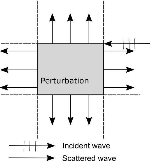
For 2DQW, the scattered wave does not spread radially as above. Since V=UU0V=U-U_{0} is finite rank, the scattered wave for every chirality passes along corridors. See Figure 3.

Theorem 4.20.

Let ϕ𝐡(θ)\phi\in{\bf h}(\theta).

  1. (1)

    (A(θ)ϕ)(x2)(A_{\leftarrow}(\theta)\phi)(x_{2}) and (A(θ)ϕ)(x2)(A_{\rightarrow}(\theta)\phi)(x_{2}) vanish for |x2|n0+1|x_{2}|\geq n_{0}+1.

  2. (2)

    (A(θ)ϕ)(x1)(A_{\downarrow}(\theta)\phi)(x_{1}) and (A(θ)ϕ)(x1)(A_{\uparrow}(\theta)\phi)(x_{1}) vanish for |x1|n0+1|x_{1}|\geq n_{0}+1.

As a consequence, A(θ)A(\theta) is an operator of finite rank.

Proof. Note that

v(+)=u(+)u(0)=eiθ(eiθR0(θi0)g+Vu(0)),v^{(+)}=u^{(+)}-u^{(0)}=e^{i\theta}\left(e^{i\theta}R_{0}(\theta-i0)g+V^{*}u^{(0)}\right),

where g=Vu(0)VR(θi0)Vu(0)g=V^{*}u^{(0)}-VR(\theta-i0)V^{*}u^{(0)} for u(+)=(+)(θ)ϕu^{(+)}=\mathcal{F}^{(+)}(\theta)^{*}\phi and u(0)=(0)(θ)ϕu^{(0)}=\mathcal{F}^{(0)}(\theta)^{*}\phi, ϕ𝐡(θ)\phi\in{\bf h}(\theta). In view of the assumption for C(x)C(x), we have (Vu(0))(x)=((C1)S1u(0))(x)=0(V^{*}u^{(0)})_{\leftarrow}(x)=((C^{*}-1)S^{-1}u^{(0)})_{\leftarrow}(x)=0 for |x2|n0|x_{2}|\geq n_{0}. Similarly, we have (VR(θi0)Vu(0))(x)=(S(C1)R(θi0)Vu(0))(x)=0(VR(\theta-i0)V^{*}u^{(0)})_{\leftarrow}(x)=(S(C-1)R(\theta-i0)V^{*}u^{(0)})_{\leftarrow}(x)=0 for |x2|n0|x_{2}|\geq n_{0}. Thus the formula (3.16) shows that v(+)(x)v^{(+)}(x) vanishes for |x2|0|x_{2}|\geq 0. This implies that (A(θ)ϕ)(x2)=0(A_{\leftarrow}(\theta)\phi)(x_{2})=0 for |x2|0|x_{2}|\geq 0. The proofs for Ap(θ)ϕA_{p}(\theta)\phi with p{,,}p\in\{\rightarrow,\downarrow,\uparrow\} are similar. ∎

References

  • [1] S. Agmon and L. Hörmander, Asymptotic properties of solutions of differential equations with simple characteristics, J. Anal. Math., 30 (1976), 1-30.
  • [2] W. O. Amrein, A. Boutet de Monvel, and V. Georgescu, “C0C_{0}-groups, commutator methods and spectral theory of NN-body Hamiltonians”, volume 135 of Progress in Mathematics, Birkhäuser Verlag, Basel, 1996.
  • [3] K. Ando, H. Isozaki and H. Morioka, Spectral properties of Schrödinger operators on perturbed lattices, Ann. Henri Poincaré, 17 (2016), 2103-2171.
  • [4] K. Ando, H. Isozaki and H. Morioka, Inverse scattering for Schrödinger operators on perturbed lattices, Ann. Henri Poincaré, 19 (2018), 3397-3455.
  • [5] E. Feldman and M. Hillery, Quantum walks on graphs and quantum scattering theory, Coding Theory and Quantum Computing, edited by D. Evans, J. Holt, C. Jones, K. Klintworth, B. Parshall, O. Pfister, and H. Ward, Contemporary Mathematics, 381 (2005), 71-96.
  • [6] E. Feldman and M. Hillery, Modifying quantum walks: A scattering theory approach, Journal of Physics A: Mathematical and Theoretical 40 (2007), 11343-11359.
  • [7] C. Fernández, S. Richard and R. Tiedra de Aldecoa, Commutator methods for unitary operators, J. Spectr. Theory, 3 (2013), 271-292.
  • [8] Yu. Higuchi and E. Segawa, Dynamical system induced by quantum walks, J. Phys. A: Math. Theor. 52 (2009) 395202.
  • [9] H. Isozaki and E. Korotyaev, Inverse problems, trace formulae for discrete Schrödinger operators, Ann. Henri Poincaré, 13 (2012), 513-542.
  • [10] H. Isozaki and H. Morioka, A Rellich type theorem for discrete Schrödinger operators, Inverse Problems and Imaging, 8 (2014), 475-489.
  • [11] H. Isozaki and H. Morioka, Inverse scattering at a fixed energy for discrete Schrödinger operators on the square lattice, Ann. l’Inst. Fourier, 65 (2015), 1153–1200.
  • [12] T. Komatsu, N. Konno, H. Morioka and E. Segawa, Generalized eigenfunctions for quantum walks via pass counting approach, Rev. Math. Phys., 33 (2021), 2150019, pp. 1-24.
  • [13] M. Maeda, H. Sasaki, E. Segawa, A. Suzuki and K. Suzuki, Scattering and inverse scattering for nonlinear quantum walks, Discrete and Continuous Dynamical Systems A, 38 (2018), 3687-3703.
  • [14] M. Maeda, H. Sasaki, E. Segawa, A. Suzuki and K. Suzuki, Dispersive estimates for quantum walks on 1D lattice, preprint. arXiv:1808.05714
  • [15] H. Morioka, Generalized eigenfunctions and scattering matrices for position-dependent quantum walks, Rev. Math. Phys., 31 (2019), 1950019, pp. 1-37.
  • [16] H. Morioka and E. Segawa, Detection of edge defects by embedded eigenvalues of quantum walks, Quantum Inf. Process., 18 (2019), 283, pp. 1-18.
  • [17] S. Nakamura, Microlocal properties of scattering matrices, Commn. PDE, 41 (2016), 894-912.
  • [18] S. Richard, A. Suzuki and R. Tiedra de Aldecoa, Quantum walks with an anisotropic coin I: spectral theory, Lett. Math. Phys., 108 (2018), 331-357.
  • [19] S. Richard, A. Suzuki and R. Tiedra de Aldecoa, Quantum walks with an anisotropic coin II: scattering theory, Lett. Math. Phys., First Online (2018), DOI:10.1007/s11005-018-1100-1.
  • [20] J. Sahbani, The conjugate operator method for locally regular Hamiltonians, J. Operator Theory, 38 (1997), 297-322.
  • [21] A. Suzuki, Asymptotic velocity of a position-dependent quantum walk, Quantum Inf. Process, 15 (2016), 103-119.
  • [22] Y. Tadano, Long-range scattering for discrete Schrödinger operators, Ann. Henri Poincaré, 20 (2019), 1439-1469.
  • [23] R. Tiedra de Aldecoa, Stationary scattering theory for unitary operators with an application to quantum walks, J. Funct. Anal., 279 (2020), 108704.
  • [24] D. Yafaev, “Mathematical Scattering Theory: General Theory”, Translations of Mathematical Monographs, Vol. 105 (American Mathematical Society, Providence, RI, 2009).
  • [25] D. Yafaev, On solutions of the Schrödinger equations with radiation condition at infinity, Adv. in Sob. Math., 7 (1991), 179-204.
  • [26] K. Yoshida, “Functional Analysis”, Springer, Berlin, 1966.