Asymptotic Security using Bayesian Defense Mechanism with Application to Cyber Deception
Abstract
This paper addresses the question whether model knowledge can guide a defender to appropriate decisions, or not, when an attacker intrudes into control systems. The model-based defense scheme considered in this study, namely Bayesian defense mechanism, chooses reasonable reactions through observation of the system’s behavior using models of the system’s stochastic dynamics, the vulnerability to be exploited, and the attacker’s objective. On the other hand, rational attackers take deceptive strategies for misleading the defender into making inappropriate decisions. In this paper, their dynamic decision making is formulated as a stochastic signaling game. It is shown that the belief of the true scenario has a limit in a stochastic sense at an equilibrium based on martingale analysis. This fact implies that there are only two possible cases: the defender asymptotically detects the attack with a firm belief, or the attacker takes actions such that the system’s behavior becomes nominal after a finite number of time steps. Consequently, if different scenarios result in different stochastic behaviors, the Bayesian defense mechanism guarantees the system to be secure in an asymptotic manner provided that effective countermeasures are implemented. As an application of the finding, a defensive deception utilizing asymmetric recognition of vulnerabilities exploited by the attacker is analyzed. It is shown that the attacker possibly withdraws even if the defender is unaware of the exploited vulnerabilities, as long as the defender’s unawareness is concealed by the defensive deception.
Bayesian methods, game theory, intrusion detection, security, stochastic systems.
1 Introduction
Societal monetary loss from cyber crime is estimated to be about a thousand billion USD per year presently, and even worse, a rising trend can be observed [1]. Another trend is that not only information systems but also control systems, which are typically governed by physical laws, are exposed to cyber threats as demonstrated by recent incidents [2, 3, 4, 5]. Deception is a key notion to predict the consequence of incidents. Rational attackers take deceptive strategies, i.e., the attacker tries to conceal her existence and even mislead the defender into taking inappropriate decisions. An example of deception is replay attacks, which hijacks sensors of the plant, eavesdrops the nominal data transmitted when the system is operated under normal conditions, and replays the observed nominal data during the execution of another damaging attack. A replay attack was executed in the Stuxnet incident, and it was an essential factor leading to serious damage in the targeted plant [6]. The incident suggests that prevention of deception is a fundamental requirement for secure system design.
Assuming the situation where an attacker might intrude into a control system where a defense mechanism is implemented, this paper addresses the following question: Can model knowledge guide the defender to appropriate decisions against attacker’s deceptive strategies? Specifically, we consider the case where the stochastic model of the control system, the vulnerability to be exploited, and the objective of the attacker are known. The setting naturally leads to Bayesian defense mechanisms, which monitor the system’s behavior and form a belief on the existence of the attacker using the model. If the system’s behavior is inconsistent with the nominal one, the belief increases owing to Bayes’ rule. When the belief is strong enough, the Bayesian defense mechanism proactively carries out a proper reaction. On the other hand, we also suppose a powerful attacker who knows the model and the defense scheme to be implemented. The attacker aims at achieving her objective while avoiding being detected by deceiving the defender.
For mathematical analysis, we formulate the decision making as a dynamic game with incomplete information. More specifically, we refer to the game as a stochastic signaling game, because it is a stochastic game [7] in the sense that the system’s dynamics is given as a Markov decision process (MDP) governed by two players and it is also a signaling game [8] in the sense that one player’s type is unknown to the opponent. In this game, the attacker strategically chooses harmful actions while avoiding being detected, while the defender, namely, the Bayesian defense mechanism, chooses appropriate counteractions according to her belief.
Based on the game-theoretic formulation, we find that model knowledge can always lead the defender to appropriate decisions in an asymptotic sense as long as the system’s dynamics admits no stealthy attacks. More specifically, there are only two possible cases: one is that the defender asymptotically forms a firm belief on the existence of an attacker and the other is that the attacker takes harmless actions after finite time such that the system converges to nominal behavior. This finding leads to the conclusion that the Bayesian defense mechanism guarantees the system to be secure in an asymptotic manner.
The analysis means that the defender always wins in an asymptotic manner when the stochastic model of the system is available and the vulnerability exploited for the intrusion is known and modeled. However, in practice, it is hard to be aware of all possible vulnerabilities in advance. As an application of the finding above, we consider defensive deception using bluffing that utilizes asymmetric recognitions between the attacker and the defender. Specifically, we suppose that, the defender is unaware of the exploited vulnerability but the attacker is unaware of the defender’s unawareness. If the state of the system does not possess any information about the defender’s recognition on the vulnerability, the attacker cannot identify whether the defender is aware of the vulnerability, or not. The result obtained in the former part suggests that the attacker may possibly withdraw if the defender’s reactions affect only the attacker’s utility without influence to the system’s behavior. The difficulty of the analysis is that standard incomplete information games, which assume common prior, cannot describe this situation. The common prior implicitly assumes that the attacker is aware of the defender’s unawareness. To overcome the difficulty, we employ the Mertens-Zamir model, which can represent incomplete information games without common prior assumption, using the notion of belief hierarchy [9, 10]. Based on this setting, we show, in a formal manner, that the defensive deception effectively works when the attacker strongly believes that the defender is aware of the vulnerability.
Related Work
Model-based security analysis helps the system designer to prioritize security investments [11]. Attack graphs [12] and attack trees [13] are basic models of vulnerabilities, attacks, and consequences. Incorporating defensive actions into the graphical representation induces defense trees [14]. For dynamic models, attack countermeasure trees, partially observable MDP, and Bayesian network model have been used [15, 16, 17]. Those probabilistic models naturally lead to Bayesian defense mechanisms, such as Bayesian intrusion detection [18, 19], Bayesian intrusion response [20], and Bayesian security risk management [21]. Meanwhile, the model of the dynamical system to be protected is also used for control system security [22, 23]. For example, identifying existence of stealthy attacks and removing the vulnerability require the dynamical model [24, 25], and attack detection performance can be enhanced by model knowledge [26]. Our Bayesian defense mechanisms can be interpreted as a generalization of those approaches. This work reveals a fundamental property of such commonly used model-based defense schemes.
Game theory is a standard approach to modeling the decision making in cyber security, where there inevitably arises a need to address strategic interactions between the attacker and the defender [27, 28]. In particular, games with incomplete information play a crucial role in deceptive situations [29, 30, 31, 32]. The modeling in this study follows the signaling game framework in [33, 34]. Our main concern is especially on asymptotic phenomena in the dynamic deception and effectiveness of model knowledge.
Our finding is based on analysis of an asymptotic behavior of Bayesian inference. The convergence property of Bayesian inference on the true parameter is referred to as Bayesian consistency, which has been investigated mainly in the context of statistics [35, 36]. However, those existing results are basically applicable only to independent and identically distributed (i.i.d.) samples because the discussion mostly relies on the strong law of large numbers (SLLN). Although there is an extension to Markov chains [37], the observable variable in our work is not Markov. Indeed, sophisticated attackers can choose strategies such that the states at all steps are correlated with the entire previous trajectory. Thus, existing results for Bayesian consistency cannot be applied to our problem in a straightforward manner.
Organization and Preliminaries
In Section 2, we present a motivating example of water supply networks, and subsequently, formulate the decision making as a stochastic signaling game. Section 3 analyzes the consequence of the formulated game and shows that Bayesian defense mechanisms can achieve asymptotic security of the system to be protected. In Section 4, we analyze a defensive deception that utilizes asymmetric recognition as an application of the finding of Section 3. The game of interest is reformulated using the Mertens-Zamir model. It is shown that the attacker possibly stops the execution even if the defender is unaware of the exploited vulnerabilities, as long as the defender’s belief is concealed. Section 5 verifies the theoretical results through numerical simulation. Finally, Section 6 concludes and summarizes the paper.
Let , , and be the sets of natural numbers, nonnegative integers, and real numbers, respectively. The -ary Cartesian power of the set is denoted by The tuple is denoted by . The cardinality of a set is denoted by . For a set the Kronecker delta denoted by is defined by if and otherwise. The -algebra generated by a random variable is denoted by . For a sequence of events for , the supremum set , namely, the event where occurs infinitely often, is denoted by . Jensen’s inequality, which is often applied in this paper, is given as follows: For a real convex function and a finite set , the inequality
| (1) |
holds where and that satisfies the equation . The inequality is reversed if is concave. The generalized Borel-Cantelli’s second lemma is given as follows [40, Theorem 4.3.4]: Let for be a filtration of a probability space with and let for be a sequence of events with . Then
| (2) |
The appendix contains the proofs of the claims made in the paper.
2 Modeling using Stochastic Signaling Games
2.1 Motivating Example
As a motivating example, we consider water distribution networks (WDNs), which supply drinking water of suitable quality to customers. Because of their indispensability to our life, WDNs are an attractive target for adversaries and expose their architecture to cyber-physical attacks [41]. In particular, we treat the water tank system illustrated by Fig. 1, where a tank is connected to a reservoir within a WDN. The amount of the water in the tank varies due to usage for drinking and flow between the external network. Thus the tank system is needed to be properly controlled through actuation of the pump and the valve to keep the water amount within a desired range [42]. A programmable logic controller (PLC) transmits on/off control signals to the pump and the valve monitoring the state, namely, the water level of the tank. The dynamics is modeled as a MDP, where the state space and the action space are given by quantized water levels and finite control actions. Interaction to the external network is modeled as the randomness in the process.
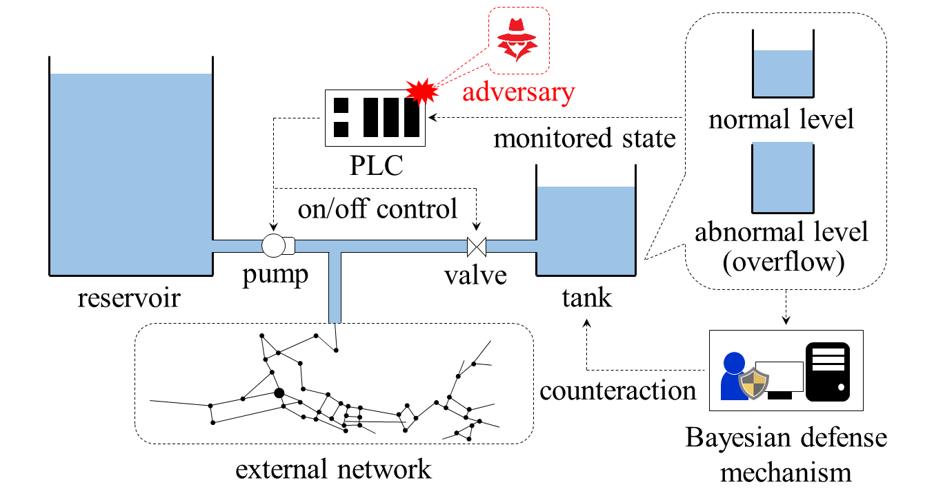
We here suppose an attack scenario considered in [43]. The adversary succeeds to hijack the PLC and can directly manipulate its control logic. Such an intrusion can be carried out by stealthy and evasive maneuvers in advanced persistent threats [44]. The objective of the attack is to damage the system by causing water overflow through inappropriate control signals without being detected. To deal with this attack, we consider a Bayesian defense mechanism, which utilizes the data of the monitored state and forms her belief on existence of the attacker based on the system model. The Bayesian defense mechanism chooses a proper reaction by identifying if the system is under attack through an observation of the state. If the system’s behavior is highly suspicious, for example, the defense mechanism takes an aggressive reaction such as log analysis, dispatch of operators, or emergency shutdown.
The defender’s belief on the existence of an attacker plays a key role to analyze the consequence of the threat. When the attacker naively executes an attack, the system’s behavior becomes different from the one of the normal operation and accordingly the belief increases. On the other hand, if the attacker chooses sophisticated attacks that deceive the defender, the belief may decrease. Our main interest in this study is to investigate the defense capability achieved by the Bayesian defense mechanism.
2.2 Modeling using Stochastic Signaling Game
We introduce the general description based on dynamic games with incomplete information. In particular, we refer to the game as a stochastic signaling game where the system’s dynamics is given as an MDP and the type of a player is unknown to the opponent.
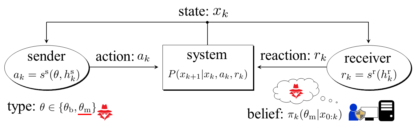
The system to be protected with a Bayesian defense mechanism is depicted in Fig. 2. The system is modeled by a finite MDP governed by two players as in standard stochastic games. Formally, the MDP considered in this paper is given by the tuple where is a finite state space, and are finite action spaces, is a transition probability, and is the probability distribution of the initial state. The state at the th step is denoted by . There is an agent who can alter the system through an action for . We refer to the agent as sender as in standard signaling games. Based on the measured output, the Bayesian defense mechanism, called a receiver, chooses an action at each time step. We henceforth refer to as a reaction for emphasizing that denotes a counteraction against potentially malicious attacks. The system dynamics is given by , where the transition probability from to with and is denoted by . To eliminate the possibility of trivial stealthy attacks, we assume that the system’s behavior varies in a stochastic sense when different actions are taken.
Assumption 1
For any and , there exists such that
| (3) |
for different actions .
Next, we determine the class of the decision rules. Let denote the type of the sender. For simplicity, the type is assumed to be binary, i.e., where and correspond to benign and malicious senders, respectively. The types and describe the situations where there does not and does exist an adversary, respectively. The true type is known to the sender, but unknown to the receiver. Let and denote the sender’s and receiver’s pure strategy, respectively. It is assumed that the receiver’s available information about the sender type is only the state, i.e., she cannot observe her instantaneous utility, defined below, nor the sender’s action. Similarly, it is assumed that the sender can observe only the state and her action. The strategies at the th step with the available information are given by and where and are histories at the th step given by and Note that the resulting state trajectory is not Markov since the strategies depend on the entire history. Because we consider pure strategies, it suffices to consider the state-history dependent strategies and , recursively defined by
| (4) |
The strategy profile is denoted by The sender’s and receiver’s admissible strategy sets are denoted by and , respectively. The set of admissible strategy profiles is denoted by . Note that, although we do not specify here, it can be taken to be any set of state-history dependent strategies. While we consider a general strategy set in Sec. 3, we impose a constraint on in Sec. 4.
Once a strategy profile is fixed, the stochastic property of the system is induced. Construct the canonical measurable space of the MDP with the sender type where and is its product -algebra [45, Chapter 2]. We denote . The random variables and are defined on the measurable space by the projections of such that The probability measure on , induced by , is denoted by , which satisfies
| (5) |
for any with the initial distribution of the sender type . We denote the conditional probability by . To simplify the notation, we denote the conditional probability mass function with type by
| (6) |
The expectation with respect to is denoted by .
We introduce each player’s belief on the uncertain variables next. The receiver’s belief at the th step is given by
| (7) |
for . The belief can be recursively computed by Bayes’ rule
| (8) |
when the denominator is nonzero. To simplify notation, we introduce the receiver’s belief only of the sender type:
| (9) |
which follows Bayes’ rule
| (10) |
The sender’s belief can similarly be defined and is denoted by .
In Sec. 3, the initial beliefs are assumed to be known to both players, i.e., we make the common prior assumption. Since we consider pure strategies, is uniquely determined by once the strategy is fixed. Hence, the sender’s belief does not appear explicitly in Sec. 3. On the other hand, in Sec. 4, we consider the case where the initial belief is unknown to the sender, modeling the possibility of bluffing.
Let be the sender’s instantaneous utility. For a given strategy profile and type , the sender’s expected average utility at the th step with the horizon length is given by
| (11) |
Similarly, with the receiver’s instantaneous utility given by , the receiver’s expected average utility at the th step with the horizon length is given by
| (12) |
We denote the limits by assuming they exist. Under this notation, the strategy profile is said to be a perfect Bayesian equilibrium (PBE) if
| (13) |
for any and where and are best responses defined by
| (14) |
Note that, our analysis can be extended to the case of general objective functions rather than expected average utilities as long as the adversary with the utilities avoids being detected, which is formally stated in Definition 1 below.
We define the game formulated above by
| (15) |
where the initial belief is common information. This game belongs to the class of incomplete, imperfect, and asymmetric information stochastic games. Owing to the existence of the type which is unknown to the receiver, the information is incomplete. Because the actions taken by each player are unobservable to the opponent, the information is imperfect and asymmetric. Although investigating existence and computing equilibria of the game are challenging, we discuss properties of equilibria on the premise that they exist and are given because our interest here lies in the consequences for the threat.
3 Analysis: Asymptotic Security
In this section, we analyze asymptotic behaviors of beliefs and actions when the adversary avoids being detected. It is shown that the system is guaranteed to be secure in an asymptotic manner as long as the defender possesses an effective counteraction.
3.1 Belief’s Asymptotic Behavior
The random variable of the belief on the type at the th step is given by
| (16) |
Recall that represents the defender’s confidence on existence of an attacker. If the belief is low in spite of existence of malicious signals, this means that the Bayesian defense mechanism is deceived. Because we are interested in whether the Bayesian defense mechanism is permanently deceived, or not, we examine asymptotic behavior of the belief.
We first investigate increment of the belief sequence. The following lemma is key to our analysis.
Lemma 1
Consider the game . The belief of the true type is a submartingale with respect to the probability and the filtration for any type and strategy profile .
Lemma 1 roughly implies that the expectation of the belief on the true type is non-decreasing. As a direct conclusion of this lemma, the following theorem holds.
Theorem 1
Consider the game . There exists an integrable random variable such that
| (17) |
for any type and strategy profile .
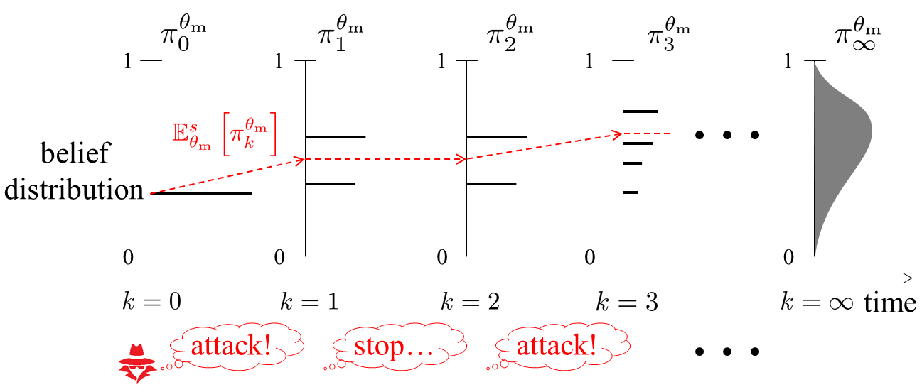
Theorem 1 implies that the belief has a limit even if an intermittent attack is executed. Fig. 3 depicts the distributions of the belief sequence when there exists an attacker. Owing to the model knowledge, if the adversary stops the attack at some time step then the belief is invariant, which is illustrated as the transition of the belief at in Fig. 3. Moreover, the expectation of the belief is non-decreasing over time as claimed by Lemma 1. Thus, there exists a limit as shown at the right of Fig. 3.
We next investigate the limit. An undesirable limit is , which means that the defender is completely deceived. We show that this does not happen as long as the initial belief is nonzero. The following lemma holds.
Lemma 2
Consider the game . If for any type then with any basis converges -almost surely to an integrable random variable as for any type and strategy profile .
Lemma 2 leads to the following theorem.
Theorem 2
Consider the game . If then
| (18) |
for any type and strategy profile .
Theorem 2 implies that the complete deception described by does not occur.
Remark: Theorems 1 and 2 can heuristically be justified from an information-theoretic perspective as follows. Suppose that the state sequence is observed at the th step. Then the belief is given by
| (19) |
where and are the joint probability mass functions of with respect to and , respectively, and
| (20) |
Assuming that approaches a stationary distribution on and SLLN can be applied, we have
| (21) |
where denotes the Kullback-Leibler divergence. Since is nonnegative for any pair of distributions, converges to a nonpositive number, which results in convergence of . If for any , the limit of becomes negative, and hence which leads to
| (22) |
Thus, the belief of the true type converges to one. Such a convergence property of the Bayesian estimator on the true parameter, referred to as Bayesian consistency, has been investigated mainly in the context of statistics [35, 36]. In this sense, Theorems 1 and 2 can be regarded as another representation of Bayesian consistency. However, note again that this discussion is not a rigorous proof but a heuristic justification because the state is essentially non-i.i.d. and even non-ergodic in our game-theoretic formulation.
3.2 Asymptotic Security
It has turned out that the belief has a positive limit. To clarify our interest, we define the notion of detection-averse utilities.
Definition 1
(Detection-averse Utilities) A pair in the game are detection-averse utilities when
| (23) |
for any PBE .
Definition 1 characterizes utilities where the malicious sender avoids having the defender form a firm belief on the existence of an attacker. An example of detection-averse utilities is given in Appendix 7. Naturally, strategies reasonable for the attacker should be detection-averse as long as the defender possesses an effective counteraction. If the utilities of interest are not detection-averse, this means that the defense mechanism cannot cope with the attack because the attacker is not afraid to reveal herself. For protecting such systems, appropriate counteractions should be implemented beforehand.
Suppose that there is an effective countermeasure, and hence the utilities are detection-averse. A simple malicious sender’s strategy that satisfies (23) is to imitate the benign sender’s strategy after a finite number of time steps. We give a formal definition of such strategies.
Definition 2
(Asymptotically Benign Strategy) A strategy profile in the game is asymptotically benign when
| (24) |
where is the action taken by the sender with the type defined by
The objective of this subsection is to show that Bayesian defense mechanisms can restrict all reasonable strategies to be asymptotically benign as long as an effective countermeasure is implemented.
As a preparation for proving our main claim, we investigate the asymptotic behavior of state transition. From Theorems 1 and 2, we can expect that the state eventually loses information on the type, which is justified by the following lemma.
Lemma 3
Consider the game with detection-averse utilities. If then
| (25) |
for any PBE .
Under Assumption 1, which eliminates the possibility of stealthy attacks, Lemma 3 implies that the actions themselves must be identical. This fact yields the following theorem, one of the main results in this paper.
Theorem 3
Consider the game with detection-averse utilities. Let Assumption 1 hold and assume . Then, every PBE of is asymptotically benign.
Theorem 3 implies that the malicious sender’s action converges to the benign action. Equivalently, an attacker necessarily behaves as a benign sender after a finite number time steps. Therefore, the system is guaranteed to be secure in an asymptotic manner, i.e., Bayesian defense mechanisms can prevent deception in an asymptotic sense. This result indicates the powerful defense capability achieved by model knowledge.
4 Application: Analysis of Defensive Deception utilizing Asymmetric Recognition
4.1 Idea of Defensive Deception using Bluffing
The result in Section 3 claims that the defender, namely, the Bayesian defense mechanism, always wins in an asymptotic manner when the stochastic model of the system is available and the vulnerability to be exploited for intrusion is known and modeled. The latter condition is quantitatively described by the condition . Although the derived result proves a quite powerful defense capability, it is also true that it is almost impossible to be aware of all possible vulnerabilities in advance. Moreover, it is also challenging to implement effective countermeasures for all scenarios and to compute the equilibrium of the dynamic game.
In this section, as an application of the finding in the previous section, we consider defensive deception using bluffing that utilizes asymmetric recognitions between the attacker and the defender. Suppose that an attacker exploits a vulnerability of which the defender is unaware but the attacker is unaware of the defender’s unawareness. Then their recognition becomes asymmetric in the sense that the attacker does not correctly recognize the defender’s recognition of the vulnerability. This situation naturally arises in practice because the defender’s recognition is private information. By utilizing the asymmetric recognition, the defender can possibly deceive the attacker such that the attacker believes that the defender might be aware of the vulnerability and carrying out effective counteractions. Specifically, we consider the bluffing strategies where the system’s state does not possess information about the defender’s belief. For instance, if the defender chooses the reactions that affect only the players’ utilities without influence to the system, the state is independent of the reaction. By concealing the defender’s unawareness, the defender’s recognition, which is quantified by her belief, is completely unknown to the attacker over time.
The defensive deception is possibly able to force the attacker to withdraw even if the defender is actually unaware of the exploited vulnerability. For instance, consider the example in Sec. 2.1 and suppose that emergency shutdown of the system can be carried out by the defender. Suppose also that the attacker wants to keep administrative privileges of the PLC. In this case, the attacker may rationally terminate her evasive maneuvers after a finite number of time steps due to the risk of sudden shutdown. The objective of this section is to show that the hypothesis is true in a formal manner.
4.2 Reformulation using Type Structure
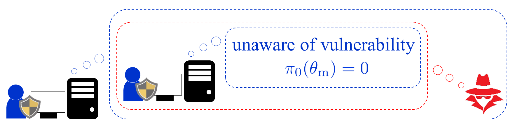
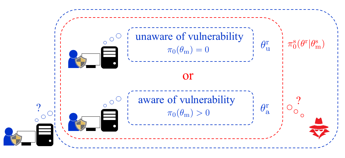
The situation of interest in this section is that the defender is unaware of the vulnerability to be exploited but the attacker is not necessarily aware of this unawareness. To address the uncertainty on defender’s recognition, the attacker forms her belief on the defender’s belief. Fig. 4 illustrates the attacker’s belief on the defender’s belief with the common prior assumption, i.e., the initial defender’s belief is known to the attacker, which has been made in the previous section. In this case, the attacker has a firm belief that the defender is unaware of the vulnerability. On the other hand, Fig. 5 illustrates the attacker’s belief without the common prior assumption. Then the attacker’s belief is no longer firm as depicted by the figure. In addition, because of the lack of the common prior assumption, the defender also forms another belief on the attacker’s belief on the defender’s belief on the existence of an attacker. This procedure repeats indefinitely and induces infinitely many beliefs.
The notion of belief hierarchy has been proposed to handle the infinitely many beliefs [9, 10, 46]. A belief hierarchy is formed as follows. Let denote the set of probability measures over a set. The first-order initial belief is given as , which describes the defender’s initial belief on existence of the attacker. The second-order initial belief is given as , which describes the attacker’s initial belief on the defender’s first-order belief. In a similar manner, the belief at any level is given, and the tuple of beliefs at all levels is referred to as a belief hierarchy.
To handle belief hierarchies, the Mertens-Zamir model has been introduced [9, 10, 46]. The model considers type structure, in which a belief hierarchy is embedded. A type structure consists of players, sets of types, and initial beliefs. In particular, a type structure for our situation of interest can be given by
| (26) |
where represents the sender and the receiver, and represent the sets of player types, and and represent the initial beliefs. The value denotes the sender’s initial belief of the receiver type when the sender type is , and denotes the corresponding receiver’s initial belief. The first-order initial belief is given by for the true receiver type , and the second-order initial belief is given by for the true sender type . By repeating it, the belief at any level of the belief hierarchy can be derived from the type structure. Importantly, for any reasonable belief hierarchy there exists a type structure that can generate the belief hierarchy of interest. For a formal discussion, see [9, 10, 46].
We model the situation of interest by using the binary type sets:
| (27) |
While and represent benign and malicious senders, respectively, and represent receivers being unaware and aware of the vulnerability, respectively. The receiver’s initial beliefs are set to
| (28) |
and
| (29) |
with . The initial beliefs mean that, the receiver is unaware of the vulnerability and firmly believes that the system is normally operated, while the receiver is aware of the vulnerability and suspects existence of an attacker with probability . The sender’s initial beliefs are assumed to be given by
| (30) |
and
| (31) |
with . The malicious sender does not know the true receiver type, i.e., whether the sender is aware of the vulnerability or not. The given initial beliefs are summarized in Table 1.
| 1 | 0 | |
| 1 | 0 | |
In accordance with the introduction of the type structure, the definition of strategies and the solution concept are needed to be slightly modified. The contrasting ingredients of the game with symmetric recognition and the one with asymmetric recognition are listed in Table 2, where those with asymmetric recognition can analogically be defined. The conditional probability , which is the probability measure induced by and , is denoted by . The sender’s expected average utility at the th step with the horizon length is given by
| (32) |
The receiver’s expected average utility at the th step with the horizon length is given by
| (33) |
A strategy is said to be a PBE when the limit of the utilities satisfies
| (34) |
for any and where
| (35) |
| symmetric recognition | asymmetric recognition | |
|---|---|---|
| receiver’s strategy | ||
| sender’s belief | N/A | |
| receiver’s belief | ||
| sender’s utility | ||
| receiver’s utility |
We define the game formulated above by
| (36) |
where the defender’s initial belief is not common information in contrast to .
In the following discussion, we analyze through . To clarify their relationship, we describe the game using the modified formulation. Define another game
| (37) |
where
| (38) |
The initial belief means that the adversary believes that the defender is aware of the vulnerability. The situation of is the same as that of if the defender is aware of the vulnerability. Thus, these games lead to the same consequence when the true types are and . The following lemma holds.
Lemma 4
Consider the games and . For a strategy profile in , let be a strategy profile in such that
| (39) |
where is the restriction of with . Then the probability measures induced by and are equal when and , i.e.,
| (40) |
Also, if then .
We extend the notions of detection-averse utilities and asymptotically benign strategies to . Our objective is to investigate the effectiveness of the proposed defensive deception. It is possible to define detection-averse utilities directly using the game as utilities where the resulting equilibrium leads the adversary to avoid being detected. However, this definition immediately means that the defensive deception works well, and any results from the definition cannot show its effectiveness. Instead, we say that utilities in are detection-averse when the adversary avoids being detected if she is certain that the defender is aware of the vulnerability.
Definition 3
(Detection-averse Utilities in ) A pair of utilities in the game are detection-averse utilities when
| (41) |
for any PBE of .
Note that Definition 3 is a necessary requirement to make the game interesting, because the adversary is not afraid of being detected at all without this condition.
Next, we define desirable strategies that should be achieved by Bayesian defense mechanisms. We say a strategy in to be asymptotically benign when it becomes benign regardless of the defender’s awareness.
Definition 4
(Asymptotically Benign Strategies in ) A strategy profile in the game is asymptotically benign when
| (42) |
for any .
Note that Definition 4 requires the strategy to be asymptotically benign for any . In other words, the strategy is needed to be asymptotically benign even if the defender is unaware of the vulnerability.
4.3 Passively Bluffing Strategies
We expect that there exists a chance of preventing attacks that exploit unnoticed vulnerabilities if the state does not possess information about the defender’s recognition. To formally verify this expectation, we define passively bluffing strategies.
Definition 5
(Passively Bluffing Strategies) A strategy profile in is a passively bluffing strategy profile when the sender’s belief satisfies
| (43) |
for any and . A strategy profile set in is a passively bluffing strategy set when its all elements are passively bluffing.
Definition 5 requires the sender’s belief to be invariant over time. If the strategy is passively bluffing, the adversary cannot identify whether the defender is aware of the exploited vulnerability or not even in an asymptotic sense. Note that the introduced passively bluffing strategies can be regarded as a commitment. It is well known that restricting feasible strategies, referred to as commitment, can be beneficial in a game [47, 48]. In what follows, we investigate the effectiveness of the specific commitment.
Passively bluffing strategies can relax the condition for asymptotically benign strategies. The following lemma holds.
Lemma 5
Consider the game . If a passively bluffing strategy profile satisfies
| (44) |
then is asymptotically benign.
The difference between (42) and (44) is the required receiver type. Lemma 5 implies that if a passively bluffing strategy profile is asymptotically benign when the receiver is aware of the vulnerability then the strategy is needed to be asymptotically benign even when the receiver is unaware of the vulnerability.
Remark: Although Definition 5 depends not only on the receiver’s strategy but also on the sender’s strategy for generality, the bluffing should be realized only by the defender in practice. A simple defender’s approach to achieving the bluffing is to choose reactions that do not influence the system’s behavior. Let be the set of reactions such that the system’s dynamics is independent of the reaction, i.e., the transition probability satisfies
| (45) |
for any , , , . If the receiver’s strategy takes only reactions in every strategy profile is passively bluffing. Indeed, because the transition probability is independent of , the probability distribution of the state is independent of . Thus, from Bayes’ rule, we have
| (46) |
when . An example of such reactions is just analyzing the network log and raising an alarm inside the operation room without applying control on the system itself. Note that the reaction still affects the players’ decision making through their utility functions, even if (45) holds.
4.4 Analysis
Our expectation can be described in a quantitative form based on the definition of passively bluffing strategies, which lead to a simple representation of the sender’s utility. If is passively bluffing, the sender’s belief is invariant over time. Hence, the sender’s utility with infinite horizon is given by
| (47) |
where
| (48) |
Note that and denote the sender’s utilities of the two cases where the defender is aware and unaware of the vulnerability, respectively. Thus (47) implies that the sender’s utility is simply given as a sum weighted by her initial beliefs when the strategy is passively bluffing. Therefore, we can expect that the sender possibly stops the execution in the middle of the attack if is sufficiently large. We show the existence of such sender’s initial belief. Note that is the trivial case, and thus we assume that sender’s initial beliefs that are strictly less than one.
First, we rephrase the result in Sec. 3. Let denote the set of non-asymptotically-benign strategies in . Our aim here is to show that the set of PBE of does not overlap with when the attacker strongly believes that the defender is aware of the vulnerability. It suffices to show that there is no overlap between the set of PBE of and where
| (49) |
where the benign sender and the receiver with any type take their best response strategies. Note that, and of the games and are identical because the sets are independent of the malicious sender’s belief. The following lemma is another description of the claim of Theorem 3 with respect to and .
Lemma 6
Consider the game with detection-averse utilities. Let Assumption 1 hold. For any strategy profile in , there exists such that
| (50) |
holds where
| (51) |
Lemma 6 implies the existence of a function
| (52) |
for any Thus we have where
| (53) |
We here make an assumption that is uniformly lower bounded by a positive value.
Assumption 2 eliminates the case where the difference between the sender’s utilities achievable by asymptotically benign strategies and non-asymptotically-benign strategies is infinitesimally small.
The following theorem, the main result of this section, holds.
Theorem 4
Theorem 4 implies that the system can possibly be protected by passively bluffing strategies if the attacker strongly believes that the defender is aware of the vulnerability. The result suggests the importance of concealing the defender’s recognition and the effectiveness of defensive deception.
5 Simulation
In this section, we confirm the theoretical results through numerical simulation.
5.1 Fundamental Setup
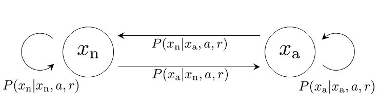
We assume the state space and the action space to be binary, i.e., and The states and represent the normal and abnormal states, respectively, and and represent benign and malicious actions, respectively. The benign and malicious actions correspond to nominal and malicious control signals, respectively. The reaction set is given by . The state transition diagram is depicted in Fig. 6. The initial state is set to . The transition probability is given as follows. Set the transition probability from to be given by
| (54) |
for any , which means that the probability from the normal state to the abnormal state is increased by the malicious action and it is independent of the reaction. The transition probability from to is given by Table 3. The probability from the abnormal state to the abnormal state is increased by the malicious action and it is decreased by the reaction . The reaction corresponds to bluffing since it induces the same transition probability as .
| 0.5 | 0.3 | 0.5 | |
| 0.6 | 0.4 | 0.6 |
The utilities are given as follows. The benign sender’s utility is
| (55) |
for any and , which means that the benign sender prefers the nominal state regardless of other variables. The malicious sender’s utility is given by Table 4. The benign action is a risk-free action, which always induces zero utility, while the malicious action is a risky action. If the reaction is the malicious sender obtains positive utility, where the abnormal state is more preferred than . On the other hand, if the reaction is the malicious sender incurs loss. The receiver’s utility is set to be independent on and given by Table 5, where is omitted. The receiver obtains utility only when she takes an appropriate reaction depending on the sender type. When an appropriate reaction is chosen, the normal state is more preferred than the abnormal state. Note that induces the same utilities as those with but it increases the probability of the abnormal state. Therefore, there is no motivation to choose when the defender’s recognition is known to the attacker.
| 0 | 0 | 0 | |
| 0 | 0 | 0 |
| 1 | -3 | -3 | |
|---|---|---|---|
| 2 | -3 | -3 |
| 5 | 0 | 0 | |
| 1 | 0 | 0 |
| 0 | 5 | 5 | |
| 0 | 1 | 1 |
Since it is difficult to compute an exact equilibrium for the infinite time horizon problem, we treat a sequence of equilibria for a finite time horizon problem as a tractable approximation [49]. Letting be the resulting equilibrium of the finite time horizon game, we use and as the th strategies as with receding horizon control. The equilibrium is obtained through brute-force search. For the game , the strategies in the simulation are given in a similar manner. The horizon length is set to . In the numerical examples, the equilibrium is uniquely determined.
5.2 Simulation: Asymptotic Security
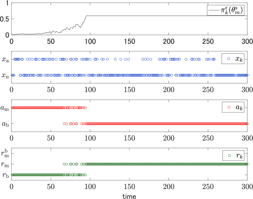
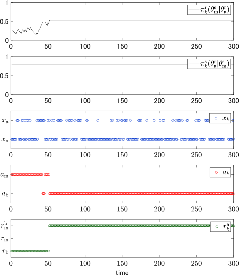
In the first scenario, we consider the case where the vulnerability is known, and thus this situation corresponds to the game in (15). The initial belief is given by , which is known to the sender. The true sender type is given by .
Under the setting, sample paths of the belief on the malicious sender, the state, the action, and the reaction with are depicted in Fig. 7. The belief converges to a nonzero value over time as claimed by Theorems 1 and 2. The action converges to the benign action as claimed by Theorem 3. The graphs evidence asymptotic security achieved by the Bayesian defense mechanism. In more detail, it can be observed that the malicious sender takes the malicious action while the receiver takes the reaction until about the time step . This is because the receiver’s belief on the malicious sender is low during the beginning of the game. On the other hand, between the time steps and , and sporadically appear because the belief is increased. Finally, after the time step , the belief exceeds a threshold, which results in the fixed actions and . It is notable that is not chosen at all since there is no reason for it, as explained above.
5.3 Simulation: Defensive Deception using Bluffing
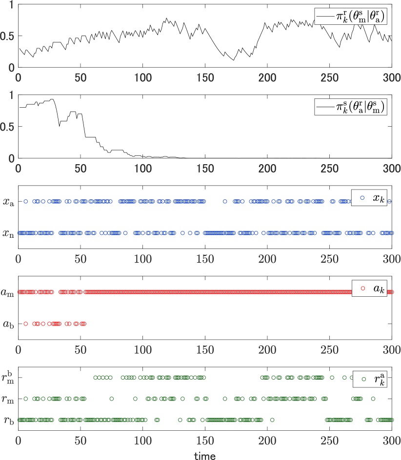
In the second scenario, we consider the case where the defender is unaware of the vulnerability and the attacker is unaware of the defender’s unawareness. Then this situation corresponds to the game in (36). The initial beliefs are given by and The true types are given by and . Note that and hence the defender is completely unaware of the attack while the game is proceeding.
We first consider the case where the strategy is not passively bluffing. The same transition probability as that used in the previous simulation, where it depends on the receiver’s reaction. As a result, the state possesses information about the receiver type.
Fig. 8 depicts sample paths of the receiver’s belief on the malicious sender if the receiver were aware of the vulnerability, the sender’s belief on the receiver being aware, the actual state, the actual action, and reactions that would be taken by the receiver being aware. It can be observed that the sender’s belief converges to zero, i.e., the sender notices that the receiver is unaware of the vulnerability. As a result, malicious actions are constantly taken after a sufficiently large number of time steps. The result indicates that the defense mechanism fails to defend the system in this case.
We next consider the bluffing case. As a commitment for passively bluffing strategy, we restrict the reaction set to . Then the transition probability is independent of the reaction, and hence any strategy becomes passively bluffing.
Fig. 9 depicts sample paths of those depicted in Fig. 8 under the bluffing setting. The sender’s belief is invariant over time because the state does not possess information about the receiver type. Thus, the malicious sender remains cautious about being detected. As a result, the benign action is continuously taken after a sufficiently large number of time steps in contrast to Fig. 8. The result indicates that asymptotic security is achieved by the bluffing even if the defender is unaware of the vulnerability. The simulation suggests importance of concealing the defender’s belief even if it degrades control performance.
6 Conclusion
This study has analyzed defense capability achieved by Bayesian defense mechanisms. It has been shown that the system to be protected can be guaranteed to be secure by Bayesian defense mechanisms provided that effective countermeasures are implemented. This fact implies that model knowledge can prevent the defender from being deceived in an asymptotic sense. As a defensive deception utilizing the derived asymptotic security, bluffing utilizing asymmetric recognition has been considered. It has also been shown that the attacker possibly stops the execution in the middle of the attack in a rational manner when she strongly believes the defender to be aware of the vulnerability, even if the vulnerability is unnoticed.
Important future work includes an extension to infinite state spaces because the state space in control systems typically is a subset of the Euclidean space. For this purpose, existing Bayesian consistency analysis for general sample space should be useful [36]. Moreover, although it is assumed that the state is observable in this framework, a generalization to partially observable setting is a more practical setting. We expect that the key properties such as Lemma 1 still holds if the system requirement, such as Assumption 1, can be appropriately modified. Another direction is to extend the results to non-binary types. Finally, finding a general condition for detection-averse utilities is an important issue. For this purpose, the example in Appendix 7 should be helpful.
7 Example of Detection-averse Utilities
Consider an MDP with binary spaces and . The initial state is and it goes to with probability when and stays at otherwise. The objective of the receiver is to detect the true state, which is modeled by
| (56) |
The malicious sender’s utility is given by
| (57) |
which means that the adversary wants to avoid being detected. The benign sender is assumed to choose anytime. The initial belief satisfies . Let be a strategy such that with probability . Take such and then there exists such that for any since
| (58) |
The receiver’s best response at is to take , which leads to the sender’s average utility at equal . Thus, the sender’s average utility at the initial state is . However, if the sender takes the strategy such that for any , then the sender’s average utility at the initial state is . Thus, is not a best response to , which means that the utilities are detection-averse.
8 Proofs of Propositions
In the proofs, we omit the symbol in the notation for simplicity when no confusion arises.
Proof.
Proof of Lemma 1: It is clear that is adapted to the filtration . It is also clear that is integrable with respect to since it is bounded. Thus, it suffices to show
| (59) |
for the claim. For a fixed outcome with which , the inequality is equivalent to
| (60) |
Thus it suffices to show (60) for any and .
Proof.
Proof.
Proof of Lemma 2: Since , we have -almost surely for any . Thus is well-defined. We first show that is a submartingale with respect to the probability measure and the filtration . It is clear that is adapted to the filtration . Because the number of elements in the support of is finite, is integrable for any . Thus it suffices to show that
| (68) |
As in the proof of Lemma 1, this inequality is equivalent to
| (69) |
for any . With the notation (63), this is equivalent to
| (70) |
Because the left-hand side can be rewritten by
| (71) |
the inequality (70) is equivalent to
| (72) |
which is also equivalent to
| (73) |
By applying Jensen’s inequality for a concave function with and we have
| (74) |
which implies that is a submartingale.
From Doob’s convergence theorem [50, Theorem 4.4.1], it suffices to show that the expectation of the nonnegative part of is uniformly bounded. Because , is nonpositive for any , and hence the uniform boundedness holds. ∎
Proof.
Proof of Theorem 2: We prove the claim by contradiction. Define as the inverse image of for . Assume that . For any as . Hence, from the continuity of logarithm functions, it turns out that as . This means that diverges for . However, Lemma 2 states that converges -almost surely. This is a contradiction. ∎
Proof.
Proof of Lemma 3: We first show that the coefficient of Bayes’ rule converges to one, i.e.,
| (75) |
where . Because is nonzero -almost surely from Theorem 2, we have
| (76) |
-almost surely. Thus (75) holds.
It is observed that can be calculated by
| (77) |
from (10). Define
| (78) |
which denote the numerator and the denominator of the coefficient , respectively. Since , we have for any . Thus
| (79) |
for any . Because from (75), the squeeze theorem for (79) yields
| (80) |
Now we have
| (81) |
Since is a PBE with detection-averse utilities, Therefore, (80) leads to the claim. ∎
Proof.
Proof of Theorem 3: From the definition of the conditional probability mass function, we have
| (82) |
Thus the claim of Lemma 3 can be rewritten by
| (83) |
-almost surely as . From finiteness of the MDP, the condition (83) is equivalent to
| (84) |
where
| (85) |
By applying the generalized Borel-Cantelli’s second lemma in (2) with we have
| (86) |
where
| (87) |
We derive a simpler description of the event . For any , the set of nonnegative integers can be divided into two disjoint subsets and such that
| (88) |
For a fixed , for . Thus we have
| (89) |
Moreover, for any and , we have
| (90) |
where
| (91) |
with and . Thus, the condition in the definition of can be rewritten by
| (92) |
Now we define We show the claim by contradiction. Assume . Then is well-defined. From (86), we have Because is assumed to be nonzero, this equation implies We now calculate from its definition. Let
| (93) |
For any , the set is nonempty for from Assumption 1. This fact and the finiteness of the MDP lead to that The infimum leads to the inequality
| (94) |
If , then has infinite elements and hence . Thus, for any , from the inequality (94), the condition (92) holds. Therefore, , which is a contradiction. Hence holds. ∎
Proof.
Proof of Lemma 4: The former claim is obvious since the probability measures are independent of the strategies with and . Assume for any and . Because and for , the malicious sender’s expected average utility in is given by
| (95) |
which is the malicious sender’s utility in . Thus, in is equal to in . Hence, ∎
Proof.
Proof.
Proof of Lemma 6: Take . Consider corresponding to . Let be a strategy profile in given by (39). From Lemma 4, we have
| (96) |
From the contraposition of Lemma 5, this equation implies that is not asymptotically benign in the sense of the game since . Thus, is not a PBE of from Theorem 3. This means that contains a strategy that is not a best response. Because , this means for some . From the contraposition of Lemma 4, , which is equivalent to (50). ∎
Proof.
Proof of Theorem 4: We prove the existence of such that the contraposition of the condition holds, i.e., if is not asymptotically benign then is not a PBE. Let . If , is not a PBE. Thus we suppose . It suffices to show that there exists such that
| (97) |
where and is given in (52).
From (47), we have From the definition of in (53), we have
| (98) |
Consider the case where for any . Then (98) implies that for any . From Assumption 2, this inequality leads to which implies (97).
Next, consider the case where for some . By taking an initial belief such that
| (99) |
where we have (97) from (98). From the definition of in (51), is bounded in because is bounded for any strategy. Thus we have
| (100) |
Thus a nonzero initial belief that satisfies (99) exists.
∎
References
- [1] McAfee, “The hidden costs of cybercrime,” Tech. Rep., 2020, [Online]. Available: https://www.mcafee.com/enterprise/en-us/assets/reports/rp-hidden-costs-of-cybercrime.pdf.
- [2] Cybersecurity & Infrastructure Security Agency, “Stuxnet malware mitigation,” Tech. Rep. ICSA-10-238-01B, 2014, [Online]. Available: https://www.us-cert.gov/ics/advisories/ICSA-10-238-01B.
- [3] ——, “HatMan - safety system targeted malware,” Tech. Rep. MAR-17-352-01, 2017, [Online]. Available: https://www.us-cert.gov/ics/MAR-17-352-01-HatMan-Safety-System-Targeted-Malware-Update-B.
- [4] ——, “Cyber-attack against Ukrainian critical infrastructure,” Tech. Rep. IR-ALERT-H-16-056-01, 2018, [Online]. Available: https://www.us-cert.gov/ics/alerts/IR-ALERT-H-16-056-01.
- [5] ——, “DarkSide ransomware: Best practices for preventing business disruption from ransomware attacks,” Tech. Rep. AA21-131A, 2021, [Online]. Available: https://us-cert.cisa.gov/ncas/alerts/aa21-131a.
- [6] N. Falliere, L. O. Murchu, and E. Chien, “W32. Stuxnet Dossier,” Symantec, Tech. Rep., 2011.
- [7] A. Neyman and S. Sorin, Eds., Stochastic Games and Applications. Springer, 2003.
- [8] I.-K. Cho and D. M. Kreps, “Signaling Games and Stable Equilibria,” The Quarterly Journal of Economics, vol. 102, no. 2, pp. 179–221, 1987.
- [9] J. Mertens and S. Zamir, “Formulation of Bayesian analysis for games with incomplete information,” International Journal of Game Theory, vol. 14, pp. 1–29, 1985.
- [10] E. Dekel and M. Siniscalchi, “Epistemic game theory,” in Handbook of Game Theory. Elsevier, 2015, ch. 12, pp. 619–702.
- [11] M. S. Lund, B. Solhaug, and K. Stolen, Model-Driven Risk Analysis. Springer, 2011.
- [12] C. Phillips and L. P. Swiler, “A graph-based system for network-vulnerability analysis,” in Proc. 1998 Workshop on New Security Paradigms, 1998, p. 71–79.
- [13] B. Schneier, “Attack trees,” Dr. Dobb’s Journal, vol. 24, no. 12, pp. 21–29, 1999.
- [14] S. Bistarelli, F. Fioravanti, and P. Peretti, “Defense trees for economic evaluation of security investments,” in Proc. First International Conference on Availability, Reliability and Security, 2006.
- [15] A. Roy, D. S. Kim, and K. S. Trivedi, “Attack countermeasure trees (ACT): towards unifying the constructs of attack and defense trees,” Security and Communication Networks, vol. 5, no. 8, pp. 929–943, 2012.
- [16] E. Miehling, M. Rasouli, and D. Teneketzis, “A POMDP approach to the dynamic defense of large-scale cyber networks,” IEEE Trans. Inf. Forensics Security, vol. 13, no. 10, pp. 2490–2505, 2018.
- [17] S. Chockalingam, W. Pieters, A. Teixeira, and P. Gelder, “Bayesian network models in cyber security: A systematic review,” in Secure IT Systems, ser. Lecture Notes in Computer Science. Springer, 2017.
- [18] C. Kruegel, D. Mutz, W. Robertson, and F. Valeur, “Bayesian event classification for intrusion detection,” in Proc. 19th Annual Computer Security Applications Conference, 2003, pp. 14–23.
- [19] W. Alhakami, A. ALharbi, S. Bourouis, R. Alroobaea, and N. Bouguila, “Network anomaly intrusion detection using a nonparametric Bayesian approach and feature selection,” IEEE Access, vol. 7, pp. 52 181–52 190, 2019.
- [20] S. A. Zonouz, H. Khurana, W. H. Sanders, and T. M. Yardley, “RRE: A game-theoretic intrusion response and recovery engine,” IEEE Trans. Parallel Distrib. Syst., vol. 25, no. 2, pp. 395–406, 2014.
- [21] N. Poolsappasit, R. Dewri, and I. Ray, “Dynamic security risk management using Bayesian attack graphs,” IEEE Trans. Dependable Secure Comput., vol. 9, no. 1, pp. 61–74, 2012.
- [22] H. Sandberg, S. Amin, and K. H. Johansson, “Cyberphysical security in networked control systems: An introduction to the issue,” IEEE Control Systems Magazine, vol. 35, no. 1, pp. 20–23, 2015.
- [23] S. M. Dibaji, M. Pirani, D. B. Flamholz, A. M. Annaswamy, K. H. Johansson, and A. Chakrabortty, “A systems and control perspective of CPS security,” Annual Reviews in Control, vol. 47, pp. 394–411, 2019.
- [24] A. Teixeira, I. Shames, H. Sandberg, and K. H. Johansson, “Revealing stealthy attacks in control systems,” in Proc. 50th Annual Allerton Conference on Communication, Control, and Computing, 2012, pp. 1806–1813.
- [25] J. Milošević, A. Teixeira, T. Tanaka, K. H. Johansson, and H. Sandberg, “Security measure allocation for industrial control systems: Exploiting systematic search techniques and submodularity,” International Journal of Robust and Nonlinear Control, vol. 30, no. 11, pp. 4278–4302, 2020.
- [26] J. Giraldo et al., “A survey of physics-based attack detection in cyber-physical systems,” ACM Comput. Surv., vol. 51, no. 4, 2018.
- [27] M. Tambe, Security and Game Theory: Algorithms, Deployed Systems, Lessons Learned. Cambridge University Press, 2012.
- [28] T. Alpcan and T. Başar, Network Security: A Decision and Game-Theoretic Approach. Cambridge University Press, 2010.
- [29] J. Pawlick, E. Colbert, and Q. Zhu, “A game-theoretic taxonomy and survey of defensive deception for cybersecurity and privacy,” ACM Computing Surveys, vol. 52, no. 4, 2019.
- [30] M. O. Sayin and T. Başar, “Deception-as-defense framework for cyber-physical systems,” in Safety, Security and Privacy for Cyber-Physical Systems, R. M. Ferrari and A. M. H. Teixeira, Eds. Springer International Publishing, 2021, pp. 287–317.
- [31] H. Sasahara and H. Sandberg, “Epistemic signaling games for cyber deception with asymmetric recognition,” IEEE Contr. Syst. Lett., vol. 6, pp. 854–859, 2022.
- [32] J. Pawlick and Q. Zhu, Game Theory for Cyber Deception: From Theory to Applications, ser. Static & Dynamic Game Theory: Foundations & Applications. Springer, 2021.
- [33] J. Pawlick, E. Colbert, and Q. Zhu, “Modeling and analysis of leaky deception using signaling games with evidence,” IEEE Trans. Inf. Forensics Security, vol. 14, no. 7, pp. 1871–1886, July 2019.
- [34] Q. Zhu and Z. Xu, “Secure estimation of CPS with a digital twin,” in Cross-Layer Design for Secure and Resilient Cyber-Physical Systems. Springer, 2020, pp. 115–138.
- [35] P. Diaconis and D. Freedman, “On the consistency of Bayes estimation,” The Annals of Statistics, vol. 14, no. 1, pp. 1–26, 1986.
- [36] S. Walker, “New approaches to Bayesian consistency,” The Annals of Statistics, vol. 32, no. 5, pp. 2028–2043, 2004.
- [37] P. Eichelsbacher and A. Ganesh, “Bayesian inference for Markov chains,” Journal of Applied Probability, vol. 39, no. 1, pp. 91–99, 2002.
- [38] H. Sasahara, S. Sarıtaş, and H. Sandberg, “Asymptotic security of control systems by covert reaction: Repeated signaling game with undisclosed belief,” in Proc. 59th IEEE Conference on Decision and Control, 2020.
- [39] H. Sasahara and H. Sandberg, “Asymptotic security by model-based incident handlers for Markov decision processes,” in Proc. 60th IEEE Conference on Decision and Control, 2021.
- [40] R. Durrett, Probability: Theory and Examples, ser. Cambridge Series in Statistical and Probabilistic Mathematics. Cambridge University Press, 2019.
- [41] A. Rasekh, A. Hassanzadeh, S. Mulchandani, S. Modi, and M. K. Banks, “Smart water networks and cyber security,” Journal of Water Resources Planning and Management, vol. 142, no. 7, 2016.
- [42] E. Creaco, A. Campisano, N. Fontana, G. Marini, P. R. Page, and T. Walski, “Real time control of water distribution newtorks: A state-of-the-art review,” Water Research, vol. 161, pp. 517–530, 2019.
- [43] R. Taormina, S. Galelli, N. O. Tippenhauer, E. Salomons, and A. Ostfeld, “Characterizing cyber-physical attacks on water distribution systems,” Journal of Water Resources Planning and Management, vol. 143, no. 5, 2017.
- [44] P. Chen, L. Desmet, and C. Huygens, “A study on advanced persistent threats,” in Proc. International Conference on Communications and Multimedia Security, 2014, pp. 63–72.
- [45] M. L. Puterman, Markov Decision Processes: Discrete Stochastic Dynamic Programming. John Wiley & Sons, Inc., 1994.
- [46] S. Zamir, “Bayesian games: Games with incomplete information,” in Encyclopedia of Complexity and Systems Science. Springer, 2009, pp. 426–441.
- [47] A. Heifetz, “Commitment,” in Game Theory: Interactive Strategies in Economics and Management. Cambridge University Press, 2012, ch. 20.
- [48] J. Letchford, D. Korzhyk, and V. Conitzer, “On the value of commitment,” Autonomous Agents and Multi-Agent Systems, vol. 28, no. 6, pp. 986–1016, 2014.
- [49] H. S. Chang and S. I. Marcus, “Two-person zero-sum Markov games: Receding horizon approach,” IEEE Trans. Autom. Control, vol. 48, no. 11, pp. 1951–1961, 2003.
- [50] E. Çinlar, Probability and Statistics, ser. Graduate Texts in Mathematics. Springer, 2011.
[![[Uncaptioned image]](https://cdn.awesomepapers.org/papers/4ba6802e-b6bb-4675-82f4-d4d9d7142b4a/Hampei.jpg) ]Hampei Sasahara(M’15)
received the Ph.D. degree in engineering from Tokyo Institute of Technology in 2019.
He is currently an Assistant Professor with Tokyo Institute of Technology, Tokyo, Japan.
From 2019 to 2021, he was a Postdoctoral Scholar with KTH Royal Institute of Technology, Stockholm, Sweden.
His main interests include secure control system design and control of large-scale systems.
]Hampei Sasahara(M’15)
received the Ph.D. degree in engineering from Tokyo Institute of Technology in 2019.
He is currently an Assistant Professor with Tokyo Institute of Technology, Tokyo, Japan.
From 2019 to 2021, he was a Postdoctoral Scholar with KTH Royal Institute of Technology, Stockholm, Sweden.
His main interests include secure control system design and control of large-scale systems.
[![[Uncaptioned image]](https://cdn.awesomepapers.org/papers/4ba6802e-b6bb-4675-82f4-d4d9d7142b4a/Henrik45.jpg) ]Henrik Sandberg(F’23)
received the M.Sc. degree in engineering physics and the Ph.D. degree in automatic control from Lund University, Lund, Sweden, in 1999 and 2004, respectively.
He is a Professor with the Division of Decision and Control Systems, KTH Royal Institute of Technology, Stockholm, Sweden.
From 2005 to 2007, he was a Postdoctoral Scholar with the California Institute of Technology, Pasadena, CA, USA.
In 2013, he was a Visiting Scholar with the Laboratory for Information and Decision Systems, Massachusetts Institute of Technology, Cambridge, MA, USA.
He has also held visiting appointments with the Australian National University, Canberra, ACT, USA, and the University of Melbourne, Parkville, VIC, Australia.
His current research interests include security of cyberphysical systems, power systems, model reduction, and fundamental limitations in control.
Dr. Sandberg received the Best Student Paper Award from the IEEE Conference on Decision and Control in 2004, an Ingvar Carlsson Award
from the Swedish Foundation for Strategic Research in 2007, and Consolidator Grant from the Swedish Research Council in 2016.
He has served on the editorial boards of IEEE Transactions on Automatic Control and the IFAC Journal Automatica.
]Henrik Sandberg(F’23)
received the M.Sc. degree in engineering physics and the Ph.D. degree in automatic control from Lund University, Lund, Sweden, in 1999 and 2004, respectively.
He is a Professor with the Division of Decision and Control Systems, KTH Royal Institute of Technology, Stockholm, Sweden.
From 2005 to 2007, he was a Postdoctoral Scholar with the California Institute of Technology, Pasadena, CA, USA.
In 2013, he was a Visiting Scholar with the Laboratory for Information and Decision Systems, Massachusetts Institute of Technology, Cambridge, MA, USA.
He has also held visiting appointments with the Australian National University, Canberra, ACT, USA, and the University of Melbourne, Parkville, VIC, Australia.
His current research interests include security of cyberphysical systems, power systems, model reduction, and fundamental limitations in control.
Dr. Sandberg received the Best Student Paper Award from the IEEE Conference on Decision and Control in 2004, an Ingvar Carlsson Award
from the Swedish Foundation for Strategic Research in 2007, and Consolidator Grant from the Swedish Research Council in 2016.
He has served on the editorial boards of IEEE Transactions on Automatic Control and the IFAC Journal Automatica.