This paper was converted on www.awesomepapers.org from LaTeX by an anonymous user.
Want to know more? Visit the Converter page.

Asymptotic stability of solutions to a hyperbolic-elliptic coupled system of the radiating gas on the half line

Shanming Ji Minyi Zhang Changjiang Zhu Corresponding author. Email: machjzhu@scut.edu.cn
Abstract

This paper is concerned with the asymptotic stability of the solution to an initial-boundary value problem on the half line for a hyperbolic-elliptic coupled system of the radiating gas, where the data on the boundary and at the far field state are defined as uu_{-} and u+u_{+} satisfying u<u+u_{-}<u_{+}. For the scalar viscous conservation law case, it is known by the work of Liu, Matsumura, and Nishihara (SIAM J. Math. Anal. 29 (1998) 293-308) that the solution tends toward rarefaction wave or stationary solution or superposition of these two kind of waves depending on the distribution of u±u_{\pm}. Motivated by their work, we prove the stability of the above three types of wave patterns for the hyperbolic-elliptic coupled system of the radiating gas with small perturbation. A singular phase plane analysis method is introduced to show the existence and the precise asymptotic behavior of the stationary solution, especially for the degenerate case: u<u+=0u_{-}<u_{+}=0 such that the system has inevitable singularities. The stability of rarefaction wave, stationary solution, and their superposition, is proved by applying the standard L2L^{2}-energy method.

Keywords. Hyperbolic-elliptic coupled system; Initial-boundary value problem; Asymptotic behavior; L2L^{2}-energy method; Singular phase plane analysis.

AMS subject classifications. 35L65; 35M10; 35B40.

1 Introduction

We consider the asymptotic behavior of solutions to a model of hyperbolic-elliptic coupled system of radiating gas on the half line. The initial-boundary value problem (IBVP) of the above model on the half-line +=(0,+)\mathbbm{R}_{+}=(0,+\infty) is

{ut+f(u)x+qx=0,x+,t>0,qxx+q+ux=0,x+,t>0,\begin{cases}\displaystyle u_{t}+f(u)_{x}+q_{x}=0,\ \ \ \ x\in\mathbbm{R}_{+},\ \ \ t>0,\\ -q_{xx}+q+u_{x}=0,\ \ \ \ x\in\mathbbm{R}_{+},\ \ \ t>0,\end{cases} (1.1)

with boundary condition

u(0,t)=u,t>0,u(0,t)=u_{-},\quad t>0, (1.2)

and initial data

u(x,0)=u0(x){=u,x=0,u+,x+,u(x,0)=u_{0}(x)\ \begin{cases}=u_{-},\ \ \ \ x=0,\\ \rightarrow u_{+},\ \ \ \ x\rightarrow+\infty,\end{cases} (1.3)

where the flux f(u)f(u) is a given smooth function of uu, u±u_{\pm} are given constants, uu and qq are unknown functions of the spacial variable x+x\in\mathbbm{R}_{+} and the time variable tt. Generally, uu and qq represent the velocity and the heat flux of the gas respectively. Throughout this paper, we impose the following condition:

f(0)=f(0)=0,f′′(u)>0 for u,and u<u+.f(0)=f^{\prime}(0)=0,~{}f^{\prime\prime}(u)>0\text{ for }u\in\mathbbm{R},\quad\text{and }u_{-}<u_{+}.

Such a hyperbolic-elliptic coupled system appears typically in radiation hydrodynamics, cf. [37, 43]. The simplified model (1.1) was first recovered by Hamer in [7], and for the derivation of system (1.1), we refer to [6, 7, 37]. In the in-flow case of u>0u_{-}>0, the boundary condition (1.2) is necessary for the single hyperbolic equation (1.1)1, we additionally impose q(0,t)=0q(0,t)=0 for the well-posedness of the coupled elliptic equation (1.1)2. The problem with additional condition q(0,t)=0q(0,t)=0 for in-flow case will still be denoted by (1.1)-(1.3) for the sake of simplicity. On the contrary, in the out-flow case of u<0u_{-}<0, the boundary condition (1.2) is enough for the hyperbolic-elliptic coupled system (1.1), where the single hyperbolic equation (1.1)1 is over-determined with the boundary condition (1.2) and the single elliptic equation (1.1)2 is under-determined since no information of qq is given at the boundary.

The system (1.1) has been extensively studied by several authors in different contexts recently, but most of them are in the case of the whole space. For the one-dimensional whole space, concerning the large-time behavior of solutions to the Cauchy problem

{ut+f(u)x+qx=0,x,t>0,qxx+qx+ux=0,x,t>0,u(x,0)=u0(x)u±,x±,\begin{cases}u_{t}+f(u)_{x}+q_{x}=0,\quad x\in\mathbbm{R},\ \ t>0,\\ -q_{xx}+q_{x}+u_{x}=0,\quad x\in\mathbbm{R},\ \ t>0,\\ u(x,0)=u_{0}(x)\to u_{\pm},\quad x\to\pm\infty,\end{cases} (1.4)

Tanaka in [36] proved the stability of the diffusion wave as a self-similar solution to the viscous Burgers equation for the special case: u=u+=0u_{-}=u_{+}=0. Kawashima and Nishihara in [14] discussed the case of u>u+u_{-}>u_{+} and showed that the solution to the Cauchy problem (1.4) approaches the travelling wave of shock profile. Kawashima and Tanaka in [15] investigated the remaining case of u<u+u_{-}<u_{+} and proved the stability of the rarefaction wave for the Cauchy problem (1.4) with the asymptotic convergence rate. Ruan and Zhang in [31] further studied the case: u<u+u_{-}<u_{+} for general flux f(u)f(u). The radiating gas system (1.4) in the following scalar equation form with convolution

ut+f(u)x+uψu=0,x,t>0,u_{t}+f(u)_{x}+u-\psi*u=0,\quad x\in\mathbbm{R},\ \ t>0, (1.5)

where ψ(x)\psi(x) is the fundamental solution to the elliptic operator Δ+I-\Delta+I in \mathbbm{R}, was studied in [2, 4, 17, 21, 28, 35, 38]. It was Schochet and Tadmor in [34] who first proved the W1,W^{1,\infty} regularity of the solution to (1.5). Then Lattanzio and Marcati in [16] studied the well-posedness and relaxation limits of weak entropy solutions. Yang and Zhao in [40] constructed the Lax-Friedrichs’ scheme and obtained the BV estimates. For the multi-dimensional case, Gao, Ruan and Zhu investigated the asymptotic rate towards the planar rarefaction waves to the Cauchy problem for a hyperbolic-elliptic coupled system (see [5, 6, 33]). Di Francesco in [1] studied the global well-posedness and the relaxation limits of the multi-dimensional radiating gas system. Duan, Fellner and Zhu in [3] studied the stability and optimal time decay rates of planar rarefaction waves for a radiating gas model based on Fourier energy method. The structure of shock waves in the radiating gas dynamics was also investigated by many authors, see [10, 22, 23, 30, 42]. Moreover, the large time behaviors of the solutions for viscous conservation laws, and other system were studied by many authors, see [11, 12, 13, 24, 26, 29, 39, 44, 45].

We are concerned with the asymptotic behavior of the solution to (1.1)-(1.3). For the case of u<u+u_{-}<u_{+}, the corresponding Riemann problem for the inviscid Burgers equation

{ut+f(u)x=0,x,t>0,u(x,0)=u0R(x):={u,x<0,u+,x>0,\begin{cases}u_{t}+f(u)_{x}=0,\quad x\in\mathbbm{R},\ \ t>0,\\ u(x,0)=u_{0}^{R}(x):=\begin{cases}u_{-},\ \ x<0,\\ u_{+},\ \ x>0,\end{cases}\end{cases}

admits a simple rarefaction wave solution

uR(x/t)={u,xf(u)t,(f)1(xt),f(u)txf(u+)t,u+,xf(u+)t.u^{R}(x/t)=\begin{cases}u_{-},\ \ \ \ x\leq f^{\prime}(u_{-})t,\\[5.69054pt] \displaystyle(f^{\prime})^{-1}\big{(}\frac{x}{t}\big{)},\ \ \ \ f^{\prime}(u_{-})t\leq x\leq f^{\prime}(u_{+})t,\\[5.69054pt] u_{+},\ \ \ \ x\geq f^{\prime}(u_{+})t.\end{cases}

Additionally, the rarefaction wave (u,q)(u,q) of the system (1.1) is defined as (u,q)=(uR(x/t),xuR(x/t))(u,q)=(u^{R}(x/t),-\partial_{x}u^{R}(x/t)). According to the convex function f(u)f(u) and the arguments used by Liu, Matsumura, and Nishihara in [18], we have the following five cases (taking the typical form of f(u)=12u2f(u)=\frac{1}{2}u^{2} for example) due to the signs of the characteristic speeds u±u_{\pm}:

(1)u<u+<0(equivalent to f(u)<f(u+)<0);\displaystyle(1)\ \ u_{-}<u_{+}<0\quad(\text{equivalent to }f^{\prime}(u_{-})<f^{\prime}(u_{+})<0);
(2)u<u+=0(equivalent to f(u)<f(u+)=0);\displaystyle(2)\ \ u_{-}<u_{+}=0\quad(\text{equivalent to }f^{\prime}(u_{-})<f^{\prime}(u_{+})=0);
(3)u<0<u+(equivalent to f(u)<0<f(u+));\displaystyle(3)\ \ u_{-}<0<u_{+}\quad(\text{equivalent to }f^{\prime}(u_{-})<0<f^{\prime}(u_{+}));
(4) 0=u<u+(equivalent to 0=f(u)<f(u+));\displaystyle(4)\ \ 0=u_{-}<u_{+}\quad(\text{equivalent to }0=f^{\prime}(u_{-})<f^{\prime}(u_{+}));
(5) 0<u<u+(equivalent to 0<f(u)<f(u+)).\displaystyle(5)\ \ 0<u_{-}<u_{+}\quad(\text{equivalent to }0<f^{\prime}(u_{-})<f^{\prime}(u_{+})).

By using energy method, for the cases: u<u+0u_{-}<u_{+}\leq 0, 0u<u+0\leq u_{-}<u_{+} and u<0<u+u_{-}<0<u_{+}, Liu, Matsumura, and Nishihara in [18] proved that the initial-boundary value problem on the half line for scalar viscous generalized Burgers equation admits a unique global solution and it converges to the stationary solution, the rarefaction wave and the superposition of the nonlinear waves, respectively, as tt\to\infty. Since then, the initial boundary value problem on the half line +\mathbbm{R_{+}} for different models have been studied by many authors, cf. [8, 19, 20, 25, 41], and references therein. In the case (4)(4), the convergence of the initial-boundary value problem to a rarefaction wave has been investigated by Ruan and Zhu in [32]. However, there remain four cases to be considered in the previous studies. Motivated by the classification by Liu, Matsumura, and Nishihara in [18], here we prove the asymptotic behavior of the solutions to (1.1)-(1.3) for all remaining cases: u<u+0u_{-}<u_{+}\leq 0, 0<u<u+0<u_{-}<u_{+}, and u<0<u+u_{-}<0<u_{+}.

The main features of the hyperbolic-elliptic coupled system (1.1)-(1.3) on the half line are different from the previous study on scalar viscous Burgers equation on the half line in [18], or the Cauchy problem (1.4) (equivalent to the scalar form (1.5) with convolution), due to the following reasons:

•  The hyperbolic-elliptic coupled system (1.1)-(1.3) on the half line cannot be converted to a scalar equation with convolution, since the information of the solution qq on the boundary (q(0,t)q(0,t) or qx(0,t)q_{x}(0,t)) is unknown for the out-flow cases (1) and (2). In fact, the “boundary condition” of the elliptic problem (1.1)2 is determined in an inverse problem fashion such that the hyperbolic equation (1.1)1 satisfies the boundary condition u(0,t)=uu(0,t)=u_{-}, which is unnecessary for a single hyperbolic equation with characteristic curves running out of the region.

•  For the degenerate case (2): u<u+=0u_{-}<u_{+}=0, there arise inevitable singularities in the analysis of the existence and spatial decay rates of the stationary solution. It should be noted that the spatial decay estimates of the stationary solution are essential to the energy estimates of the perturbation problem. We employ a singular phase plane analysis method with a series of approximated solutions to show the existence (see Lemma 2.5), and then we utilize the finite series expansion to derive the precise decay estimates of higher order derivatives (see Lemma 2.8).

•  The estimates on the boundary terms are more subtle, especially for wxx(0,t)w_{xx}(0,t) of the perturbation w:=uu~u^w:=u-\tilde{u}-\hat{u} when 0<u<u+0<u_{-}<u_{+}, since this case corresponds to the in-flow problem. To overcome it, we find out the relation (3.25) at boundary x=0x=0 to estimate wxt(0,t)w_{xt}(0,t), which plays an important role in estimating wxx(0,t)w_{xx}(0,t).

Additionally, in order to avoid too much tedious estimations in Sections 4 and 5, we introduce Lemma 2.12 to simplify the proof of the asymptotic behavior of perturbation zz after we get the asymptotic behavior of ww.

This paper is organized as follows. In Section 2, we firstly prepare the basic properties of the rarefaction wave and stationary solution. Secondly, we give some inequalities for the maximum norm to elliptic problem, which is essential in estimating the asymptotic behavior of stationary solution. Finally, we present our main theorems. In Section 3, we show the asymptotic behavior for the case (5), which correspond to the rarefaction wave. The cases (1) and (2) corresponding to the stationary solutions are investigated in Section 4. In the final Section 5, referring to the results from [32], the combination of the cases (2) and (4) can help us to consider the case (3) of superposition waves.

Notations. Hereafter, we denote generic positive constants by CC and cc unless they need to be distinguished. For function spaces, Lp=Lp(+)L^{p}=L^{p}(\mathbbm{R}_{+}) with 1p1\leq p\leq\infty denotes the usual Lebesgue space on +\mathbbm{R}_{+} with the norm ||p|\cdot|_{p}. For a non-negative integer ll, Hl=Hl(+)H^{l}=H^{l}(\mathbbm{R}_{+}) denotes the ll-th order Sobolev space in the L2L^{2}-sense, equipped with the norm l\|\cdot\|_{l}. We note that H0=L2H^{0}=L^{2} and 0=\|\cdot\|_{0}=\|\cdot\|. For simplicity, f(,t)\|f(\cdot,t)\| is denoted by f(t)\|f(t)\|, and f(,t)l\|f(\cdot,t)\|_{l} is denoted by f(t)l\|f(t)\|_{l}.

2 Preliminaries and Main Theorems

Without loss of generality, we may take the typical case of f(u)=12u2f(u)=\frac{1}{2}u^{2} to simplify the calculations in the following, since the proof for general convex function f(u)f(u) can be slightly modified.

2.1 Construction and Properties of the Smooth Rarefaction Wave

In this subsection we consider the cases (4): 0=u<u+0=u_{-}<u_{+} and (5): 0<u<u+0<u_{-}<u_{+}. Since the rarefaction wave uR(x/t)u^{R}(x/t) is not smooth enough, we construct the smooth approximation u~=u~i(x,t)(i=4,5)\tilde{u}=\tilde{u}_{i}(x,t)~{}(i=4,5) by employing the ideal of Hattori and Nishihara in [9]. We define u~5(x,t)\tilde{u}_{5}(x,t) as a solution of the Cauchy problem

{u~t+u~u~x=u~xx,x,t>0u~(x,0)=u~0R(x),x,\begin{cases}\tilde{u}_{t}+\tilde{u}\tilde{u}_{x}=\tilde{u}_{xx},\ \ \ \ x\in\mathbbm{R},\ \ \ t>0\\ \tilde{u}(x,0)=\tilde{u}_{0}^{R}(x),\ \ \ \ x\in\mathbbm{R},\end{cases} (2.1)

with q~=u~x\tilde{q}=-\tilde{u}_{x} and the initial data u~0R(x)\tilde{u}_{0}^{R}(x) is defined by

u~0R(x)={u,x<0,u+,x>0,\tilde{u}_{0}^{R}(x)=\begin{cases}u_{-},\ \ \ \ x<0,\\ u_{+},\ \ \ \ x>0,\end{cases} (2.2)

for the case u>0u_{-}>0. When u=0u_{-}=0, u~4(x,t)\tilde{u}_{4}(x,t) defined as above does not converge to the corresponding rarefaction wave fast enough near the boundary x=0x=0. Therefore, we need to modify u~0R(x)\tilde{u}_{0}^{R}(x) as

u~0R(x)={u+,x<0,u+,x>0,\tilde{u}_{0}^{R}(x)=\begin{cases}-u_{+},\ \ \ \ x<0,\\ u_{+},\ \ \ \ x>0,\end{cases}

such that the solution u~4(x,t)\tilde{u}_{4}(x,t) of (2.1) satisfies u~4(0,t)=0\tilde{u}_{4}(0,t)=0. Using the Hopf-Cole transformation, the explicit formula of u~\tilde{u} can be obtained. Here, we give some properties of smooth approximation solutions u~\tilde{u} in Lemma 2.1. The proof of Lemma 2.1 can be found in [9, 15].

Lemma 2.1.

For 1p1\leq p\leq\infty and t>0t>0, u~i\tilde{u}_{i} (i=4,5)(i=4,5) satisfies the following estimates:
(i)\mathrm{(i)} 0u~5(0,t)uCδec(1+t)0\leq\tilde{u}_{5}(0,t)-u_{-}\leq C\delta\mathrm{e}^{-c(1+t)} for u>0u_{-}>0 and u~4(0,t)=0\tilde{u}_{4}(0,t)=0 for u=0u_{-}=0;
(ii)\mathrm{(ii)} |xku~5(0,t)|Cδec(1+t)|\partial_{x}^{k}\tilde{u}_{5}(0,t)|\leq C\delta\mathrm{e}^{-c(1+t)},     |xku~4(0,t)|C(1+t)12(k+1)|\partial_{x}^{k}\tilde{u}_{4}(0,t)|\leq C(1+t)^{-\frac{1}{2}(k+1)},     k=1,2,3,4k=1,2,3,4;
(iii)\mathrm{(iii)} |u~i(t)u~R(t)|pC(1+t)12+12p|\tilde{u}_{i}(t)-\tilde{u}^{R}(t)|_{p}\leq C(1+t)^{-\frac{1}{2}+\frac{1}{2p}},     i=4,5i=4,5;
(iv)\mathrm{(iv)} |u~ix(t)|pCδ1p(1+t)1+1p|\tilde{u}_{ix}(t)|_{p}\leq C\delta^{\frac{1}{p}}(1+t)^{-1+\frac{1}{p}},     |u~it(t)|pCδ1p(1+t)1+1p|\tilde{u}_{it}(t)|_{p}\leq C\delta^{\frac{1}{p}}(1+t)^{-1+\frac{1}{p}},     i=4,5i=4,5;
(v)\mathrm{(v)} |xktlu~i(t)|pCδ(1+t)12(k+l1p)|\partial_{x}^{k}\partial_{t}^{l}\tilde{u}_{i}(t)|_{p}\leq C\delta(1+t)^{-\frac{1}{2}(k+l-\frac{1}{p})},     k+l=1,2,3,4,k,l,i=4,5k+l=1,2,3,4,\ \ \ \ k,l\in\mathbbm{N},\ \ \ \ i=4,5;
(vi)\mathrm{(vi)} u~ix>0,uu~iu+,x,i=4,5\tilde{u}_{ix}>0,\ \ \ \ u_{-}\leq\tilde{u}_{i}\leq u_{+},\ \ \ \ x\in\mathbbm{R},\ \ \ \ i=4,5.

We note that the boundary value u~5(0,t)u\tilde{u}_{5}(0,t)\not=u_{-} if u>0u_{-}>0. In this case, the perturbation u(x,t)u~(x,t)u(x,t)-\tilde{u}(x,t) has a “boundary layer” uu~(0,t)u_{-}-\tilde{u}(0,t) at x=0x=0. To solve this problem, we need to modify u~\tilde{u} near the boundary x=0x=0. Referring to the method of Nakamura in [27], our modified smooth approximation (φ(x,t),ψ(x,t))(\varphi(x,t),\psi(x,t)) is defined as

{φ(x,t):=u~(x,t)u^(x,t),ψ(x,t):=q~(x,t)q^(x,t),\begin{cases}\varphi(x,t):=\tilde{u}(x,t)-\hat{u}(x,t),\\ \psi(x,t):=\tilde{q}(x,t)-\hat{q}(x,t),\end{cases} (2.3)

where

{u^(x,t):=(u~(0,t)u)ex,q^(x,t):=u~x(0,t)ex.\begin{cases}\hat{u}(x,t):=(\tilde{u}(0,t)-u_{-})\mathrm{e}^{-x},\\ \hat{q}(x,t):=-\tilde{u}_{x}(0,t)\mathrm{e}^{-x}.\end{cases} (2.4)

Note that u^(0,t)=0\hat{u}(0,t)=0 if u=0u_{-}=0. Substituting (2.3) into (2.1), we get the equation of (φ(x,t),ψ(x,t))(\varphi(x,t),\psi(x,t)):

{φt+φφx=φxxu^tφxu^φu^xu^u^x+u^xx,φ(0,t)=u,φ(+,t)=u+,φ(x,0)=φ0(x)=u~0(x)u^(x,0),x+,\begin{cases}\varphi_{t}+\varphi\varphi_{x}=\varphi_{xx}-\hat{u}_{t}-\varphi_{x}\hat{u}-\varphi\hat{u}_{x}-\hat{u}\hat{u}_{x}+\hat{u}_{xx},\\ \varphi(0,t)=u_{-},\ \ \ \ \varphi(+\infty,t)=u_{+},\\ \varphi(x,0)=\varphi_{0}(x)=\tilde{u}_{0}(x)-\hat{u}(x,0),\ \ \ \ x\in\mathbbm{R}_{+},\end{cases}

and ψ(x,t)=u~x(x,t)+u~x(0,t)ex\psi(x,t)=-\tilde{u}_{x}(x,t)+\tilde{u}_{x}(0,t)\mathrm{e}^{-x} which satisfies ψ(0,t)=0\psi(0,t)=0.

According to Lemma 2.1, by simple calculations, we can conclude the following estimates of φ(x,t)\varphi(x,t).

Lemma 2.2.

For 1p1\leq p\leq\infty and t0t\geq 0, φ(x,t)\varphi(x,t) satisfies:
(i)\mathrm{(i)} φx>0\varphi_{x}>0,   |φ(x,t)|<u+|\varphi(x,t)|<u_{+},   for xx\in\mathbbm{R};
(ii)\mathrm{(ii)} |φ(t)uR(t)|pC(1+t)12+12p|\varphi(t)-u^{R}(t)|_{p}\leq C(1+t)^{-\frac{1}{2}+\frac{1}{2p}};
(iii)\mathrm{(iii)} |φx(t)|pCδ1p(1+t)1+1p|\varphi_{x}(t)|_{p}\leq C\delta^{\frac{1}{p}}(1+t)^{-1+\frac{1}{p}},     |φt(t)|pCδ1p(1+t)1+1p|\varphi_{t}(t)|_{p}\leq C\delta^{\frac{1}{p}}(1+t)^{-1+\frac{1}{p}};
(iv)\mathrm{(iv)} |xktlφ(t)|pCδ(1+t)12(k+l1p)|\partial_{x}^{k}\partial_{t}^{l}\varphi(t)|_{p}\leq C\delta(1+t)^{-\frac{1}{2}(k+l-\frac{1}{p})},     k+l=1,2,3,4k+l=1,2,3,4,    k,lk,l\in\mathbbm{N};
(v)\mathrm{(v)} |xktlR1(t)|pCδec(1+t)|\partial_{x}^{k}\partial_{t}^{l}R_{1}(t)|_{p}\leq C\delta\mathrm{e}^{-c(1+t)},     k,l=0,1,2k,l=0,1,2;
(vi)\mathrm{(vi)} |xktlR2(t)|pCδ(1+t)12(k+l+31p)|\partial_{x}^{k}\partial_{t}^{l}R_{2}(t)|_{p}\leq C\delta(1+t)^{-\frac{1}{2}(k+l+3-\frac{1}{p})},     k,l=0,1k,l=0,1.
Here,

R1(x,t)=u^t+φxu^+φu^x+u^u^x+q^x,R_{1}(x,t)=\hat{u}_{t}+\varphi_{x}\hat{u}+\varphi\hat{u}_{x}+\hat{u}\hat{u}_{x}+\hat{q}_{x},

and

R2(x,t)=φxxxu^xxxq^xx+u^x+q^.R_{2}(x,t)=-\varphi_{xxx}-\hat{u}_{xxx}-\hat{q}_{xx}+\hat{u}_{x}+\hat{q}.

2.2 Construction and Properties of the Stationary Solution

In this subsection, we consider the cases (1): u<u+<0u_{-}<u_{+}<0 and (2): u<u+=0u_{-}<u_{+}=0, and we will show that the IBVP (1.1)-(1.3) has a stationary solution (u¯(x),q¯(x))(\bar{u}(x),\bar{q}(x)), which satisfies

{(12u¯2)x=q¯x,q¯xx+q¯+u¯x=0,u¯(0)=u,u¯(+)=u+,q¯(+)=0.\begin{cases}(\frac{1}{2}\bar{u}^{2})_{x}=-\bar{q}_{x},\\ -\bar{q}_{xx}+\bar{q}+\bar{u}_{x}=0,\\ \bar{u}(0)=u_{-},\\ \bar{u}(+\infty)=u_{+},\ \ \ \ \bar{q}(+\infty)=0.\end{cases} (2.5)

Integrating the system (2.5)1 with respect to xx over [x,)[x,\infty), we conclude that 12u¯2=12u+2q¯0.\frac{1}{2}\bar{u}^{2}=\frac{1}{2}u_{+}^{2}-\bar{q}\geq 0. Thus, u¯\bar{u} can be expressed as

u¯=±u+22q¯.\bar{u}=\pm\sqrt{u_{+}^{2}-2\bar{q}}.

Under the assumption of u<u+0u_{-}<u_{+}\leq 0, the function u¯\bar{u} connecting uu_{-} and u+u_{+} should be chosen as

u¯=u+22q¯,such thatu¯x=q¯xu+22q¯.\bar{u}=-\sqrt{u_{+}^{2}-2\bar{q}},\quad\text{such~{}that}\quad\bar{u}_{x}=\frac{\bar{q}_{x}}{\sqrt{u_{+}^{2}-2\bar{q}}}.

Substituting u¯x\bar{u}_{x} into (2.5)2, the system (2.5) is converted to

{q¯xx+q¯+q¯xu+22q¯=0,q¯(0)=q¯<0,q¯(+)=0.\begin{cases}-\bar{q}_{xx}+\bar{q}+\frac{\bar{q}_{x}}{\sqrt{u_{+}^{2}-2\bar{q}}}=0,\\ \bar{q}(0)=\bar{q}_{-}<0,\ \ \ \ \bar{q}(+\infty)=0.\end{cases} (2.6)

Here, q¯\bar{q}_{-} satisfies q¯=12u+212u2<0\bar{q}_{-}=\frac{1}{2}u_{+}^{2}-\frac{1}{2}u_{-}^{2}<0.

In the cases (1): u<u+<0u_{-}<u_{+}<0 and (2): u<u+=0u_{-}<u_{+}=0, we prove that the initial-boundary value problem (2.5) has a stationary solution (u¯,q¯)=(u¯i(x),q¯i(x)),i=1,2(\bar{u},\bar{q})=(\bar{u}_{i}(x),\bar{q}_{i}(x)),i=1,2, respectively.

Lemma 2.3.

Suppose u<u+0u_{-}<u_{+}\leq 0 and let δ:=|uu+|\delta:=|u_{-}-u_{+}|. Then there exists a solution u¯i,(i=1,2)\bar{u}_{i},(i=1,2) to the stationary problem (2.5), such that the following estimates hold for some positive constants C and λ\lambda:
(i)\mathrm{(i)} u¯ix(x)>0,i=1,2\bar{u}_{ix}(x)>0,\quad i=1,2;
(ii)\mathrm{(ii)} |xk{u¯1(x)u+}|Cδeλx,k=0,1,2,3\left|\partial_{x}^{k}\left\{\bar{u}_{1}(x)-u_{+}\right\}\right|\leq C\delta\mathrm{e}^{-\lambda x},\quad k=0,1,2,3;
(iii)\mathrm{(iii)} |xku¯2(x)|Cδk+1(1+δx)k+1,k=0,1,2,3,4\displaystyle|\partial_{x}^{k}\bar{u}_{2}(x)|\leq C\frac{\delta^{k+1}}{(1+\delta x)^{k+1}},\quad k=0,1,2,3,4;
(iv)\mathrm{(iv)} |u¯ixx2u¯ix|Cδ,|u¯ixxx2u¯ix|Cδ,i=1,2\displaystyle\left|\frac{\bar{u}_{ixx}^{2}}{\bar{u}_{ix}}\right|\leq C\delta,\quad\left|\frac{\bar{u}_{ixxx}^{2}}{\bar{u}_{ix}}\right|\leq C\delta,\ \ \ \ i=1,2;
(v)\mathrm{(v)} |u¯2xxxu¯2x|Cδ,|x4u¯2u¯2x|Cδ\displaystyle\left|\frac{\bar{u}_{2xxx}}{\bar{u}_{2x}}\right|\leq C\delta,\quad\left|\frac{\partial_{x}^{4}\bar{u}_{2}}{\bar{u}_{2x}}\right|\leq C\delta.

In the degenerate case (2): u<u+=0u_{-}<u_{+}=0, the elliptic problem (2.6) has singularity near q¯=0\bar{q}=0, and q¯(+)=0\bar{q}(+\infty)=0, which means the singularity is inevitable. The singularity causes significant difficulty in the analysis of the existence and asymptotic behavior of the stationary solution. We will present the detailed proof of Lemma 2.3 for the degenerate case (2) by applying a generalized singular phase plane analysis method. Then we sketch the main lines of the proof for case (1).

For the sake of convenience, in this subsection we set

s(x)=q¯(x),v(x)=q¯x(x),x>0,s(x)=-\bar{q}(x),\quad v(x)=\bar{q}_{x}(x),\quad x>0, (2.7)

then 0<s(x)<s0:=12u212u+2>00<s(x)<s_{0}:=\frac{1}{2}u_{-}^{2}-\frac{1}{2}u_{+}^{2}>0, v(x)>0v(x)>0, are solutions to the following problem

{sx=v,vx=s+vu+2+2s,0<s(x)<s0,v(x)>0,x(0,+).\begin{cases}s_{x}=-v,\\ \displaystyle v_{x}=-s+\frac{v}{\sqrt{u_{+}^{2}+2s}},\\ 0<s(x)<s_{0},\quad v(x)>0,\quad x\in(0,+\infty).\end{cases} (2.8)

We first focus on the degenerate case of u+=0u_{+}=0, and the problem has singularity at where s=0s=0

{sx=v,vx=s+v2s,0<s(x)<s0,v(x)>0,x(0,+).\begin{cases}s_{x}=-v,\\ \displaystyle v_{x}=-s+\frac{v}{\sqrt{2s}},\\ 0<s(x)<s_{0},\quad v(x)>0,\quad x\in(0,+\infty).\end{cases} (2.9)
Lemma 2.4.

For any given s0>0s_{0}>0, if v~(s)\tilde{v}(s) solves the following singular equation

{dv~ds=sv~12s,s(0,s0),v~(s)>0fors(0,s0),lims0+v~(s)=0,0s01v~(s)ds=+,\begin{cases}\displaystyle\frac{\mathrm{d}\tilde{v}}{\mathrm{d}s}=\frac{s}{\tilde{v}}-\frac{1}{\sqrt{2s}},\quad s\in(0,s_{0}),\\ \displaystyle\tilde{v}(s)>0\mathrm{~{}for~{}}s\in(0,s_{0}),\quad\lim_{s\rightarrow 0^{+}}\tilde{v}(s)=0,\quad\int_{0}^{s_{0}}\frac{1}{\tilde{v}(s)}\mathrm{d}s=+\infty,\end{cases} (2.10)

then the function s(x)s(x) defined by

x=s0s(x)1v~(τ)dτ,x(0,+)x=-\int_{s_{0}}^{s(x)}\frac{1}{\tilde{v}(\tau)}\mathrm{d}\tau,\qquad x\in(0,+\infty) (2.11)

is a solution of (2.9) with v(x):=v~(s(x))>0v(x):=\tilde{v}(s(x))>0.

Proof. The positivity of v~(s)\tilde{v}(s) on s(0,s0)s\in(0,s_{0}) and the singularity at s=0s=0 under the conditions in (2.10) imply that the function s(x)s(x) is well-defined on x(0,+)x\in(0,+\infty) by (2.11) such that s(0)=s0>0s(0)=s_{0}>0 and s(+)=0s(+\infty)=0, s(x)s(x) is a strictly decreasing function for x(0,+)x\in(0,+\infty). Differentiating the identity (2.11) with respect to xx shows that

1=1v~(s(x))sx(x)=sx(x)v(x).1=-\frac{1}{\tilde{v}(s(x))}s_{x}(x)=-\frac{s_{x}(x)}{v(x)}.

Further,

vx(x)=ddxv~(s(x))=dv~dsds(x)dx=(s(x)v~(s(x))12s(x))(v(x))=s(x)+v(x)2s(x).v_{x}(x)=\frac{\mathrm{d}}{\mathrm{d}x}\tilde{v}(s(x))=\frac{\mathrm{d}\tilde{v}}{\mathrm{d}s}\cdot\frac{\mathrm{d}s(x)}{\mathrm{d}x}=\Big{(}\frac{s(x)}{\tilde{v}(s(x))}-\frac{1}{\sqrt{2s(x)}}\Big{)}\cdot(-v(x))=-s(x)+\frac{v(x)}{\sqrt{2s(x)}}.

The proof is completed. \hfill\Box

The main feature of the problem (2.10) is that it has two singularities: (i) for ss near zero, the function 12s-\frac{1}{\sqrt{2s}} is un-bounded and not Lipschitz continuous; (ii) for v~=0\tilde{v}=0 as the condition lims0+v~(s)=0\lim_{s\rightarrow 0^{+}}\tilde{v}(s)=0 required, the term sv~\frac{s}{\tilde{v}} is also un-bounded and not Lipschitz continuous. In order to handle these two singularities, we consider an approximated problem for k+k\in\mathbbm{N}^{+} (without loss of generality we may assume that 1k2<s0\frac{1}{k^{2}}<s_{0}, otherwise we only consider large k+k\in\mathbbm{N}^{+} with kk0k\geq k_{0}, where k0:=[1s0]+1k_{0}:=[\frac{1}{\sqrt{s_{0}}}]+1)

{dv~kds=sv~k12s,s(1k2,s0),v~k(s)>0fors(1k2,s0),v~k(1k2)=1k.\begin{cases}\displaystyle\frac{\mathrm{d}\tilde{v}_{k}}{\mathrm{d}s}=\frac{s}{\tilde{v}_{k}}-\frac{1}{\sqrt{2s}},\quad s\in\Big{(}\frac{1}{k^{2}},s_{0}\Big{)},\\[11.38109pt] \displaystyle\tilde{v}_{k}(s)>0\mathrm{~{}for~{}}s\in\Big{(}\frac{1}{k^{2}},s_{0}\Big{)},\quad\tilde{v}_{k}\Big{(}\frac{1}{k^{2}}\Big{)}=\frac{1}{k}.\end{cases} (2.12)

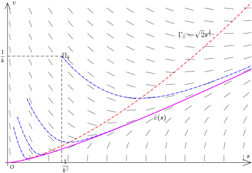
The above approximated problem is solved by the generalized phase plane analysis method. See the illustration Figure 1.

Refer to caption
Figure 1: The singular phase plane corresponding to system (2.9): the dash-dot lines correspond to solutions v~k(s)\tilde{v}_{k}(s) for different kk in the proof of Lemma 2.5, the solid line corresponds to the limit function v~(s)\tilde{v}(s).
Lemma 2.5.

For any s0>0s_{0}>0 and any 1k2<s0\frac{1}{k^{2}}<s_{0} (i.e. kk0k\geq k_{0}), the problem (2.12) admits a solution v~k(s)>0\tilde{v}_{k}(s)>0 on s(1k2,s0)s\in(\frac{1}{k^{2}},s_{0}) such that
(i)\mathrm{(i)} v~k(s)\tilde{v}_{k}(s) is monotone decreasing with respect to kk, i.e., v~k1(s)>v~k2(s)\tilde{v}_{k_{1}}(s)>\tilde{v}_{k_{2}}(s) for any k2>k1k0k_{2}>k_{1}\geq k_{0} on their joint interval (1k12,s0)(1k22,s0)=(1k12,s0)(\frac{1}{k_{1}^{2}},s_{0})\cap(\frac{1}{k_{2}^{2}},s_{0})=(\frac{1}{k_{1}^{2}},s_{0});
(ii)\mathrm{(ii)} v~k(s)\tilde{v}_{k}(s) has the following upper bound estimate

v~k(s)Γ¯k(s):={1k,s(1k2,(12k)23]2s32,s((12k)23,s0)=max{1k,2s32},s(1k2,s0);\tilde{v}_{k}(s)\leq\overline{\Gamma}_{k}(s):=\begin{cases}\displaystyle\frac{1}{k},~{}&s\in\Big{(}\frac{1}{k^{2}},(\frac{1}{\sqrt{2}k})^{\frac{2}{3}}\Big{]}\\[8.53581pt] \displaystyle\sqrt{2}s^{\frac{3}{2}},~{}&s\in\Big{(}(\frac{1}{\sqrt{2}k})^{\frac{2}{3}},s_{0}\Big{)}\end{cases}=\max\Big{\{}\frac{1}{k},\sqrt{2}s^{\frac{3}{2}}\Big{\}},\quad s\in\Big{(}\frac{1}{k^{2}},s_{0}\Big{)};

(iii)\mathrm{(iii)} v~k(s)\tilde{v}_{k}(s) has the following uniformly lower bound estimate for any μ(0,2)\mu\in(0,\sqrt{2})

v~k(s)Γμ(s):={(2μ)s32,s(0,δμ](2μ)δμ32,s(δμ,s0)=min{(2μ)s32,(2μ)δμ32},\tilde{v}_{k}(s)\geq\Gamma_{\mu}(s):=\begin{cases}\displaystyle(\sqrt{2}-\mu)s^{\frac{3}{2}},~{}&s\in(0,\delta_{\mu}]\\[8.53581pt] \displaystyle(\sqrt{2}-\mu)\delta_{\mu}^{\frac{3}{2}},~{}&s\in(\delta_{\mu},s_{0})\end{cases}=\min\left\{(\sqrt{2}-\mu)s^{\frac{3}{2}},(\sqrt{2}-\mu)\delta_{\mu}^{\frac{3}{2}}\right\},

where δμ:=μ32\delta_{\mu}:=\frac{\mu}{3\sqrt{2}}.

Proof. In the phase plane of (2.9), define an auxiliary function

Γ0(s):=2s32,s>0.\Gamma_{0}(s):=\sqrt{2}s^{\frac{3}{2}},\quad s>0.

The system (2.9) is locally uniquely solvable at any point (s,v)+×+(s,v)\in\mathbbm{R}^{+}\times\mathbbm{R}^{+} and the vector field is denoted by

Φ(s,v):=v,Ψ(s,v):=s+v2s.\Phi(s,v):=-v,\qquad\Psi(s,v):=-s+\frac{v}{\sqrt{2s}}.

There is no stationary point and no closed periodic orbit (since Φ(s,v)<0\Phi(s,v)<0 or according to Bendixson’s criterion such that div(s,v)(Φ,Ψ)=12s>0\mathrm{div}_{(s,v)}(\Phi,\Psi)=\frac{1}{\sqrt{2s}}>0) within the first quadrant, then the Poincáre-Bendixson Theorem implies that any trajectory must runs to the boundary of the first quadrant for x±x\rightarrow\pm\infty. According to the smoothness and the absence of stationary point of the vector field (Φ,Ψ)(\Phi,\Psi) within the first quadrant, we know that any two trajectories can not intersect with each other at any point (s,v)+×+(s,v)\in\mathbbm{R}^{+}\times\mathbbm{R}^{+}. The graph of Γ0\Gamma_{0} (also denoted by Γ0\Gamma_{0}) divides the first quadrant into two parts

G1:={(s,v)+×+;v>Γ0(s)},G2:={(s,v)+×+;v<Γ0(s)}.G_{1}:=\{(s,v)\in\mathbbm{R}^{+}\times\mathbbm{R}^{+};v>\Gamma_{0}(s)\},\quad G_{2}:=\{(s,v)\in\mathbbm{R}^{+}\times\mathbbm{R}^{+};v<\Gamma_{0}(s)\}.

For any point (s,v)G1(s,v)\in G_{1}, locally Φ<0\Phi<0 and Ψ>0\Psi>0, which means the trajectory runs through (s,v)(s,v) to the left-up direction if the autonomous independent variable xx grows; similarly, for any point (s,v)G2(s,v)\in G_{2}, locally Φ<0\Phi<0 and Ψ<0\Psi<0.

For any s0>0s_{0}>0 and any 1k2<s0\frac{1}{k^{2}}<s_{0} (i.e. kk0k\geq k_{0}), consider the dynamic system (2.9) with initial condition sk(xk)=1k2s_{k}(x_{k})=\frac{1}{k^{2}} and vk(xk)=1kv_{k}(x_{k})=\frac{1}{k}, where xk(0,+)x_{k}\in(0,+\infty) is a constant to be determined. The trajectory corresponding to this local solution is denoted by Πk:={(sk(x),vk(x))}\Pi_{k}:=\{(s_{k}(x),v_{k}(x))\}. Since the system (2.9) is autonomous, we will shift xkx_{k} to a suitable position in the following proof. Within the first quadrant, sx(x)=Φ(s,v)=v<0s_{x}(x)=\Phi(s,v)=-v<0, which means that s(x)s(x) is strictly decreasing with respect to xx. We can take xx as an inverse function of ss in the range of s(x)s(x) and then regard v(x)v(x) as a function of ss, this is the local solution v~k(s)\tilde{v}_{k}(s) of (2.12). The choice of xkx_{k} has no influence on the function v~k(s)\tilde{v}_{k}(s).

We only consider the trajectory Πk\Pi_{k} in the negative xx direction, that is, we consider the solution (sk(x),vk(x))(s_{k}(x),v_{k}(x)) such that x<xkx<x_{k} and xx is decreasing. Noticing that (1k2,1k)G1(\frac{1}{k^{2}},\frac{1}{k})\in G_{1} (for k2k\geq 2 without loss of generality), we see that Πk\Pi_{k} runs through (1k2,1k)(\frac{1}{k^{2}},\frac{1}{k}) in the right-down direction until it reaches some point at Γ0\Gamma_{0}. This must happen since Γ0(s)\Gamma_{0}(s) is increasing and Γ0((12k)23)=1k\Gamma_{0}((\frac{1}{\sqrt{2}k})^{\frac{2}{3}})=\frac{1}{k}. Therefore, there exists a x^k<xk\hat{x}_{k}<x_{k} such that sk(x^k)=:s^k(1k2,(12k)23)s_{k}(\hat{x}_{k})=:\hat{s}_{k}\in(\frac{1}{k^{2}},(\frac{1}{\sqrt{2}k})^{\frac{2}{3}}) and vk(x^k)=:v^kv_{k}(\hat{x}_{k})=:\hat{v}_{k}, satisfying

v^k=2s^k32(Γ0(1k2),Γ0((12k)23))=(2k3,1k).\hat{v}_{k}=\sqrt{2}\hat{s}_{k}^{\frac{3}{2}}\in\Big{(}\Gamma_{0}(\frac{1}{k^{2}}),\Gamma_{0}((\frac{1}{\sqrt{2}k})^{\frac{2}{3}})\Big{)}=\Big{(}\frac{\sqrt{2}}{k^{3}},\frac{1}{k}\Big{)}. (2.13)

Locally at the point (s^k,v^k)Γ0(\hat{s}_{k},\hat{v}_{k})\in\Gamma_{0}, Φ<0\Phi<0 and Ψ=0\Psi=0. Noticing that Γ0(s^k)=322s^k>0\Gamma_{0}^{\prime}(\hat{s}_{k})=\frac{3\sqrt{2}}{2}\sqrt{\hat{s}_{k}}>0, we find that Πk\Pi_{k} runs into G2G_{2} region as xx decreasing from x^k\hat{x}_{k}.

We assert that Πk\Pi_{k} is under Γ0\Gamma_{0} for x<x^kx<\hat{x}_{k} (i.e., v~k(s)<Γ0(s)\tilde{v}_{k}(s)<\Gamma_{0}(s) for s>s^ks>\hat{s}_{k}) and v~k(s)\tilde{v}_{k}(s) is increasing for s>s^ks>\hat{s}_{k}. We prove by contradiction and assume that there exists a s>s^ks^{*}>\hat{s}_{k} such that v~k(s)=Γ0(s)\tilde{v}_{k}(s^{*})=\Gamma_{0}(s^{*}) and v~k(s)<Γ0(s)\tilde{v}_{k}(s)<\Gamma_{0}(s) for s(s^k,s)s\in(\hat{s}_{k},s^{*}), which means there exists x<x^kx^{*}<\hat{x}_{k} such that sk(x)=ss_{k}(x^{*})=s^{*} and vk(x)=v~k(s)=Γ0(s)=:vv_{k}(x^{*})=\tilde{v}_{k}(s^{*})=\Gamma_{0}(s^{*})=:v^{*}. Then v~k(s)Γ0(s)\tilde{v}_{k}^{\prime}(s^{*})\geq\Gamma_{0}^{\prime}(s^{*}), and Γ0(s)=322s\Gamma_{0}^{\prime}(s^{*})=\frac{3\sqrt{2}}{2}\sqrt{s^{*}}, but

v~k(s)=[dvk(x)dxdsk(x)dx]x=x=sk+vk2skvk|x=x=sv12s=0\tilde{v}_{k}^{\prime}(s^{*})=\left[\frac{\frac{\mathrm{d}v_{k}(x)}{\mathrm{d}x}}{\frac{\mathrm{d}s_{k}(x)}{\mathrm{d}x}}\right]_{x=x^{*}}=\frac{-s_{k}+\frac{v_{k}}{\sqrt{2s_{k}}}}{-v_{k}}\Big{|}_{x=x^{*}}=\frac{s^{*}}{v^{*}}-\frac{1}{\sqrt{2s^{*}}}=0

at this point, which is a contradiction. Now that we have proved v~k(s)<Γ0(s)\tilde{v}_{k}(s)<\Gamma_{0}(s) for s>s^ks>\hat{s}_{k}, or equivalently, (sk(x),vk(x))G2(s_{k}(x),v_{k}(x))\in G_{2} for x<x^kx<\hat{x}_{k}. Therefore,

v~k(s)=sv~k12s>0,(s,v~k(s))G2,\tilde{v}_{k}^{\prime}(s)=\frac{s}{\tilde{v}_{k}}-\frac{1}{\sqrt{2s}}>0,\qquad(s,\tilde{v}_{k}(s))\in G_{2}, (2.14)

which shows that v~k(s)\tilde{v}_{k}(s) is increasing for s>s^ks>\hat{s}_{k}. To summarize, we proved that v~k(s)\tilde{v}_{k}(s) is decreasing for s(1k2,s^k)s\in(\frac{1}{k^{2}},\hat{s}_{k}) and increasing for s>s^ks>\hat{s}_{k}, which means v~k(s)v^k\tilde{v}_{k}(s)\geq\hat{v}_{k} with v^k>2k3\hat{v}_{k}>\frac{\sqrt{2}}{k^{3}} satisfying (2.13). Furthermore, we see that

sk(x)=Φ(sk,vk)=vk(x)=v~k(sk(x))v^k<2k3,s_{k}^{\prime}(x)=\Phi(s_{k},v_{k})=-v_{k}(x)=-\tilde{v}_{k}(s_{k}(x))\leq-\hat{v}_{k}<-\frac{\sqrt{2}}{k^{3}},

which implies that

k32s01k2s01v~k(s)ds<0-\frac{k^{3}}{\sqrt{2}}s_{0}\leq-\int_{\frac{1}{k^{2}}}^{s_{0}}\frac{1}{\tilde{v}_{k}(s)}\mathrm{d}s<0

is finite. We would shift xk=1k2s01v~k(s)dsx_{k}=\int_{\frac{1}{k^{2}}}^{s_{0}}\frac{1}{\tilde{v}_{k}(s)}\mathrm{d}s such that sk(0)=s0s_{k}(0)=s_{0}.

The above arguments imply that v~k(s)Γ¯k(s)\tilde{v}_{k}(s)\leq\overline{\Gamma}_{k}(s) for s(1k2,s0)s\in(\frac{1}{k^{2}},s_{0}). Next, we show the monotone dependence of v~k(s)\tilde{v}_{k}(s) with respect to kk. For any k2>k1k0k_{2}>k_{1}\geq k_{0}, the trajectory Πk2\Pi_{k_{2}} runs through (1k22,1k2)(\frac{1}{k_{2}^{2}},\frac{1}{k_{2}}) in the right-down direction (for xx decreasing) until it reaches some point (1k12,v)G1(\frac{1}{k_{1}^{2}},v_{*})\in G_{1} with v<1k2<1k1v_{*}<\frac{1}{k_{2}}<\frac{1}{k_{1}} or some point (s,v)(s_{*},v_{*}) on Γ0\Gamma_{0} with s(1k22,1k12]s_{*}\in(\frac{1}{k_{2}^{2}},\frac{1}{k_{1}^{2}}]. In the latter case, Πk2\Pi_{k_{2}} runs across Γ0\Gamma_{0} into G2G_{2}, and as shown by the above arguments (i.e., (2.13) and (2.14)), v~k2(s)<Γ0(s)\tilde{v}_{k_{2}}(s)<\Gamma_{0}(s) and v~k2(s)\tilde{v}_{k_{2}}(s) is increasing for s>ss>s_{*}. Therefore, v~k2(1k12)(v,Γ0(1k12))(v,1k1)\tilde{v}_{k_{2}}(\frac{1}{k_{1}^{2}})\in(v_{*},\Gamma_{0}(\frac{1}{k_{1}^{2}}))\subset(v_{*},\frac{1}{k_{1}}). In all cases, v~k2(1k12)<1k1=v~k1(1k12)\tilde{v}_{k_{2}}(\frac{1}{k_{1}^{2}})<\frac{1}{k_{1}}=\tilde{v}_{k_{1}}(\frac{1}{k_{1}^{2}}). The comparison v~k2(s)<v~k1(s)\tilde{v}_{k_{2}}(s)<\tilde{v}_{k_{1}}(s) for s>1k12s>\frac{1}{k_{1}^{2}} follows from the fact that any two trajectories cannot intersect with each other in the first quadrant.

Lastly we show the uniformly lower bound of v~k(s)\tilde{v}_{k}(s). For any μ(0,2)\mu\in(0,\sqrt{2}) and δμ:=μ32\delta_{\mu}:=\frac{\mu}{3\sqrt{2}}, we consider the special curve Γμ\Gamma_{\mu} defined by v=Γμ(s)v=\Gamma_{\mu}(s). For any point (sˇ,vˇ)Γμ(\check{s},\check{v})\in\Gamma_{\mu} with sˇ(0,δμ)\check{s}\in(0,\delta_{\mu}) and vˇ=Γμ(sˇ)\check{v}=\Gamma_{\mu}(\check{s}), the direction of vector field

Ψ(sˇ,vˇ)Φ(sˇ,vˇ)=sˇvˇ12sˇ=sˇ(2μ)sˇ3212sˇ=μ(2μ)2sˇ>μ2sˇ,\frac{\Psi(\check{s},\check{v})}{\Phi(\check{s},\check{v})}=\frac{\check{s}}{\check{v}}-\frac{1}{\sqrt{2\check{s}}}=\frac{\check{s}}{(\sqrt{2}-\mu)\check{s}^{\frac{3}{2}}}-\frac{1}{\sqrt{2\check{s}}}=\frac{\mu}{(\sqrt{2}-\mu)\sqrt{2}\sqrt{\check{s}}}>\frac{\mu}{2\sqrt{\check{s}}}, (2.15)

and the derivative of the curve Γμ\Gamma_{\mu}

Γμ(sˇ)=32(2μ)sˇ<322sˇ<μ2sˇ<Ψ(sˇ,vˇ)Φ(sˇ,vˇ)\Gamma_{\mu}^{\prime}(\check{s})=\frac{3}{2}(\sqrt{2}-\mu)\sqrt{\check{s}}<\frac{3}{2}\sqrt{2}\sqrt{\check{s}}<\frac{\mu}{2\sqrt{\check{s}}}<\frac{\Psi(\check{s},\check{v})}{\Phi(\check{s},\check{v})}

for sˇ<δμ=μ32\check{s}<\delta_{\mu}=\frac{\mu}{3\sqrt{2}}. For any point (sˇ,vˇ)Γμ(\check{s},\check{v})\in\Gamma_{\mu} with sˇδμ\check{s}\geq\delta_{\mu} and vˇ=Γμ(sˇ)=(2μ)δμ32\check{v}=\Gamma_{\mu}(\check{s})=(\sqrt{2}-\mu)\delta_{\mu}^{\frac{3}{2}}, the direction of vector field

Ψ(sˇ,vˇ)Φ(sˇ,vˇ)=sˇvˇ12sˇ>0,\frac{\Psi(\check{s},\check{v})}{\Phi(\check{s},\check{v})}=\frac{\check{s}}{\check{v}}-\frac{1}{\sqrt{2\check{s}}}>0, (2.16)

since (sˇ,vˇ)G2(\check{s},\check{v})\in G_{2} as Γμ(s)<Γ0(s)\Gamma_{\mu}(s)<\Gamma_{0}(s), and the curve Γμ\Gamma_{\mu} is horizontal. Noticing that Φ(s,v)=v<0\Phi(s,v)=-v<0, we see that any trajectory (s(x),v(x))(s(x),v(x)) runs rightwards as xx decreasing. It follows from (2.15) and (2.16) that any trajectory starting from a point (s,v)(s,v) above Γμ\Gamma_{\mu} cannot run through Γμ\Gamma_{\mu} as the independent variable xx decreasing. Therefore, v~k(s)>Γμ(s)\tilde{v}_{k}(s)>\Gamma_{\mu}(s) for s(1k2,s0)s\in(\frac{1}{k^{2}},s_{0}) since (1k2,1k)G1(\frac{1}{k^{2}},\frac{1}{k})\in G_{1} is above Γμ\Gamma_{\mu} for k2k\geq 2. The proof is completed. \hfill\Box

The solutions {v~k(s)}\{\tilde{v}_{k}(s)\} to the above approximated problem (2.12) are not defined for all s>0s>0, only on (1k2,s0)(\frac{1}{k^{2}},s_{0}). We define

v~k(s):={v~k(s),s(1k2,s0],1k,s(0,1k2],\tilde{v}_{k}^{*}(s):=\begin{cases}\tilde{v}_{k}(s),\ \ \ \ s\in\left.\left(\frac{1}{k^{2}},s_{0}\right.\right],\\[11.38109pt] \frac{1}{k},\ \ \ \ s\in\left.\left(0,\frac{1}{k^{2}}\right.\right],\end{cases}

and

v~(s)=limkv~k(s),s(0,s0).\tilde{v}(s)=\lim_{k\rightarrow\infty}\tilde{v}_{k}^{*}(s),\ \ \ \ s\in(0,s_{0}). (2.17)
Lemma 2.6.

The function v~(s)\tilde{v}(s) is well-defined in (2.17) for s(0,s0)s\in(0,s_{0}) and v~(s)\tilde{v}(s) is a solution to the singular problem (2.10). Moreover, for any μ(0,2)\mu\in(0,\sqrt{2}), let Γμ\Gamma_{\mu} be the function defined in Lemma 2.5, then Γμ(s)v~(s)2s32\Gamma_{\mu}(s)\leq\tilde{v}(s)\leq\sqrt{2}s^{\frac{3}{2}} for all s(0,s0)s\in(0,s_{0}), which means v~(s)=2s32+o(s32)\tilde{v}(s)=\sqrt{2}s^{\frac{3}{2}}+o(s^{\frac{3}{2}}) as s0+s\rightarrow 0^{+}.

Proof. For any fixed s(0,s0)s\in(0,s_{0}), v~k(s)\tilde{v}_{k}(s) is defined on (1k2,s0)(\frac{1}{k^{2}},s_{0}), which contains ss if 1k2<s\frac{1}{k^{2}}<s, i.e., k[1s]+1k\geq[\frac{1}{\sqrt{s}}]+1. According to Lemma 2.5, {v~k(s)}\{\tilde{v}_{k}(s)\} is monotone decreasing with respect to kk and is bounded. Meanwhile, {v~k(s)}\{\tilde{v}_{k}^{*}(s)\} is monotone decreasing with respect to kk and is bounded on (0,s0](0,s_{0}]. Therefore, the limit v~(s)=limkv~k(s)\tilde{v}(s)=\lim_{k\rightarrow\infty}\tilde{v}_{k}^{*}(s) exists, and satisfies Γμ(s)v~(s)2s32\Gamma_{\mu}(s)\leq\tilde{v}(s)\leq\sqrt{2}s^{\frac{3}{2}}. It is easy to check that v~(s)>0\tilde{v}(s)>0 for s(0,s0)s\in(0,s_{0}), lims0+v~(s)=0\lim_{s\rightarrow 0^{+}}\tilde{v}(s)=0, and 0s01v~(s)ds=+\int_{0}^{s_{0}}\frac{1}{\tilde{v}(s)}\mathrm{d}s=+\infty.

We show that v~(s)\tilde{v}(s) satisfies the differential equation (2.10). Locally in a neighbourhood of any s1(0,s0)s_{1}\in(0,s_{0}), say I:=(s12,s0)I:=(\frac{s_{1}}{2},s_{0}), we rewrite the differential equation (2.12) (for large kk such that 1k2<s12\frac{1}{k^{2}}<\frac{s_{1}}{2}) as

12dds(v~k)2=sv~k2s,sI.\frac{1}{2}\frac{\mathrm{d}}{\mathrm{d}s}(\tilde{v}_{k})^{2}=s-\frac{\tilde{v}_{k}}{\sqrt{2s}},\quad s\in I.

Integrating from s1s_{1} shows

12(v~k(s))212(v~k(s1))2=12s212s12s1sv~k(τ)2τdτ,sI.\frac{1}{2}(\tilde{v}_{k}(s))^{2}-\frac{1}{2}(\tilde{v}_{k}(s_{1}))^{2}=\frac{1}{2}s^{2}-\frac{1}{2}s_{1}^{2}-\int_{s_{1}}^{s}\frac{\tilde{v}_{k}(\tau)}{\sqrt{2\tau}}\mathrm{d}\tau,\quad s\in I. (2.18)

Since v~k(s)\tilde{v}_{k}(s) is monotone decreasing with respect to kk and bounded, Lebesgue’s Dominated Convergence Theorem (or Levi’s Theorem) implies that

12(v~(s))212(v~(s1))2=12s212s12s1sv~(τ)2τdτ,sI.\frac{1}{2}(\tilde{v}(s))^{2}-\frac{1}{2}(\tilde{v}(s_{1}))^{2}=\frac{1}{2}s^{2}-\frac{1}{2}s_{1}^{2}-\int_{s_{1}}^{s}\frac{\tilde{v}(\tau)}{\sqrt{2\tau}}\mathrm{d}\tau,\quad s\in I. (2.19)

Differentiating (2.19) with respect to ss near s1s_{1}, we have

v~(s)dv~(s)ds=sv~(s)2s,sI.\tilde{v}(s)\cdot\frac{\mathrm{d}\tilde{v}(s)}{\mathrm{d}s}=s-\frac{\tilde{v}(s)}{\sqrt{2s}},\quad s\in I.

Therefore, v~(s)\tilde{v}(s) is a solution to the problem (2.10). \hfill\Box

Lemma 2.7.

For s0=12u212u+2(0,16)s_{0}=\frac{1}{2}u_{-}^{2}-\frac{1}{2}u_{+}^{2}\in(0,\frac{1}{6}), let v~(s)\tilde{v}(s) for s(0,s0)s\in(0,s_{0}) be the solution to the problem (2.10) as defined in (2.17), and let s(x)s(x) and v(x)v(x) be the functions defined by (2.11) in Lemma 2.4. Then q¯(x)=s(x)\bar{q}(x)=-s(x) is a stationary solution to the problem (2.6) for the degenerate case of u+=0u_{+}=0, and has the following decay estimates

1(1s0+x22)2q¯(x)1(1s0+x2)2,x(0,+),-\frac{1}{\Big{(}\frac{1}{\sqrt{s_{0}}}+\frac{x}{2\sqrt{2}}\Big{)}^{2}}\leq\bar{q}(x)\leq-\frac{1}{\Big{(}\frac{1}{\sqrt{s_{0}}}+\frac{x}{\sqrt{2}}\Big{)}^{2}},\quad x\in(0,+\infty), (2.20)

and

22(1s0+x2)3q¯x(x)2(1s0+x22)3,x(0,+).\frac{\frac{\sqrt{2}}{2}}{\Big{(}\frac{1}{\sqrt{s_{0}}}+\frac{x}{\sqrt{2}}\Big{)}^{3}}\leq\bar{q}_{x}(x)\leq\frac{\sqrt{2}}{\Big{(}\frac{1}{\sqrt{s_{0}}}+\frac{x}{2\sqrt{2}}\Big{)}^{3}},\quad x\in(0,+\infty). (2.21)

Proof. According to Lemma 2.6, v~(s)=2s32+o(s32)\tilde{v}(s)=\sqrt{2}s^{\frac{3}{2}}+o(s^{\frac{3}{2}}) as s0+s\rightarrow 0^{+}, and Γμ(s)v~(s)2s32\Gamma_{\mu}(s)\leq\tilde{v}(s)\leq\sqrt{2}s^{\frac{3}{2}} for all s(0,s0)s\in(0,s_{0}) and μ=22\mu=\frac{\sqrt{2}}{2}, then the function s(x)s(x) defined by (2.11) satisfies (note that 0<s(x)<s00<s(x)<s_{0})

x=s0s(x)1v~(τ)dτs0s(x)12τ32dτ=2(1s(x)1s0),x(0,+),x=-\int_{s_{0}}^{s(x)}\frac{1}{\tilde{v}(\tau)}\mathrm{d}\tau\geq-\int_{s_{0}}^{s(x)}\frac{1}{\sqrt{2}\tau^{\frac{3}{2}}}\mathrm{d}\tau=\sqrt{2}\Big{(}\frac{1}{\sqrt{s(x)}}-\frac{1}{\sqrt{s_{0}}}\Big{)},\ \ \ \ x\in(0,+\infty), (2.22)

and on the other hand,

x=\displaystyle x= s0s(x)1v~(τ)dτs0s(x)1Γ22(τ)dτ=s0s(x)22τ32dτ\displaystyle-\int_{s_{0}}^{s(x)}\frac{1}{\tilde{v}(\tau)}\mathrm{d}\tau\leq-\int_{s_{0}}^{s(x)}\frac{1}{\Gamma_{\frac{\sqrt{2}}{2}}(\tau)}\mathrm{d}\tau=-\int_{s_{0}}^{s(x)}\frac{2}{\sqrt{2}\tau^{\frac{3}{2}}}\mathrm{d}\tau
=\displaystyle= 22(1s(x)1s0),x(0,+),\displaystyle 2\sqrt{2}\Big{(}\frac{1}{\sqrt{s(x)}}-\frac{1}{\sqrt{s_{0}}}\Big{)},\qquad x\in(0,+\infty), (2.23)

since Γ22(s)=(222)s32\Gamma_{\frac{\sqrt{2}}{2}}(s)=(\sqrt{2}-\frac{\sqrt{2}}{2})s^{\frac{3}{2}} for s(0,δ22)s\in(0,\delta_{\frac{\sqrt{2}}{2}}) and δ22=2/232=16>s0\delta_{\frac{\sqrt{2}}{2}}=\frac{\sqrt{2}/2}{3\sqrt{2}}=\frac{1}{6}>s_{0}. Combining the above estimates (2.22) and (2.23) implies

1(1s0+x2)2s(x)1(1s0+x22)2,x(0,+).\frac{1}{\Big{(}\frac{1}{\sqrt{s_{0}}}+\frac{x}{\sqrt{2}}\Big{)}^{2}}\leq s(x)\leq\frac{1}{\Big{(}\frac{1}{\sqrt{s_{0}}}+\frac{x}{2\sqrt{2}}\Big{)}^{2}},\quad x\in(0,+\infty). (2.24)

Since s(x)s(x) is a solution to the problem (2.9), we have

sx(x)=v(x)=v~(s(x))[2s32(x),Γ22(s(x))],x(0,+).s_{x}(x)=-v(x)=-\tilde{v}(s(x))\in[-\sqrt{2}s^{\frac{3}{2}}(x),-\Gamma_{\frac{\sqrt{2}}{2}}(s(x))],\quad x\in(0,+\infty).

That is,

sx(x)22s32(x)22(1s0+x2)3,s_{x}(x)\leq-\frac{\sqrt{2}}{2}s^{\frac{3}{2}}(x)\leq-\frac{\frac{\sqrt{2}}{2}}{\Big{(}\frac{1}{\sqrt{s_{0}}}+\frac{x}{\sqrt{2}}\Big{)}^{3}},

and

sx(x)2s32(x)2(1s0+x22)3,s_{x}(x)\geq-\sqrt{2}s^{\frac{3}{2}}(x)\geq-\frac{\sqrt{2}}{\Big{(}\frac{1}{\sqrt{s_{0}}}+\frac{x}{2\sqrt{2}}\Big{)}^{3}},

for x(0,+)x\in(0,+\infty). \hfill\Box

Remark 2.1.

The restriction of s0<16s_{0}<\frac{1}{6} is not essential for the existence and the decay estimates of the stationary solution in Lemma 2.7. For general s016s_{0}\geq\frac{1}{6}, we can modify the estimate (2.23) such that

s0s(x)1Γ22(τ)dτ={16s(x)22τ32dτs0161Γ22(16)dτ,if s(x)<16,s0s(x)1Γ22(16)dτ,if s(x)>16.-\int_{s_{0}}^{s(x)}\frac{1}{\Gamma_{\frac{\sqrt{2}}{2}}(\tau)}\mathrm{d}\tau=\begin{cases}\displaystyle-\int_{\frac{1}{6}}^{s(x)}\frac{2}{\sqrt{2}\tau^{\frac{3}{2}}}\mathrm{d}\tau-\int_{s_{0}}^{\frac{1}{6}}\frac{1}{\Gamma_{\frac{\sqrt{2}}{2}}(\frac{1}{6})}\mathrm{d}\tau,~{}&\text{if~{}}s(x)<\frac{1}{6},\\[17.07164pt] \displaystyle-\int_{s_{0}}^{s(x)}\frac{1}{\Gamma_{\frac{\sqrt{2}}{2}}(\frac{1}{6})}\mathrm{d}\tau,~{}&\text{if~{}}s(x)>\frac{1}{6}.\end{cases}

The decay estimates follow similarly. Here we take s0<16s_{0}<\frac{1}{6} for the sake of the simplicity of the expressions. This remark is valid for all the estimates in this subsection, hence we only present the precise estimates for small s0s_{0}.

The asymptotic behavior v~(s)=2s32+o(s32)\tilde{v}(s)=\sqrt{2}s^{\frac{3}{2}}+o(s^{\frac{3}{2}}) as s0+s\rightarrow 0^{+} implies the decay estimates of q¯(x)\bar{q}(x) and q¯x(x)\bar{q}_{x}(x). In order to derive decay estimates of higher order derivatives, we expand v~(s)\tilde{v}(s) to higher order. Define sequences {ck}\{c_{k}\} and {ak}\{a_{k}\} as following

c1=1,ck=i+j=k(2j+1)cicj,k2,c_{1}=1,\quad c_{k}=\sum_{i+j=k}(2j+1)c_{i}\cdot c_{j},\quad\forall k\geq 2, (2.25)

and

ak=(1)k+12ck,k1.a_{k}=(-1)^{k+1}\sqrt{2}c_{k},\quad\forall k\geq 1. (2.26)

For example, a1=2a_{1}=\sqrt{2}, a2=32a_{2}=-3\sqrt{2}, a3=242a_{3}=24\sqrt{2}, a4=2852a_{4}=-285\sqrt{2}, a5=42842a_{5}=4284\sqrt{2}. The formal series

i=1ais2i+12\sum_{i=1}^{\infty}a_{i}s^{\frac{2i+1}{2}}

is not convergent at any point s>0s>0, and then the infinite series expansion method cannot be applied. However, the finite series expansion still gives the local behavior of the solution v~(s)\tilde{v}(s), which leads to the precise decay estimates of the higher order derivatives of q¯(x)\bar{q}(x) and u¯(x)\bar{u}(x).

Lemma 2.8.

For any k+k\in\mathbbm{N}^{+}, there holds

v~(s)=i=1kais2i+12+o(s2k+12),s0+.\tilde{v}(s)=\sum_{i=1}^{k}a_{i}s^{\frac{2i+1}{2}}+o(s^{\frac{2k+1}{2}}),\quad s\rightarrow 0^{+}.

Specifically, for odd k+k\in\mathbbm{N}^{+}, there exist δk>0\delta_{k}>0 and Mk>0M_{k}>0 such that

i=1kais2i+12Mks2k+32v~(s)i=1kais2i+12,s(0,δk);\sum_{i=1}^{k}a_{i}s^{\frac{2i+1}{2}}-M_{k}s^{\frac{2k+3}{2}}\leq\tilde{v}(s)\leq\sum_{i=1}^{k}a_{i}s^{\frac{2i+1}{2}},\quad s\in(0,\delta_{k});

while for even k+k\in\mathbbm{N}^{+}, there exist δk>0\delta_{k}>0 and Mk>0M_{k}>0 such that

i=1kais2i+12v~(s)i=1kais2i+12+Mks2k+32,s(0,δk).\sum_{i=1}^{k}a_{i}s^{\frac{2i+1}{2}}\leq\tilde{v}(s)\leq\sum_{i=1}^{k}a_{i}s^{\frac{2i+1}{2}}+M_{k}s^{\frac{2k+3}{2}},\quad s\in(0,\delta_{k}).

Proof. We prove the cases k=2k=2 and k=3k=3. Other cases follow similarly. For k=2k=2, let β(s):=2s32v~(s)\beta(s):=\sqrt{2}s^{\frac{3}{2}}-\tilde{v}(s), i.e., v~(s)=2s32β(s)\tilde{v}(s)=\sqrt{2}s^{\frac{3}{2}}-\beta(s). The function v~(s)=2s32+o(s32)\tilde{v}(s)=\sqrt{2}s^{\frac{3}{2}}+o(s^{\frac{3}{2}}) as s0+s\rightarrow 0^{+} satisfies the differential equation (2.10), and then β(s)\beta(s) satisfies

dv~ds=322sdβ(s)ds=sv~12s=s2s32β(s)12s.\displaystyle\frac{\mathrm{d}\tilde{v}}{\mathrm{d}s}=\frac{3}{2}\sqrt{2s}-\frac{\mathrm{d}\beta(s)}{\mathrm{d}s}=\frac{s}{\tilde{v}}-\frac{1}{\sqrt{2s}}=\frac{s}{\sqrt{2}s^{\frac{3}{2}}-\beta(s)}-\frac{1}{\sqrt{2s}}.

That is,

dβ(s)ds=322s+12ss2s32β(s)=32s52(1+3s)β(s)2s22sβ(s).\frac{\mathrm{d}\beta(s)}{\mathrm{d}s}=\frac{3}{2}\sqrt{2s}+\frac{1}{\sqrt{2s}}-\frac{s}{\sqrt{2}s^{\frac{3}{2}}-\beta(s)}=\frac{3\sqrt{2}s^{\frac{5}{2}}-(1+3s)\cdot\beta(s)}{2s^{2}-\sqrt{2s}\cdot\beta(s)}. (2.27)

We analyze the phase plane (s,β)(s,\beta) corresponding to the singular differential equation (2.27) in a similar way as we solve the problem (2.10).

Consider two special curves in the phase plane of (s,β)(s,\beta)

Γ(s):=32s52,Γ(s):=32s52M2s72,s(0,δ2),\Gamma^{*}(s):=3\sqrt{2}s^{\frac{5}{2}},\quad\Gamma_{*}(s):=3\sqrt{2}s^{\frac{5}{2}}-M_{2}s^{\frac{7}{2}},\quad s\in(0,\delta_{2}), (2.28)

where M2>0M_{2}>0 and δ2>0\delta_{2}>0 are constants to be determined.

We use the same symbol Γ\Gamma^{*} (or Γ\Gamma_{*}) to denote the curve as well as the function. At any point (s^,β^)Γ(\hat{s},\hat{\beta})\in\Gamma^{*} (i.e., β^=32s^52\hat{\beta}=3\sqrt{2}\hat{s}^{\frac{5}{2}}), there holds

Γ(s^)=1522s^32>0>32s^52(1+3s^)β^2s^22s^β^=dβ(s)ds|s=s^,β=β^.\Gamma^{*}{}^{\prime}(\hat{s})=\frac{15}{2}\sqrt{2}\hat{s}^{\frac{3}{2}}>0>\frac{3\sqrt{2}\hat{s}^{\frac{5}{2}}-(1+3\hat{s})\cdot\hat{\beta}}{2\hat{s}^{2}-\sqrt{2\hat{s}}\cdot\hat{\beta}}=\frac{\mathrm{d}\beta(s)}{\mathrm{d}s}\Big{|}_{s=\hat{s},\beta=\hat{\beta}}. (2.29)

Meanwhile, at any point (s^,β^)Γ(\hat{s},\hat{\beta})\in\Gamma_{*} (i.e., β^=32s^52M2s^72\hat{\beta}=3\sqrt{2}\hat{s}^{\frac{5}{2}}-M_{2}\hat{s}^{\frac{7}{2}}), we have

Γ(s^)=1522s^3272M2s^52<32s^52(1+3s^)β^2s^22s^β^=dβ(s)ds|s=s^,β=β^,\Gamma_{*}^{\prime}(\hat{s})=\frac{15}{2}\sqrt{2}\hat{s}^{\frac{3}{2}}-\frac{7}{2}M_{2}\hat{s}^{\frac{5}{2}}<\frac{3\sqrt{2}\hat{s}^{\frac{5}{2}}-(1+3\hat{s})\cdot\hat{\beta}}{2\hat{s}^{2}-\sqrt{2\hat{s}}\cdot\hat{\beta}}=\frac{\mathrm{d}\beta(s)}{\mathrm{d}s}\Big{|}_{s=\hat{s},\beta=\hat{\beta}}, (2.30)

which is equivalent to

1522s^3272M2s^52<(M292)s^72+3M2s^922s^26s^3+M22s^4.\frac{15}{2}\sqrt{2}\hat{s}^{\frac{3}{2}}-\frac{7}{2}M_{2}\hat{s}^{\frac{5}{2}}<\frac{(M_{2}-9\sqrt{2})\hat{s}^{\frac{7}{2}}+3M_{2}\hat{s}^{\frac{9}{2}}}{2\hat{s}^{2}-6\hat{s}^{3}+M_{2}\sqrt{2}\hat{s}^{4}}.

It suffices to take M2=242M_{2}=24\sqrt{2} and δ2=18\delta_{2}=\frac{1}{8}. The analysis of the trajectories according to inequalities (2.29) and (2.30) show that

32s52M2s72β(s)32s52,s(0,δ2).3\sqrt{2}s^{\frac{5}{2}}-M_{2}s^{\frac{7}{2}}\leq\beta(s)\leq 3\sqrt{2}s^{\frac{5}{2}},\quad s\in(0,\delta_{2}).

Therefore,

v~(s)=2s32β(s){2s3232s52,2s3232s52+M2s72,s(0,δ2).\tilde{v}(s)=\sqrt{2}s^{\frac{3}{2}}-\beta(s)~{}\begin{cases}\geq\sqrt{2}s^{\frac{3}{2}}-3\sqrt{2}s^{\frac{5}{2}},\\[5.69054pt] \leq\sqrt{2}s^{\frac{3}{2}}-3\sqrt{2}s^{\frac{5}{2}}+M_{2}s^{\frac{7}{2}},\end{cases}\qquad s\in(0,\delta_{2}). (2.31)

Next, we consider the case of k=3k=3. Let α(s):=v~(s)2s32+32s52\alpha(s):=\tilde{v}(s)-\sqrt{2}s^{\frac{3}{2}}+3\sqrt{2}s^{\frac{5}{2}}, i.e., v~(s)=2s3232s52+α(s)\tilde{v}(s)=\sqrt{2}s^{\frac{3}{2}}-3\sqrt{2}s^{\frac{5}{2}}+\alpha(s). According to the differential equation (2.10) of v~(s)\tilde{v}(s), we see that α(s)\alpha(s) satisfies

dv~ds=322s1522s32+dα(s)ds=sv~12s=s2s3232s52+α(s)12s.\displaystyle\frac{\mathrm{d}\tilde{v}}{\mathrm{d}s}=\frac{3}{2}\sqrt{2s}-\frac{15}{2}\sqrt{2}s^{\frac{3}{2}}+\frac{\mathrm{d}\alpha(s)}{\mathrm{d}s}=\frac{s}{\tilde{v}}-\frac{1}{\sqrt{2s}}=\frac{s}{\sqrt{2}s^{\frac{3}{2}}-3\sqrt{2}s^{\frac{5}{2}}+\alpha(s)}-\frac{1}{\sqrt{2s}}.

It is equivalent to

dα(s)ds=\displaystyle\frac{\mathrm{d}\alpha(s)}{\mathrm{d}s}= s2s3232s52+α(s)12s322s+1522s32\displaystyle\frac{s}{\sqrt{2}s^{\frac{3}{2}}-3\sqrt{2}s^{\frac{5}{2}}+\alpha(s)}-\frac{1}{\sqrt{2s}}-\frac{3}{2}\sqrt{2s}+\frac{15}{2}\sqrt{2}s^{\frac{3}{2}}
=\displaystyle= (13s+15s2)α(s)+(242s72452s92)2s26s3+2sα(s).\displaystyle\frac{(-1-3s+15s^{2})\cdot\alpha(s)+(24\sqrt{2}s^{\frac{7}{2}}-45\sqrt{2}s^{\frac{9}{2}})}{2s^{2}-6s^{3}+\sqrt{2s}\cdot\alpha(s)}. (2.32)

The two special curves that are used to control the trajectories in the phase plane (s,α)(s,\alpha) corresponding to (2.32) are

Γ¯(s):=242s72,Γ¯(s):=242s72M3s92,s(0,δ3),\bar{\Gamma}^{*}(s):=24\sqrt{2}s^{\frac{7}{2}},\quad\bar{\Gamma}_{*}(s):=24\sqrt{2}s^{\frac{7}{2}}-M_{3}s^{\frac{9}{2}},\quad s\in(0,\delta_{3}), (2.33)

with M3=2852M_{3}=285\sqrt{2} and δ3=min{18,15,77285}=18\delta_{3}=\min\{\frac{1}{8},\frac{1}{5},\frac{77}{285}\}=\frac{1}{8}. Here we omit the details showing that at any point (s^,α^)Γ¯(\hat{s},\hat{\alpha})\in\bar{\Gamma}^{*}

Γ¯(s^)>0>dα(s)ds|s=s^,α=α^,s(0,δ3),\bar{\Gamma}^{*}{}^{\prime}(\hat{s})>0>\frac{\mathrm{d}\alpha(s)}{\mathrm{d}s}\Big{|}_{s=\hat{s},\alpha=\hat{\alpha}},\quad s\in(0,\delta_{3}),

and at any point (s^,α^)Γ¯(\hat{s},\hat{\alpha})\in\bar{\Gamma}_{*}

Γ¯(s^)<dα(s)ds|s=s^,α=α^,s(0,δ3).\bar{\Gamma}_{*}^{\prime}(\hat{s})<\frac{\mathrm{d}\alpha(s)}{\mathrm{d}s}\Big{|}_{s=\hat{s},\alpha=\hat{\alpha}},\quad s\in(0,\delta_{3}).

It follows that

242s72M3s92α(s)242s72,s(0,δ3),24\sqrt{2}s^{\frac{7}{2}}-M_{3}s^{\frac{9}{2}}\leq\alpha(s)\leq 24\sqrt{2}s^{\frac{7}{2}},\quad s\in(0,\delta_{3}),

and further

v~(s)=2s3232s52+α(s){2s3232s52+242s72M3s92,2s3232s52+242s72,s(0,δ3).\tilde{v}(s)=\sqrt{2}s^{\frac{3}{2}}-3\sqrt{2}s^{\frac{5}{2}}+\alpha(s)~{}\begin{cases}\geq\sqrt{2}s^{\frac{3}{2}}-3\sqrt{2}s^{\frac{5}{2}}+24\sqrt{2}s^{\frac{7}{2}}-M_{3}s^{\frac{9}{2}},\\[5.69054pt] \leq\sqrt{2}s^{\frac{3}{2}}-3\sqrt{2}s^{\frac{5}{2}}+24\sqrt{2}s^{\frac{7}{2}},\end{cases}\ \ \ s\in(0,\delta_{3}). (2.34)

Generally, we can take Mk=|ak+1|M_{k}=|a_{k+1}|. The proof is completed. \hfill\Box

We now show the decay estimates of higher order derivatives of q¯(x)\bar{q}(x).

Lemma 2.9.

For s0<18s_{0}<\frac{1}{8}, let q¯(x)\bar{q}(x) be the stationary solution proved in Lemma 2.7. Then

3(1s0+x22)4q¯xx(x)0,x(0,+),-\frac{3}{\Big{(}\frac{1}{\sqrt{s_{0}}}+\frac{x}{2\sqrt{2}}\Big{)}^{4}}\leq\bar{q}_{xx}(x)\leq 0,\quad x\in(0,+\infty), (2.35)

and

|q¯xxx(x)|62(1s0+x22)5+C(1s0+x22)7,x(0,+),|\bar{q}_{xxx}(x)|\leq\frac{6\sqrt{2}}{\Big{(}\frac{1}{\sqrt{s_{0}}}+\frac{x}{2\sqrt{2}}\Big{)}^{5}}+\frac{C}{\Big{(}\frac{1}{\sqrt{s_{0}}}+\frac{x}{2\sqrt{2}}\Big{)}^{7}},\quad x\in(0,+\infty), (2.36)

for some positive constant C>0C>0. For s0<δ4s_{0}<\delta_{4} (δ4\delta_{4} is the positive constant in Lemma 2.8), there holds

|q¯xxxx(x)|222(1s0+x22)6+C(1s0+x22)8,|\bar{q}_{xxxx}(x)|\leq\frac{222}{\Big{(}\frac{1}{\sqrt{s_{0}}}+\frac{x}{2\sqrt{2}}\Big{)}^{6}}+\frac{C}{\Big{(}\frac{1}{\sqrt{s_{0}}}+\frac{x}{2\sqrt{2}}\Big{)}^{8}}, (2.37)

for some positive constant C>0C>0.

Proof. According to the dynamic system (2.9),

sx(x)=v(x),vx(x)=s(x)+v(x)2s(x).s_{x}(x)=-v(x),\qquad v_{x}(x)=-s(x)+\frac{v(x)}{\sqrt{2s(x)}}.

We have

sxx(x)=vx(x)=s(x)v(x)2s(x)=s(x)v~(s(x))2s(x).\displaystyle s_{xx}(x)=-v_{x}(x)=s(x)-\frac{v(x)}{\sqrt{2s(x)}}=s(x)-\frac{\tilde{v}(s(x))}{\sqrt{2s(x)}}.

Using the expansion (2.31) in Lemma 2.8 and the decay estimate (2.24) in Lemma 2.7, we deduce

sxx(x)s(x)2s32(x)32s52(x)2s(x)=3s2(x)3(1s0+x22)4,s_{xx}(x)\leq s(x)-\frac{\sqrt{2}s^{\frac{3}{2}}(x)-3\sqrt{2}s^{\frac{5}{2}}(x)}{\sqrt{2s(x)}}=3s^{2}(x)\leq\frac{3}{\Big{(}\frac{1}{\sqrt{s_{0}}}+\frac{x}{2\sqrt{2}}\Big{)}^{4}},

and

sxx(x)\displaystyle s_{xx}(x)\geq s(x)2s32(x)32s52(x)+242s72(x)2s(x)\displaystyle s(x)-\frac{\sqrt{2}s^{\frac{3}{2}}(x)-3\sqrt{2}s^{\frac{5}{2}}(x)+24\sqrt{2}s^{\frac{7}{2}}(x)}{\sqrt{2s(x)}}
\displaystyle\geq 3s2(x)24s3(x)max{3(1s0+x2)424(1s0+x22)6,0}.\displaystyle 3s^{2}(x)-24s^{3}(x)\geq\max\left\{\frac{3}{\Big{(}\frac{1}{\sqrt{s_{0}}}+\frac{x}{\sqrt{2}}\Big{)}^{4}}-\frac{24}{\Big{(}\frac{1}{\sqrt{s_{0}}}+\frac{x}{2\sqrt{2}}\Big{)}^{6}},0\right\}.

Similarly, we have

sxxx(x)=\displaystyle s_{xxx}(x)= vxx(x)=sx(x)vx(x)2s(x)+v(x)22s32(x)(v(x))\displaystyle-v_{xx}(x)=s_{x}(x)-\frac{v_{x}(x)}{\sqrt{2s(x)}}+\frac{v(x)}{2\sqrt{2}s^{\frac{3}{2}}(x)}\cdot(-v(x))
=\displaystyle= v(x)s(x)+v(x)2s(x)2s(x)v2(x)22s32(x)\displaystyle-v(x)-\frac{-s(x)+\frac{v(x)}{\sqrt{2s(x)}}}{\sqrt{2s(x)}}-\frac{v^{2}(x)}{2\sqrt{2}s^{\frac{3}{2}}(x)} (2.38)
=\displaystyle= v~(s(x))+s(x)2v~(s(x))2s(x)(v~(s(x)))222s32(x).\displaystyle-\tilde{v}(s(x))+\frac{\sqrt{s(x)}}{\sqrt{2}}-\frac{\tilde{v}(s(x))}{2s(x)}-\frac{(\tilde{v}(s(x)))^{2}}{2\sqrt{2}s^{\frac{3}{2}}(x)}.

Utilizing the expansion (2.34) in Lemma 2.8, we deduce

sxxx(x)\displaystyle s_{xxx}(x)\leq (2s3232s52+242s722852s92)+s2\displaystyle-(\sqrt{2}s^{\frac{3}{2}}-3\sqrt{2}s^{\frac{5}{2}}+24\sqrt{2}s^{\frac{7}{2}}-285\sqrt{2}s^{\frac{9}{2}})+\frac{\sqrt{s}}{\sqrt{2}}
2s3232s52+242s722852s922s\displaystyle-\frac{\sqrt{2}s^{\frac{3}{2}}-3\sqrt{2}s^{\frac{5}{2}}+24\sqrt{2}s^{\frac{7}{2}}-285\sqrt{2}s^{\frac{9}{2}}}{2s}
(2s3232s52+242s722852s92)222s32\displaystyle-\frac{(\sqrt{2}s^{\frac{3}{2}}-3\sqrt{2}s^{\frac{5}{2}}+24\sqrt{2}s^{\frac{7}{2}}-285\sqrt{2}s^{\frac{9}{2}})^{2}}{2\sqrt{2}s^{\frac{3}{2}}}
\displaystyle\leq 62s52(x)+Cs72(x),\displaystyle-6\sqrt{2}s^{\frac{5}{2}}(x)+Cs^{\frac{7}{2}}(x),

and

sxxx(x)\displaystyle s_{xxx}(x)\geq (2s3232s52+242s72)+s2\displaystyle-(\sqrt{2}s^{\frac{3}{2}}-3\sqrt{2}s^{\frac{5}{2}}+24\sqrt{2}s^{\frac{7}{2}})+\frac{\sqrt{s}}{\sqrt{2}}
2s3232s52+242s722s(2s3232s52+242s72)222s32\displaystyle-\frac{\sqrt{2}s^{\frac{3}{2}}-3\sqrt{2}s^{\frac{5}{2}}+24\sqrt{2}s^{\frac{7}{2}}}{2s}-\frac{(\sqrt{2}s^{\frac{3}{2}}-3\sqrt{2}s^{\frac{5}{2}}+24\sqrt{2}s^{\frac{7}{2}})^{2}}{2\sqrt{2}s^{\frac{3}{2}}}
\displaystyle\geq 62s52(x)Cs72(x),\displaystyle-6\sqrt{2}s^{\frac{5}{2}}(x)-Cs^{\frac{7}{2}}(x),

where C>0C>0 is a generic positive constant. Therefore,

|sxxx(x)|62s52(x)+Cs72(x)62(1s0+x22)5+C(1s0+x22)7.|s_{xxx}(x)|\leq 6\sqrt{2}s^{\frac{5}{2}}(x)+Cs^{\frac{7}{2}}(x)\leq\frac{6\sqrt{2}}{\Big{(}\frac{1}{\sqrt{s_{0}}}+\frac{x}{2\sqrt{2}}\Big{)}^{5}}+\frac{C}{\Big{(}\frac{1}{\sqrt{s_{0}}}+\frac{x}{2\sqrt{2}}\Big{)}^{7}}.

We now show the estimates of sxxxx(x)s_{xxxx}(x). According to (2.38),

sxxxx(x)=\displaystyle s_{xxxx}(x)= vx(x)+(s(x)2)x(v(x)2s(x))x(v2(x)22s32(x))x\displaystyle-v_{x}(x)+\Big{(}\frac{\sqrt{s(x)}}{\sqrt{2}}\Big{)}_{x}-\Big{(}\frac{v(x)}{2s(x)}\Big{)}_{x}-\Big{(}\frac{v^{2}(x)}{2\sqrt{2}s^{\frac{3}{2}}(x)}\Big{)}_{x}
=\displaystyle= (s(x)+v(x)2s(x))v(x)22s(x)s(x)+v(x)2s(x)2s(x)v2(x)2s2(x)\displaystyle-\Big{(}-s(x)+\frac{v(x)}{\sqrt{2s(x)}}\Big{)}-\frac{v(x)}{2\sqrt{2s(x)}}-\frac{-s(x)+\frac{v(x)}{\sqrt{2s(x)}}}{2s(x)}-\frac{v^{2}(x)}{2s^{2}(x)}
2v(x)(s(x)+v(x)2s(x))22s32(x)32v3(x)22s52(x).\displaystyle-\frac{2v(x)\cdot(-s(x)+\frac{v(x)}{\sqrt{2s(x)}})}{2\sqrt{2}s^{\frac{3}{2}}(x)}-\frac{\frac{3}{2}v^{3}(x)}{2\sqrt{2}s^{\frac{5}{2}}(x)}. (2.39)

Substituting v(x)=v~(s(x))v(x)=\tilde{v}(s(x)) and the expansion of v~(s)\tilde{v}(s) for k=4k=4 in Lemma 2.8 such that

v~(s){2s3232s52+242s722852s92,2s3232s52+242s722852s92+42842s112,s(0,δ4),\tilde{v}(s)~{}\begin{cases}\geq\sqrt{2}s^{\frac{3}{2}}-3\sqrt{2}s^{\frac{5}{2}}+24\sqrt{2}s^{\frac{7}{2}}-285\sqrt{2}s^{\frac{9}{2}},\\[5.69054pt] \leq\sqrt{2}s^{\frac{3}{2}}-3\sqrt{2}s^{\frac{5}{2}}+24\sqrt{2}s^{\frac{7}{2}}-285\sqrt{2}s^{\frac{9}{2}}+4284\sqrt{2}s^{\frac{11}{2}},\end{cases}\quad s\in(0,\delta_{4}),

into (2.39) implies that

|sxxxx(x)|222s3(x)+Cs4(x)222(1s0+x22)6+C(1s0+x22)8,|s_{xxxx}(x)|\leq 222s^{3}(x)+Cs^{4}(x)\leq\frac{222}{\Big{(}\frac{1}{\sqrt{s_{0}}}+\frac{x}{2\sqrt{2}}\Big{)}^{6}}+\frac{C}{\Big{(}\frac{1}{\sqrt{s_{0}}}+\frac{x}{2\sqrt{2}}\Big{)}^{8}},

for some positive constant C>0C>0. \hfill\Box

Lemma 2.10.

For s0=12u212u+2=12u2=12δ2<min{18,δ4}s_{0}=\frac{1}{2}u_{-}^{2}-\frac{1}{2}u_{+}^{2}=\frac{1}{2}u_{-}^{2}=\frac{1}{2}\delta^{2}<\min\{\frac{1}{8},\delta_{4}\}, let q¯(x)\bar{q}(x) be the stationary solution proved in Lemma 2.7 and let u¯(x):=2q¯(x)=2s(x)\bar{u}(x):=-\sqrt{-2\bar{q}(x)}=-\sqrt{2s(x)}. Then we have

C1δ1+δxu¯(x)C2δ1+δx,\displaystyle\frac{C_{1}\delta}{1+\delta x}\leq-\bar{u}(x)\leq\frac{C_{2}\delta}{1+\delta x},\qquad C1δ2(1+δx)2u¯x(x)C2δ2(1+δx)2,\displaystyle\frac{C_{1}\delta^{2}}{(1+\delta x)^{2}}\leq\bar{u}_{x}(x)\leq\frac{C_{2}\delta^{2}}{(1+\delta x)^{2}},
|xku¯(x)|C2δk+1(1+δx)k+1,\displaystyle\Big{|}\partial^{k}_{x}\bar{u}(x)\Big{|}\leq\frac{C_{2}\delta^{k+1}}{(1+\delta x)^{k+1}},\qquad |u¯xx2(x)u¯x(x)|C2δ4(1+δx)4,\displaystyle\Big{|}\frac{\bar{u}_{xx}^{2}(x)}{\bar{u}_{x}(x)}\Big{|}\leq\frac{C_{2}\delta^{4}}{(1+\delta x)^{4}},
|u¯xxx2(x)u¯x(x)|C2δ6(1+δx)6,|u¯xxx(x)u¯x(x)|\displaystyle\Big{|}\frac{\bar{u}_{xxx}^{2}(x)}{\bar{u}_{x}(x)}\Big{|}\leq\frac{C_{2}\delta^{6}}{(1+\delta x)^{6}},\qquad\Big{|}\frac{\bar{u}_{xxx}(x)}{\bar{u}_{x}(x)}\Big{|}\leq C2δ2(1+δx)2,|u¯xxxx(x)u¯x(x)|C2δ3(1+δx)3,\displaystyle\frac{C_{2}\delta^{2}}{(1+\delta x)^{2}},\qquad\Big{|}\frac{\bar{u}_{xxxx}(x)}{\bar{u}_{x}(x)}\Big{|}\leq\frac{C_{2}\delta^{3}}{(1+\delta x)^{3}},

for k=1,2,3,4k=1,2,3,4 and some positive constants C1C_{1}, C2C_{2}.

Proof. The lower and upper bounds of q¯(x)\bar{q}(x) and q¯x(x)\bar{q}_{x}(x) in (2.20) and (2.21) in Lemma 2.7 show that

u¯(x)=2q¯(x){21s0+x2,21s0+x22,x(0,+),\bar{u}(x)=-\sqrt{-2\bar{q}(x)}~{}\begin{cases}\displaystyle\leq-\frac{\sqrt{2}}{\frac{1}{\sqrt{s_{0}}}+\frac{x}{\sqrt{2}}},\\[17.07164pt] \displaystyle\geq-\frac{\sqrt{2}}{\frac{1}{\sqrt{s_{0}}}+\frac{x}{2\sqrt{2}}},\end{cases}\quad x\in(0,+\infty),

and

u¯x(x)=q¯x2q¯{1s0+x2(1s0+x22)32(1s0+x22)2,1s0+x222(1s0+x2)314(1s0+x2)2,x(0,+).\bar{u}_{x}(x)=\frac{\bar{q}_{x}}{\sqrt{-2\bar{q}}}~{}\begin{cases}\displaystyle\leq\frac{\frac{1}{\sqrt{s_{0}}}+\frac{x}{\sqrt{2}}}{\Big{(}\frac{1}{\sqrt{s_{0}}}+\frac{x}{2\sqrt{2}}\Big{)}^{3}}\leq\frac{2}{\Big{(}\frac{1}{\sqrt{s_{0}}}+\frac{x}{2\sqrt{2}}\Big{)}^{2}},\\[22.76219pt] \displaystyle\geq\frac{\frac{1}{\sqrt{s_{0}}}+\frac{x}{2\sqrt{2}}}{2\Big{(}\frac{1}{\sqrt{s_{0}}}+\frac{x}{\sqrt{2}}\Big{)}^{3}}\geq\frac{1}{4\Big{(}\frac{1}{\sqrt{s_{0}}}+\frac{x}{\sqrt{2}}\Big{)}^{2}},\end{cases}\quad x\in(0,+\infty).

Utilizing the higher order estimates (2.35), (2.36) and (2.37) in Lemma 2.9, we have

|u¯xx(x)|=\displaystyle|\bar{u}_{xx}(x)|= |q¯xx(x)2q¯(x)+(q¯x(x))2(2q¯(x))32|3(1s0+x2)2(1s0+x22)4+(1s0+x2)32(1s0+x22)6\displaystyle\left|\frac{\bar{q}_{xx}(x)}{\sqrt{-2\bar{q}(x)}}+\frac{(\bar{q}_{x}(x))^{2}}{(-2\bar{q}(x))^{\frac{3}{2}}}\right|\leq\frac{3(\frac{1}{\sqrt{s_{0}}}+\frac{x}{\sqrt{2}})}{\sqrt{2}\Big{(}\frac{1}{\sqrt{s_{0}}}+\frac{x}{2\sqrt{2}}\Big{)}^{4}}+\frac{\Big{(}\frac{1}{\sqrt{s_{0}}}+\frac{x}{\sqrt{2}}\Big{)}^{3}}{\sqrt{2}\Big{(}\frac{1}{\sqrt{s_{0}}}+\frac{x}{2\sqrt{2}}\Big{)}^{6}}
\displaystyle\leq 72(1s0+x22)3,\displaystyle\frac{7\sqrt{2}}{\Big{(}\frac{1}{\sqrt{s_{0}}}+\frac{x}{2\sqrt{2}}\Big{)}^{3}},

and

|u¯xxx(x)|=|q¯xxx2q¯+3q¯xq¯xx(2q¯)32+3(q¯x)3(2q¯)52|C(1s0+x22)4,|\bar{u}_{xxx}(x)|=\left|\frac{\bar{q}_{xxx}}{\sqrt{-2\bar{q}}}+\frac{3\bar{q}_{x}\bar{q}_{xx}}{(-2\bar{q})^{\frac{3}{2}}}+\frac{3(\bar{q}_{x})^{3}}{(-2\bar{q})^{\frac{5}{2}}}\right|\leq\frac{C}{\Big{(}\frac{1}{\sqrt{s_{0}}}+\frac{x}{2\sqrt{2}}\Big{)}^{4}},
|u¯xxxx(x)|=|q¯xxxx2q¯+4q¯xq¯xxx+3(q¯xx)2(2q¯)32+18(q¯x)2q¯xx(2q¯)52+15(q¯x)4(2q¯)72|C(1s0+x22)5,|\bar{u}_{xxxx}(x)|=\left|\frac{\bar{q}_{xxxx}}{\sqrt{-2\bar{q}}}+\frac{4\bar{q}_{x}\bar{q}_{xxx}+3(\bar{q}_{xx})^{2}}{(-2\bar{q})^{\frac{3}{2}}}+\frac{18(\bar{q}_{x})^{2}\bar{q}_{xx}}{(-2\bar{q})^{\frac{5}{2}}}+\frac{15(\bar{q}_{x})^{4}}{(-2\bar{q})^{\frac{7}{2}}}\right|\leq\frac{C}{\Big{(}\frac{1}{\sqrt{s_{0}}}+\frac{x}{2\sqrt{2}}\Big{)}^{5}},

where C>0C>0 is a generic positive constant. Moreover,

|u¯xxxu¯x|C(1s0+x22)2,|u¯xxxxu¯x|C(1s0+x22)3,\left|\frac{\bar{u}_{xxx}}{\bar{u}_{x}}\right|\leq\frac{C}{\Big{(}\frac{1}{\sqrt{s_{0}}}+\frac{x}{2\sqrt{2}}\Big{)}^{2}},\qquad\left|\frac{\bar{u}_{xxxx}}{\bar{u}_{x}}\right|\leq\frac{C}{\Big{(}\frac{1}{\sqrt{s_{0}}}+\frac{x}{2\sqrt{2}}\Big{)}^{3}},

and

|u¯xxx2u¯x|C(1s0+x22)6,|u¯xx2u¯x|C(1s0+x22)4.\left|\frac{\bar{u}_{xxx}^{2}}{\bar{u}_{x}}\right|\leq\frac{C}{\Big{(}\frac{1}{\sqrt{s_{0}}}+\frac{x}{2\sqrt{2}}\Big{)}^{6}},\qquad\left|\frac{\bar{u}_{xx}^{2}}{\bar{u}_{x}}\right|\leq\frac{C}{\Big{(}\frac{1}{\sqrt{s_{0}}}+\frac{x}{2\sqrt{2}}\Big{)}^{4}}.

The proof is completed. \hfill\Box

Proof of Lemma 2.3. The degenerate case (2): u<u+=0u_{-}<u_{+}=0 is proved through a singular phase plane analysis method according to Lemma 2.7 and Lemma 2.10.

Next we show that this method is applicable to the case (1) u<u+<0u_{-}<u_{+}<0. Instead of (2.9), we have a non-degenerate dynamical system (2.8) for the case of u+<0u_{+}<0. We sketch the main lines of the proof.

(1) For any s0:=12u212u+2>0s_{0}:=\frac{1}{2}u_{-}^{2}-\frac{1}{2}u_{+}^{2}>0, if v~(s)\tilde{v}(s) solves the following equation

{dv~ds=sv~1u+2+2s,s(0,s0),v~(s)>0fors(0,s0),lims0+v~(s)=0,0s01v~(s)ds=+,\begin{cases}\displaystyle\frac{\mathrm{d}\tilde{v}}{\mathrm{d}s}=\frac{s}{\tilde{v}}-\frac{1}{\sqrt{u_{+}^{2}+2s}},\quad s\in(0,s_{0}),\\[17.07164pt] \displaystyle\tilde{v}(s)>0\mathrm{~{}for~{}}s\in(0,s_{0}),\quad\lim_{s\rightarrow 0^{+}}\tilde{v}(s)=0,\quad\int_{0}^{s_{0}}\frac{1}{\tilde{v}(s)}\mathrm{d}s=+\infty,\end{cases} (2.40)

then the function s(x)s(x) defined by

x=s0s(x)1v~(τ)dτ,x(0,+)x=-\int_{s_{0}}^{s(x)}\frac{1}{\tilde{v}(\tau)}\mathrm{d}\tau,\qquad x\in(0,+\infty) (2.41)

is a solution of (2.8) with v(x):=v~(s(x))>0v(x):=\tilde{v}(s(x))>0.

(2) Consider the approximated problem

{dv~kds=sv~k1u+2+2s,s(0,s0),v~k(s)>0fors(0,s0),v~k(0)=1k.\begin{cases}\displaystyle\frac{\mathrm{d}\tilde{v}_{k}}{\mathrm{d}s}=\frac{s}{\tilde{v}_{k}}-\frac{1}{\sqrt{u_{+}^{2}+2s}},\quad s\in(0,s_{0}),\\[17.07164pt] \displaystyle\tilde{v}_{k}(s)>0\mathrm{~{}for~{}}s\in(0,s_{0}),\quad\tilde{v}_{k}(0)=\frac{1}{k}.\end{cases} (2.42)

For any s0>0s_{0}>0, the problem (2.42) admits a solution v~k(s)>0\tilde{v}_{k}(s)>0 on s(0,s0)s\in(0,s_{0}) such that
(i) v~k(s)\tilde{v}_{k}(s) is monotone decreasing with respect to kk, i.e., v~k1(s)>v~k2(s)\tilde{v}_{k_{1}}(s)>\tilde{v}_{k_{2}}(s) for any k2>k1k_{2}>k_{1} on (0,s0)(0,s_{0});
(ii) v~k(s)\tilde{v}_{k}(s) has the following upper bound estimate

v~k(s)Γ¯k(s):=max{1k,su+2+2s},s(0,s0);\tilde{v}_{k}(s)\leq\overline{\Gamma}_{k}(s):=\max\Big{\{}\frac{1}{k},s\cdot\sqrt{u_{+}^{2}+2s}\Big{\}},\quad s\in(0,s_{0});

(iii) v~k(s)\tilde{v}_{k}(s) has the following uniformly lower bound estimate

v~k(s)λ0s,s(0,s0),\tilde{v}_{k}(s)\geq\lambda_{0}s,\quad s\in(0,s_{0}),

where λ0:=1+4|u+|212|u+|\lambda_{0}:=\frac{\sqrt{1+4|u_{+}|^{2}}-1}{2|u_{+}|}.

(3) The limit function

v~(s):=limkv~k(s),s(0,s0)\tilde{v}(s):=\lim_{k\rightarrow\infty}\tilde{v}_{k}(s),\quad s\in(0,s_{0})

is well-defined and v~(s)\tilde{v}(s) is a solution to the problem (2.40). Moreover,

λ0sv~(s)λ0s+bs2,s(0,s0),\lambda_{0}s\leq\tilde{v}(s)\leq\lambda_{0}s+bs^{2},\quad s\in(0,s_{0}), (2.43)

where λ0:=1+4|u+|212|u+|\lambda_{0}:=\frac{\sqrt{1+4|u_{+}|^{2}}-1}{2|u_{+}|} is the positive root of λ0=1λ01|u+|\lambda_{0}=\frac{1}{\lambda_{0}}-\frac{1}{|u_{+}|} and b=12|u+|3b=\frac{1}{2|u_{+}|^{3}}.

The asymptotic expansion (2.43) plays an essential role in the analysis of asymptotic decay behavior of the stationary solution, thus we present the following proof. In the phase plane (s,v)(s,v), at any point (s^,v^)(\hat{s},\hat{v}) on the curve v^=Γ(s^):=λ0s^\hat{v}=\Gamma_{*}(\hat{s}):=\lambda_{0}\hat{s}, we have

Γ(s^)=λ0=1λ01|u+|<s^v^1u+2+2s^=dv~ds|(s^,v^),\Gamma_{*}^{\prime}(\hat{s})=\lambda_{0}=\frac{1}{\lambda_{0}}-\frac{1}{|u_{+}|}<\frac{\hat{s}}{\hat{v}}-\frac{1}{\sqrt{u_{+}^{2}+2\hat{s}}}=\left.\frac{\mathrm{d}\tilde{v}}{\mathrm{d}s}\right|_{(\hat{s},\hat{v})},

which means the trajectory lies above Γ\Gamma_{*}. At any point (s^,v^)(\hat{s},\hat{v}) on the curve v^=Γ(s^):=λ0s^+bs^2\hat{v}=\Gamma^{*}(\hat{s}):=\lambda_{0}\hat{s}+b\hat{s}^{2}, we have

Γ(s^)=λ0+2bs^>s^v^1u+2+2s^=dv~ds|(s^,v^),\Gamma^{*}{}^{\prime}(\hat{s})=\lambda_{0}+2b\hat{s}>\frac{\hat{s}}{\hat{v}}-\frac{1}{\sqrt{u_{+}^{2}+2\hat{s}}}=\left.\frac{\mathrm{d}\tilde{v}}{\mathrm{d}s}\right|_{(\hat{s},\hat{v})},

since the following auxiliary function

F(s^):=λ0+2bs^1λ0+bs^+1u+2+2s^,s(0,s0)F(\hat{s}):=\lambda_{0}+2b\hat{s}-\frac{1}{\lambda_{0}+b\hat{s}}+\frac{1}{\sqrt{u_{+}^{2}+2\hat{s}}},\quad s\in(0,s_{0})

is monotonically increasing as F(s^)=2b+b(λ0+bs^)21(|u+|2+2s^)32>0F^{\prime}(\hat{s})=2b+\frac{b}{(\lambda_{0}+b\hat{s})^{2}}-\frac{1}{(|u_{+}|^{2}+2\hat{s})^{\frac{3}{2}}}>0 for b=12|u+|3b=\frac{1}{2|u_{+}|^{3}}. This shows the trajectory lies between Γ\Gamma_{*} and Γ\Gamma^{*}.

(4) Finally we show the asymptotic behavior of the stationary solution. According to the definition of s(x)s(x) and q¯(x)\bar{q}(x) in (2.41) and the asymptotic expansion (2.43), we have

x=s0s(x)1v~(τ)dτs(x)s01λ0τdτ=1λ0ln(s0s(x)),x(0,+),\displaystyle x=-\int_{s_{0}}^{s(x)}\frac{1}{\tilde{v}(\tau)}\mathrm{d}\tau\leq\int_{s(x)}^{s_{0}}\frac{1}{\lambda_{0}\tau}\mathrm{d}\tau=\frac{1}{\lambda_{0}}\ln\Big{(}\frac{s_{0}}{s(x)}\Big{)},\quad x\in(0,+\infty),

which implies

s(x)s0eλ0x,q¯(x)q¯eλ0x.s(x)\leq s_{0}\mathrm{e}^{-\lambda_{0}x},\quad\bar{q}(x)\geq\bar{q}_{-}\mathrm{e}^{-\lambda_{0}x}.

On the other hand,

x=s0s(x)1v~(τ)dτs(x)s01λ0τ+bτ2dτ=1λ0ln(τ1+bλ0τ)|s(x)s0,x(0,+).\displaystyle x=-\int_{s_{0}}^{s(x)}\frac{1}{\tilde{v}(\tau)}\mathrm{d}\tau\geq\int_{s(x)}^{s_{0}}\frac{1}{\lambda_{0}\tau+b\tau^{2}}\mathrm{d}\tau=\left.\frac{1}{\lambda_{0}}\ln\left(\frac{\tau}{1+\frac{b}{\lambda_{0}}\tau}\right)\right|_{s(x)}^{s_{0}},\qquad x\in(0,+\infty).

That is,

s(x)s01+bλ0s0eλ0x1bλ0s01+bλ0s0eλ0xs01+bλ0s0eλ0x,s(x)\geq\frac{\frac{s_{0}}{1+\frac{b}{\lambda_{0}}s_{0}}\cdot\mathrm{e}^{-\lambda_{0}x}}{1-\frac{b}{\lambda_{0}}\cdot\frac{s_{0}}{1+\frac{b}{\lambda_{0}}s_{0}}\cdot\mathrm{e}^{-\lambda_{0}x}}\geq\frac{s_{0}}{1+\frac{b}{\lambda_{0}}s_{0}}\cdot\mathrm{e}^{-\lambda_{0}x},

which shows

q¯(x)q¯1bλ0q¯eλ0x.\bar{q}(x)\leq\frac{\bar{q}_{-}}{1-\frac{b}{\lambda_{0}}\bar{q}_{-}}\cdot\mathrm{e}^{-\lambda_{0}x}.

The decay estimates of q¯x(x)\bar{q}_{x}(x) and other higher order derivatives follow similarly, which are all exponentially decaying, since

sx(x)=v(x)=v~(s(x)),s_{x}(x)=-v(x)=-\tilde{v}(s(x)),

and

sxx(x)=vx(x)=s(x)v(x)u+2+2s(s)=s(x)v~(s(x))u+2+2s(s),s_{xx}(x)=-v_{x}(x)=s(x)-\frac{v(x)}{\sqrt{u_{+}^{2}+2s(s)}}=s(x)-\frac{\tilde{v}(s(x))}{\sqrt{u_{+}^{2}+2s(s)}},

and according to the asymptotic expansion (2.43). The proof is completed. \hfill\Box

2.3 Preliminary Lemmas

In order to show the asymptotic behavior of heat flux q(x,t)q(x,t) which satisfies an elliptic problem, we prove the following optimal Gagliardo-Nirenberg-Sobolev inequality. This inequality without optimal constant is known as a special case of Gagliardo-Nirenberg-Sobolev inequality. Here we present a primary proof based on fundamental calculus.

Lemma 2.11 (Optimal Gagliardo-Nirenberg-Sobolev inequality).

For any function u(x)L()u(x)\in L^{\infty}(\mathbbm{R}) with uxxL()u_{xx}\in L^{\infty}(\mathbbm{R}), there holds

uxL()2uL()12uxxL()12,\|u_{x}\|_{L^{\infty}(\mathbbm{R})}\leq\sqrt{2}\ \|u\|_{L^{\infty}(\mathbbm{R})}^{\frac{1}{2}}\cdot\|u_{xx}\|_{L^{\infty}(\mathbbm{R})}^{\frac{1}{2}}, (2.44)

and the constant 2\sqrt{2} is optimal. Moreover, for any function u(x)L(+)u(x)\in L^{\infty}(\mathbbm{R}_{+}) with uxxL(+)u_{xx}\in L^{\infty}(\mathbbm{R}_{+}), there holds

uxL(+)2uL(+)12uxxL(+)12,\|u_{x}\|_{L^{\infty}(\mathbbm{R}_{+})}\leq 2\ \|u\|_{L^{\infty}(\mathbbm{R}_{+})}^{\frac{1}{2}}\cdot\|u_{xx}\|_{L^{\infty}(\mathbbm{R}_{+})}^{\frac{1}{2}}, (2.45)

and the constant 22 is optimal. For multi-dimensional case,

|u|L(n)2uL(n)12|D2u|L(n)12,uW2,(n),\||\nabla u|\|_{L^{\infty}(\mathbbm{R}^{n})}\leq\sqrt{2}\ \|u\|_{L^{\infty}(\mathbbm{R}^{n})}^{\frac{1}{2}}\cdot\||D^{2}u|\|_{L^{\infty}(\mathbbm{R}^{n})}^{\frac{1}{2}},\qquad\forall u\in W^{2,\infty}(\mathbbm{R}^{n}), (2.46)

and

|u|L(+n)2uL(+n)12|D2u|L(+n)12,uW2,(+n),\||\nabla u|\|_{L^{\infty}(\mathbbm{R}_{+}^{n})}\leq 2\ \|u\|_{L^{\infty}(\mathbbm{R}_{+}^{n})}^{\frac{1}{2}}\cdot\||D^{2}u|\|_{L^{\infty}(\mathbbm{R}_{+}^{n})}^{\frac{1}{2}},\qquad\forall u\in W^{2,\infty}(\mathbbm{R}_{+}^{n}), (2.47)

and the constants 2\sqrt{2} and 22 are optimal, where |u||\nabla u| is the modulus of a vector u\nabla u and |D2u||D^{2}u| is the spectral norm of a matrix D2uD^{2}u such that |D2u|:=suppn;|p|=1pT(D2u)p|D^{2}u|:=\sup_{p\in\mathbbm{R}^{n};|p|=1}p^{\mathrm{T}}(D^{2}u)p.

Proof. We prove that the inequality (2.44) holds for any smooth function uC2()W2,()u\in C^{2}(\mathbbm{R})\cap W^{2,\infty}(\mathbbm{R}) and the constant is optimal for uW2,()u\in W^{2,\infty}(\mathbbm{R}) with weak derivatives. Then utilizing an approximation approach, we see that (2.44) holds for uW2,()u\in W^{2,\infty}(\mathbbm{R}) with the same optimal constant.

The inequality (2.44) is trivial if uL()=0\|u\|_{L^{\infty}(\mathbbm{R})}=0 or uxxL()=0\|u_{xx}\|_{L^{\infty}(\mathbbm{R})}=0, since in the latter case u(x)=c1x+c2u(x)=c_{1}x+c_{2} and c1=0c_{1}=0 according to uL()u\in L^{\infty}(\mathbbm{R}). With the observation that the inequality (2.44) is invariant under the scaling u~(x):=λu(μx)\tilde{u}(x):=\lambda u(\mu x) for any non-zero λ\lambda and μ\mu, we only need to prove that uxL()1\|u_{x}\|_{L^{\infty}(\mathbbm{R})}\leq 1 under the condition uL()=12\|u\|_{L^{\infty}(\mathbbm{R})}=\frac{1}{2} and uxxL()=1\|u_{xx}\|_{L^{\infty}(\mathbbm{R})}=1, and further uxL()1\|u_{x}\|_{L^{\infty}(\mathbbm{R})}\leq 1 is optimal. In other words, we show that if ux(x0)=1u_{x}(x_{0})=1 for some x0x_{0}\in\mathbbm{R} and uxxL()1\|u_{xx}\|_{L^{\infty}(\mathbbm{R})}\leq 1 then uL()12\|u\|_{L^{\infty}(\mathbbm{R})}\geq\frac{1}{2} and 12\frac{1}{2} is optimal.

According to Taylor expansion near x0x_{0} for uC2()W2,()u\in C^{2}(\mathbbm{R})\cap W^{2,\infty}(\mathbbm{R}), we know that

u(x0+1)\displaystyle u(x_{0}+1) u(x0)+ux(x0)1+12uxx(ξ1)12u(x0)+112,\displaystyle\geq u(x_{0})+u_{x}(x_{0})\cdot 1+\frac{1}{2}u_{xx}(\xi_{1})\cdot 1^{2}\geq u(x_{0})+1-\frac{1}{2},
u(x01)\displaystyle u(x_{0}-1) u(x0)+ux(x0)(1)+12uxx(ξ2)(1)2u(x0)1+12,\displaystyle\leq u(x_{0})+u_{x}(x_{0})\cdot(-1)+\frac{1}{2}u_{xx}(\xi_{2})\cdot(-1)^{2}\leq u(x_{0})-1+\frac{1}{2},

with some ξ1(x0,x0+1)\xi_{1}\in(x_{0},x_{0}+1) and ξ2(x01,x0)\xi_{2}\in(x_{0}-1,x_{0}). Therefore,

u(x0+1)u(x01)1,u(x_{0}+1)-u(x_{0}-1)\geq 1,

and then uL()12\|u\|_{L^{\infty}(\mathbbm{R})}\geq\frac{1}{2}. The constant is optimal for the following u^1W2,()\hat{u}_{1}\in W^{2,\infty}(\mathbbm{R})

u^1(x):={,x(112x),x[0,2),(x2)(212x),x[2,4),\hat{u}_{1}(x):=\begin{cases}\cdots,\\[2.84526pt] x(1-\frac{1}{2}x),\ \ \ \ x\in[0,2),\\[2.84526pt] (x-2)(2-\frac{1}{2}x),\ \ \ \ x\in[2,4),\\[2.84526pt] \cdots\end{cases} (2.48)

which is defined by extension as a 44-periodic function. We can verify that u^1(x)\hat{u}_{1}(x) satisfies the following differential equation

u^1xx=signu1={1,u1>0,1,u1<0.-\hat{u}_{1xx}=\mathrm{sign}u_{1}=\begin{cases}1,\ \ \ \ u_{1}>0,\\[2.84526pt] -1,\ \ \ \ u_{1}<0.\end{cases}

The inequality (2.45) for uW2,(+)u\in W^{2,\infty}(\mathbbm{R}_{+}) is proved by extension

u~(x):={u(x),x0,2u(0)u(x),x<0,\tilde{u}(x):=\begin{cases}u(x),\ \ \ \ x\geq 0,\\[5.69054pt] 2u(0)-u(-x),\ \ \ \ x<0,\end{cases}

such that u~xL()=uxL(+)\|\tilde{u}_{x}\|_{L^{\infty}(\mathbbm{R})}=\|u_{x}\|_{L^{\infty}(\mathbbm{R}_{+})}, u~xxL()=uxxL(+)\|\tilde{u}_{xx}\|_{L^{\infty}(\mathbbm{R})}=\|u_{xx}\|_{L^{\infty}(\mathbbm{R}_{+})}, and

osc(u;+)osc(u~;)2osc(u;+)4uL(+).\mathrm{osc}(u;\mathbbm{R}_{+})\leq\mathrm{osc}(\tilde{u};\mathbbm{R})\leq 2\mathrm{osc}(u;\mathbbm{R}_{+})\leq 4\|u\|_{L^{\infty}(\mathbbm{R}_{+})}.

Here osc(f;D):=supx,yD|f(x)f(y)|\mathrm{osc}(f;D):=\sup_{x,y\in D}|f(x)-f(y)| is the oscillation of a given function ff and DD is its domain of definition. Furthermore, applying (2.44) (according to the proof, we can replace u~L()\|\tilde{u}\|_{L^{\infty}(\mathbbm{R})} by 12osc(u~;)\frac{1}{2}\mathrm{osc}(\tilde{u};\mathbbm{R}))

uxL(+)=u~xL()(osc(u~;))12u~xxL()122uL()12uxxL()12.\|u_{x}\|_{L^{\infty}(\mathbbm{R}_{+})}=\|\tilde{u}_{x}\|_{L^{\infty}(\mathbbm{R})}\leq(\mathrm{osc}(\tilde{u};\mathbbm{R}))^{\frac{1}{2}}\cdot\|\tilde{u}_{xx}\|_{L^{\infty}(\mathbbm{R})}^{\frac{1}{2}}\leq 2\ \|u\|_{L^{\infty}(\mathbbm{R})}^{\frac{1}{2}}\cdot\|u_{xx}\|_{L^{\infty}(\mathbbm{R})}^{\frac{1}{2}}.

The constant 22 is optimal for the following u^2(x)\hat{u}_{2}(x)

u^2(x):={x(112x)14,x[0,1),14,x[1,+),\hat{u}_{2}(x):=\begin{cases}x(1-\frac{1}{2}x)-\frac{1}{4},\ \ \ \ x\in[0,1),\\[5.69054pt] \frac{1}{4},\ \ \ \ x\in[1,+\infty),\end{cases} (2.49)

such that u^2L(+)=14\|\hat{u}_{2}\|_{L^{\infty}(\mathbbm{R}_{+})}=\frac{1}{4}, u^2xL(+)=1\|\hat{u}_{2x}\|_{L^{\infty}(\mathbbm{R}_{+})}=1 and u^2xxL(+)=1\|\hat{u}_{2xx}\|_{L^{\infty}(\mathbbm{R}_{+})}=1.

For the multi-dimensional case, we note that the inequality (2.46) is invariant under the scaling u~(x):=λu(μx)\tilde{u}(x):=\lambda u(\mu x) for any non-zero λ\lambda and μ\mu, and is also invariant under the rotation of coordinates. Therefore, for any function uC2(n)W2,(n)u\in C^{2}(\mathbbm{R}^{n})\cap W^{2,\infty}(\mathbbm{R}^{n}), if |u(x0)|=1|\nabla u(x_{0})|=1 for some x0nx_{0}\in\mathbbm{R}^{n} and |D2u(x)|1|D^{2}u(x)|\leq 1 for all xnx\in\mathbbm{R}^{n}, then Taylor expansion along the direction ±p:=±u(x0)\pm p:=\pm\nabla u(x_{0}) shows that

u(x0+u(x0))\displaystyle u(x_{0}+\nabla u(x_{0})) u(x0)+u(x0)u(x0)+12(u(x0))T(D2u(ξ1))(u(x0))u(x0)+112,\displaystyle\geq u(x_{0})+\nabla u(x_{0})\cdot\nabla u(x_{0})+\frac{1}{2}(\nabla u(x_{0}))^{\mathrm{T}}(D^{2}u(\xi_{1}))(\nabla u(x_{0}))\geq u(x_{0})+1-\frac{1}{2},
u(x0u(x0))\displaystyle u(x_{0}-\nabla u(x_{0})) u(x0)u(x0)u(x0)+12(u(x0))T(D2u(ξ2))(u(x0))u(x0)1+12,\displaystyle\leq u(x_{0})-\nabla u(x_{0})\cdot\nabla u(x_{0})+\frac{1}{2}(-\nabla u(x_{0}))^{\mathrm{T}}(D^{2}u(\xi_{2}))(-\nabla u(x_{0}))\leq u(x_{0})-1+\frac{1}{2},

for some ξ1=x0+θ1u(x0)\xi_{1}=x_{0}+\theta_{1}\nabla u(x_{0}) and ξ2=x0θ2u(x0)\xi_{2}=x_{0}-\theta_{2}\nabla u(x_{0}) with θ1,θ2(0,1)\theta_{1},\theta_{2}\in(0,1). The rest of the proof follows similarly. \hfill\Box

Remark 2.2.

Lemma 2.11 can be seen as a special case of Gagliardo-Nirenberg-Sobolev inequality with the optimal constant and without the restriction of decay at infinity such that lim|x|+u(x)=0\lim_{|x|\rightarrow+\infty}u(x)=0.

Lemma 2.12.

Assume that fL(+)f\in L^{\infty}(\mathbbm{R}_{+}), gg\in\mathbbm{R}, and uW2,(+)u\in W^{2,\infty}(\mathbbm{R}_{+}) solves the following elliptic problem

{uxx+u=f(x),x>0,ux(0)=g,\begin{cases}-u_{xx}+u=f(x),\quad&x>0,\\[2.84526pt] u_{x}(0)=g,\end{cases} (2.50)

then

uL(+)fL(+)+|g|,uxL(+)fL(+)+|g|,uxxL(+)2fL(+)+|g|,\|u\|_{L^{\infty}(\mathbbm{R}_{+})}\leq\|f\|_{L^{\infty}(\mathbbm{R}_{+})}+|g|,\quad\|u_{x}\|_{L^{\infty}(\mathbbm{R}_{+})}\leq\|f\|_{L^{\infty}(\mathbbm{R}_{+})}+|g|,\quad\|u_{xx}\|_{L^{\infty}(\mathbbm{R}_{+})}\leq 2\|f\|_{L^{\infty}(\mathbbm{R}_{+})}+|g|, (2.51)

and all the above coefficients are optimal.

Proof. Let v(x):=u(x)+gexv(x):=u(x)+g\mathrm{e}^{-x}. Then vW2,(+)v\in W^{2,\infty}(\mathbbm{R}_{+}) satisfies

{vxx+v=f(x),x>0,vx(0)=0.\begin{cases}-v_{xx}+v=f(x),\quad&x>0,\\[2.84526pt] v_{x}(0)=0.\end{cases} (2.52)

Maximum principle shows that vL(+)fL(+)\|v\|_{L^{\infty}(\mathbbm{R}_{+})}\leq\|f\|_{L^{\infty}(\mathbbm{R}_{+})} and then uL(+)fL(+)+|g|\|u\|_{L^{\infty}(\mathbbm{R}_{+})}\leq\|f\|_{L^{\infty}(\mathbbm{R}_{+})}+|g|. Further, according to the equation (2.50) we have uxxL(+)2fL(+)+|g|\|u_{xx}\|_{L^{\infty}(\mathbbm{R}_{+})}\leq 2\|f\|_{L^{\infty}(\mathbbm{R}_{+})}+|g|. According to Lemma 2.11, we see that

uxL(+)2uL(+)12uxxL(+)122(fL(+)+|g|)12(2fL(+)+|g|)12.\|u_{x}\|_{L^{\infty}(\mathbbm{R}_{+})}\leq 2\ \|u\|_{L^{\infty}(\mathbbm{R}_{+})}^{\frac{1}{2}}\cdot\|u_{xx}\|_{L^{\infty}(\mathbbm{R}_{+})}^{\frac{1}{2}}\leq 2\ (\|f\|_{L^{\infty}(\mathbbm{R}_{+})}+|g|)^{\frac{1}{2}}\cdot(2\|f\|_{L^{\infty}(\mathbbm{R}_{+})}+|g|)^{\frac{1}{2}}.

Here the Gagliardo-Nirenberg-Sobolev inequality in Lemma 2.11 is optimal for all uW2,(+)u\in W^{2,\infty}(\mathbbm{R}_{+}) but not for the solutions of elliptic problem (2.50). In order to show optimal estimates, we extend the functions ff and vv in (2.52) such that

f~(x):={f(x),x0,f(x),x<0, and v~(x):={v(x),x0,v(x),x<0.\tilde{f}(x):=\begin{cases}f(x),\ \ \ \ x\geq 0,\\ f(-x),\ \ \ \ x<0,\end{cases}\quad\text{~{}and~{}}\quad\tilde{v}(x):=\begin{cases}v(x),\ \ \ \ x\geq 0,\\ v(-x),\ \ \ \ x<0.\end{cases}

Then v~\tilde{v} can be solved as

v~(x)=12e|xy|f~(y)dy=120+(e|xy|+e|x+y|)f(y)dy,x.\tilde{v}(x)=\frac{1}{2}\int_{\mathbbm{R}}\mathrm{e}^{-|x-y|}\tilde{f}(y)\mathrm{d}y=\frac{1}{2}\int_{0}^{+\infty}\left(\mathrm{e}^{-|x-y|}+\mathrm{e}^{-|x+y|}\right)f(y)\mathrm{d}y,\quad x\in\mathbbm{R}.

Therefore, for x0x\geq 0,

u(x)\displaystyle u(x) =120+(e|xy|+e|x+y|)f(y)dygex,\displaystyle=\frac{1}{2}\int_{0}^{+\infty}\left(\mathrm{e}^{-|x-y|}+\mathrm{e}^{-|x+y|}\right)f(y)\mathrm{d}y-g\mathrm{e}^{-x}, (2.53)
ux(x)\displaystyle u_{x}(x) =120+(e|xy|(sign(xy))+e|x+y|(1))f(y)dy+gex,\displaystyle=\frac{1}{2}\int_{0}^{+\infty}\left(\mathrm{e}^{-|x-y|}(-\mathrm{sign(x-y)})+\mathrm{e}^{-|x+y|}(-1)\right)f(y)\mathrm{d}y+g\mathrm{e}^{-x}, (2.54)

and

uxx(x)=120+(e|xy|+e|x+y|)f(y)dygexf(x).u_{xx}(x)=\frac{1}{2}\int_{0}^{+\infty}\left(\mathrm{e}^{-|x-y|}+\mathrm{e}^{-|x+y|}\right)f(y)\mathrm{d}y-g\mathrm{e}^{-x}-f(x). (2.55)

The above expressions show that the estimates (2.51) are valid.

Now we show that all these coefficients are optimal. The special case of f(x)0f(x)\equiv 0, g=1g=-1 and u(x)=exu(x)=\mathrm{e}^{-x} implies that the coefficients of |g||g| in (2.51) are optimal. The case of g=0g=0, f(x)1f(x)\equiv 1 and u(x)1u(x)\equiv 1 shows that the coefficient of fL(+)\|f\|_{L^{\infty}(\mathbbm{R}_{+})} in the estimate of uL(+)\|u\|_{L^{\infty}(\mathbbm{R}_{+})} is optimal. For any large x0>0x_{0}>0, we set f(x)=sign(xx0)f(x)=\mathrm{sign}(x-x_{0}) and g=0g=0, then (2.54) implies

ux(x0)=\displaystyle u_{x}(x_{0})= 120x0(e|x0y|+e|x0+y|)dy+12x0+(e|x0y|e|x0+y|)dy\displaystyle\frac{1}{2}\int_{0}^{x_{0}}\left(\mathrm{e}^{-|x_{0}-y|}+\mathrm{e}^{-|x_{0}+y|}\right)\mathrm{d}y+\frac{1}{2}\int_{x_{0}}^{+\infty}\left(\mathrm{e}^{-|x_{0}-y|}-\mathrm{e}^{-|x_{0}+y|}\right)\mathrm{d}y
=\displaystyle= 1202x0eydy+120+eydy122x0+eydy\displaystyle\frac{1}{2}\int_{0}^{2x_{0}}\mathrm{e}^{-y}\mathrm{d}y+\frac{1}{2}\int_{0}^{+\infty}\mathrm{e}^{-y}\mathrm{d}y-\frac{1}{2}\int_{2x_{0}}^{+\infty}\mathrm{e}^{-y}\mathrm{d}y
=\displaystyle= 12x0+eydy1,as x0+,\displaystyle 1-\int_{2x_{0}}^{+\infty}\mathrm{e}^{-y}\mathrm{d}y\rightarrow 1,\quad\text{as~{}}x_{0}\rightarrow+\infty,

which shows that the coefficient of fL(+)\|f\|_{L^{\infty}(\mathbbm{R}_{+})} in the estimate of uxL(+)\|u_{x}\|_{L^{\infty}(\mathbbm{R}_{+})} is optimal. Lastly, for g=0g=0, small ε>0\varepsilon>0, and f(x)=sign(xε)f(x)=\mathrm{sign}(x-\varepsilon), according to (2.55), we have

uxx(0)\displaystyle u_{xx}(0) =0+eyf(y)dyf(0)\displaystyle=\int_{0}^{+\infty}\mathrm{e}^{-y}f(y)\mathrm{d}y-f(0)
=0εey(1)dy+ε+ey(+1)dy(1)\displaystyle=\int_{0}^{\varepsilon}\mathrm{e}^{-y}(-1)\mathrm{d}y+\int_{\varepsilon}^{+\infty}\mathrm{e}^{-y}(+1)\mathrm{d}y-(-1)
=220εeydy2,as ε0,\displaystyle=2-2\int_{0}^{\varepsilon}\mathrm{e}^{-y}\mathrm{d}y\rightarrow 2,\quad\text{as~{}}~{}~{}\varepsilon\rightarrow 0,

and the coefficient of fL(+)\|f\|_{L^{\infty}(\mathbbm{R}_{+})} in the estimate of uxxL(+)\|u_{xx}\|_{L^{\infty}(\mathbbm{R}_{+})} is optimal. \hfill\Box

2.4 Main Theorems

We state our main results for the cases: u<u+0u_{-}<u_{+}\leq 0, 0u<u+0\leq u_{-}<u_{+} and u<0<u+u_{-}<0<u_{+}, that the initial-boundary value problem (1.1)-(1.3) admits a unique global solution and it converges to the stationary solution, the rarefaction wave and the superposition of the nonlinear waves, respectively, as tt\to\infty.

Theorem 2.13 (In the case of 0<u<u+0<u_{-}<u_{+}).

Suppose that the boundary condition and far field states satisfy 0<u<u+0<u_{-}<u_{+}, the initial data u0u_{0} satisfies u0u~0RH2(+)u_{0}-\tilde{u}_{0}^{R}\in H^{2}(\mathbbm{R}_{+}), where u~0R\tilde{u}_{0}^{R} is defined in (2.2). Also assume that δ=|uu+|\delta=|u_{-}-u_{+}| is sufficiently small. Then there is a positive constant ϵ0\epsilon_{0} such that if u0u~0R2+δϵ0\|u_{0}-\tilde{u}_{0}^{R}\|_{2}+\delta\leq\epsilon_{0}, the problem (1.1)-(1.3) admits a unique solution (u(x,t),q(x,t))(u(x,t),q(x,t)), which satisfies

uuRC0([0,);H2)C1([0,);H1),\displaystyle u-u^{R}\in C^{0}([0,\infty);H^{2})\cap C^{1}([0,\infty);H^{1}),
q+xuRC0([0,);H3)L2(0,;H3),\displaystyle q+\partial_{x}u^{R}\in C^{0}([0,\infty);H^{3})\cap L^{2}(0,\infty;H^{3}),

and the asymptotic behavior

supx+|xk(u(x,t)uR(x))|0ast,k=0,1,supx+|xk(q(x,t)+xuR(x))|0ast,k=0,1,2.\begin{split}&\sup_{x\in\mathbbm{R}_{+}}\left|\partial_{x}^{k}\left(u(x,t)-u^{R}(x)\right)\right|\rightarrow 0\ \ \text{as}\ \ t\rightarrow\infty,\ \ k=0,1,\\[5.69054pt] &\sup_{x\in\mathbbm{R}_{+}}\left|\partial_{x}^{k}\left(q(x,t)+\partial_{x}u^{R}(x)\right)\right|\rightarrow 0\ \ \text{as}\ \ t\rightarrow\infty,\ \ k=0,1,2.\end{split}

Theorem 2.14 (In the case of u<u+0u_{-}<u_{+}\leq 0).

Suppose that the boundary condition and far field states satisfy u<u+0u_{-}<u_{+}\leq 0, the initial data u0u_{0} satisfies u0u¯H2(+)u_{0}-\bar{u}\in H^{2}(\mathbbm{R}_{+}), where u¯=u¯i,(i=1,2)\bar{u}=\bar{u}_{i},(i=1,2) is a stationary solution of Lemma 2.3. Also assume that δ=|uu+|\delta=|u_{-}-u_{+}| is sufficiently small. Then there is a positive constant ϵ0\epsilon_{0} such that if u0u¯2+δϵ0\|u_{0}-\bar{u}\|_{2}+\delta\leq\epsilon_{0}, the problem (1.1)-(1.3) admits a unique solution (u(x,t),q(x,t))(u(x,t),q(x,t)), which satisfies

uu¯C0([0,);H2),uxu¯xL2(0,;H1),\displaystyle u-\bar{u}\in C^{0}([0,\infty);H^{2}),\ \ u_{x}-\bar{u}_{x}\in L^{2}(0,\infty;H^{1}),
qq¯C0([0,);H3)L2(0,;H3),\displaystyle q-\bar{q}\in C^{0}([0,\infty);H^{3})\cap L^{2}(0,\infty;H^{3}),

and the asymptotic behavior

supx+|xk(u(x,t)u¯(x))|0ast,k=0,1,supx+|xk(q(x,t)q¯(x))|0ast,k=0,1,2.\begin{split}&\sup_{x\in\mathbbm{R}_{+}}\left|\partial_{x}^{k}\left(u(x,t)-\bar{u}(x)\right)\right|\rightarrow 0\ \ \text{as}\ \ t\rightarrow\infty,\ \ k=0,1,\\[5.69054pt] &\sup_{x\in\mathbbm{R}_{+}}\left|\partial_{x}^{k}\left(q(x,t)-\bar{q}(x)\right)\right|\rightarrow 0\ \ \text{as}\ \ t\rightarrow\infty,\ \ k=0,1,2.\end{split}

Theorem 2.15 (In the case of u<0<u+u_{-}<0<u_{+}).

Suppose that the boundary condition and far field states satisfy u<0<u+u_{-}<0<u_{+}, the initial data u0u_{0} satisfies u0u¯2()u~4(,0)H2(+)u_{0}-\bar{u}_{2}(\cdot)-\tilde{u}_{4}(\cdot,0)\in H^{2}(\mathbbm{R}_{+}), where u¯2\bar{u}_{2} and u~4\tilde{u}_{4} is a stationary solution and rarefaction wave for the cases u<u+=0u_{-}<u_{+}=0 and u+>u=0u_{+}>u_{-}=0, respectively. Also assume that δ=|uu+|\delta=|u_{-}-u_{+}| is sufficiently small. Then there is a positive constant ϵ0\epsilon_{0} such that if u0u¯2()u~4(,0)2+δϵ0\|u_{0}-\bar{u}_{2}(\cdot)-\tilde{u}_{4}(\cdot,0)\|_{2}+\delta\leq\epsilon_{0}, the problem (1.1)-(1.3) admits a unique solution (u(x,t),q(x,t))(u(x,t),q(x,t)), which satisfies

uu¯2u4RC0([0,);H2),x(uu¯2u4R)L2(0,;H1),\displaystyle u-\bar{u}_{2}-u_{4}^{R}\in C^{0}([0,\infty);H^{2}),\ \ \partial_{x}(u-\bar{u}_{2}-u_{4}^{R})\in L^{2}(0,\infty;H^{1}),
qq¯2+xu4RC0([0,);H3)L2(0,;H3),\displaystyle q-\bar{q}_{2}+\partial_{x}u_{4}^{R}\in C^{0}([0,\infty);H^{3})\cap L^{2}(0,\infty;H^{3}),

and the asymptotic behavior

supx+|xk(u(x,t)u¯2(x)u4R(x))|0ast,k=0,1,supx+|xk(q(x,t)q¯2(x)+xu4R(x))|0ast,k=0,1,2.\begin{split}&\sup_{x\in\mathbbm{R}_{+}}\left|\partial_{x}^{k}\left(u(x,t)-\bar{u}_{2}(x)-u_{4}^{R}(x)\right)\right|\rightarrow 0\ \ \text{as}\ \ t\rightarrow\infty,\ \ k=0,1,\\[5.69054pt] &\sup_{x\in\mathbbm{R}_{+}}\left|\partial_{x}^{k}\left(q(x,t)-\bar{q}_{2}(x)+\partial_{x}u_{4}^{R}(x)\right)\right|\rightarrow 0\ \ \text{as}\ \ t\rightarrow\infty,\ \ k=0,1,2.\end{split}

3 Asymptotics to Rarefaction Wave

3.1 Reformulation of the Problem in the Case of u+>u0u_{+}>u_{-}\geq 0

The special case: 0=u<u+0=u_{-}<u_{+} has been considered by Ruan and Zhu in [32], so we will focus on the case of 0<u<u+0<u_{-}<u_{+}. The case u>0u_{-}>0 means that the fluid blows in through the boundary x=0x=0. Hence, this initial boundary problem is called the in-flow problem. It is worth noticing that the boundary condition u(0,t)=uu(0,t)=u_{-} is necessary for the well-posedness of the problem since the characteristic speed of the first hyperbolic equation (1.1)1 is positive at boundary x=0x=0. Moreover, for the second elliptic equation (1.1)2, we need boundary condition on q(0,t)q(0,t) to ensure the well-posedness of the problem (1.1). From Lemma 2.1 (ii)\mathrm{(ii)} with k=1k=1, we note that the boundary value of q(x,t)q(x,t) can be defined as q(0,t)=0q(0,t)=0. Therefore, in the case of 0<u<u+0<u_{-}<u_{+}, the problem (1.1)-(1.3) is rewritten as

{ut+(12u2)x+qx=0,x+,t>0,qxx+q+ux=0,x+,t>0,u(0,t)=u,q(0,t)=0,t0,u(x,0)=u0(x)={=u,x=0,u+,x+.\begin{cases}u_{t}+(\frac{1}{2}u^{2})_{x}+q_{x}=0,\ \ \ \ x\in\mathbbm{R}_{+},\ \ \ \ t>0,\\[2.84526pt] -q_{xx}+q+u_{x}=0,\ \ \ \ x\in\mathbbm{R}_{+},\ \ \ \ t>0,\\[2.84526pt] u(0,t)=u_{-},\ \ \ \ q(0,t)=0,\ \ \ \ t\geq 0,\\[2.84526pt] u(x,0)=u_{0}(x)=\begin{cases}=u_{-},\ \ \ \ x=0,\\[5.69054pt] \rightarrow u_{+},\ \ \ \ x\rightarrow+\infty.\end{cases}\end{cases} (3.1)

Set

u(x,t)=φ(x,t)+w(x,t),q(x,t)=ψ(x,t)+z(x,t).u(x,t)=\varphi(x,t)+w(x,t),\ \ \ \ q(x,t)=\psi(x,t)+z(x,t). (3.2)

We note that ψ=u~xq^=φxu^xq^\psi=-\tilde{u}_{x}-\hat{q}=-\varphi_{x}-\hat{u}_{x}-\hat{q}, so we can rewritten (3.2) as

{u(x,t)=φ(x,t)+w(x,t),q(x,t)=z(x,t)φx(x,t)u^x(x,t)q^(x,t).\begin{cases}u(x,t)=\varphi(x,t)+w(x,t),\\[2.84526pt] q(x,t)=z(x,t)-\varphi_{x}(x,t)-\hat{u}_{x}(x,t)-\hat{q}(x,t).\end{cases}

Then the perturbation (w,z)(w,z) satisfies

{wt+wwx+(φw)x+zx=R1,x+,t>0,zxx+z+wx=R2,x+,t>0,w(0,t)=0,z(0,t)=0,t0,w(x,0)=u0(x)φ0(x)=u0(x)u~0(x)+u^(x,0),x+.\begin{cases}w_{t}+ww_{x}+(\varphi w)_{x}+z_{x}=R_{1},\ \ \ \ x\in\mathbbm{R}_{+},\ \ \ t>0,\\[2.84526pt] -z_{xx}+z+w_{x}=R_{2},\ \ \ \ x\in\mathbbm{R}_{+},\ \ \ t>0,\\[2.84526pt] w(0,t)=0,\ \ \ \ z(0,t)=0,\ \ \ t\geq 0,\\[2.84526pt] w(x,0)=u_{0}(x)-\varphi_{0}(x)=u_{0}(x)-\tilde{u}_{0}(x)+\hat{u}(x,0),\ \ \ \ x\in\mathbbm{R}_{+}.\end{cases} (3.3)

We define the solution space as

X1(0,T)={(w, z)wC0([0,T);H2)C1([0,T);H1)},X_{1}(0,T)=\left\{\begin{tabular}[]{c|c}\hbox{\multirowsetup({\it w, z})}&$w\in C^{0}([0,T);H^{2})\cap C^{1}([0,T);H^{1})$\\[2.84526pt] &$z\in C^{0}([0,T);H^{3})\cap L^{2}(0,T;H^{3})$\end{tabular}\right\},

with 0<T+0<T\leq+\infty. Then the problem (3.3) can be solved globally in time as follows.

Theorem 3.1.

Suppose that the boundary condition and far field states satisfy 0<u<u+0<u_{-}<u_{+}, the initial data w0H2(+)w_{0}\in H^{2}(\mathbbm{R}_{+}) and the wavelength δ=|uu+|\delta=|u_{-}-u_{+}| are sufficiently small. Then there are the positive constants ε1\varepsilon_{1} and C=C(ε1)C=C(\varepsilon_{1}) such that if w02+δε1\|w_{0}\|_{2}+\delta\leq\varepsilon_{1}, the problem (3.3) admits a unique solution (w(x,t),z(x,t))X1(0,+)(w(x,t),z(x,t))\in X_{1}(0,+\infty) satisfying

w(t)22+z(t)32+0t(wx(τ)12+z(τ)32)𝑑τC(w032+δ),\|w(t)\|_{2}^{2}+\|z(t)\|_{3}^{2}+\int_{0}^{t}\ (\|w_{x}(\tau)\|_{1}^{2}+\|z(\tau)\|_{3}^{2})\,d{\tau}\leq C(\|w_{0}\|_{3}^{2}+\delta),

and the asymptotic behavior

supx+|xkw(x,t)|0ast,k=0,1,supx+|xkz(x,t)|0ast,k=0,1,2.\begin{split}&\sup_{x\in\mathbbm{R}_{+}}|\partial_{x}^{k}w(x,t)|\rightarrow 0\ \ \text{as}\ \ t\rightarrow\infty,\ \ k=0,1,\\ &\sup_{x\in\mathbbm{R}_{+}}|\partial_{x}^{k}z(x,t)|\rightarrow 0\ \ \text{as}\ \ t\rightarrow\infty,\ \ k=0,1,2.\end{split} (3.4)

The Combination of the following local existence and the a priori estimates proves Theorem 3.1.

Proposition 3.2 (Local existence).

Suppose the boundary condition and far field states satisfy u<u+<0u_{-}<u_{+}<0, the initial data satisfy w0H2(+)w_{0}\in H^{2}(\mathbbm{R}_{+}) and w02+δε1\|w_{0}\|_{2}+\delta\leq\varepsilon_{1}. Then there are two positive constants C=C(ε1)C=C(\varepsilon_{1}) and T0=T0(ε1)T_{0}=T_{0}(\varepsilon_{1}) such that the problem (3.3) has a unique solution (w,z)X1(0,T0)(w,z)\in X_{1}(0,T_{0}), which satisfies

w(t)22+z(t)32+0t(wx(τ)12+z(τ)32)𝑑τC(w022+δ),\|w(t)\|_{2}^{2}+\|z(t)\|_{3}^{2}+\int_{0}^{t}\ (\|w_{x}(\tau)\|_{1}^{2}+\|z(\tau)\|_{3}^{2})\,d{\tau}\leq C(\|w_{0}\|_{2}^{2}+\delta),

for t[0,T0]t\in[0,T_{0}].

Proposition 3.3 (A priori estimates).

Let TT be a positive constant. Suppose that the problem (3.3) has a unique solution (w,z)X1(0,T)(w,z)\in X_{1}(0,T). Then there exist two positive constants ε2(ε1)\varepsilon_{2}(\leq\varepsilon_{1}) and C=C(ε2)C=C(\varepsilon_{2}) such that if w02+δε2\|w_{0}\|_{2}+\delta\leq\varepsilon_{2}, then we have the estimate

w(t)22+z(t)32+0t(wx(τ)12+z(τ)32)𝑑τC(w022+δ),\|w(t)\|_{2}^{2}+\|z(t)\|_{3}^{2}+\int_{0}^{t}\ (\|w_{x}(\tau)\|_{1}^{2}+\|z(\tau)\|_{3}^{2})\,d{\tau}\leq C(\|w_{0}\|_{2}^{2}+\delta),

for t[0,T]t\in[0,T].

3.2 A priori Estimates

Under the assumptions of Theorem 3.1, to give the proof of a priori estimates in Proposition 3.3, we devote ourselves to the estimates on the solution (w,z)X1(0,T)(w,z)\in X_{1}(0,T) (for some T>0T>0) of (3.3) under the a priori assumption

|wx(t)|ε0,|wt(t)|ε0,|w_{x}(t)|_{\infty}\leq\varepsilon_{0},\ \ \ \ |w_{t}(t)|_{\infty}\leq\varepsilon_{0}, (3.5)

where 0<ε010<\varepsilon_{0}\ll 1. For simplicity, we divide the proof of the a priori estimate into several lemmas.

Lemma 3.4.

There are the positive constants ε1(ε0)\varepsilon_{1}(\leq\varepsilon_{0}) and C=C(ε1)C=C(\varepsilon_{1}) such that if w02+δε1\|w_{0}\|_{2}+\delta\leq\varepsilon_{1}, then

w(t)2+0t(φxw(τ)2+z(τ)12)dτC(w02+δ)\|w(t)\|^{2}+\int_{0}^{t}\left(\|\sqrt{\varphi_{x}}w(\tau)\|^{2}+\|z(\tau)\|_{1}^{2}\right)\,\mathrm{d}\tau\leq C(\|w_{0}\|^{2}+\delta) (3.6)

holds for t[0,T]t\in[0,T].

Proof. Multiplying (3.3)1 by ww and (3.3)2 by zz, and adding the two resulting equations up, we obtain

12ddtw2+12φxw2+zx2+z2+{12φw2+13w3zxz+zw}x=R1w+R2z.\displaystyle\frac{1}{2}\frac{\mathrm{d}}{\mathrm{d}t}w^{2}+\frac{1}{2}\varphi_{x}w^{2}+z_{x}^{2}+z^{2}+\left\{\frac{1}{2}\varphi w^{2}+\frac{1}{3}w^{3}-z_{x}z+zw\right\}_{x}=R_{1}w+R_{2}z. (3.7)

Integrating (3.7) over +×(0,t)\mathbbm{R}_{+}\times(0,t), using w(0,t)=z(0,t)=0w(0,t)=z(0,t)=0, we get

w(t)2+0t(φxw(τ)2+zx(τ)2+z(τ)2)dτC(w02+0t+|R1w|+|R2z|dxdτ).\|w(t)\|^{2}+\int_{0}^{t}\left(\|\sqrt{\varphi_{x}}w(\tau)\|^{2}+\|z_{x}(\tau)\|^{2}+\|z(\tau)\|^{2}\right)\,\mathrm{d}\tau\leq C\left(\|w_{0}\|^{2}+\int_{0}^{t}\int_{\mathbbm{R}_{+}}|R_{1}w|+|R_{2}z|\,\mathrm{d}x\mathrm{d}\tau\right). (3.8)

From Lemma 2.2 (v)\mathrm{(v)} and (vi)\mathrm{(vi)} with k=l=0k=l=0, we have

0t+|R1w|dxdτw(t)0tR1dτCδ(1+w(t)2)0tec(1+t)dτCδ(1+w(t)2),\int_{0}^{t}\int_{\mathbbm{R}_{+}}|R_{1}w|\,\mathrm{d}x\mathrm{d}\tau\leq\|w(t)\|\int_{0}^{t}\|R_{1}\|\,\mathrm{d}\tau\leq C\delta(1+\|w(t)\|^{2})\int_{0}^{t}\mathrm{e}^{-c(1+t)}\,\mathrm{d}\tau\leq C\delta(1+\|w(t)\|^{2}), (3.9)

and

0t+|R2z|dxdτ140tz(τ)2dτ+0tR22dτ140tz(τ)2dτ+Cδ(1+t)32.\int_{0}^{t}\int_{\mathbbm{R}_{+}}|R_{2}z|\,\mathrm{d}x\mathrm{d}\tau\leq\frac{1}{4}\int_{0}^{t}\|z(\tau)\|^{2}\,\mathrm{d}\tau+\int_{0}^{t}\|R_{2}\|^{2}\,\mathrm{d}\tau\leq\frac{1}{4}\int_{0}^{t}\|z(\tau)\|^{2}\,\mathrm{d}\tau+C\delta(1+t)^{-\frac{3}{2}}. (3.10)

Substituting (3.9) and (3.10) into (3.8), we conclude (3.6). \hfill\Box

Lemma 3.5.

There are two positive constants ε2(ε1)\varepsilon_{2}(\leq\varepsilon_{1}) and C=C(ε2)C=C(\varepsilon_{2}) such that if w02+δε1\|w_{0}\|_{2}+\delta\leq\varepsilon_{1}, then

wx(t)2+0t(φxwx(τ)2+zxx(τ)2+zx(τ)2)dτC(w012+δ)\|w_{x}(t)\|^{2}+\int_{0}^{t}\left(\|\sqrt{\varphi_{x}}w_{x}(\tau)\|^{2}+\|z_{xx}(\tau)\|^{2}+\|z_{x}(\tau)\|^{2}\right)\,\mathrm{d}\tau\leq C(\|w_{0}\|_{1}^{2}+\delta) (3.11)

holds for t[0,T]t\in[0,T].

Proof. We differentiate (3.3)1 with respect to xx and multiply it by wxw_{x}, and multiply (3.3)2 by zxx-z_{xx}. Then, adding these two equations up, we have

12ddtwx2+32φxwx2+zxx2+zx2+{12φwx2+12wwx2zxz}x=φxxwwx12wx3+R1xwxR2zxx.\displaystyle\frac{1}{2}\frac{\mathrm{d}}{\mathrm{d}t}w_{x}^{2}+\frac{3}{2}\varphi_{x}w_{x}^{2}+z_{xx}^{2}+z_{x}^{2}+\left\{\frac{1}{2}\varphi w_{x}^{2}+\frac{1}{2}ww_{x}^{2}-z_{x}z\right\}_{x}=-\varphi_{xx}ww_{x}-\frac{1}{2}w_{x}^{3}+R_{1x}w_{x}-R_{2}z_{xx}. (3.12)

Integrating (3.12) over +×(0,t)\mathbbm{R}_{+}\times(0,t), combining it with φ(0,t)=u>0\varphi(0,t)=u_{-}>0 and w(0,t)=z(0,t)=0w(0,t)=z(0,t)=0, we get

wx(t)2+0t(φxwx(τ)2+zxx(τ)2+zx(τ)2)dτ\displaystyle\|w_{x}(t)\|^{2}+\int_{0}^{t}\left(\|\sqrt{\varphi_{x}}w_{x}(\tau)\|^{2}+\|z_{xx}(\tau)\|^{2}+\|z_{x}(\tau)\|^{2}\right)\,\mathrm{d}\tau (3.13)
C(w012+u0twx2(0,τ)dτ+0t+|φxxwwx|+|wx|3+|R1xwx|+|R2zxx|dxdτ).\displaystyle\leq C\left(\|w_{0}\|_{1}^{2}+u_{-}\int_{0}^{t}w_{x}^{2}(0,\tau)\,\mathrm{d}\tau+\int_{0}^{t}\int_{\mathbbm{R}_{+}}|\varphi_{xx}ww_{x}|+|w_{x}|^{3}+|R_{1x}w_{x}|+|R_{2}z_{xx}|\,\mathrm{d}x\mathrm{d}\tau\right).

Since the equation (3.3)1 implies

uwx(0,t)=zx(0,t)+R1(0,t),u_{-}w_{x}(0,t)=-z_{x}(0,t)+R_{1}(0,t),

we can estimate the integral on the boundary as follows:

u0twx2(0,τ)dτ\displaystyle u_{-}\int_{0}^{t}w_{x}^{2}(0,\tau)\,\mathrm{d}\tau C0t(zx2(0,τ)+R12(0,τ))dτ\displaystyle\leq C\int_{0}^{t}\left(z_{x}^{2}(0,\tau)+R_{1}^{2}(0,\tau)\right)\,\mathrm{d}\tau (3.14)
C0t(|zx|2+|R1|2)dτ\displaystyle\leq C\int_{0}^{t}\left(|z_{x}|_{\infty}^{2}+|R_{1}|_{\infty}^{2}\right)\,\mathrm{d}\tau
180tzxx(τ)2dτ+C0tzx(τ)2dτ+Cδ.\displaystyle\leq\frac{1}{8}\int_{0}^{t}\|z_{xx}(\tau)\|^{2}\,\mathrm{d}\tau+C\int_{0}^{t}\|z_{x}(\tau)\|^{2}\,\mathrm{d}\tau+C\delta.

Next, we estimate the last four terms on the right-hand side of (3.13). Using Lemma 2.2 (iv)\mathrm{(iv)} with k=2k=2 and l=0l=0, we have

0t+|φxxwwx|dxdτ\displaystyle\int_{0}^{t}\int_{\mathbbm{R}_{+}}|\varphi_{xx}ww_{x}|\,\mathrm{d}x\mathrm{d}\tau 1240twx(τ)2dτ+C|w(t)|20tφxx(τ)2dτ\displaystyle\leq\frac{1}{24}\int_{0}^{t}\|w_{x}(\tau)\|^{2}\,\mathrm{d}\tau+C|w(t)|_{\infty}^{2}\int_{0}^{t}\|\varphi_{xx}(\tau)\|^{2}\,\mathrm{d}\tau
1240twx(τ)2dτ+Cδ(1+t)12,\displaystyle\leq\frac{1}{24}\int_{0}^{t}\|w_{x}(\tau)\|^{2}\,\mathrm{d}\tau+C\delta(1+t)^{-\frac{1}{2}},

and

0t+|wx(τ)|3dxdτε00twx(τ)2dτ.\displaystyle\int_{0}^{t}\int_{\mathbbm{R}_{+}}|w_{x}(\tau)|^{3}\,\mathrm{d}x\mathrm{d}\tau\leq\varepsilon_{0}\int_{0}^{t}\|w_{x}(\tau)\|^{2}\,\mathrm{d}\tau.

From Lemma 2.2 (v)\mathrm{(v)} with k=1k=1 and (vi)\mathrm{(vi)} with k=0,l=0k=0,l=0, we get

0t+|R1xwx|dxdτ1240twx(τ)2dτ+Cδ,\displaystyle\int_{0}^{t}\int_{\mathbbm{R}_{+}}|R_{1x}w_{x}|\,\mathrm{d}x\mathrm{d}\tau\leq\frac{1}{24}\int_{0}^{t}\|w_{x}(\tau)\|^{2}\,\mathrm{d}\tau+C\delta,

and

0t+|R2zxx|dxdτ180tzxx(τ)2dτ+Cδ(1+t)32.\displaystyle\int_{0}^{t}\int_{\mathbbm{R}_{+}}|R_{2}z_{xx}|\,\mathrm{d}x\mathrm{d}\tau\leq\frac{1}{8}\int_{0}^{t}\|z_{xx}(\tau)\|^{2}\,\mathrm{d}\tau+C\delta(1+t)^{-\frac{3}{2}}. (3.15)

On the other hand, from (3.3)2, we have

wx(t)23(zxx(t)2+z(t)2+R2(t)2).\|w_{x}(t)\|^{2}\leq 3(\|z_{xx}(t)\|^{2}+\|z(t)\|^{2}+\|R_{2}(t)\|^{2}). (3.16)

In deriving the equation (3.16)\eqref{xsbwz} we have used the fact that for any a,b,ca,b,c\in\mathbbm{R},

(a+b+c)2=a2+b2+c2+2ab+2bc+2ac3(a2+b2+c2).(a+b+c)^{2}=a^{2}+b^{2}+c^{2}+2ab+2bc+2ac\leq 3(a^{2}+b^{2}+c^{2}).

Substituting (3.14)-(3.15) into (3.13) and using (3.16), for some small δ\delta and ε0(<16)\varepsilon_{0}(<\frac{1}{6}), we have

wx(t)2+0t(φxwx(τ)2+zxx(τ)2+zx(τ)2)dτC(w012+δ).\displaystyle\|w_{x}(t)\|^{2}+\int_{0}^{t}\left(\|\sqrt{\varphi_{x}}w_{x}(\tau)\|^{2}+\|z_{xx}(\tau)\|^{2}+\|z_{x}(\tau)\|^{2}\right)\,\mathrm{d}\tau\leq C(\|w_{0}\|_{1}^{2}+\delta).

This completes the proof of Lemma 3.5. \hfill\Box

For (3.14) and (3.16), combining the results of Lemma 3.4 and 3.5, we can easily show the following Corollary 3.6 and Corollary 3.7.

Corollary 3.6.

Under the assumptions of Lemma 3.5, there exists a positive constant CC such that

0twx(τ)2dτC(w012+δ),t[0,T].\int_{0}^{t}\|w_{x}(\tau)\|^{2}\,\mathrm{d}\tau\leq C(\|w_{0}\|_{1}^{2}+\delta),\quad\forall t\in[0,T].

Corollary 3.7.

Under the assumptions of Lemma 3.5, there exists a positive constant CC such that

0twx2(0,τ)dτC(w012+δ),t[0,T].\int_{0}^{t}w_{x}^{2}(0,\tau)\,\mathrm{d}\tau\leq C(\|w_{0}\|_{1}^{2}+\delta),\quad\forall t\in[0,T].

Next, we try to give the estimate for wxxw_{xx}. When estimating wxxw_{xx}, we need to deal with the boundary term wxx(0,t)w_{x}x(0,t) (see (3.31)\eqref{xsbwxxjf}). It is quite difficult to estimate the boundary term wxx(0,t)w_{x}x(0,t) directly. However, we can get the estimate of the boundary term wxt(0,t)w_{xt}(0,t) owing to w(0,t)=wt(0,t)=wtt(0,t)=0w(0,t)=w_{t}(0,t)=w_{tt}(0,t)=0, and then the estimate of wxx(0,t)wxx(0,t) is obtained through the equation (3.32)\eqref{xsbwxxzxxbj}. Thus, to give the estimate for wxxw_{xx}, we firstly proceed to the a priori estimate for the derivatives wtw_{t} and wxtw_{xt}.

Lemma 3.8.

Under the assumptions of Lemma 3.5, there is a positive constant CC such that

0twt(τ)2dτC(w012+δ).\int_{0}^{t}\|w_{t}(\tau)\|^{2}\,\mathrm{d}\tau\leq C(\|w_{0}\|_{1}^{2}+\delta).

Proof. With the help of Lemma 3.4, Corollary 3.7 and Lemma 2.2 (v)\mathrm{(v)} with k=l=0k=l=0, we see from (3.3)1 that

0twt(τ)2dτ\displaystyle\int_{0}^{t}\|w_{t}(\tau)\|^{2}\,\mathrm{d}\tau C0t+(w2wx2+φx2w2+φ2wx2+zx2+R12)dxdτ\displaystyle\leq C\int_{0}^{t}\int_{\mathbbm{R}_{+}}(w^{2}w_{x}^{2}+\varphi_{x}^{2}w^{2}+\varphi^{2}w_{x}^{2}+z_{x}^{2}+R_{1}^{2})\,\mathrm{d}x\mathrm{d}\tau
C((|w(t)|2+|φ(t)|2)0twx(τ)2dτ+|φx(t)|0tφxw(τ)2dτ+0tzx(τ)2dτ+δ)\displaystyle\leq C\left((|w(t)|_{\infty}^{2}\!+\!|\varphi(t)|_{\infty}^{2})\int_{0}^{t}\|w_{x}(\tau)\|^{2}\,\mathrm{d}\tau\!+\!|\varphi_{x}(t)|_{\infty}\int_{0}^{t}\|\sqrt{\varphi_{x}}w(\tau)\|^{2}\,\mathrm{d}\tau\!+\!\int_{0}^{t}\|z_{x}(\tau)\|^{2}\,\mathrm{d}\tau\!+\!\delta\right)
C(w012+δ).\displaystyle\leq C(\|w_{0}\|_{1}^{2}+\delta).

Thus, the proof of Lemma 3.8 is completed. \hfill\Box

Lemma 3.9.

Under the assumptions of Lemma 3.5, there is a positive constant CC such that

wt(t)2+0t(φxwt(τ)2+zxt(τ)2+zt(τ)2)dτC(w012+δ)\|w_{t}(t)\|^{2}+\int_{0}^{t}\left(\|\varphi_{x}w_{t}(\tau)\|^{2}+\|z_{xt}(\tau)\|^{2}+\|z_{t}(\tau)\|^{2}\right)\,\mathrm{d}\tau\leq C(\|w_{0}\|_{1}^{2}+\delta) (3.17)

holds for t[0,T]t\in[0,T].

Proof. We differentiate (3.3) with respect to tt and multiply the first and the second resulting equations by wtw_{t} and ztz_{t} respectively. Then, adding these two equations up, we have

12ddt\displaystyle\frac{1}{2}\frac{\mathrm{d}}{\mathrm{d}t} wt2+12φxwt2+zxt2+zt2+{12φwt2+12wwt2zxtzt+ztwt}x\displaystyle w_{t}^{2}+\frac{1}{2}\varphi_{x}w_{t}^{2}+z_{xt}^{2}+z_{t}^{2}+\left\{\frac{1}{2}\varphi w_{t}^{2}+\frac{1}{2}ww_{t}^{2}-z_{xt}z_{t}+z_{t}w_{t}\right\}_{x} (3.18)
=φxtwwtφtwxwt12wxwt2+R1twt+R2tzt.\displaystyle=-\varphi_{xt}ww_{t}-\varphi_{t}w_{x}w_{t}-\frac{1}{2}w_{x}w_{t}^{2}+R_{1t}w_{t}+R_{2t}z_{t}.

We note that wt(0,t)=zt(0,t)=0w_{t}(0,t)=z_{t}(0,t)=0 due to w(0,t)=z(0,t)=0w(0,t)=z(0,t)=0. Integrating (3.18) over +×(0,t)\mathbbm{R}_{+}\times(0,t), we have

wt(t)2\displaystyle\|w_{t}(t)\|^{2} +0t(φxwt(τ)2+zxt(τ)2+zt(τ)2)dτ\displaystyle+\int_{0}^{t}\left(\|\varphi_{x}w_{t}(\tau)\|^{2}+\|z_{xt}(\tau)\|^{2}+\|z_{t}(\tau)\|^{2}\right)\,\mathrm{d}\tau (3.19)
0t+(|φxtwwt|+|φtwxwt|+|wxwt2|+|R1twt|+|R2tzt|)dxdτ.\displaystyle\leq\int_{0}^{t}\int_{\mathbbm{R}_{+}}(|\varphi_{xt}ww_{t}|+|\varphi_{t}w_{x}w_{t}|+|w_{x}w_{t}^{2}|+|R_{1t}w_{t}|+|R_{2t}z_{t}|)\,\mathrm{d}x\mathrm{d}\tau.

Combining Lemma 3.8 and Lemma 2.2, using Cauchy-Schwarz inequality and (3.5), we can estimate the terms on the right-hand side of (3.19) as follows:

0t+|φxtwwt|dxdτ0twt(τ)2dτ+Cδ|w(t)|2(1+t)12,\displaystyle\int_{0}^{t}\int_{\mathbbm{R}_{+}}|\varphi_{xt}ww_{t}|\,\mathrm{d}x\mathrm{d}\tau\leq\int_{0}^{t}\|w_{t}(\tau)\|^{2}\,\mathrm{d}\tau+C\delta|w(t)|_{\infty}^{2}(1+t)^{-\frac{1}{2}}, (3.20)
0t+|φtwxwt|dxdτ0twt(τ)2dτ+|φt(t)|20twx(τ)2dτ,\displaystyle\int_{0}^{t}\int_{\mathbbm{R}_{+}}|\varphi_{t}w_{x}w_{t}|\,\mathrm{d}x\mathrm{d}\tau\leq\int_{0}^{t}\|w_{t}(\tau)\|^{2}\,\mathrm{d}\tau+|\varphi_{t}(t)|_{\infty}^{2}\int_{0}^{t}\|w_{x}(\tau)\|^{2}\,\mathrm{d}\tau,
0t+|wxwt2|dxdτε00twt(τ)2dτ,\displaystyle\int_{0}^{t}\int_{\mathbbm{R}_{+}}|w_{x}w_{t}^{2}|\,\mathrm{d}x\mathrm{d}\tau\leq\varepsilon_{0}\int_{0}^{t}\|w_{t}(\tau)\|^{2}\,\mathrm{d}\tau,
0t+|R1twt|dxdτ0twt(τ)2dτ+Cδ,\displaystyle\int_{0}^{t}\int_{\mathbbm{R}_{+}}|R_{1t}w_{t}|\,\mathrm{d}x\mathrm{d}\tau\leq\int_{0}^{t}\|w_{t}(\tau)\|^{2}\,\mathrm{d}\tau+C\delta,

and

0t+|R2tzt|dxdτ140tzt(τ)2dτ+Cδ(1+t)52.\displaystyle\int_{0}^{t}\int_{\mathbbm{R}_{+}}|R_{2t}z_{t}|\,\mathrm{d}x\mathrm{d}\tau\leq\frac{1}{4}\int_{0}^{t}\|z_{t}(\tau)\|^{2}\,\mathrm{d}\tau+C\delta(1+t)^{-\frac{5}{2}}. (3.21)

Substituting (3.20)-(3.21) into (3.19) yields (3.17). This proves Lemma 3.9. \hfill\Box

Next, we show the estimate for wxtw_{xt} in the following Lemma 3.10.

Lemma 3.10.

There are two positive constants ε3(ε2)\varepsilon_{3}(\leq\varepsilon_{2}) and C=C(ε3)C=C(\varepsilon_{3}) such that if w02+δε3\|w_{0}\|_{2}+\delta\leq\varepsilon_{3}, then

wxt(t)2+0t(φxwxt(τ)2+zxxt(τ)2+zxt(τ)2)dτC(w012+δ)+C(δ+ε0)0twxx(τ)2dτ\|w_{xt}(t)\|^{2}+\int_{0}^{t}\left(\|\sqrt{\varphi_{x}}w_{xt}(\tau)\|^{2}+\|z_{xxt}(\tau)\|^{2}+\|z_{xt}(\tau)\|^{2}\right)\,\mathrm{d}\tau\leq C(\|w_{0}\|_{1}^{2}+\delta)+C(\delta+\varepsilon_{0})\int_{0}^{t}\|w_{xx}(\tau)\|^{2}\,\mathrm{d}\tau (3.22)

holds for t[0,T]t\in[0,T].

Proof. Differentiate (3.3)1 with respect to xx and tt, then multiply it by wxtw_{xt}. Differentiate (3.3)2 with respect to tt and multiply it by zxxt-z_{xxt}. Finally, adding these two equations up, we have

12ddtwxt2+32φxwxt2+zxxt2+zxt2+{12φwxt2+12wwxt2zxtzt}x\displaystyle\frac{1}{2}\frac{\mathrm{d}}{\mathrm{d}t}w_{xt}^{2}+\frac{3}{2}\varphi_{x}w_{xt}^{2}+z_{xxt}^{2}+z_{xt}^{2}+\left\{\frac{1}{2}\varphi w_{xt}^{2}+\frac{1}{2}ww_{xt}^{2}-z_{xt}z_{t}\right\}_{x} (3.23)
=\displaystyle= φxxtwwxtφxxwtwxt2φxtwxwxtφtwxxwxtwtwxxwxt32wxwxt2+R1xtwxtR2tzxxt.\displaystyle-\varphi_{xxt}ww_{xt}-\varphi_{xx}w_{t}w_{xt}-2\varphi_{xt}w_{x}w_{xt}-\varphi_{t}w_{xx}w_{xt}-w_{t}w_{xx}w_{xt}-\frac{3}{2}w_{x}w_{xt}^{2}+R_{1xt}w_{xt}-R_{2t}z_{xxt}.

Integrating (3.23) over +×(0,t)\mathbbm{R}_{+}\times(0,t), using φ(0,t)=u>0\varphi(0,t)=u_{-}>0 and w(0,t)=zt(0,t)=0w(0,t)=z_{t}(0,t)=0, we have

wxt2\displaystyle\|w_{xt}\|^{2} +0t(φxwxt(τ)2+zxxt(τ)2+zxt(τ)2)dτ\displaystyle+\int_{0}^{t}\left(\|\sqrt{\varphi_{x}}w_{xt}(\tau)\|^{2}+\|z_{xxt}(\tau)\|^{2}+\|z_{xt}(\tau)\|^{2}\right)\,\mathrm{d}\tau (3.24)
C(w012+0twxt2(0,τ)dτ+0t+(|φxxtwwxt|+|φxxwtwxt|+|φxtwxwxt|)dxdτ\displaystyle\leq C\left(\|w_{0}\|_{1}^{2}+\int_{0}^{t}w_{xt}^{2}(0,\tau)\,\mathrm{d}\tau+\int_{0}^{t}\int_{\mathbbm{R}_{+}}(|\varphi_{xxt}ww_{xt}|+|\varphi_{xx}w_{t}w_{xt}|+|\varphi_{xt}w_{x}w_{xt}|)\,\mathrm{d}x\mathrm{d}\tau\right.
+0t+(|φtwxxwxt|+|wtwxxwxt|+|wxwxt2|+|R1xtwxt|+|R2tzxxt|)dxdτ).\displaystyle\left.\ \ \ \ \ \ \ \ +\int_{0}^{t}\int_{\mathbbm{R}_{+}}(|\varphi_{t}w_{xx}w_{xt}|+|w_{t}w_{xx}w_{xt}|+|w_{x}w_{xt}^{2}|+|R_{1xt}w_{xt}|+|R_{2t}z_{xxt}|)\,\mathrm{d}x\mathrm{d}\tau\right).

Firstly, from (3.3)1, we have the following equation at the boundary x=0x=0,

uwxt(0,t)=R1t(0,t)zxt(0,t),u_{-}w_{xt}(0,t)=R_{1t}(0,t)-z_{xt}(0,t), (3.25)

which plays an important role in estimating boundary terms. In fact, we differential (3.3)1 with respect to tt, then we get

wtt+wtwx+wwxt+φxtw+φtwx+φwxt+zxt=R1t.w_{tt}+w_{t}w_{x}+ww_{xt}+\varphi_{xt}w+\varphi_{t}w_{x}+\varphi w_{xt}+z_{xt}=R_{1t}. (3.26)

For φ(0,t)=u\varphi(0,t)=u_{-} and w(0,t)=0w(0,t)=0, the boundary values at x=0x=0 of (3.26) yields (3.25). According to (3.25), using Lemma 3.9 and Lemma 2.2 (v)\mathrm{(v)} with k=0,l=1k=0,l=1, we can get

0twxt2(0,τ)dτ\displaystyle\int_{0}^{t}w_{xt}^{2}(0,\tau)\,\mathrm{d}\tau C0t(R1t2(0,τ)+zxt2(0,τ))dτ\displaystyle\leq C\int_{0}^{t}(R_{1t}^{2}(0,\tau)+z_{xt}^{2}(0,\tau))\,\mathrm{d}\tau
C0t(|R1t|2+|zxt|2)dτ\displaystyle\leq C\int_{0}^{t}(|R_{1t}|_{\infty}^{2}+|z_{xt}|_{\infty}^{2})\,\mathrm{d}\tau
180tzxxt(τ)2dτ+C0tzxt(τ)2dτ+Cδ\displaystyle\leq\frac{1}{8}\int_{0}^{t}\|z_{xxt}(\tau)\|^{2}\,\mathrm{d}\tau+C\int_{0}^{t}\|z_{xt}(\tau)\|^{2}\,\mathrm{d}\tau+C\delta
180tzxxt(τ)2dτ+C(w012+δ).\displaystyle\leq\frac{1}{8}\int_{0}^{t}\|z_{xxt}(\tau)\|^{2}\,\mathrm{d}\tau+C(\|w_{0}\|_{1}^{2}+\delta).

Next, the terms on the right-hand side of (3.24) can be estimated as follows:

0t+(|φxxtwwxt|+|φxxwtwxt|+|φxtwxwxt|)dxdτ\displaystyle\int_{0}^{t}\int_{\mathbbm{R}_{+}}(|\varphi_{xxt}ww_{xt}|+|\varphi_{xx}w_{t}w_{xt}|+|\varphi_{xt}w_{x}w_{xt}|)\,\mathrm{d}x\mathrm{d}\tau
\displaystyle\leq 1240twxt(τ)2dτ+Cδ|w|2(1+t)32+Cδ(|wt|2+|wx|2)(1+t)12.\displaystyle\frac{1}{24}\int_{0}^{t}\|w_{xt}(\tau)\|^{2}\,\mathrm{d}\tau+C\delta|w|_{\infty}^{2}(1+t)^{-\frac{3}{2}}+C\delta(|w_{t}|_{\infty}^{2}+|w_{x}|_{\infty}^{2})(1+t)^{-\frac{1}{2}}.

Using the a priori assumption (3.5) and Cauchy-Schwarz inequality, we get

0t+(|φtwxxwxt|+|wtwxxwxt|)dxdτ\displaystyle\int_{0}^{t}\int_{\mathbbm{R}_{+}}(|\varphi_{t}w_{xx}w_{xt}|+|w_{t}w_{xx}w_{xt}|)\,\mathrm{d}x\mathrm{d}\tau
\displaystyle\leq |φt(t)|0twxx(τ)wxt(τ)dτ+|wt(t)|0twxx(τ)wxt(τ)dτ\displaystyle|\varphi_{t}(t)|_{\infty}\int_{0}^{t}\|w_{xx}(\tau)\|\|w_{xt}(\tau)\|\,\mathrm{d}\tau+|w_{t}(t)|_{\infty}\int_{0}^{t}\|w_{xx}(\tau)\|\|w_{xt}(\tau)\|\,\mathrm{d}\tau
\displaystyle\leq C(δ+ε0)0twxx(τ)2dτ+(δ+ε0)0twxt(τ)2dτ,\displaystyle C(\delta+\varepsilon_{0})\int_{0}^{t}\|w_{xx}(\tau)\|^{2}\,\mathrm{d}\tau+(\delta+\varepsilon_{0})\int_{0}^{t}\|w_{xt}(\tau)\|^{2}\,\mathrm{d}\tau,

and

0t+|wxwxt2|dxdτ|wx(t)|0twxt(τ)2dτε00twxt(τ)2dτ.\displaystyle\int_{0}^{t}\int_{\mathbbm{R}_{+}}|w_{x}w_{xt}^{2}|\,\mathrm{d}x\mathrm{d}\tau\leq|w_{x}(t)|_{\infty}\int_{0}^{t}\|w_{xt}(\tau)\|^{2}\,\mathrm{d}\tau\leq\varepsilon_{0}\int_{0}^{t}\|w_{xt}(\tau)\|^{2}\,\mathrm{d}\tau.

From Lemma 2.2, the last two estimates can be given as follows:

0t+|R1xtwxt|dxdτ1240twxt(τ)2dτ+Cδ,\displaystyle\int_{0}^{t}\int_{\mathbbm{R}_{+}}|R_{1xt}w_{xt}|\,\mathrm{d}x\mathrm{d}\tau\leq\frac{1}{24}\int_{0}^{t}\|w_{xt}(\tau)\|^{2}\,\mathrm{d}\tau+C\delta,

and

0t+|R2tzxxt|dxdτ180tzxxt(τ)2dτ+Cδ(1+t)52.\displaystyle\int_{0}^{t}\int_{\mathbbm{R}_{+}}|R_{2t}z_{xxt}|\,\mathrm{d}x\mathrm{d}\tau\leq\frac{1}{8}\int_{0}^{t}\|z_{xxt}(\tau)\|^{2}\,\mathrm{d}\tau+C\delta(1+t)^{-\frac{5}{2}}. (3.27)

On the other hand, from (3.3)2, we have

wxt(t)23(zxxt(t)2+zt(t)2+R2t2).\|w_{xt}(t)\|^{2}\leq 3(\|z_{xxt}(t)\|^{2}+\|z_{t}(t)\|^{2}+\|R_{2t}\|^{2}). (3.28)

Substituting (3.25)-(3.27) into (3.24) and using (3.28), for some small δ\delta and ε0\varepsilon_{0}, we have

wx(t)2+0t(φxwx(τ)2+zxx(τ)2+zx(τ)2)dτC(w012+δ)+C(δ+ε0)0twxx(τ)2dτ.\displaystyle\|w_{x}(t)\|^{2}+\int_{0}^{t}\left(\|\sqrt{\varphi_{x}}w_{x}(\tau)\|^{2}+\|z_{xx}(\tau)\|^{2}+\|z_{x}(\tau)\|^{2}\right)\,\mathrm{d}\tau\leq C(\|w_{0}\|_{1}^{2}+\delta)+C(\delta+\varepsilon_{0})\int_{0}^{t}\|w_{xx}(\tau)\|^{2}\,\mathrm{d}\tau.

This completes the proof of Lemma 3.10. \hfill\Box

Corollary 3.11.

Under the same assumptions of Lemma 3.10, there is a positive constant CC such that

0twxt2(0,τ)dτC(w012+δ)+C(δ+ε0)0twxx(τ)2dτ,t[0,T].\int_{0}^{t}w_{xt}^{2}(0,\tau)\,\mathrm{d}\tau\leq C(\|w_{0}\|_{1}^{2}+\delta)+C(\delta+\varepsilon_{0})\int_{0}^{t}\|w_{xx}(\tau)\|^{2}\,\mathrm{d}\tau,\quad\forall t\in[0,T].

Finally, combining it with Lemma 3.10, we show the estimate for wxxw_{xx}.

Lemma 3.12.

There are two positive constants ε4(ε3)\varepsilon_{4}(\leq\varepsilon_{3}) and C=C(ε4)C=C(\varepsilon_{4}) such that if w02+δε4\|w_{0}\|_{2}+\delta\leq\varepsilon_{4}, then

wxx(t)2+0t(φxwxx(τ)2+zxxx(τ)2+zxx(τ)2)dτC(w022+δ)\|w_{xx}(t)\|^{2}+\int_{0}^{t}\left(\|\sqrt{\varphi_{x}}w_{xx}(\tau)\|^{2}+\|z_{xxx}(\tau)\|^{2}+\|z_{xx}(\tau)\|^{2}\right)\,\mathrm{d}\tau\leq C(\|w_{0}\|_{2}^{2}+\delta) (3.29)

holds for t[0,T]t\in[0,T].

Proof. Differentiate (3.3)1 twice with respect to xx, then multiply it by wxxw_{xx}. Differentiate (3.3)2 with respect to xx and multiply it by zxxx-z_{xxx}. In the end, adding these two equations up, we have

12ddtwxx2+52φxwxx2+zxxx2+zxx2+{12φwxx2+12wwxx2zxxzx}x\displaystyle\frac{1}{2}\frac{\mathrm{d}}{\mathrm{d}t}w_{xx}^{2}+\frac{5}{2}\varphi_{x}w_{xx}^{2}+z_{xxx}^{2}+z_{xx}^{2}+\left\{\frac{1}{2}\varphi w_{xx}^{2}+\frac{1}{2}ww_{xx}^{2}-z_{xx}z_{x}\right\}_{x} (3.30)
=\displaystyle= φxxxwwxx3φxxwxwxx52wxwxx2+R1xxwxxR2xzxxx.\displaystyle-\varphi_{xxx}ww_{xx}-3\varphi_{xx}w_{x}w_{xx}-\frac{5}{2}w_{x}w_{xx}^{2}+R_{1xx}w_{xx}-R_{2x}z_{xxx}.

Integrating (3.30) over +×(0,t)\mathbbm{R}_{+}\times(0,t), using φ(0,t)=u>0\varphi(0,t)=u_{-}>0 and w(0,t)=0w(0,t)=0, we obtain

wxx(t)2\displaystyle\|w_{xx}(t)\|^{2} +0t(φxwxx(τ)2+zxxx(τ)2+zxx(τ)2)dτ\displaystyle+\int_{0}^{t}\left(\|\sqrt{\varphi_{x}}w_{xx}(\tau)\|^{2}+\|z_{xxx}(\tau)\|^{2}+\|z_{xx}(\tau)\|^{2}\right)\,\mathrm{d}\tau (3.31)
C(w022+0twxx2(0,τ)dτ+0t|zxx(0,t)||zx(0,t)|dτ\displaystyle\leq C\left(\|w_{0}\|_{2}^{2}+\int_{0}^{t}w_{xx}^{2}(0,\tau)\,\mathrm{d}\tau+\int_{0}^{t}|z_{xx}(0,t)||z_{x}(0,t)|\,\mathrm{d}\tau\right.
+0t+(|φxxxwwxx|+|φxxwxwxx|+|wxwxx2|+|R1xxwxx|+|R2xzxxx|)dxdτ).\displaystyle\left.\ \ \ \ \ \ \ \ +\int_{0}^{t}\int_{\mathbbm{R}_{+}}(|\varphi_{xxx}ww_{xx}|+|\varphi_{xx}w_{x}w_{xx}|+|w_{x}w_{xx}^{2}|+|R_{1xx}w_{xx}|+|R_{2x}z_{xxx}|)\,\mathrm{d}x\mathrm{d}\tau\right).

Firstly, from (3.3)1, we have an equation at the boundary x=0x=0,

uwxx(0,t)=R1x(0,t)zxx(0,t)wxt(0,t)wx2(0,t)2φx(0,t)wx(0,t),u_{-}w_{xx}(0,t)=R_{1x}(0,t)-z_{xx}(0,t)-w_{xt}(0,t)-w_{x}^{2}(0,t)-2\varphi_{x}(0,t)w_{x}(0,t), (3.32)

which is important to estimate the boundary terms. In fact, we differential (3.3)1 with respect to xx, then we get

wxt+wx2+wwxx+φxxw+2φxwx+φwxx+zxx=R1x.w_{xt}+w_{x}^{2}+ww_{xx}+\varphi_{xx}w+2\varphi_{x}w_{x}+\varphi w_{xx}+z_{xx}=R_{1x}. (3.33)

For φ(0,t)=u\varphi(0,t)=u_{-} and w(0,t)=0w(0,t)=0, the boundary value at x=0x=0 of (3.33) yields (3.32). Using (3.32) and Cauchy-Schwarz inequality, combining Corollary 3.7 and Corollary 3.11, we have

C0twxx2(0,τ)dτ\displaystyle C\int_{0}^{t}w_{xx}^{2}(0,\tau)\,\mathrm{d}\tau C0t(R1x2(0,τ)+zxx2(0,τ)+wxt2(0,τ)+wx4(0,τ)+φx2(0,τ)wx2(0,τ))dτ\displaystyle\leq C\int_{0}^{t}\left(R_{1x}^{2}(0,\tau)+z_{xx}^{2}(0,\tau)+w_{xt}^{2}(0,\tau)+w_{x}^{4}(0,\tau)+\varphi_{x}^{2}(0,\tau)w_{x}^{2}(0,\tau)\right)\,\mathrm{d}\tau (3.34)
C(w012+δ)+C(δ+ε0)0twxx(τ)2dτ++180tzxxx(τ)2dτ.\displaystyle\leq C(\|w_{0}\|_{1}^{2}+\delta)+C(\delta+\varepsilon_{0})\int_{0}^{t}\|w_{xx}(\tau)\|^{2}\,\mathrm{d}\tau++\frac{1}{8}\int_{0}^{t}\|z_{xxx}(\tau)\|^{2}\,\mathrm{d}\tau.

Combining the results of Lemmas 3.4 and 3.5, we can get

0t|zxx(0,τ)||zx(0,τ)|dτ180tzxxx(τ)2dτ+C0t(zxx(τ)2+zx(τ)2)dτ.\displaystyle\int_{0}^{t}|z_{xx}(0,\tau)||z_{x}(0,\tau)|\,\mathrm{d}\tau\leq\frac{1}{8}\int_{0}^{t}\|z_{xxx}(\tau)\|^{2}\,\mathrm{d}\tau+C\int_{0}^{t}\left(\|z_{xx}(\tau)\|^{2}+\|z_{x}(\tau)\|^{2}\right)\,\mathrm{d}\tau.

Next, the rest terms on the right-hand side of (3.31) can be estimated as follows. According to the a priori assumption (3.5),

0t+|wxwxx2|dxdτε00twxx(τ)2dτ.\displaystyle\int_{0}^{t}\int_{\mathbbm{R}_{+}}|w_{x}w_{xx}^{2}|\,\mathrm{d}x\mathrm{d}\tau\leq\varepsilon_{0}\int_{0}^{t}\|w_{xx}(\tau)\|^{2}\,\mathrm{d}\tau.

From Lemma 2.2, using Cauchy-Schwarz inequality, we have

0t+|φxxxwwxx|dxdτ1240twxx(τ)2dτ+Cδ|w(t)|2(1+t)32,\displaystyle\int_{0}^{t}\int_{\mathbbm{R}_{+}}|\varphi_{xxx}ww_{xx}|\,\mathrm{d}x\mathrm{d}\tau\leq\frac{1}{24}\int_{0}^{t}\|w_{xx}(\tau)\|^{2}\,\mathrm{d}\tau+C\delta|w(t)|_{\infty}^{2}(1+t)^{-\frac{3}{2}},
0t+|φxxwxwxx|dxdτ1240twxx(τ)2dτ++Cδ|wx(t)|2(1+t)12,\displaystyle\int_{0}^{t}\int_{\mathbbm{R}_{+}}|\varphi_{xx}w_{x}w_{xx}|\,\mathrm{d}x\mathrm{d}\tau\leq\frac{1}{24}\int_{0}^{t}\|w_{xx}(\tau)\|^{2}\,\mathrm{d}\tau++C\delta|w_{x}(t)|_{\infty}^{2}(1+t)^{-\frac{1}{2}},
0t+|R1xxwxx|dxdτ1240twxx(τ)2dτ+Cδ,\displaystyle\int_{0}^{t}\int_{\mathbbm{R}_{+}}|R_{1xx}w_{xx}|\,\mathrm{d}x\mathrm{d}\tau\leq\frac{1}{24}\int_{0}^{t}\|w_{xx}(\tau)\|^{2}\,\mathrm{d}\tau+C\delta,

and

0t+|R2xzxxx|dxdτ180tzxxx(τ)2dτ+Cδ(1+t)52.\displaystyle\int_{0}^{t}\int_{\mathbbm{R}_{+}}|R_{2x}z_{xxx}|\,\mathrm{d}x\mathrm{d}\tau\leq\frac{1}{8}\int_{0}^{t}\|z_{xxx}(\tau)\|^{2}\,\mathrm{d}\tau+C\delta(1+t)^{-\frac{5}{2}}. (3.35)

In the end, from (3.3)2, we have

wxx(t)23(zxxx(t)2+zx(t)2+R2x(t)2).\|w_{xx}(t)\|^{2}\leq 3\left(\|z_{xxx}(t)\|^{2}+\|z_{x}(t)\|^{2}+\|R_{2x}(t)\|^{2}\right). (3.36)

Substituting (3.34)-(3.35) into (3.31) and using (3.36), for some small δ\delta and ε0\varepsilon_{0}, we get

wxx(t)2+0t(φxwxx(τ)2+zxxx(τ)2+zxx(τ)2)dτ\displaystyle\|w_{xx}(t)\|^{2}+\int_{0}^{t}\left(\|\sqrt{\varphi_{x}}w_{xx}(\tau)\|^{2}+\|z_{xxx}(\tau)\|^{2}+\|z_{xx}(\tau)\|^{2}\right)\,\mathrm{d}\tau
\displaystyle\leq C(w022+δ)+(34+Cε0+Cδ)0tzxxx(τ)2dτ,\displaystyle C(\|w_{0}\|_{2}^{2}+\delta)+\left(\frac{3}{4}+C\varepsilon_{0}+C\delta\right)\int_{0}^{t}\|z_{xxx}(\tau)\|^{2}\,\mathrm{d}\tau,

which yields (3.29). \hfill\Box

Substituting (3.29) into (3.34), using Lemma 3.10 and Lemma 3.11, we can get the following Corollaries 3.13-3.15.

Corollary 3.13.

Under the same assumptions of Lemma 3.12, there exists a positive constant CC such that

0twxx(τ)2dτC(w022+δ),t[0,T],\displaystyle\int_{0}^{t}\|w_{xx}(\tau)\|^{2}\,\mathrm{d}\tau\leq C(\|w_{0}\|_{2}^{2}+\delta),\quad\forall t\in[0,T],
0twxx2(0,τ)dτC(w022+δ),t[0,T].\displaystyle\int_{0}^{t}w_{xx}^{2}(0,\tau)\,\mathrm{d}\tau\leq C(\|w_{0}\|_{2}^{2}+\delta),\quad\forall t\in[0,T].

Corollary 3.14.

Under the same assumptions of Lemma 3.12, for some small ε0\varepsilon_{0}, there exists a positive constant CC such that

wxt(t)2+0t(φxwxt(τ)2+zxxt(τ)2+zxt(τ)2)dτC(w022+δ),t[0,T].\|w_{xt}(t)\|^{2}+\int_{0}^{t}\left(\|\sqrt{\varphi_{x}}w_{xt}(\tau)\|^{2}+\|z_{xxt}(\tau)\|^{2}+\|z_{xt}(\tau)\|^{2}\right)\,\mathrm{d}\tau\leq C(\|w_{0}\|_{2}^{2}+\delta),\quad\forall t\in[0,T].

Corollary 3.15.

Under the same assumptions of Lemma 3.12, for some small ε0\varepsilon_{0}, there exists a positive constant CC such that

0twxt(τ)2dτC(w022+δ),t[0,T],\displaystyle\int_{0}^{t}\|w_{xt}(\tau)\|^{2}\,\mathrm{d}\tau\leq C(\|w_{0}\|_{2}^{2}+\delta),\quad\forall t\in[0,T],
0twxt2(0,τ)dτC(w022+δ),t[0,T].\displaystyle\int_{0}^{t}w_{xt}^{2}(0,\tau)\,\mathrm{d}\tau\leq C(\|w_{0}\|_{2}^{2}+\delta),\quad\forall t\in[0,T].

In the end, using the above estimates and the relation between ww and zz, we can easily get the estimate for z(t)3\|z(t)\|_{3}.

Lemma 3.16.

Under the assumptions of Lemma 3.12, there holds

z(t)32C(w022+δ),t[0,T].\|z(t)\|_{3}^{2}\leq C(\|w_{0}\|_{2}^{2}+\delta),\quad\forall t\in[0,T]. (3.37)

Proof. Firstly, from (3.3)1, we have the following equation at the boundary x=0x=0,

zx(0,t)=u(wx(0,t)+R1(0,t)),z_{x}(0,t)=-u_{-}(w_{x}(0,t)+R_{1}(0,t)),

which can help us to estimate the boundary terms. From (3.3)2, we obtain

zxx2+z2+2zx2=wx2+R22+2(zxz)x+2R2wx.z_{xx}^{2}+z^{2}+2z_{x}^{2}=w_{x}^{2}+R_{2}^{2}+2(z_{x}z)_{x}+2R_{2}w_{x}. (3.38)

Integrating (3.38) over +\mathbbm{R}_{+}, using Cauchy-Schwarz inequality and z(0,t)=0z(0,t)=0, we get

zxx(t)2+2zx(t)2+z(t)22wx(t)2+2R222wx(t)2+CδC(w022+δ).\displaystyle\|z_{xx}(t)\|^{2}+2\|z_{x}(t)\|^{2}+\|z(t)\|^{2}\leq 2\|w_{x}(t)\|^{2}+2\|R_{2}\|^{2}\leq 2\|w_{x}(t)\|^{2}+C\delta\leq C(\|w_{0}\|_{2}^{2}+\delta). (3.39)

Secondly, differentiating (3.3)2 with respect to xx and integrating these equations over +\mathbbm{R}_{+}, combining (3.39), Lemma 2.1 and Lemma 3.12, we get

zxxx(t)2C(zx(t)2+wxx(t)2+R2x(t)2)C(w022+δ).\displaystyle\|z_{xxx}(t)\|^{2}\leq C\left(\|z_{x}(t)\|^{2}+\|w_{xx}(t)\|^{2}+\|R_{2x}(t)\|^{2}\right)\leq C\left(\|w_{0}\|_{2}^{2}+\delta\right). (3.40)

Combining (3.39) with (3.40), we finish the proof of Lemma 3.16. \hfill\Box

3.3 Asymptotic Behavior toward the Rarefaction Wave

By combining the local existence, Proposition 3.2 and the a priori estimates, we can get the global in time solution

{wC0([0,);H2)C1([0,);H1),wtC0([0,);H1)L2(0,;H1)zC0([0,);H3)L2(0,;H3),ztL2(0,;H2),\begin{cases}w\in C^{0}([0,\infty);H^{2})\cap C^{1}([0,\infty);H^{1}),\ \ w_{t}\in C^{0}([0,\infty);H^{1})\cap L^{2}(0,\infty;H^{1})\\[2.84526pt] z\in C^{0}([0,\infty);H^{3})\cap L^{2}(0,\infty;H^{3}),\ \ z_{t}\in L^{2}(0,\infty;H^{2}),\end{cases}

such that

{supt0(w(t)22+wt(t)12+z(t)32)<,0(wx(t)12+wt(t)12+z(t)32+zt(t)22)dt<.\begin{cases}\sup\limits_{t\geq 0}(\|w(t)\|_{2}^{2}+\|w_{t}(t)\|_{1}^{2}+\|z(t)\|_{3}^{2})<\infty,\\[11.38109pt] \int_{0}^{\infty}(\|w_{x}(t)\|_{1}^{2}+\|w_{t}(t)\|_{1}^{2}+\|z(t)\|_{3}^{2}+\|z_{t}(t)\|_{2}^{2})\,\mathrm{d}t<\infty.\end{cases} (3.41)

In order to show the large-time behavior (3.4) in Theorem 3.1, using the Sobolev inequality

{supx+|f(x,t)|2f(t)12fx(t)12,supx+|fx(x,t)|2fx(t)12fxx(t)12,supx+|fxx(x,t)|2fxx(t)12fxxx(t)12,\begin{cases}\sup\limits_{x\in\mathbbm{R}_{+}}|f(x,t)|\leq\sqrt{2}\|f(t)\|^{\frac{1}{2}}\|f_{x}(t)\|^{\frac{1}{2}},\\[11.38109pt] \sup\limits_{x\in\mathbbm{R}_{+}}|f_{x}(x,t)|\leq\sqrt{2}\|f_{x}(t)\|^{\frac{1}{2}}\|f_{xx}(t)\|^{\frac{1}{2}},\\[11.38109pt] \sup\limits_{x\in\mathbbm{R}_{+}}|f_{xx}(x,t)|\leq\sqrt{2}\|f_{xx}(t)\|^{\frac{1}{2}}\|f_{xxx}(t)\|^{\frac{1}{2}},\end{cases}

we just need to prove

wx(t)0,z(t)0,zxx(t)0,ast.\|w_{x}(t)\|\to 0,\ \ \|z(t)\|\to 0,\ \ \|z_{xx}(t)\|\to 0,\ \ \text{as}\ \ t\to\infty. (3.42)

According to (3.41), we only need to show

0|ddtwx(t)2|dt<,0|ddtz(t)2|dt<,0|ddtzxx(t)2|dt<.\int_{0}^{\infty}\left|\frac{\mathrm{d}}{\mathrm{d}t}\|w_{x}(t)\|^{2}\right|\,\mathrm{d}t<\infty,\ \ \ \ \int_{0}^{\infty}\left|\frac{\mathrm{d}}{\mathrm{d}t}\|z(t)\|^{2}\right|\,\mathrm{d}t<\infty,\ \ \int_{0}^{\infty}\left|\frac{\mathrm{d}}{\mathrm{d}t}\|z_{xx}(t)\|^{2}\right|\,\mathrm{d}t<\infty. (3.43)

Here, we give the proof of (3.43) as follows.

Combining with the results of (3.41), we can easily get

0|ddtwx(t)2|dt\displaystyle\int_{0}^{\infty}\left|\frac{\mathrm{d}}{\mathrm{d}t}\|w_{x}(t)\|^{2}\right|\,\mathrm{d}t 20+|wx||wxt|dxdt\displaystyle\leq 2\int_{0}^{\infty}\int_{\mathbbm{R}_{+}}|w_{x}||w_{xt}|\,\mathrm{d}x\mathrm{d}t
0wx(t)2dt+0wxt(t)2dt<.\displaystyle\leq\int_{0}^{\infty}\|w_{x}(t)\|^{2}\,\mathrm{d}t+\int_{0}^{\infty}\|w_{xt}(t)\|^{2}\,\mathrm{d}t<\infty.

Similarly, using (3.41), we can obtain

0|ddtz(t)2|dt\displaystyle\int_{0}^{\infty}\left|\frac{\mathrm{d}}{\mathrm{d}t}\|z(t)\|^{2}\right|\,\mathrm{d}t 20+|z(t)||zt(t)|dxdt\displaystyle\leq 2\int_{0}^{\infty}\int_{\mathbbm{R}_{+}}|z(t)||z_{t}(t)|\,\mathrm{d}x\mathrm{d}t
0z(t)2dt+0zt(t)2dt<,\displaystyle\leq\int_{0}^{\infty}\|z(t)\|^{2}\,\mathrm{d}t+\int_{0}^{\infty}\|z_{t}(t)\|^{2}\,\mathrm{d}t<\infty,

and

0|ddtzxx(t)2|dt\displaystyle\int_{0}^{\infty}\left|\frac{\mathrm{d}}{\mathrm{d}t}\|z_{xx}(t)\|^{2}\right|\,\mathrm{d}t 20+|zxx(t)||zxxt(t)|dxdt\displaystyle\leq 2\int_{0}^{\infty}\int_{\mathbbm{R}_{+}}|z_{xx}(t)||z_{xxt}(t)|\,\mathrm{d}x\mathrm{d}t
0zxx(t)2dt+0zxxt(t)2dt<.\displaystyle\leq\int_{0}^{\infty}\|z_{xx}(t)\|^{2}\,\mathrm{d}t+\int_{0}^{\infty}\|z_{xxt}(t)\|^{2}\,\mathrm{d}t<\infty.

Therefore, we finish the proof of the large-time behavior (3.4). That is, the proof of Theorem 3.1 is completed.

4 Asymptotics to Stationary Solution

4.1 Reformulation of the Problem in the Case of u<u+0u_{-}<u_{+}\leq 0

In the cases (1): u<u+<0u_{-}<u_{+}<0 and (2): u<u+=0u_{-}<u_{+}=0, the IBVP admits a stationary solution (u¯,q¯)=(u¯i(x),q¯i(x)),i=1,2(\bar{u},\bar{q})=(\bar{u}_{i}(x),\bar{q}_{i}(x)),i=1,2, respectively. The stationary solution (u¯,q¯)(\bar{u},\bar{q}) satisfies the following ordinary differential equations

{u¯u¯x+q¯x=0,x+,q¯xx+q¯+u¯x=0,x+,u¯(0)=u,u¯(+)=u+,q¯(+)=0.\begin{cases}\bar{u}\bar{u}_{x}+\bar{q}_{x}=0,\ \ \ \ x\in\mathbbm{R}_{+},\\[2.84526pt] -\bar{q}_{xx}+\bar{q}+\bar{u}_{x}=0,\ \ \ \ x\in\mathbbm{R}_{+},\\[2.84526pt] \bar{u}(0)=u_{-},\ \ \ \ \bar{u}(+\infty)=u_{+},\ \ \ \ \bar{q}(+\infty)=0.\end{cases}

Put

u(x,t)=u¯(x)+w(x,t),q(x,t)=q¯(x)+z(x,t).u(x,t)=\bar{u}(x)+w(x,t),\qquad q(x,t)=\bar{q}(x)+z(x,t).

The equation (1.1) can be reformulated as

{wt+wwx+(u¯w)x+zx=0,x+,t>0,zxx+z+wx=0,x+,t>0,w(0,t)=0,w(+,t)=0,t>0,w(x,0)=w0(x)=u0(x)u¯(x),x+.\begin{cases}w_{t}+ww_{x}+(\bar{u}w)_{x}+z_{x}=0,\ \ \ \ x\in\mathbbm{R}_{+},\ \ \ t>0,\\[2.84526pt] -z_{xx}+z+w_{x}=0,\ \ \ \ x\in\mathbbm{R}_{+},\ \ \ t>0,\\[2.84526pt] w(0,t)=0,\ \ \ \ w(+\infty,t)=0,\ \ \ t>0,\\[2.84526pt] w(x,0)=w_{0}(x)=u_{0}(x)-\bar{u}(x),\ \ \ \ x\in\mathbbm{R}_{+}.\end{cases} (4.1)

Define the solution space of (4.1) by

X2(0,T)={wC0([0,T);H2),wxL2(0,T;H1);zC0([0,T);H3)L2(0,T;H3)}X_{2}(0,T)=\left\{w\in C^{0}([0,T);H^{2}),w_{x}\in L^{2}(0,T;H^{1});z\in C^{0}([0,T);H^{3})\cap L^{2}(0,T;H^{3})\right\}

with 0<T+0<T\leq+\infty. Then the problem (4.1) can be solved globally in time as follows.

Theorem 4.1.

Suppose that the boundary condition and far field states satisfy u<u+0u_{-}<u_{+}\leq 0, the initial data w0H2(+)w_{0}\in H^{2}(\mathbbm{R}_{+}) and the wavelength δ=|uu+|\delta=|u_{-}-u_{+}| in Lemma 2.3 both are sufficiently small. Then there are positive constants ε1\varepsilon_{1} and C=C(ε1)C=C(\varepsilon_{1}) such that if w02+δε1\|w_{0}\|_{2}+\delta\leq\varepsilon_{1}, the problem (4.1) admits a unique solution (w(x,t),z(x,t))X2(0,+)(w(x,t),z(x,t))\in X_{2}(0,+\infty) satisfying

w(t)22+z(t)32+0t(wx(τ)12+z(τ)32)𝑑τCw022,\|w(t)\|_{2}^{2}+\|z(t)\|_{3}^{2}+\int_{0}^{t}\ (\|w_{x}(\tau)\|_{1}^{2}+\|z(\tau)\|_{3}^{2})\,d{\tau}\leq C\|w_{0}\|_{2}^{2},

and the asymptotic behavior

supx+|xkw(x,t)|0ast,k=0,1,supx+|xkz(x,t)|0ast,k=0,1,2.\begin{split}&\sup_{x\in\mathbbm{R}_{+}}|\partial_{x}^{k}w(x,t)|\rightarrow 0\ \ \text{as}\ \ t\rightarrow\infty,\ \ \ k=0,1,\\[5.69054pt] &\sup_{x\in\mathbbm{R}_{+}}|\partial_{x}^{k}z(x,t)|\rightarrow 0\ \ \text{as}\ \ t\rightarrow\infty,\ \ \ k=0,1,2.\end{split} (4.2)

Theorem 4.1 is proved by combining the local existence of the solution together with the a priori estimates.

Proposition 4.2 (Local existence).

Suppose the boundary condition and far field states satisfy u<u+0u_{-}<u_{+}\leq 0, the initial data satisfies w0H2(+)w_{0}\in H^{2}(\mathbbm{R}_{+}) and w02+δε2\|w_{0}\|_{2}+\delta\leq\varepsilon_{2}. Then there are two positive constants C=C(ε2)C=C(\varepsilon_{2}) and T0=T0(ε2)T_{0}=T_{0}(\varepsilon_{2}) such that the problem (4.1) has a unique solution (w,z)X2(0,T0)(w,z)\in X_{2}(0,T_{0}), which satisfies

w(t)22+z(t)32+0t(wx(τ)12+z(τ)32)𝑑τCw022,t[0,T0].\|w(t)\|_{2}^{2}+\|z(t)\|_{3}^{2}+\int_{0}^{t}\ (\|w_{x}(\tau)\|_{1}^{2}+\|z(\tau)\|_{3}^{2})\,d{\tau}\leq C\|w_{0}\|_{2}^{2},\quad\forall t\in[0,T_{0}].

Proposition 4.3 (A priori estimates).

Let TT be a positive constant. Suppose that the problem (4.1) has a unique solution (w,z)X2(0,T)(w,z)\in X_{2}(0,T). Then there exist positive constants ε1(ε2)\varepsilon_{1}(\leq\varepsilon_{2}) and C=C(ε1)C=C(\varepsilon_{1}) such that if w02+δε1\|w_{0}\|_{2}+\delta\leq\varepsilon_{1}, then we have the estimate

w(t)22+z(t)32+0t(wx(τ)12+z(τ)32)𝑑τCw022,t[0,T0].\|w(t)\|_{2}^{2}+\|z(t)\|_{3}^{2}+\int_{0}^{t}\ (\|w_{x}(\tau)\|_{1}^{2}+\|z(\tau)\|_{3}^{2})\,d{\tau}\leq C\|w_{0}\|_{2}^{2},\quad\forall t\in[0,T_{0}].

4.2 A priori Estimates

Under the assumptions of Theorem 4.1, we want to give the proof of the a priori estimate in Proposition 4.3. To do this, we devote ourselves to the estimates on the solution (w,z)X2(0,T)(w,z)\in X_{2}(0,T) (for some T>0T>0) of (4.1) under the a priori assumption

|wx(t)|ε0,|w_{x}(t)|_{\infty}\leq\varepsilon_{0}, (4.3)

where 0<ε010<\varepsilon_{0}\ll 1. For simplicity, we divide the proof of the a priori estimate into the following lemmas.

Lemma 4.4.

There are positive constants ε1(ε0)\varepsilon_{1}(\leq\varepsilon_{0}) and C=C(ε1)C=C(\varepsilon_{1}) such that if w02+δε1\|w_{0}\|_{2}+\delta\leq\varepsilon_{1}, then

w(t)12+0t(u¯xw(τ)2+u¯xwx(τ)2+wx(τ)2)dτ+0twx2(0,τ)dτCw012,\|w(t)\|_{1}^{2}+\int_{0}^{t}\ \left(\|\sqrt{\bar{u}_{x}}w(\tau)\|^{2}+\|\sqrt{\bar{u}_{x}}w_{x}(\tau)\|^{2}+\|w_{x}(\tau)\|^{2}\right)\,\mathrm{d}{\tau}+\int_{0}^{t}w_{x}^{2}(0,\tau)\,\mathrm{d}{\tau}\leq C\|w_{0}\|_{1}^{2}, (4.4)

for t[0,T]t\in[0,T].

Proof. Multiplying (4.1)1 by ww and (4.1)2 by zz, and adding the two resulting equations up, we obtain

12ddtw2+12u¯xw2+zx2+z2+{12u¯w2+13w3zxz+zw}x=0.\frac{1}{2}\frac{\mathrm{d}}{\mathrm{d}t}w^{2}+\frac{1}{2}\bar{u}_{x}w^{2}+z_{x}^{2}+z^{2}+\left\{\frac{1}{2}\bar{u}w^{2}+\frac{1}{3}w^{3}-z_{x}z+zw\right\}_{x}=0. (4.5)

We differentiate (4.1)1 with respect to xx and multiply it by wxw_{x}, and multiply (4.1)2 by zxx-z_{xx}. Adding these two equations up, we obtain

12ddtwx2+32u¯xwx2+zxx2+zx2+{12u¯wx2+12wwx2zxz}x=12wx3u¯xxwwx.\frac{1}{2}\frac{\mathrm{d}}{\mathrm{d}t}w_{x}^{2}+\frac{3}{2}\bar{u}_{x}w_{x}^{2}+z_{xx}^{2}+z_{x}^{2}+\left\{\frac{1}{2}\bar{u}w_{x}^{2}+\frac{1}{2}ww_{x}^{2}-z_{x}z\right\}_{x}=-\frac{1}{2}w_{x}^{3}-\bar{u}_{xx}ww_{x}. (4.6)

On the other hand, rewriting (4.1)2 in the form wx=zxxzw_{x}=z_{xx}-z and squaring this equation, we get

wx2=zxx2+z2+2zx22(zxz)x.w_{x}^{2}=z_{xx}^{2}+z^{2}+2z_{x}^{2}-2(z_{x}z)_{x}. (4.7)

Adding (4.5), (4.6) and (4.7) up, we get

12ddt(w2+wx2)\displaystyle\frac{1}{2}\frac{\mathrm{d}}{\mathrm{d}t}(w^{2}+w_{x}^{2}) +12u¯xw2+32u¯xwx2+wx2\displaystyle+\frac{1}{2}\bar{u}_{x}w^{2}+\frac{3}{2}\bar{u}_{x}w_{x}^{2}+w_{x}^{2} (4.8)
+{12u¯w2+13w3+zw+12u¯wx2+12wwx2}x=12wx3u¯xxwwx.\displaystyle+\left\{\frac{1}{2}\bar{u}w^{2}+\frac{1}{3}w^{3}+zw+\frac{1}{2}\bar{u}w_{x}^{2}+\frac{1}{2}ww_{x}^{2}\right\}_{x}=-\frac{1}{2}w_{x}^{3}-\bar{u}_{xx}ww_{x}.

Integrating (4.8) over +×(0,t)\mathbbm{R}_{+}\times(0,t), combining it with u<0u_{-}<0 and w(0,t)=0w(0,t)=0, we have

12w(t)12\displaystyle\frac{1}{2}\|w(t)\|_{1}^{2} +0t(12u¯xw(τ)2+32u¯xwx(τ)2+wx(τ)2)dτu0twx2(0,τ)dτ\displaystyle+\int_{0}^{t}\left(\frac{1}{2}\|\sqrt{\bar{u}_{x}}w(\tau)\|^{2}+\frac{3}{2}\|\sqrt{\bar{u}_{x}}w_{x}(\tau)\|^{2}+\|w_{x}(\tau)\|^{2}\right)\,\mathrm{d}\tau-u_{-}\int_{0}^{t}w_{x}^{2}(0,\tau)\,\mathrm{d}\tau (4.9)
12w012+0t+(|wx|3+|u¯xxwwx|)dxdτ.\displaystyle\leq\frac{1}{2}\|w_{0}\|_{1}^{2}+\int_{0}^{t}\int_{\mathbbm{R}_{+}}(|w_{x}|^{3}+|\bar{u}_{xx}ww_{x}|)\,\mathrm{d}x\mathrm{d}\tau.

From (4.3) and Lemma 2.3, we get

0t+|wx|3dxdτ|wx(t)|0twx(τ)2dτε00twx(τ)2dτ,\int_{0}^{t}\int_{\mathbbm{R}_{+}}|w_{x}|^{3}\,\mathrm{d}x\mathrm{d}\tau\leq|w_{x}(t)|_{\infty}\int_{0}^{t}\|w_{x}(\tau)\|^{2}\,\mathrm{d}\tau\leq\varepsilon_{0}\int_{0}^{t}\|w_{x}(\tau)\|^{2}\,\mathrm{d}\tau, (4.10)

and

0t+|u¯xxwwx|dxdτ\displaystyle\int_{0}^{t}\int_{\mathbbm{R}_{+}}|\bar{u}_{xx}ww_{x}|\,\mathrm{d}x\mathrm{d}\tau |u¯xx2u¯x|0tu¯xw(τ)2dτ+180twx(τ)2dτ\displaystyle\leq\left|\frac{\bar{u}^{2}_{xx}}{\bar{u}_{x}}\right|_{\infty}\int_{0}^{t}\|\sqrt{\bar{u}_{x}}w(\tau)\|^{2}\,\mathrm{d}\tau+\frac{1}{8}\int_{0}^{t}\|w_{x}(\tau)\|^{2}\,\mathrm{d}\tau (4.11)
Cδ0tu¯xw(τ)2dτ+180twx(τ)2dτ.\displaystyle\leq C\delta\int_{0}^{t}\|\sqrt{\bar{u}_{x}}w(\tau)\|^{2}\,\mathrm{d}\tau+\frac{1}{8}\int_{0}^{t}\|w_{x}(\tau)\|^{2}\,\mathrm{d}\tau.

Substituting (4.10)-(4.11) into (4.9), for some small δ\delta and ε0(<18)\varepsilon_{0}(<\frac{1}{8}), we get

w(t)12+0t(u¯xw(τ)2+u¯xwx(τ)2+wx(τ)22)dτ+0twx2(0,τ)dτCw012.\displaystyle\|w(t)\|_{1}^{2}+\int_{0}^{t}\left(\|\sqrt{\bar{u}_{x}}w(\tau)\|^{2}+\|\sqrt{\bar{u}_{x}}w_{x}(\tau)\|^{2}+\|w_{x}(\tau)\|_{2}^{2}\right)\,\mathrm{d}\tau+\int_{0}^{t}w_{x}^{2}(0,\tau)\,\mathrm{d}\tau\leq C\|w_{0}\|_{1}^{2}. (4.12)

Hence, Lemma 4.4 is proved. \hfill\Box

The combination of Lemma 4.4 and equation (4.7) yields the following Lemma 4.5.

Lemma 4.5.

Under the same assumptions of Lemma 4.4, there exists a positive constant C such that

0tz(τ)22dτCw012\int_{0}^{t}\|z(\tau)\|_{2}^{2}\,\mathrm{d}\tau\leq C\|w_{0}\|_{1}^{2}

holds for t[0,T]t\in[0,T].

Proof. Integrating (4.7) over +×(0,t)\mathbbm{R}_{+}\times(0,t), we can easily get the following estimate for zz,

0t(zxx(τ)2+2zx(τ)2+z(τ)2)dτ0t(wx(τ)2+2|zx(0,τ)||z(0,τ)|)dτ.\int_{0}^{t}(\|z_{xx}(\tau)\|^{2}+2\|z_{x}(\tau)\|^{2}+\|z(\tau)\|^{2})\,\mathrm{d}\tau\leq\int_{0}^{t}(\|w_{x}(\tau)\|^{2}+2|z_{x}(0,\tau)||z(0,\tau)|)\,\mathrm{d}\tau. (4.13)

From (4.1)1, we have the equation at the boundary x=0x=0,

uwx(0,t)=zx(0,t).-u_{-}w_{x}(0,t)=z_{x}(0,t). (4.14)

Using (4.14) and Cauchy-Schwarz inequality, we have

20t|zx(0,τ)||z(0,τ)|dτC0t|wx(0,τ)|2dτ+120t|z|2dτCw012+120t(zx(τ)2+z(τ)2)dτ.\displaystyle 2\int_{0}^{t}|z_{x}(0,\tau)||z(0,\tau)|\,\mathrm{d}\tau\leq C\int_{0}^{t}|w_{x}(0,\tau)|^{2}\,\mathrm{d}\tau+\frac{1}{2}\int_{0}^{t}|z|_{\infty}^{2}\,\mathrm{d}\tau\leq C\|w_{0}\|_{1}^{2}+\frac{1}{2}\int_{0}^{t}(\|z_{x}(\tau)\|^{2}+\|z(\tau)\|^{2})\,\mathrm{d}\tau. (4.15)

Substituting (4.15) into (4.13), we finish the proof of Lemma 4.5. \hfill\Box

Lemma 4.6.

There are positive constants ε2(ε1)\varepsilon_{2}(\leq\varepsilon_{1}) and C=C(ε2)C=C(\varepsilon_{2}) such that if w02+δε2\|w_{0}\|_{2}+\delta\leq\varepsilon_{2}, then

wxx(t)2+0t(u¯xwxx(τ)2+zxxx(τ)2+zxx(τ)2+wxx2(0,τ))dτCw022,\|w_{xx}(t)\|^{2}+\int_{0}^{t}\left(\|\sqrt{\bar{u}_{x}}w_{xx}(\tau)\|^{2}+\|z_{xxx}(\tau)\|^{2}+\|z_{xx}(\tau)\|^{2}+w_{xx}^{2}(0,\tau)\right)\,\mathrm{d}\tau\leq C\|w_{0}\|_{2}^{2}, (4.16)

for t[0,T]t\in[0,T].

Proof. We differentiate (4.1) twice with respect to xx and multiply the first and the second resulting equations by wxxw_{xx} and zxxz_{xx} respectively. Then, adding these two equations up, we have

12ddtwxx2\displaystyle\frac{1}{2}\frac{\mathrm{d}}{\mathrm{d}t}w_{xx}^{2} +52u¯xwxx2+zxxx2+zxx2+{12u¯wxx2+12wwxx2+zxxwxxzxxzxxx}x\displaystyle+\frac{5}{2}\bar{u}_{x}w_{xx}^{2}+z_{xxx}^{2}+z_{xx}^{2}+\left\{\frac{1}{2}\bar{u}w_{xx}^{2}+\frac{1}{2}ww_{xx}^{2}+z_{xx}w_{xx}-z_{xx}z_{xxx}\right\}_{x} (4.17)
=u¯xxxwwxx3u¯xxwxwxx52wxwxx2.\displaystyle=-\bar{u}_{xxx}ww_{xx}-3\bar{u}_{xx}w_{x}w_{xx}-\frac{5}{2}w_{x}w_{xx}^{2}.

Integrating (4.17) over +×(0,t)\mathbbm{R}_{+}\times(0,t), using u<0u_{-}<0 and zxxwxxzxxzxxx=zxxzxz_{xx}w_{xx}-z_{xx}z_{xxx}=-z_{xx}z_{x} due to (4.1)2, we have after some calculations that

wxx(t)2\displaystyle\|w_{xx}(t)\|^{2} +0t(u¯xwxx(τ)+zxxx(τ)2+zxx(τ)2)dτu0twxx2(0,τ)dτ\displaystyle+\int_{0}^{t}(\|\sqrt{\bar{u}_{x}}w_{xx}(\tau)\|+\|z_{xxx}(\tau)\|^{2}+\|z_{xx}(\tau)\|^{2})\,\mathrm{d}\tau-u_{-}\int_{0}^{t}w_{xx}^{2}(0,\tau)\,\mathrm{d}\tau (4.18)
C(w022+0t|zxx(0,τ)||zx(0,τ)|dτ\displaystyle\leq C\left(\|w_{0}\|_{2}^{2}+\int_{0}^{t}|z_{xx}(0,\tau)||z_{x}(0,\tau)|\,\mathrm{d}\tau\right.
+0t+(|u¯xxxwwxx|+|u¯xxwxwxx|+|wx|wxx2)dxdτ).\displaystyle\left.\ \ \ \ \ \ \ \ \ \ \ \ \ \ +\int_{0}^{t}\int_{\mathbbm{R}_{+}}(|\bar{u}_{xxx}ww_{xx}|+|\bar{u}_{xx}w_{x}w_{xx}|+|w_{x}|w_{xx}^{2})\,\mathrm{d}x\mathrm{d}\tau\right).

Firstly, from (4.4), we have

C0t|zxx(0,τ)||zx(0,τ)|dτ\displaystyle C\int_{0}^{t}|z_{xx}(0,\tau)||z_{x}(0,\tau)|\,\mathrm{d}\tau C0t|zxx||zx|dτ\displaystyle\leq C\int_{0}^{t}|z_{xx}|_{\infty}|z_{x}|_{\infty}\,\mathrm{d}\tau (4.19)
140tzxxx(τ)2dτ+C0t(zxx(τ)2+zx(τ)2)dτ\displaystyle\leq\frac{1}{4}\int_{0}^{t}\|z_{xxx}(\tau)\|^{2}\,\mathrm{d}\tau+C\int_{0}^{t}(\|z_{xx}(\tau)\|^{2}+\|z_{x}(\tau)\|^{2})\,\mathrm{d}\tau
140tzxxx(τ)2dτ+Cw012.\displaystyle\leq\frac{1}{4}\int_{0}^{t}\|z_{xxx}(\tau)\|^{2}\,\mathrm{d}\tau+C\|w_{0}\|_{1}^{2}.

From Lemma 2.3 and (4.3), and using Cauchy-Schwarz inequality, we can get the estimates on the right-hand side of the equation (4.18)

0t+|u¯xxxwwxx|dxdτ\displaystyle\int_{0}^{t}\int_{\mathbbm{R}_{+}}|\bar{u}_{xxx}ww_{xx}|\,\mathrm{d}x\mathrm{d}\tau 180twxx(τ)2dτ+|u¯xxx2u¯x|0tu¯xw(τ)2dτ\displaystyle\leq\frac{1}{8}\int_{0}^{t}\|w_{xx}(\tau)\|^{2}\,\mathrm{d}\tau+\left|\frac{\bar{u}_{xxx}^{2}}{\bar{u}_{x}}\right|_{\infty}\int_{0}^{t}\|\sqrt{\bar{u}_{x}}w(\tau)\|^{2}\,\mathrm{d}\tau (4.20)
180twxx(τ)2dτ+Cδ0tu¯xw(τ)2dτ,\displaystyle\leq\frac{1}{8}\int_{0}^{t}\|w_{xx}(\tau)\|^{2}\,\mathrm{d}\tau+C\delta\int_{0}^{t}\|\sqrt{\bar{u}_{x}}w(\tau)\|^{2}\,\mathrm{d}\tau,

and

0t+|u¯xxwxwxx|dxdτ\displaystyle\int_{0}^{t}\int_{\mathbbm{R}_{+}}|\bar{u}_{xx}w_{x}w_{xx}|\,\mathrm{d}x\mathrm{d}\tau 180twxx(τ)2dτ+|u¯xx|0t+wx2dxdτ\displaystyle\leq\frac{1}{8}\int_{0}^{t}\|w_{xx}(\tau)\|^{2}\,\mathrm{d}\tau+|\bar{u}_{xx}|_{\infty}\int_{0}^{t}\int_{\mathbbm{R}_{+}}w_{x}^{2}\,\mathrm{d}x\mathrm{d}\tau (4.21)
180twxx(τ)2dτ+C0twx(τ)2dτ,\displaystyle\leq\frac{1}{8}\int_{0}^{t}\|w_{xx}(\tau)\|^{2}\,\mathrm{d}\tau+C\int_{0}^{t}\|w_{x}(\tau)\|^{2}\,\mathrm{d}\tau,
0t+|wx|wxx2dxdτ|wx|0t+wxx2dxdτε00twxx(τ)2dτ.\displaystyle\int_{0}^{t}\int_{\mathbbm{R}_{+}}|w_{x}|w_{xx}^{2}\,\mathrm{d}x\mathrm{d}\tau\leq|w_{x}|_{\infty}\int_{0}^{t}\int_{\mathbbm{R}_{+}}w_{xx}^{2}\,\mathrm{d}x\mathrm{d}\tau\leq\varepsilon_{0}\int_{0}^{t}\|w_{xx}(\tau)\|^{2}\,\mathrm{d}\tau. (4.22)

In the end, from (4.1)2, the relation between ww and zz satisfies

wxx(t)22(zxxx(t)2+zx(t)2).\|w_{xx}(t)\|^{2}\leq 2(\|z_{xxx}(t)\|^{2}+\|z_{x}(t)\|^{2}). (4.23)

Substituting (4.19)-(4.22) and (4.23) into (4.18), combining Lemma 4.4 and Lemma 4.5, this yields (4.16) for some small δ\delta and ε0(<18)\varepsilon_{0}(<\frac{1}{8}). \hfill\Box

Corollary 4.7 is given by the combination of Lemma 4.6 and (4.23).

Corollary 4.7.

Under the same assumptions of Lemma 4.6, the estimate

0twxx(τ)2dτCw022\int_{0}^{t}\|w_{xx}(\tau)\|^{2}\,\mathrm{d}\tau\leq C\|w_{0}\|_{2}^{2}

holds for t[0,T]t\in[0,T].

The final lemma we need for Proposition 4.3 is the following one.

Lemma 4.8.

Under the same assumptions of Lemma 4.6. there is a positive constant CC independent on ε2\varepsilon_{2} such that if w02+δε2\|w_{0}\|_{2}+\delta\leq\varepsilon_{2}, then

z(t)32Cw022,t[0,T].\|z(t)\|_{3}^{2}\leq C\|w_{0}\|_{2}^{2},\quad\forall t\in[0,T].

Proof. Rewriting the equation (4.1)2 as zxxz=wxz_{xx}-z=w_{x}, and squaring this equation, we have

zxx2+2zx2+z2=wx2+(zxz)x.z_{xx}^{2}+2z_{x}^{2}+z^{2}=w_{x}^{2}+(z_{x}z)_{x}. (4.24)

Integrating (4.24) over +\mathbbm{R}_{+}, combining it with (4.14), and using Cauchy-Schwarz inequality, we get

z(t)22\displaystyle\|z(t)\|_{2}^{2} wx(t)2+C|wx(0,t)|2+12z(t)2\displaystyle\leq\|w_{x}(t)\|^{2}+C|w_{x}(0,t)|^{2}+\frac{1}{2}\|z(t)\|_{\infty}^{2}
wx(t)2+C|wx(t)|2+12(z(t)2+zx(t)2)\displaystyle\leq\|w_{x}(t)\|^{2}+C|w_{x}(t)|_{\infty}^{2}+\frac{1}{2}(\|z(t)\|^{2}+\|z_{x}(t)\|^{2})
Cwx(t)2+Cwxx(t)2+12(z(t)2+zx(t)2),\displaystyle\leq C\|w_{x}(t)\|^{2}+C\|w_{xx}(t)\|^{2}+\frac{1}{2}(\|z(t)\|^{2}+\|z_{x}(t)\|^{2}),

which yields z22Cw022\|z\|_{2}^{2}\leq C\|w_{0}\|_{2}^{2}. To get the L2L^{2}-estimate on zxxxz_{xxx}, we differentiate (4.1)2 with respect to xx, then

zxxx(t)22(wxx(t)2+zx(t)2)Cw022.\|z_{xxx}(t)\|^{2}\leq 2(\|w_{xx}(t)\|^{2}+\|z_{x}(t)\|^{2})\leq C\|w_{0}\|_{2}^{2}.

This completes the proof of Lemma 4.8. \hfill\Box

4.3 Asymptotic Behavior toward the Stationary Solution

The global existence of the unique solution for problem (4.1) and its large time behavior is an immediate consequence of Proposition 4.3. Indeed, combining the standard theory of the existence and uniqueness of the local solution with the a priori estimates, one can extend the local solution for problem (4.1) globally, that is

{wC0([0,);H2),wxL2(0,;H1),zC0([0,);H3)L2(0,;H3).\begin{cases}w\in C^{0}([0,\infty);H^{2}),\quad w_{x}\in L^{2}(0,\infty;H^{1}),\\[2.84526pt] z\in C^{0}([0,\infty);H^{3})\cap L^{2}(0,\infty;H^{3}).\end{cases}

Then, the a priori estimates again assert that

{supt0(w(t)22+z(t)32)<,0t(wx(τ)12+z(τ)32)dτ<.\begin{cases}\sup\limits_{t\geq 0}(\|w(t)\|_{2}^{2}+\|z(t)\|_{3}^{2})<\infty,\\[11.38109pt] \int_{0}^{t}(\|w_{x}(\tau)\|_{1}^{2}+\|z(\tau)\|_{3}^{2})\,\mathrm{d}\tau<\infty.\end{cases} (4.25)

To complete the proof of Theorem 4.1, by using (4.25), we can easily get

0|ddtwx2|dt<.\int_{0}^{\infty}\left|\frac{\mathrm{d}}{\mathrm{d}t}\|w_{x}\|^{2}\right|\,\mathrm{d}t<\infty. (4.26)

Therefore, it follows from (4.25) and (4.26) that

wx0,ast0.\|w_{x}\|\rightarrow 0,\ \ {\rm as}\ t\rightarrow 0. (4.27)

From the Sobolev inequality, the desired asymptotic behavior in Theorem 4.1 can be obtained as

{supx+|w(x,t)|2w12wx120,ast0,supx+|wx(x,t)|2wx12wxx120,ast0.\begin{cases}\sup\limits_{x\in\mathbbm{R}_{+}}|w(x,t)|\leq\sqrt{2}\|w\|^{\frac{1}{2}}\|w_{x}\|^{\frac{1}{2}}\rightarrow 0,\ \ {\rm as}\ t\rightarrow 0,\\[11.38109pt] \sup\limits_{x\in\mathbbm{R}_{+}}|w_{x}(x,t)|\leq\sqrt{2}\|w_{x}\|^{\frac{1}{2}}\|w_{xx}\|^{\frac{1}{2}}\rightarrow 0,\ \ {\rm as}\ t\rightarrow 0.\end{cases} (4.28)

The combination of (4.27) and (4.28) completes the proof of Theorem 4.1.

Here, we give the proof of (4.26). In fact, from (4.6)\eqref{eq2.82}, combining (4.25)\eqref{wtjxyfjjg}, we can conclude that

0|ddtwx2|dt\displaystyle\int_{0}^{\infty}\left|\frac{\mathrm{d}}{\mathrm{d}t}\|w_{x}\|^{2}\right|\,\mathrm{d}t C0+(|wx3|+|u¯xxwwx|)dxdt\displaystyle\leq C\int_{0}^{\infty}\int_{\mathbbm{R}_{+}}(|w_{x}^{3}|+|\bar{u}_{xx}ww_{x}|)\,\mathrm{d}x\mathrm{d}t
C0(wx(t)2+u¯xw(t)2)dt\displaystyle\leq C\int_{0}^{\infty}(\|w_{x}(t)\|^{2}+\|\sqrt{\bar{u}_{x}}w(t)\|^{2})\,\mathrm{d}t
<.\displaystyle<\infty.

Thus, we finish the proof of (LABEL:wtjdsjxw)1 in Theorem 4.1. Finally, according to (4.14)\eqref{wtjwzbj} and (4.1)2\eqref{eq2.8}_{2}, we set g=uwx(0,t)g=-u_{-}w_{x}(0,t), f(x)=wx(x,t)f(x)=-w_{x}(x,t) for any fixed t[0,)t\in[0,\infty) in Lemma 2.12. Then, by employing (4.28)\eqref{wtjLwq}, we can obtain the asymptotic behavior of zz, which completes the proof of Theorem 4.1.

5 Asymptotics to Superposition of Nonlinear Waves

5.1 Reformulation of the Problem in the Case of u<0<u+u_{-}<0<u_{+}

Referring to the preceding sections, we set

Φ3(x,t):=u¯2(x,t)+u~4(x,t),Ψ3(x,t):=q¯2(x,t)+q~4(x,t),\Phi_{3}(x,t):=\bar{u}_{2}(x,t)+\tilde{u}_{4}(x,t),\ \ \ \ \Psi_{3}(x,t):=\bar{q}_{2}(x,t)+\tilde{q}_{4}(x,t),

as an asymptotic state as tt\rightarrow\infty, where (u~4,q~4)(\tilde{u}_{4},\tilde{q}_{4}) and (u¯2,q¯2)(\bar{u}_{2},\bar{q}_{2}) are given in Lammas 2.1 and 2.3, respectively. For simplicity, u¯2\bar{u}_{2} and u~4\tilde{u}_{4} are denoted by u¯\bar{u} and u~\tilde{u}, respectively. The perturbation

{w(x,t)=u(x,t)Φ3(x,t)=u(x,t)u¯(x)u~(x,t),z(x,t)=q(x,t)Ψ3(x,t)=q(x,t)q¯(x)+u~x(x,t),\begin{cases}w(x,t)=u(x,t)-\Phi_{3}(x,t)=u(x,t)-\bar{u}(x)-\tilde{u}(x,t),\\[2.84526pt] z(x,t)=q(x,t)-\Psi_{3}(x,t)=q(x,t)-\bar{q}(x)+\tilde{u}_{x}(x,t),\\ \end{cases}

satisfies the reformulated problem

{wt+(Φ3w)x+wwx+zx=u¯u~xu~u¯x,zxx+z+wx=u~xxx,w(0,t)=0,w(x,0)=w0(x)=u0(x)u¯(x)u~(x,0).\begin{cases}w_{t}+(\Phi_{3}w)_{x}+ww_{x}+z_{x}=-\bar{u}\tilde{u}_{x}-\tilde{u}\bar{u}_{x},\\[2.84526pt] -z_{xx}+z+w_{x}=-\tilde{u}_{xxx},\\[2.84526pt] w(0,t)=0,\\[2.84526pt] w(x,0)=w_{0}(x)=u_{0}(x)-\bar{u}(x)-\tilde{u}(x,0).\end{cases} (5.1)

We seek the solutions of (5.1) in the set of functions X3(0,T)X_{3}(0,T) defined by

X3(0,T)={(w,z)|wC0([0,T);H2)C1([0,T);H1),zC0([0,T);H3)L2(0,T;H3)}.X_{3}(0,T)=\left\{(w,z)|w\in C^{0}([0,T);H^{2})\cap C^{1}([0,T);H^{1}),z\in C^{0}([0,T);H^{3})\cap L^{2}(0,T;H^{3})\right\}.

Firstly, we state the global existence and uniform stability result for the reformulated problem (5.1).

Theorem 5.1.

Suppose that the boundary condition and far field states satisfy u<0<u+u_{-}<0<u_{+}, the initial data w0H2(+)w_{0}\in H^{2}(\mathbbm{R}_{+}) and the wavelength δ=|uu+|\delta=|u_{-}-u_{+}| are sufficiently small. Then there are two positive constants ε1\varepsilon_{1} and C=C(ε1)C=C(\varepsilon_{1}) such that if w02+δε1\|w_{0}\|_{2}+\delta\leq\varepsilon_{1}, the problem (5.1) admits a unique solution (w(x,t),z(x,t))X3(0,+)(w(x,t),z(x,t))\in X_{3}(0,+\infty) satisfying

w(t)22+z(t)32+0t(wx(τ)12+z(τ)32)𝑑τC(w022+δ13),\|w(t)\|_{2}^{2}+\|z(t)\|_{3}^{2}+\int_{0}^{t}\ (\|w_{x}(\tau)\|_{1}^{2}+\|z(\tau)\|_{3}^{2})\,d{\tau}\leq C(\|w_{0}\|_{2}^{2}+\delta^{\frac{1}{3}}),

and the asymptotic behavior

supx+|xkw(x,t)|0ast,k=0,1,supx+|xkz(x,t)|0ast,k=0,1,2.\begin{split}&\sup_{x\in\mathbbm{R}_{+}}|\partial_{x}^{k}w(x,t)|\rightarrow 0\ \ \text{as}\ \ t\rightarrow\infty,\ \ k=0,1,\\[8.53581pt] &\sup_{x\in\mathbbm{R}_{+}}|\partial_{x}^{k}z(x,t)|\rightarrow 0\ \ \text{as}\ \ t\rightarrow\infty,\ \ k=0,1,2.\end{split} (5.2)

The combination of the local existence and the a priori estimates proves Theorem 5.1.

Proposition 5.2 (Local existence).

Suppose the boundary condition and far field states satisfy u<0<u+u_{-}<0<u_{+}, the initial data satisfies w0H2(+)w_{0}\in H^{2}(\mathbbm{R}_{+}) and w02+δε1\|w_{0}\|_{2}+\delta\leq\varepsilon_{1}. Then there are two positive constants C=C(ε1)C=C(\varepsilon_{1}) and T0=T0(ε1)T_{0}=T_{0}(\varepsilon_{1}) such that the problem (5.1) has a unique solution (w,z)X3(0,T0)(w,z)\in X_{3}(0,T_{0}), which satisfies

w(t)22+z(t)32+0t(wx(τ)12+z(τ)32)𝑑τC(w022+δ13),\|w(t)\|_{2}^{2}+\|z(t)\|_{3}^{2}+\int_{0}^{t}\ (\|w_{x}(\tau)\|_{1}^{2}+\|z(\tau)\|_{3}^{2})\,d{\tau}\leq C(\|w_{0}\|_{2}^{2}+\delta^{\frac{1}{3}}),

for t[0,T0]t\in[0,T_{0}].

Proposition 5.3 (A priori estimates).

Let TT be a positive constant. Suppose that the problem (5.1) has a unique solution (w,z)X3(0,T)(w,z)\in X_{3}(0,T). Then there exists positive constants ε2(ε1)\varepsilon_{2}(\leq\varepsilon_{1}) and C=C(ε2)C=C(\varepsilon_{2}) such that if w02+δε2\|w_{0}\|_{2}+\delta\leq\varepsilon_{2}, then we have the estimate

w(t)22+z(t)32+0t(wx(τ)12+z(τ)32)𝑑τC(w022+δ13),\|w(t)\|_{2}^{2}+\|z(t)\|_{3}^{2}+\int_{0}^{t}\ (\|w_{x}(\tau)\|_{1}^{2}+\|z(\tau)\|_{3}^{2})\,d{\tau}\leq C(\|w_{0}\|_{2}^{2}+\delta^{\frac{1}{3}}),

for t[0,T]t\in[0,T].

5.2 A priori Estimates

Under the assumptions of Theorem 5.1, to show the a priori estimate in Proposition 5.3, we devote ourselves to the estimates on the solution (w,z)X3(0,T)(w,z)\in X_{3}(0,T) (for some T>0T>0) of (5.1) under the a priori assumption

|wx(t)|ε0,|w_{x}(t)|_{\infty}\leq\varepsilon_{0}, (5.3)

where 0<ε010<\varepsilon_{0}\ll 1. For simplicity, we divide the proof of the a priori estimate into several lemmas.

Lemma 5.4.

There are positive constants ε1(ε0)\varepsilon_{1}(\leq\varepsilon_{0}) and C=C(ε1)C=C(\varepsilon_{1}) such that if w02+δε1\|w_{0}\|_{2}+\delta\leq\varepsilon_{1}, then

w(t)12+\displaystyle\|w(t)\|_{1}^{2}+ 0t(Φ3xw(τ)2+Φ3xwx(τ)2+z(τ)22)dτ+0twx2(0,τ)dτC(w012+δ13)\displaystyle\int_{0}^{t}\left(\|\sqrt{\Phi_{3x}}w(\tau)\|^{2}+\|\sqrt{\Phi_{3x}}w_{x}(\tau)\|^{2}+\|z(\tau)\|_{2}^{2}\right)\,\mathrm{d}\tau+\int_{0}^{t}w_{x}^{2}(0,\tau)\,\mathrm{d}\tau\leq C(\|w_{0}\|_{1}^{2}+\delta^{\frac{1}{3}})

holds for t[0,T]t\in[0,T].

Proof. Multiplying (5.1)1 by ww and (5.1)2 by zz, and adding the two resulting equations up, we obtain

12ddtw2+12Φ3xw2+zx2+z2+{12Φ3w2+13w3zxz+zw}x=u¯u~xwu~u¯xwu~xxxz.\displaystyle\frac{1}{2}\frac{\mathrm{d}}{\mathrm{d}t}w^{2}+\frac{1}{2}\Phi_{3x}w^{2}+z_{x}^{2}+z^{2}+\left\{\frac{1}{2}\Phi_{3}w^{2}+\frac{1}{3}w^{3}-z_{x}z+zw\right\}_{x}=-\bar{u}\tilde{u}_{x}w-\tilde{u}\bar{u}_{x}w-\tilde{u}_{xxx}z. (5.4)

We differentiate (5.1)1 with respect to xx and multiply it by wxw_{x}, and multiply (5.1)1 by zxx-z_{xx}. Finally adding these two equations up, we obtain

12ddt\displaystyle\frac{1}{2}\frac{\mathrm{d}}{\mathrm{d}t} wx2+32Φ3xwx2+zxx2+zx2+{12Φ3wx2+12wwx2zxz+(u¯u~)xxw}x\displaystyle w_{x}^{2}+\frac{3}{2}\Phi_{3x}w_{x}^{2}+z_{xx}^{2}+z_{x}^{2}+\left\{\frac{1}{2}\Phi_{3}w_{x}^{2}+\frac{1}{2}ww_{x}^{2}-z_{x}z+(\bar{u}\tilde{u})_{xx}w\right\}_{x} (5.5)
=12wx3Φ3xxwwx+u~xxxzxx+(u¯u~)xxxw.\displaystyle=-\frac{1}{2}w_{x}^{3}-\Phi_{3xx}ww_{x}+\tilde{u}_{xxx}z_{xx}+(\bar{u}\tilde{u})_{xxx}w.

Adding (5.4) and (5.5) up, we get

12ddt(w2+wx2)+12Φ3xw2+32Φ3xwx2+zxx2+2zx2+z2\displaystyle\frac{1}{2}\frac{\mathrm{d}}{\mathrm{d}t}(w^{2}+w_{x}^{2})+\frac{1}{2}\Phi_{3x}w^{2}+\frac{3}{2}\Phi_{3x}w_{x}^{2}+z_{xx}^{2}+2z_{x}^{2}+z^{2} (5.6)
+{12Φ3w2+13w3+zw+12Φ3wx2+12wwx22zxz+(u¯u~)xxw}x\displaystyle\ \ +\left\{\frac{1}{2}\Phi_{3}w^{2}+\frac{1}{3}w^{3}+zw+\frac{1}{2}\Phi_{3}w_{x}^{2}+\frac{1}{2}ww_{x}^{2}-2z_{x}z+(\bar{u}\tilde{u})_{xx}w\right\}_{x}
=u¯u~xwu~u¯xwu~xxxz12wx3Φ3xxwwx+u~xxxzxx+(u¯u~)xxxw.\displaystyle=-\bar{u}\tilde{u}_{x}w-\tilde{u}\bar{u}_{x}w-\tilde{u}_{xxx}z-\frac{1}{2}w_{x}^{3}-\Phi_{3xx}ww_{x}+\tilde{u}_{xxx}z_{xx}+(\bar{u}\tilde{u})_{xxx}w.

Integrating (5.6) over +×(0,t)\mathbbm{R}_{+}\times(0,t), combining it with u¯(0)=u<0\bar{u}(0)=u_{-}<0, u~(0,t)=0\tilde{u}(0,t)=0 and w(0,t)=0w(0,t)=0, we have

w(t)12+0t(Φ3xw(τ)2+Φ3xwx(τ)2+zxx(τ)2+2zx(τ)2+z(τ)2)dτu0twx2(0,t)dτ\displaystyle\|w(t)\|_{1}^{2}+\int_{0}^{t}\left(\|\sqrt{\Phi_{3x}}w(\tau)\|^{2}+\|\sqrt{\Phi_{3x}}w_{x}(\tau)\|^{2}+\|z_{xx}(\tau)\|^{2}+2\|z_{x}(\tau)\|^{2}+\|z(\tau)\|^{2}\right)\,\mathrm{d}\tau-u_{-}\int_{0}^{t}w_{x}^{2}(0,t)\,\mathrm{d}\tau (5.7)
C(w012+0t|zx(0,t)||z(0,t)|dτ+0t+(|u¯|u~x|w|+u~u¯x|w|+|u~xxx|(|z|+|zxx|))dτ\displaystyle\leq C\left(\|w_{0}\|_{1}^{2}+\int_{0}^{t}|z_{x}(0,t)||z(0,t)|\,\mathrm{d}\tau+\int_{0}^{t}\int_{\mathbbm{R}_{+}}\left(|\bar{u}|\tilde{u}_{x}|w|+\tilde{u}\bar{u}_{x}|w|+|\tilde{u}_{xxx}|(|z|+|z_{xx}|)\right)\,\mathrm{d}\tau\right.
+0t+(|wx|3+|Φ3xxwwx|+|(u¯u~)xxxw|)dxdτ).\displaystyle\left.\ \ \ \ \ \ \ \ +\int_{0}^{t}\int_{\mathbbm{R}_{+}}(|w_{x}|^{3}+|\Phi_{3xx}ww_{x}|+|(\bar{u}\tilde{u})_{xxx}w|)\,\mathrm{d}x\mathrm{d}\tau\right).

Firstly, from (5.1)1, we know that zx(0,t)=u(wx(0,t)+u~x(0,t))z_{x}(0,t)=-u_{-}(w_{x}(0,t)+\tilde{u}_{x}(0,t)) holds. According to Lemma 2.1 (ii)\mathrm{(ii)} with k=1k=1, for some small uu_{-} corresponding to small δ\delta satisfying Cu2u2Cu_{-}^{2}\leq-\frac{u_{-}}{2}, we have

0t|zx(0,τ)||z(0,τ)|dτ\displaystyle\int_{0}^{t}|z_{x}(0,\tau)||z(0,\tau)|\,\mathrm{d}\tau C0t|zx(0,τ)|2dτ+180t|z(0,τ)|2dτ\displaystyle\leq C\int_{0}^{t}|z_{x}(0,\tau)|^{2}\,\mathrm{d}\tau+\frac{1}{8}\int_{0}^{t}|z(0,\tau)|^{2}\,\mathrm{d}\tau (5.8)
Cu20t(|wx(0,τ)|2+|u~x(0,τ)|2)dτ+180t|z(τ)|2dτ\displaystyle\leq Cu_{-}^{2}\int_{0}^{t}(|w_{x}(0,\tau)|^{2}+|\tilde{u}_{x}(0,\tau)|^{2})\,\mathrm{d}\tau+\frac{1}{8}\int_{0}^{t}|z(\tau)|_{\infty}^{2}\,\mathrm{d}\tau
u20t|wx(0,τ)|2dτ+Cδ13(1+t)1+180tzx(τ)2dτ+180tz(τ)2dτ.\displaystyle\leq-\frac{u_{-}}{2}\int_{0}^{t}|w_{x}(0,\tau)|^{2}\,\mathrm{d}\tau+C\delta^{\frac{1}{3}}(1+t)^{-1}+\frac{1}{8}\int_{0}^{t}\|z_{x}(\tau)\|^{2}\,\mathrm{d}\tau+\frac{1}{8}\int_{0}^{t}\|z(\tau)\|^{2}\,\mathrm{d}\tau.

Secondly, we estimate the right-hand side of (5.7) as follows:

+|u¯|u~x|w|dx=+(u¯)u~x|w|dx=0u+t(u¯)u~x|w|dx+u+t(u¯)u~x|w|dx=:I1+I2.\int_{\mathbbm{R}_{+}}|\bar{u}|\tilde{u}_{x}|w|\,\mathrm{d}x=\int_{\mathbbm{R}_{+}}(-\bar{u})\tilde{u}_{x}|w|\,\mathrm{d}x=\int_{0}^{u_{+}t}(-\bar{u})\tilde{u}_{x}|w|\,\mathrm{d}x+\int_{u_{+}t}^{\infty}(-\bar{u})\tilde{u}_{x}|w|\,\mathrm{d}x=:I_{1}+I_{2}.

By virtue of u¯<0,u~>0\bar{u}<0,\tilde{u}>0, using Lemmas 2.3 and 2.1, we get

I1\displaystyle I_{1} |w||u~x|0u+t(u¯)dx\displaystyle\leq|w|_{\infty}|\tilde{u}_{x}|_{\infty}\int_{0}^{u_{+}t}(-\bar{u})\,\mathrm{d}x (5.9)
Cwx(t)12w(t)12δ14(1+t)780u+tδ1+δxdx\displaystyle\leq C\|w_{x}(t)\|^{\frac{1}{2}}\|w(t)\|^{\frac{1}{2}}\delta^{\frac{1}{4}}(1+t)^{-\frac{7}{8}}\int_{0}^{u_{+}t}\frac{\delta}{1+\delta x}\,\mathrm{d}x
148wx(t)2+Cδ13w(t)23{(1+t)78ln(1+t)}43\displaystyle\leq\frac{1}{48}\|w_{x}(t)\|^{2}+C\delta^{\frac{1}{3}}\|w(t)\|^{\frac{2}{3}}\left\{(1+t)^{-\frac{7}{8}}\ln(1+t)\right\}^{\frac{4}{3}}
148wx(t)2+Cδ13(1+t)76(ln(1+t))43,\displaystyle\leq\frac{1}{48}\|w_{x}(t)\|^{2}+C\delta^{\frac{1}{3}}(1+t)^{-\frac{7}{6}}(\ln(1+t))^{\frac{4}{3}},

and

I2\displaystyle I_{2} |w|{[u¯u~]u+t+u+tu¯xu~dx}\displaystyle\leq|w|_{\infty}\left\{-[\bar{u}\tilde{u}]_{u_{+}t}^{\infty}+\int_{u_{+}t}^{\infty}\bar{u}_{x}\tilde{u}\,\mathrm{d}x\right\} (5.10)
Cu+wx(t)12w(t)12u+tu¯xdx\displaystyle\leq Cu_{+}\|w_{x}(t)\|^{\frac{1}{2}}\|w(t)\|^{\frac{1}{2}}\int_{u_{+}t}^{\infty}\bar{u}_{x}\,\mathrm{d}x
Cδwx(t)12w(t)12u+tδ2(1+δx)2dx\displaystyle\leq C\delta\|w_{x}(t)\|^{\frac{1}{2}}\|w(t)\|^{\frac{1}{2}}\int_{u_{+}t}^{\infty}\frac{\delta^{2}}{(1+\delta x)^{2}}\,\mathrm{d}x
148wx(t)2+Cδ83w(t)23(1+t)43\displaystyle\leq\frac{1}{48}\|w_{x}(t)\|^{2}+C\delta^{\frac{8}{3}}\|w(t)\|^{\frac{2}{3}}(1+t)^{-\frac{4}{3}}
148wx(t)2+Cδ13(1+t)43.\displaystyle\leq\frac{1}{48}\|w_{x}(t)\|^{2}+C\delta^{\frac{1}{3}}(1+t)^{-\frac{4}{3}}.

In deriving the second inequality of (5.9)\eqref{fhbu1}, we have used from Lemma 2.1 (iv)\mathrm{(iv)} and (v)\mathrm{(v)} that

|u~x|C(δ(1+t)12)14((1+t)1)34Cδ14(1+t)78.|\tilde{u}_{x}|_{\infty}\leq C(\delta(1+t)^{-\frac{1}{2}})^{\frac{1}{4}}((1+t)^{-1})^{\frac{3}{4}}\leq C\delta^{\frac{1}{4}}(1+t)^{-\frac{7}{8}}.

And in deriving the last inequality of (5.9)\eqref{fhbu1} and (5.10)\eqref{fhbu2}, we have used the fact that w(t)\|w(t)\| is bounded. In a similar fashion to (5.9) and (5.10), we can obtain

+u¯xu~|w|dx124wx2+Cδ13{(1+t)43+(1+t)76(ln(1+t))43}.\displaystyle\int_{\mathbbm{R}_{+}}\bar{u}_{x}\tilde{u}|w|\,\mathrm{d}x\leq\frac{1}{24}\|w_{x}\|^{2}+C\delta^{\frac{1}{3}}\left\{(1+t)^{-\frac{4}{3}}+(1+t)^{-\frac{7}{6}}(\ln(1+t))^{\frac{4}{3}}\right\}. (5.11)

Using Cauchy-Schwarz inequality and Lemma 2.1 (v)\mathrm{(v)} with k=3,l=0k=3,l=0, we get

+|u~xxx(z+zxx)|dx18(zxx(t)2+z(t)2)+Cδ13(1+t)52,\int_{\mathbbm{R}_{+}}|\tilde{u}_{xxx}(z+z_{xx})|\,\mathrm{d}x\leq\frac{1}{8}(\|z_{xx}(t)\|^{2}+\|z(t)\|^{2})+C\delta^{\frac{1}{3}}(1+t)^{-\frac{5}{2}}, (5.12)

and

+|(u¯u~)xxxw|dx\displaystyle\int_{\mathbbm{R}_{+}}|(\bar{u}\tilde{u})_{xxx}w|\,\mathrm{d}x C+(|u¯xxx|u~|w|+|u¯xxu~xw|+|u¯xu~xxw|+|u¯u~xxxw|)dx\displaystyle\leq C\int_{\mathbbm{R}_{+}}(|\bar{u}_{xxx}|\tilde{u}|w|+|\bar{u}_{xx}\tilde{u}_{x}w|+|\bar{u}_{x}\tilde{u}_{xx}w|+|\bar{u}\tilde{u}_{xxx}w|)\,\mathrm{d}x (5.13)
C|u¯xxxu¯x|+u~u¯x|w|dx+C|w|(|u¯xx|1|u~x|+|u¯x|1|u~xx|+|u¯||u~xxx|1)\displaystyle\leq C\left|\frac{\bar{u}_{xxx}}{\bar{u}_{x}}\right|_{\infty}\int_{\mathbbm{R}_{+}}\tilde{u}\bar{u}_{x}|w|\,\mathrm{d}x+C|w|_{\infty}(|\bar{u}_{xx}|_{1}|\tilde{u}_{x}|_{\infty}+|\bar{u}_{x}|_{1}|\tilde{u}_{xx}|_{\infty}+|\bar{u}|_{\infty}|\tilde{u}_{xxx}|_{1})
Cδ|w|+u~u¯xdx+Cδ|w|(1+t)1\displaystyle\leq C\delta|w|_{\infty}\int_{\mathbbm{R}_{+}}\tilde{u}\bar{u}_{x}\,\mathrm{d}x+C\delta|w|_{\infty}(1+t)^{-1}
124wx(t)2+Cδ13{(1+t)43+(1+t)76(ln(1+t))43}.\displaystyle\leq\frac{1}{24}\|w_{x}(t)\|^{2}+C\delta^{\frac{1}{3}}\left\{(1+t)^{-\frac{4}{3}}+(1+t)^{-\frac{7}{6}}(\ln(1+t))^{\frac{4}{3}}\right\}.

From the Lemmas (2.3) and (2.1), we can get estimates of the remaining terms on the right-hand side of (5.7):

+|wx|3dx|wx|wx(t)2ε0wx(t)2,\displaystyle\int_{\mathbbm{R}_{+}}|w_{x}|^{3}\,\mathrm{d}x\leq|w_{x}|_{\infty}\|w_{x}(t)\|^{2}\leq\varepsilon_{0}\|w_{x}(t)\|^{2}, (5.14)

and

+|Φ3xxwwx|dx\displaystyle\int_{\mathbbm{R}_{+}}|\Phi_{3xx}ww_{x}|\,\mathrm{d}x +(|u~xxwwx|+|u¯xxwwx|)dx\displaystyle\leq\int_{\mathbbm{R}_{+}}(|\tilde{u}_{xx}ww_{x}|+|\bar{u}_{xx}ww_{x}|)\,\mathrm{d}x (5.15)
124wx(t)2+C|w|δ13(1+t)32+C|u¯xx2u¯x|u¯xw(t)2.\displaystyle\leq\frac{1}{24}\|w_{x}(t)\|^{2}+C|w|_{\infty}\delta^{\frac{1}{3}}(1+t)^{-\frac{3}{2}}+C\left|\frac{\bar{u}_{xx}^{2}}{\bar{u}_{x}}\right|_{\infty}\|\sqrt{\bar{u}_{x}}w(t)\|^{2}.

On the other hand, we note that wx23(zxx2+z2+u~xxx2)w_{x}^{2}\leq 3(z_{xx}^{2}+z^{2}+\tilde{u}_{xxx}^{2}) due to (5.1)2, which yields

wx(t)23(zxx(t)2+z(t)2+u~xxx(t)2).\|w_{x}(t)\|^{2}\leq 3(\|z_{xx}(t)\|^{2}+\|z(t)\|^{2}+\|\tilde{u}_{xxx}(t)\|^{2}). (5.16)

In the end, substituting (5.8)-(5.15) into (5.7), and using (5.16), for some small δ\delta and ε0(<18)\varepsilon_{0}(<\frac{1}{8}), we can conclude that

w(t)12+0t(Φ3xw(τ)2+Φ3xwx(τ)2+z(τ)22)dτu0twx2(0,τ)dτC(w012+δ13).\displaystyle\|w(t)\|_{1}^{2}+\int_{0}^{t}\left(\|\sqrt{\Phi_{3x}}w(\tau)\|^{2}+\|\sqrt{\Phi_{3x}}w_{x}(\tau)\|^{2}+\|z(\tau)\|_{2}^{2}\right)\,\mathrm{d}\tau-u_{-}\int_{0}^{t}w_{x}^{2}(0,\tau)\,\mathrm{d}\tau\leq C(\|w_{0}\|_{1}^{2}+\delta^{\frac{1}{3}}).

This completes the proof of Lemma 5.4. \hfill\Box

From (5.16) and the results of Lemma 5.4, we can easily get the following estimate.

Corollary 5.5.

Under the assumptions of Lemma 5.4, the estimate

0twx(τ)2dτC(w012+δ13)\int_{0}^{t}\|w_{x}(\tau)\|^{2}\,\mathrm{d}\tau\leq C(\|w_{0}\|_{1}^{2}+\delta^{\frac{1}{3}})

holds for t[0,T]t\in[0,T].

Lemma 5.6.

There are positive constants ε2(ε1)\varepsilon_{2}(\leq\varepsilon_{1}) and C=C(ε2)C=C(\varepsilon_{2}) such that if w02+δε2\|w_{0}\|_{2}+\delta\leq\varepsilon_{2}, then

wxx(t)2+0t(Φ3xwxx(τ)2+zxxx(τ)2+zxx(τ)2+wxx2(0,τ))dτC(w022+δ13),\|w_{xx}(t)\|^{2}+\int_{0}^{t}\left(\|\sqrt{\Phi_{3x}}w_{xx}(\tau)\|^{2}+\|z_{xxx}(\tau)\|^{2}+\|z_{xx}(\tau)\|^{2}+w_{xx}^{2}(0,\tau)\right)\,\mathrm{d}\tau\leq C(\|w_{0}\|_{2}^{2}+\delta^{\frac{1}{3}}), (5.17)

for t[0,T]t\in[0,T].

Proof. We differentiate (5.1)1 twice with respect to xx and multiply it by wxxw_{xx}, and differentiate (5.1)2 with respect to xx and multiply it by zxxx-z_{xxx}. Then, adding these two equations up, we obtain

12ddtwxx2\displaystyle\frac{1}{2}\frac{\mathrm{d}}{\mathrm{d}t}w_{xx}^{2} +52Φ3xwxx2+zxxx2+zxx2+{12Φ3wxx2+12wwxx2zxxzx+(u¯u~)xxxwx}x\displaystyle+\frac{5}{2}\Phi_{3x}w_{xx}^{2}+z_{xxx}^{2}+z_{xx}^{2}+\left\{\frac{1}{2}\Phi_{3}w_{xx}^{2}+\frac{1}{2}ww_{xx}^{2}-z_{xx}z_{x}+(\bar{u}\tilde{u})_{xxx}w_{x}\right\}_{x} (5.18)
=Φ3xxxwwxx3Φ3xxwxwxx52wxwxx2+x4u~zxxx+x4(u¯u~)wx.\displaystyle=-\Phi_{3xxx}ww_{xx}-3\Phi_{3xx}w_{x}w_{xx}-\frac{5}{2}w_{x}w_{xx}^{2}+\partial_{x}^{4}\tilde{u}z_{xxx}+\partial_{x}^{4}(\bar{u}\tilde{u})w_{x}.

Integrating (5.18) over +×(0,t)\mathbbm{R}_{+}\times(0,t), combining Φ3(0,t)=u<0\Phi_{3}(0,t)=u_{-}<0 and w(0,t)=0w(0,t)=0, we have

wxx(t)2+0t(Φ3xwxx(τ)2+zxxx(τ)2+zxx(τ)2)dτu0twxx2(0,τ)dτ\displaystyle\|w_{xx}(t)\|^{2}+\int_{0}^{t}\left(\|\sqrt{\Phi_{3x}}w_{xx}(\tau)\|^{2}+\|z_{xxx}(\tau)\|^{2}+\|z_{xx}(\tau)\|^{2}\right)\,\mathrm{d}\tau-u_{-}\int_{0}^{t}w_{xx}^{2}(0,\tau)\,\mathrm{d}\tau (5.19)
C(w022+0t|zxx(0,τ)||zx(0,τ)|dτ+0t|(u¯u~)xxx(0,τ)||wx(0,τ)|dτ\displaystyle\leq C\left(\|w_{0}\|_{2}^{2}+\int_{0}^{t}|z_{xx}(0,\tau)||z_{x}(0,\tau)|\,\mathrm{d}\tau+\int_{0}^{t}|(\bar{u}\tilde{u})_{xxx}(0,\tau)||w_{x}(0,\tau)|\,\mathrm{d}\tau\right.
+0t+(|Φ3xxxwwxx|+|Φ3xxwxwxx|+|wxwxx2|+|x4u~zxxx|+|x4(u¯u~)wx|)dxdτ).\displaystyle\left.\ \ \ \ +\int_{0}^{t}\int_{\mathbbm{R}_{+}}(|\Phi_{3xxx}ww_{xx}|+|\Phi_{3xx}w_{x}w_{xx}|+|w_{x}w_{xx}^{2}|+|\partial_{x}^{4}\tilde{u}z_{xxx}|+|\partial_{x}^{4}(\bar{u}\tilde{u})w_{x}|)\,\mathrm{d}x\mathrm{d}\tau\right).

Firstly, we estimate the second and the third terms on the right-hand side of (5.19). Using the Cauchy-Schwarz inequality, we have

C0t|zxx(0,τ)||zx(0,τ)|dτ\displaystyle C\int_{0}^{t}|z_{xx}(0,\tau)||z_{x}(0,\tau)|\,\mathrm{d}\tau C0t|zxx(τ)||zx(τ)|dτ\displaystyle\leq C\int_{0}^{t}|z_{xx}(\tau)|_{\infty}|z_{x}(\tau)|_{\infty}\,\mathrm{d}\tau (5.20)
140tzxxx(τ)2dτ+C0t(zxx(τ)2+zx(τ)2)dτ\displaystyle\leq\frac{1}{4}\int_{0}^{t}\|z_{xxx}(\tau)\|^{2}\,\mathrm{d}\tau+C\int_{0}^{t}(\|z_{xx}(\tau)\|^{2}+\|z_{x}(\tau)\|^{2})\,\mathrm{d}\tau
140tzxxx(τ)2dτ+C(w012+δ13).\displaystyle\leq\frac{1}{4}\int_{0}^{t}\|z_{xxx}(\tau)\|^{2}\,\mathrm{d}\tau+C(\|w_{0}\|_{1}^{2}+\delta^{\frac{1}{3}}).

For (u¯u~)xxx=u¯xxxu~+3u¯xxu~x+3u¯xu~xx+u¯u~xxx(\bar{u}\tilde{u})_{xxx}=\bar{u}_{xxx}\tilde{u}+3\bar{u}_{xx}\tilde{u}_{x}+3\bar{u}_{x}\tilde{u}_{xx}+\bar{u}\tilde{u}_{xxx} and u~(0,t)=0\tilde{u}(0,t)=0, combining Lemma 5.4 and Lemma 2.1 (ii)\mathrm{(ii)}, we get

C0t|(u¯u~)xxx(0,τ)||wx(0,τ)|dτ\displaystyle C\int_{0}^{t}|(\bar{u}\tilde{u})_{xxx}(0,\tau)||w_{x}(0,\tau)|\,\mathrm{d}\tau Cδ0t(|u~x(0,τ)|+|u~xx(0,τ)|+|u~xxx(0,τ)|)|wx(0,τ)|dτ\displaystyle\leq C\delta\int_{0}^{t}(|\tilde{u}_{x}(0,\tau)|+|\tilde{u}_{xx}(0,\tau)|+|\tilde{u}_{xxx}(0,\tau)|)|w_{x}(0,\tau)|\,\mathrm{d}\tau
0twx2(0,τ)dτ+Cδ13(1+t)1.\displaystyle\leq\int_{0}^{t}w_{x}^{2}(0,\tau)\,\mathrm{d}\tau+C\delta^{\frac{1}{3}}(1+t)^{-1}.

Next, we estimate the last five terms on the right-hand side of (5.19). Using Cauchy-Schwarz inequality, we have

+|Φ3xxxwwxx|dx\displaystyle\int_{\mathbbm{R}_{+}}|\Phi_{3xxx}ww_{xx}|\,\mathrm{d}x +(|u¯xxxwwxx|+|u~xxxwwxx|)dx\displaystyle\leq\int_{\mathbbm{R}_{+}}(|\bar{u}_{xxx}ww_{xx}|+|\tilde{u}_{xxx}ww_{xx}|)\,\mathrm{d}x
136wxx(t)2+C|u¯xxx2u¯x|u¯xw(t)2+Cδ13|w(t)|(1+t)52,\displaystyle\leq\frac{1}{36}\|w_{xx}(t)\|^{2}+C\left|\frac{\bar{u}_{xxx}^{2}}{\bar{u}_{x}}\right|_{\infty}\|\sqrt{\bar{u}_{x}}w(t)\|^{2}+C\delta^{\frac{1}{3}}|w(t)|_{\infty}(1+t)^{-\frac{5}{2}},
+|Φ3xxwxwxx|dx136wxx(t)2+|Φ3xx(t)|wx(t)2136wxx(t)2+Cδwx(t)2,\displaystyle\int_{\mathbbm{R}_{+}}|\Phi_{3xx}w_{x}w_{xx}|\,\mathrm{d}x\leq\frac{1}{36}\|w_{xx}(t)\|^{2}+|\Phi_{3xx}(t)|_{\infty}\|w_{x}(t)\|^{2}\leq\frac{1}{36}\|w_{xx}(t)\|^{2}+C\delta\|w_{x}(t)\|^{2},
+|x4u~zxxx|dx14zxxx(t)2+Cδ13(1+t)72,\displaystyle\int_{\mathbbm{R}_{+}}|\partial_{x}^{4}\tilde{u}z_{xxx}|\,\mathrm{d}x\leq\frac{1}{4}\|z_{xxx}(t)\|^{2}+C\delta^{\frac{1}{3}}(1+t)^{-\frac{7}{2}},

and by utilizing the a priori assumption (5.3),

+|wxwxx2|dx|wx(t)|wxx(t)2ε0wxx(t)2.\displaystyle\int_{\mathbbm{R}_{+}}|w_{x}w_{xx}^{2}|\,\mathrm{d}x\leq|w_{x}(t)|_{\infty}\|w_{xx}(t)\|^{2}\leq\varepsilon_{0}\|w_{xx}(t)\|^{2}.

By the same method as (5.9) and (5.10), we can get the last one estimate:

+|x4(u¯u~)wx|dx\displaystyle\int_{\mathbbm{R}_{+}}|\partial_{x}^{4}(\bar{u}\tilde{u})w_{x}|\,\mathrm{d}x C+(|x4u¯u~|+|u¯xxxu~x|+|u¯xxu~xx|+|u¯xu~xxx|+|u¯x4u~|)|wx|dx\displaystyle\leq C\int_{\mathbbm{R}_{+}}(|\partial_{x}^{4}\bar{u}\tilde{u}|+|\bar{u}_{xxx}\tilde{u}_{x}|+|\bar{u}_{xx}\tilde{u}_{xx}|+|\bar{u}_{x}\tilde{u}_{xxx}|+|\bar{u}\partial_{x}^{4}\tilde{u}|)|w_{x}|\,\mathrm{d}x (5.21)
C|x4u¯u¯x||wx|+u¯xu~dx+Cδ|wx|(|u~x|+|u~xx|+|u~xxx|+|x4u~|)\displaystyle\leq C\left|\frac{\partial_{x}^{4}\bar{u}}{\bar{u}_{x}}\right|_{\infty}|w_{x}|_{\infty}\int_{\mathbbm{R}_{+}}\bar{u}_{x}\tilde{u}\,\mathrm{d}x+C\delta|w_{x}|_{\infty}(|\tilde{u}_{x}|_{\infty}+|\tilde{u}_{xx}|_{\infty}+|\tilde{u}_{xxx}|_{\infty}+|\partial_{x}^{4}\tilde{u}|_{\infty})
Cδ|wx|(0u+tu¯xu~dx+u+tu¯xu~dx)+Cδ|wx|(1+t)1\displaystyle\leq C\delta|w_{x}|_{\infty}\left(\int_{0}^{u_{+}t}\bar{u}_{x}\tilde{u}\,\mathrm{d}x+\int_{u_{+}t}^{\infty}\bar{u}_{x}\tilde{u}\,\mathrm{d}x\right)+C\delta|w_{x}|_{\infty}(1+t)^{-1}
136wxx(t)2+Cδ13wx(t)23{(1+t)43+(1+t)76(ln(1+t))43}.\displaystyle\leq\frac{1}{36}\|w_{xx}(t)\|^{2}+C\delta^{\frac{1}{3}}\|w_{x}(t)\|^{\frac{2}{3}}\left\{(1+t)^{-\frac{4}{3}}+(1+t)^{-\frac{7}{6}}(\ln(1+t))^{\frac{4}{3}}\right\}.

In the end, to estimate 0twxx(τ)2dτ\int_{0}^{t}\|w_{xx}(\tau)\|^{2}\,\mathrm{d}\tau, for (5.1)2, we note that

wxx(t)23(zxxx(t)2+zx(t)2+x4u~(t)2).\|w_{xx}(t)\|^{2}\leq 3(\|z_{xxx}(t)\|^{2}+\|z_{x}(t)\|^{2}+\|\partial_{x}^{4}\tilde{u}(t)\|^{2}). (5.22)

Substituting (5.20)-(5.21) into (5.19), combining (5.22) and Lemma 5.4, we have

wxx(t)2+0t(Φ3xwxx(τ)2+zxxx(τ)2+zxx(τ)2+wxx2(0,τ))dτ\displaystyle\|w_{xx}(t)\|^{2}+\int_{0}^{t}\left(\|\sqrt{\Phi_{3x}}w_{xx}(\tau)\|^{2}+\|z_{xxx}(\tau)\|^{2}+\|z_{xx}(\tau)\|^{2}+w_{xx}^{2}(0,\tau)\right)\,\mathrm{d}\tau
\displaystyle\leq (34+ε0)zxxx(t)2+C(w022+δ13).\displaystyle\left(\frac{3}{4}+\varepsilon_{0}\right)\|z_{xxx}(t)\|^{2}+C(\|w_{0}\|_{2}^{2}+\delta^{\frac{1}{3}}).

That is, for ε0<14\varepsilon_{0}<\frac{1}{4}, we complete the proof of (5.17). \hfill\Box

The equation (5.22) and Lemma 5.6 yields Corollary 5.7.

Corollary 5.7.

Under the assumptions of Lemma 5.6,

0twxx(τ)2dτC(w022+δ13),t[0,T].\int_{0}^{t}\|w_{xx}(\tau)\|^{2}\,\mathrm{d}\tau\leq C(\|w_{0}\|_{2}^{2}+\delta^{\frac{1}{3}}),\quad\forall t\in[0,T].

Lemma 5.8.

Under the assumptions of Lemma 5.6,

z(t)32C(w022+δ13),t[0,T].\|z(t)\|_{3}^{2}\leq C(\|w_{0}\|_{2}^{2}+\delta^{\frac{1}{3}}),\quad\forall t\in[0,T]. (5.23)

Proof. Firstly, from (5.1)1, we have the equation at the boundary x=0x=0,

zx(0,t)=u(wx(0,t)+u~x(0,t)),z_{x}(0,t)=-u_{-}(w_{x}(0,t)+\tilde{u}_{x}(0,t)),

which plays an essential role in estimating boundary terms. From (5.1)2, it holds

zxx2+z2+2zx2=wx2+u~xxx2+2(zxz)x+2wxu~xxx.z_{xx}^{2}+z^{2}+2z_{x}^{2}=w_{x}^{2}+\tilde{u}_{xxx}^{2}+2(z_{x}z)_{x}+2w_{x}\tilde{u}_{xxx}. (5.24)

Integrating (5.24) over +\mathbbm{R}_{+}, by Cauchy-Schwarz inequality, we get

zxx(t)2+2zx(t)2+z(t)2\displaystyle\|z_{xx}(t)\|^{2}+2\|z_{x}(t)\|^{2}+\|z(t)\|^{2} 2wx(t)2+2u~xxx(t)2+2|zx(0,t)||z(0,t)|\displaystyle\leq 2\|w_{x}(t)\|^{2}+2\|\tilde{u}_{xxx}(t)\|^{2}+2|z_{x}(0,t)||z(0,t)| (5.25)
C(w022+δ13)+C|zx(0,t)|2+12|z(t)|2\displaystyle\leq C(\|w_{0}\|_{2}^{2}+\delta^{\frac{1}{3}})+C|z_{x}(0,t)|^{2}+\frac{1}{2}|z(t)|_{\infty}^{2}
C(w022+δ13)+C(|wx(t)|2+|u~x(t)|2)+12zx(t)2+12z(t)2\displaystyle\leq C(\|w_{0}\|_{2}^{2}+\delta^{\frac{1}{3}})+C(|w_{x}(t)|_{\infty}^{2}+|\tilde{u}_{x}(t)|_{\infty}^{2})+\frac{1}{2}\|z_{x}(t)\|^{2}+\frac{1}{2}\|z(t)\|^{2}
C(w022+δ13)+12zx(t)2+12z(t)2.\displaystyle\leq C(\|w_{0}\|_{2}^{2}+\delta^{\frac{1}{3}})+\frac{1}{2}\|z_{x}(t)\|^{2}+\frac{1}{2}\|z(t)\|^{2}.

Differentiating (5.1)2 with respect to xx and integrating the resulting equation over +\mathbbm{R}_{+}, combining (5.25), Lemma 2.1 and Lemma 5.6, we get

zxxx(t)2C(zx(t)2+wxx(t)2+x4u~(t)2)C(w022+δ13).\displaystyle\|z_{xxx}(t)\|^{2}\leq C(\|z_{x}(t)\|^{2}+\|w_{xx}(t)\|^{2}+\|\partial_{x}^{4}\tilde{u}(t)\|^{2})\leq C(\|w_{0}\|_{2}^{2}+\delta^{\frac{1}{3}}). (5.26)

The combination of (5.25) and (5.26) completes the proof of Lemma 5.8. \hfill\Box

5.3 Asymptotic Behavior toward the Superposition of Nonlinear Waves

Once the a priori estimates is established, by combining the local existence, the global existence of unique solution of (5.1) and its asymptotic behavior are easily obtained. That is, the global in time solution

{wC0([0,);H2),wxL2(0,;H1),zC0([0,);H3)L2(0,;H3).\begin{cases}w\in C^{0}([0,\infty);H^{2}),\quad w_{x}\in L^{2}(0,\infty;H^{1}),\\[2.84526pt] z\in C^{0}([0,\infty);H^{3})\cap L^{2}(0,\infty;H^{3}).\end{cases}

Then, the a priori estimates again assert that

{supt0(w(t)22+z(t)32)<,0t(wx12+z32)dτ<.\begin{cases}\sup\limits_{t\geq 0}(\|w(t)\|_{2}^{2}+\|z(t)\|_{3}^{2})<\infty,\\[2.84526pt] \int_{0}^{t}(\|w_{x}\|_{1}^{2}+\|z\|_{3}^{2})\,\mathrm{d}\tau<\infty.\end{cases} (5.27)

To complete the proof of Theorem 5.1, we need to show that

0|ddtwx2|dt<,\int_{0}^{\infty}\left|\frac{\mathrm{d}}{\mathrm{d}t}\|w_{x}\|^{2}\right|\,\mathrm{d}t<\infty, (5.28)

it follows

wx0,(t0).\|w_{x}\|\rightarrow 0,\ \ (t\rightarrow 0). (5.29)

Using the Sobolev inequality, we can obtain the desired asymptotic behavior in Theorem 5.1

{supx+|w(x,t)|2w12wx120,(t0),supx+|wx(x,t)|2wx12wxx120,(t0).\begin{cases}\sup\limits_{x\in\mathbbm{R}_{+}}|w(x,t)|\leq\sqrt{2}\|w\|^{\frac{1}{2}}\|w_{x}\|^{\frac{1}{2}}\rightarrow 0,\ \ (t\rightarrow 0),\\[11.38109pt] \sup\limits_{x\in\mathbbm{R}_{+}}|w_{x}(x,t)|\leq\sqrt{2}\|w_{x}\|^{\frac{1}{2}}\|w_{xx}\|^{\frac{1}{2}}\rightarrow 0,\ \ (t\rightarrow 0).\end{cases} (5.30)

The combination of (5.29) and (5.30) can completes the proof of Theorem 5.1.

The proof of (5.28) can be easily obtained. In fact, using the similar estimatea as (5.14)\eqref{eq-wx3}, (5.15)\eqref{fhbwx3}, (5.12)\eqref{eq-uxxxzxx} and (5.13)\eqref{eq-uuw}, combining (5.27), we can get from (5.5)\eqref{fhbwx1} that

0|ddtwx2|dt\displaystyle\int_{0}^{\infty}\left|\frac{\mathrm{d}}{\mathrm{d}t}\|w_{x}\|^{2}\right|\,\mathrm{d}t C0|zx(0,t)z(0,t)|dt+C0+(|wx3|+|Φ3xxwwx|+|u~xxxzxx|+|(u¯u~)xxxw|)dxdt\displaystyle\leq C\int_{0}^{\infty}|z_{x}(0,t)z(0,t)|\,\mathrm{d}t+C\int_{0}^{\infty}\int_{\mathbbm{R}_{+}}(|w_{x}^{3}|+|\Phi_{3xx}ww_{x}|+|\tilde{u}_{xxx}z_{xx}|+|(\bar{u}\tilde{u})_{xxx}w|)\,\mathrm{d}x\mathrm{d}t
<.\displaystyle<\infty.

Thus, we get the asymptotic behavior of ww and we finish the proof of (5.2)1 in Theorem 5.1. In the end, using the Lemma 2.12, and setting g=u(wx(0,t)+u~x(0,t))g=-u_{-}(w_{x}(0,t)+\tilde{u}_{x}(0,t)), f(x)=wx(x,t)u~xxx(x,t)f(x)=-w_{x}(x,t)-\tilde{u}_{xxx}(x,t) for any fixed t[0,)t\in[0,\infty), we can obtain the asymptotic behavior of zz, which completes the proof of Theorem 5.1.

Acknowledgements: The research was supported by Guangdong Basic and Applied Basic Research Foundation #\#2020B1515310015, #\#2021A1515010367, the National Natural Science Foundation of China #\#11771150, #\#11831003.

References

  • [1] M. Di Francesco, Initial value problem and relaxation limits of the Hamer model for radiating gases in several space variables, Nonlinear Differ. Equ. Appl., 13(2007), 531-562.
  • [2] M. Di Francesco, C. Lattanzio, Optimal L1L^{1} rate of decay to diffusion waves for the Hamer model of radiating gases, Appl. Math. Lett., 19(2006), 1046-1052.
  • [3] R.J. Duan, K. Fellner, C.J. Zhu, Energy method for multi-dimensional balance laws with non-local dissipation, J. Math. Pures Appl., 93(2010), 572-598.
  • [4] R.J. Duan, L.Z. Ruan, C.J. Zhu, Optimal decay rates to conservation laws with diffusion-type terms of regularity-gain and regularity-loss, Math. Models Methods Appl. Sci., 22(2012), 1250012, 1-39.
  • [5] W.L. Gao, L.Z. Ruan, C.J. Zhu, Decay rates to the planar rarefaction waves for a model system of the radiating gas in nn dimensions, J. Differential Equations, 244(2008), 2614-2640.
  • [6] W.L. Gao, C.J. Zhu, Asymptotic decay toward the planar rarefaction waves for a model system of the radiating gas in two dimensions, Math. Models Methods Appl. Sci., 18(2008), 511-541.
  • [7] K. Hamer, Nonlinear effects on the propagation of sound waves in a radiating gas, Quart. J. Mech. Appl. Math., 24(1971), 155-168.
  • [8] I. Hashimoto, A. Matsumura, Large time behavior of solutions to an initial boundary value problem on the half space for scalar viscous conservation law, Methods Appl. Anal., 14(2007), 45-59.
  • [9] Y. Hattori, K. Nishihara, A note on the stability of rarefaction wave of the Burgers equation, Jpn. J. Ind. Appl. Math., 8(1991), 85-96.
  • [10] M.A. Heaslet, B.S. Baldwin, Predictions of the structure of radiation resisted shock waves, Phys. Fluids, 6(1963),781-791.
  • [11] L. Hsiao, T.-P. Liu, Convergence to nonlinear diffusion waves for solutions of a system of hyperbolic conservation laws with damping, Comm. Math. Phys., 143(1992), 599-605.
  • [12] F.M. Huang, R.H. Pan, Convergence rate for compressible Euler equations with damping and vacuum, Arch. Ration. Mech. Anal., 166(2003), 359-376.
  • [13] K. Ito, Asymptotic decay toward the planar rarefaction waves for viscous conservation laws in several dimentions, Math. Mod. Meth. Appl. Sci., 6(1996), 315-338.
  • [14] S. Kawashima, S. Nishibata, Shock waves for a model system of a radiating gas, SIAM J. Math. Anal., 30(1999), 95-117.
  • [15] S. Kawashima, Y. Tanaka, Stability of rarefaction waves for a model system of a radiating gas, Kyushu J. Math., 58(2004), 211-250.
  • [16] C. Lattanzio, P. Marcati, Global well-posedness and relaxation limits of a model for radiating gas, J. Differential Equations, 190(2003), 439-465.
  • [17] H. Liu, E. Tadmor, Critical thresholds in a conservation model for nonlinear conservation laws, SIAM J. Math. Anal., 33(2001), 930-945.
  • [18] T.-P. Liu, A. Matsumura, K. Nishihara, Behaviors of solutions for the Burgers equation with boundary corresponding to rarefaction waves, SIAM J. Math. Anal., 29(1998), 293-308.
  • [19] T.-P. Liu, K. Nishihara, Asymptotic behavior for scalar viscous conservation laws with boundary effect, J. Differential Equations, 133(1997), 296-320.
  • [20] T.-P. Liu, S.-H. Yu, Propagation of a stationary shock layer in the presence of a boundary, Arch. Ration. Mech. Anal., 139(1997), 57-82.
  • [21] Y.Q. Liu, S. Kawashima, Asymptotic behavior of solutions to a model system of a radiating gas, Comm. Pure Appl. Anal., 10(2011), 209-223.
  • [22] R.B. Lowrie, J.D. Edwards, Radiative shock solutions with grey nonequilibrium diffusion, Shock Waves, 18(2008), 129-143.
  • [23] R.B. Lowrie, R.M. Rauenzahn, Radiative shock solutions in the equilibrium diffusion limit, Shock Waves, 16(2007), 445-453.
  • [24] T. Luo, Asymptotic stability of planar rarefaction waves for relaxation approximation of conservation laws in several dimensions, J. Differential Equations, 133(1997), 255-279.
  • [25] A. Matsumura, M. Mei, Convergence to travelling fronts of solutions of the p-system with viscosity in the presence of a boundary, Arch. Ration. Mech. Anal., 146(1999), 1-22.
  • [26] A. Matsumura, K. Nishihara, Global stability of the rarefaction waves of a one-dimensional model system for compressible viscous gas, Comm. Math. Phys., 144(1992), 325-335.
  • [27] T. Nakamura, Asymptotic decay toward the rarefaction waves of solutions for viscous conservation laws in a one dimensional half space, SIAM J. Math. Anal., 34(2003), 1308-1317.
  • [28] T. Nguyen, Multi-dimensional stability of planar Lax shocks in hyperbolic-elliptic coupled systems, J. Differential Equations, 252(2012), 382-411.
  • [29] M. Nishikawa, K. Nishihara, Asymptotics toward the planar rarefaction wave for viscous conservation law in two space dimensions, Trans. Amer. Math. Soc., 352(2000), 1203-1215.
  • [30] M. Ohnawa, LL^{\infty}-stability of continuous shock waves in a radiating gas model, SIAM J. Math. Anal., 46(2014), 2136-2159.
  • [31] L.Z. Ruan, J. Zhang, Asymptotic stability of rarefaction wave for hyperbolic-elliptic coupled system in radiating gas, Acta Math. Sci. Ser. B Engl. Ed., 27(2007) 347-360.
  • [32] L.Z. Ruan, C.J. Zhu, Asymptotic decay toward rarefaction wave for a hyperbolic-elliptic coupled system on half space, J. Partial Differential Equations, 21(2008), 173-192.
  • [33] L.Z. Ruan, C.J. Zhu, Asymptotic behavior of solutions to a hyperbolic-elliptic coupled system in multi-dimensional radiating gas, J. Differential Equations, 249(2010), 2076-2110.
  • [34] S. Schochet, E. Tadmor, The regularized Chapman-Enskog expansion for scalar conservation laws, Arch. Ration. Mech. Anal., 119(1992), 95-107.
  • [35] D. Serre, L1L^{1}-stability of constants in a model for radiating gases, Comm. Math. Sci., 1(2003), 197-205.
  • [36] Y. Tanaka, Asymptotic behavior of solutions to the one-dimensional model system for a radiating gas, Master’s Thesis, Kyushu University, 1995 (in Japanese).
  • [37] W. G. Vincenti, C.H. Kruger, Introduction to Physical Gas Dynamics, Wiley, New York, 1965.
  • [38] W.J. Wang, W.K. Wang, Z.G. Wu, Decay of a model system of radiating gas, Math. Methods Appl. Sci., 37(2014), 2331-2340.
  • [39] Z.P. Xin, Asymptotic stability of rarefaction waves for 2×22\times 2 viscous hyperbolic conservation laws-the two modes case, J. Differential Equations, 78(1989), 191-219.
  • [40] T. Yang, H.J. Zhao, BV estimates on Lax-Friedrichs’ scheme for a model of radiating gas, Appl. Anal., 83(2004), 533-539.
  • [41] T. Yang, H.J. Zhao, C.J. Zhu, Asymptotic behavior of solution to a hyperbolic system with relaxition and boundary effect, J. Differential Equations, 163(2000), 348-380.
  • [42] Ya.B. Zel’dovich, Shock waves of large amplitude in air, Soviet Phys. JETP, 5(1957), 919-927.
  • [43] Ya.B. Zel’dovich, Yu.P. Raizer, Physics of Shock Waves and High-temperature Hydrodynamic Phenomena, Academic Press, 1966.
  • [44] H.J. Zhao, Nonlinear stability of strong planar rarefaction waves for the relaxation approximation of conservation laws in several space dimensions, J. Differential Equations, 163(2000), 198-223.
  • [45] C.J. Zhu, Asymptotic behavior of solutions for p-system with relaxation, J. Differential Equations, 180(2002), 273-306.