Asymptotically Compatible Error Bound of Finite Element Method for Nonlocal Diffusion Model with An Efficient Implementation

Yanzun Meng Yanzun Meng: Department of Mathematical Sciences, Tsinghua University, Beijing, China, 100084. myz21@mails.tsinghua.edu.cn and Zuoqiang Shi Zuoqiang Shi: Yau Mathematical Sciences Center, Tsinghua University, Beijing, China, 100084. & Yanqi Lake Beijing Institute of Mathematical Sciences and Applications, Beijing, China, 101408. zqshi@tsinghua.edu.cn

Abstract.

This paper presents an asymptotically compatible error bound for the finite element method (FEM) applied to a nonlocal diffusion model. The analysis covers two scenarios: meshes with and without shape regularity. For shape-regular meshes, the error is bounded by $O(h^{k}+\delta)$ , where $h$ is the mesh size, $\delta$ is the nonlocal horizon, and $k$ is the order of the FEM basis. Without shape regularity, the bound becomes $O(h^{k+1}/\delta+\delta)$ . In addition, we present an efficient implementation of the finite element method of nonlocal model. The direct implementation of the finite element method of nonlocal model requires computation of $2n$ -dimensional integrals which are very expensive. For the nonlocal model with Gaussian kernel function, we can decouple the $2n$ -dimensional integral to 2-dimensional integrals which reduce the computational cost tremendously. Numerical experiments verify the theoretical results and demonstrate the outstanding performance of the proposed numerical approach.

Key words and phrases:

nonlocal diffusion model, finite element method, asymptotically compatible error

2020 Mathematics Subject Classification:

Primary 65R20, 65N30, 45A05, 65B99

This work is supported by National Natural Science Foundation of China (NSFC) 92370125.

1. Introduction

Nonlocal modeling has emerged as a powerful framework in recent decades, offering advantages over traditional differential operator-based approaches, particularly for problems involving singularities or anomalous behavior. By replacing differential operators with integral operators, nonlocal models can capture complex phenomena that classical partial differential equations (PDEs) struggle to describe. Nonlocal models have found applications in diverse fields, including anomalous diffusion [1, 4, 30, 5], fracture mechanics in peridynamics [2, 20, 26, 14, 25], traffic flow [7], imaging process [19] and semi-supervised learning [22, 32, 27]. Given their broad applicability, the development of efficient and accurate numerical methods for nonlocal models has attracted significant attention.

To solve the nonlocal models, many numerical methods have been proposed in the literature, include difference method [28], finite element method [6, 8, 9], spectral method [12, 11, 13], collocation method [33, 35] and mesh free method [3, 24, 16, 17]. Among the various numerical approaches, the finite element method (FEM) stands out due to its flexibility and robustness. In this paper, we focus the finite element discretization of a nonlocal diffusion model

	$\displaystyle\frac{1}{\delta^{2}}{\int_{\Omega}}{R_{\delta}({\mathbf{x}},{\mathbf{y}})}(u({\mathbf{x}})-u({\mathbf{y}}))\mathrm{d}{\mathbf{y}}+{\int_{\Omega}}{\bar{R}_{\delta}({\mathbf{x}},{\mathbf{y}})}u({\mathbf{y}})\mathrm{d}{\mathbf{y}}$
	$\displaystyle\hskip 113.81102pt={\int_{\Omega}}{\bar{R}_{\delta}({\mathbf{x}},{\mathbf{y}})}f({\mathbf{y}})\mathrm{d}{\mathbf{y}}+2{\int_{\partial\Omega}}{\bar{R}_{\delta}({\mathbf{x}},{\mathbf{y}})}g({\mathbf{y}})\mathrm{d}S_{\mathbf{y}}.$		(1.1)

where ${R_{\delta}({\mathbf{x}},{\mathbf{y}})}$ and ${\bar{R}_{\delta}({\mathbf{x}},{\mathbf{y}})}$ are integral kernels, which are typically chosen as radially symmetric and limited to a spherical neighborhood of radius $2\delta$ . $f$ and $g$ are given functions. The details of the above nonlocal model are given in Section 2.1. It has been proved that under some mild assumptions, the solution of above nonlocal model converges to the solution of the following elliptic equation with Neumann boundary condition

\left\{\begin{aligned} -&\Delta u({\mathbf{x}})+u({\mathbf{x}})=f({\mathbf{x}}),\quad&{\mathbf{x}}\in\Omega,\\ &\dfrac{\partial u}{\partial{\mathbf{n}}}({\mathbf{x}})=g({\mathbf{x}}),&{\mathbf{x}}\in\partial\Omega,\end{aligned}\right.

(1.2)

as $\delta$ goes to zero [23].

In the theoretical part of this paper, we analyze the error between the finite element solution of the nonlocal model (1.1) and the exact solution of the local model (1.2), denoted as $u_{h}-u$ . If the shape regularity is preserved as mesh size $h\rightarrow 0$ , we prove that the error is $O(h^{k}+\delta)$ in $L^{2}$ norm with $k$ -th order finite element basis. For $H^{1}$ norm, due to the absence of $H^{1}$ coercivity for nonlocal diffusion model, we can not get the bound of $\|u_{h}-u\|_{H^{1}(\Omega)}$ directly. However, we introduce a gradient recovery method such that the error gradient also has the bound of $O(h^{k}+\delta)$ after recovery. This theoretical result shows that the finite element solution of the nonlocal model converges to the solution of the local model as $h,\delta$ go to zero without any requirement on the relation between $h$ and $\delta$ . This property is very important to guarantee that the finite element method is asymptotically compatible (AC) as introduced by Du and Tian [29]. In [29], a theoretical framework of AC scheme was established to show that under some general assumptions, the Galerkin finite element approximation is always asymptotically compatible as long as the continuous piecewise linear functions are included in the finite element space. For a specific nonlocal diffusion model (1.1), we get the optimal $H^{1}$ convergence rate in $h$ after introducing a gradient recovery strategy. The convergence rate in $\delta$ is first order which is also optimal in the sense that the convergence rate of the nonlocal model itself is also first order.

If the shape regularity is not preserving when mesh size $h$ goes to zero, the error bound becomes $O(h^{k+1}/\delta+\delta)$ . In this case, the finite element method is asymptotically compatible with condition $h^{k+1}/\delta\rightarrow 0$ . This is a reasonable result, since the finite element method is not convergent for the local problem without shape regularity.

Although the finite element method for nonlocal model has good theoretical properties, the implementation of the nonlocal finite element method is very challenging. The most difficult part lies in the assembling of the stiffness matrix. In this process, we need to compute following integral many times.

\displaystyle\left<\mathcal{L}_{\delta}\psi_{i},\psi_{j}\right>=\int_{\Omega}\int_{B({\mathbf{x}},2\delta)\cap\Omega}\gamma_{\delta}({\mathbf{x}},{\mathbf{y}})(\psi_{i}({\mathbf{x}})-\psi_{i}({\mathbf{y}}))\psi_{j}({\mathbf{x}})\mathrm{d}{\mathbf{y}}\mathrm{d}{\mathbf{x}},

Where $\psi_{i},\psi_{j}$ are the node basis functions. If $\Omega$ is a domain in ${\mathbb{R}}^{n}$ , the above integral is in fact a $2n$ -dimensional integral. Assembling the stiff matrix requires calculating this kind of integral for numerous times, which brings expensive computation cost. Meanwhile, the kernel $\gamma_{\delta}$ is usually nearly-singular, and dealing with the intersection of the Euclidean ball $B({\mathbf{x}},\delta)$ and the mesh is also challenging. Despite considerable efforts have been made to mitigate these issues, such as [34, 21] designed efficient quadrature method and [15] polygonally approximated the Euclidean ball, the implementation of nonlocal finite element is still a challenging task.

For Gaussian kernel and tensor-product domain, we propose a fast implementation of the nonlocal finite element method. In this case, the $2n$ -dimensional integral can be separated to the product of 2d integrals, which reduces the computational cost tremendously. For the domain which can be decomposed to the union of tensor-product domains, the method is still applicable.

The rest of this paper is organized as follows. In Section 2, we give the formulation of nonlocal diffusion model and introduce the finite element discretization. The details of the error analysis are presented in Section 3. Subsequently, the fast implementation is introduced in Section 4 and numerical experiments are demonstrated in Section 5.

2. Nonlocal finite element discretization and main results

This section will introduce the configuration of our nonlocal diffusion model with its local counterpart. To solve this nonlocal problem, a conformal finite element discretization is designed. The error estimations between the finite element solution and the PDE solution will be stated in this section. Additionally, we also design a method to approximate the gradient of the local solution.

2.1. Nonlocal diffusion model

In this paper, we consider the following partial differential equation with Neumann boundary.

\left\{\begin{aligned} -&\Delta u({\mathbf{x}})+u({\mathbf{x}})=f({\mathbf{x}}),\quad&{\mathbf{x}}\in\Omega,\\ &\dfrac{\partial u}{\partial{\mathbf{n}}}({\mathbf{x}})=g({\mathbf{x}}),&{\mathbf{x}}\in\partial\Omega,\end{aligned}\right.

(2.1)

where $\Omega\subset{\mathbb{R}}^{n}$ is a bounded and connected domain. The nonlocal counterpart of this equation is given as follows

	$\displaystyle\frac{1}{\delta^{2}}{\int_{\Omega}}{R_{\delta}({\mathbf{x}},{\mathbf{y}})}(u({\mathbf{x}})-u({\mathbf{y}}))\mathrm{d}{\mathbf{y}}+{\int_{\Omega}}{\bar{R}_{\delta}({\mathbf{x}},{\mathbf{y}})}u({\mathbf{y}})\mathrm{d}{\mathbf{y}}$
	$\displaystyle\hskip 113.81102pt={\int_{\Omega}}{\bar{R}_{\delta}({\mathbf{x}},{\mathbf{y}})}f({\mathbf{y}})\mathrm{d}{\mathbf{y}}+2{\int_{\partial\Omega}}{\bar{R}_{\delta}({\mathbf{x}},{\mathbf{y}})}g({\mathbf{y}})\mathrm{d}S_{\mathbf{y}}.$		(2.2)

The kernel functions $R_{\delta}$ and $\bar{R}_{\delta}$ in (2.2) are derived from a function $R$ which satisfies the following conditions:

(a)

(regularity) $R\in C^{1}([0,+\infty))$ ;
(b)

(positivity and compact support) $R(r)\geq 0$ and $R(r)=0$ for $\forall r>1$ ;
(c)

(nondegeneracy) $\exists\gamma_{0}>0$ so that $R(r)\geq\gamma_{0}$ for $0\leq r\leq\frac{1}{2}$ .

With this function, we can further define

\displaystyle\bar{R}(r)=\int_{r}^{+\infty}R(s)\mathrm{d}s.

We can find $\bar{R}$ also satisfies the above three conditions. With these two univariate functions, we can get the corresponding kernel function with scaling transformation as follows

\displaystyle R_{\delta}({\mathbf{x}},{\mathbf{y}})=\alpha_{n}\delta^{-n}R\left(\frac{|{\mathbf{x}}-{\mathbf{y}}|^{2}}{4\delta^{2}}\right),\quad\bar{R}_{\delta}({\mathbf{x}},{\mathbf{y}})=\alpha_{n}\delta^{-n}\bar{R}\left(\frac{|{\mathbf{x}}-{\mathbf{y}}|^{2}}{4\delta^{2}}\right).

(2.3)

Here $\alpha_{n}$ is a normalization constant such that

\displaystyle\int_{{\mathbb{R}}^{n}}\alpha_{n}\delta^{-n}\bar{R}\left(\frac{|{\mathbf{x}}-{\mathbf{y}}|^{2}}{4\delta^{2}}\right)\mathrm{d}{\mathbf{y}}=\alpha_{n}S_{n}\int_{0}^{2}\bar{R}(r^{2}/4)r^{n-1}\mathrm{d}r=1,

With the configuration as above, we can illustrate our finite element scheme.

2.2. Finite element discretization.

We next consider solving the nonlocal model (2.2) with finite element method. Let $\Omega_{h}$ be a polyhedral approximation of $\Omega$ , and $\mathcal{T}_{h}$ be the mesh associated with $\Omega_{h}$ , where $h=\max_{T\in\mathcal{T}_{h}}\mbox{diam}(T)$ is the maximum diameter. Additionally, the radius of the inscribed ball of $T$ is denoted as $\rho(T)$ and $\rho=\min_{T\in\mathcal{T}_{h}}\rho(T)$ . We focus on the continuous $k$ -th order finite element space defined on $\Omega_{h}$ , i.e.

S_{h}=\left\{v_{h}\in C^{0}(\Omega_{h}):v_{h}|_{T}\in\mathbb{P}_{k}(T),\quad\forall T\in\Omega_{h}\right\}.

(2.4)

If $\mathcal{T}_{h}$ is a simplicial mesh, such as triangular mesh in 2D and tetrahedral mesh in 3D, $\mathbb{P}_{k}$ denotes the set of all $k$ -th order polynomials in $T$ . Meanwhile, for Cartesian mesh, e.g. rectangular mesh in 2D and cuboidal mesh in 3D, $\mathbb{P}_{k}$ will be chosen as $k$ -th tensor-product polynomial space.

The finite element discretization of the nonlocal diffusion model is to find $u_{h}\in S_{h}$ such that

\displaystyle\left<L_{\delta}u_{h},v_{h}\right>_{\Omega_{h}}=\left<\bar{f}_{\delta},v_{h}\right>_{\Omega_{h}},\quad\forall v_{h}\in S_{h},

(2.5)

with $\bar{f}_{\delta}({\mathbf{x}})=\int_{\Omega}\bar{R}_{\delta}({\mathbf{x}},{\mathbf{y}})f({\mathbf{y}})\mathrm{d}{\mathbf{y}}+2\int_{\partial\Omega}\bar{R}_{\delta}({\mathbf{x}},{\mathbf{y}})g({\mathbf{y}})\mathrm{d}S_{{\mathbf{y}}}$ and

L_{\delta}v({\mathbf{x}})=\frac{1}{\delta^{2}}\int_{\Omega}R_{\delta}({\mathbf{x}},{\mathbf{y}})(v({\mathbf{x}})-v({\mathbf{y}}))\mathrm{d}{\mathbf{y}}+\int_{\Omega}\bar{R}_{\delta}({\mathbf{x}},{\mathbf{y}})v({\mathbf{y}})\mathrm{d}{\mathbf{y}},\quad\forall v\in L^{2}(\Omega).

(2.6)

The binary operator $<\cdot,\cdot>_{\Omega_{h}}$ in (2.5) denotes the inner product in $\Omega_{h}$ , i.e.

\displaystyle\left<u,v\right>_{\Omega_{h}}=\int_{\Omega_{h}}u({\mathbf{x}})v({\mathbf{x}})\mathrm{d}{\mathbf{x}}.

For the sake of simplification, we focus on the case $\Omega=\Omega_{h}$ which means that we do not consider the error from domain approximation. In the rest of the paper, $\Omega$ and $\Omega_{h}$ will not be distinguished.

2.3. Main results.

We will give the main results of this paper in advance here. The proof of these results can be found in the following sections. Our results include two key points. Firstly, the $L^{2}$ error between the nonlocal finite element solution $u_{h}$ and the solution of the local counterpart $u$ can get an estimation. Secondly, based on the solution $u_{h}$ , we can also approximate $\nabla u$ .

Theorem 2.1.

Let $u\in H^{\max\{k+1,3\}}(\Omega)$ solve the local model (2.1) and $u_{h}$ be the solution of (2.5). We can obtain

\displaystyle\left\|u-u_{h}\right\|_{L^{2}(\Omega)}\leq C\left(\frac{h^{k+1}}{\max\{\rho,\delta\}}+\delta\right)\left\|u\right\|_{H^{\max\{k+1,3\}}(\Omega)},

(2.7)

where $\rho$ is the minimal radius of the inscribed ball of the elements and $C$ is a constant independent of $\delta$ and $h$ .

Remark 2.2.

Noticing the result (2.7) indicates the following result

\displaystyle\left\|u-u_{h}\right\|_{L^{2}(\Omega)}\leq C\left(h^{k}+\delta\right)\left\|u\right\|_{H^{\max\{k+1,3\}}(\Omega)},

(2.8)

under the shape regular condition, i.e. $\frac{h}{\rho}$ is bounded. More importantly, this is an asymptotically compatible result. In other words, as long as our mesh is shape regular, the finite element solution converges to the local solution as $\delta\rightarrow 0$ and $h\rightarrow 0$ independently. For irregular mesh, this result also indicates the following error bound depending only on $\delta$ and $h$

\displaystyle\left\|u-u_{h}\right\|_{L^{2}(\Omega)}\leq C\left(\frac{h^{k+1}}{\delta}+\delta\right)\left\|u\right\|_{H^{\max\{k+1,3\}}(\Omega)}.

(2.9)

Moreover, in this paper, we also design a method to approximate the gradient of the local solution. For $v\in L^{2}(\Omega)$ , we define

\displaystyle S_{\delta}v({\mathbf{x}})=\frac{1}{w_{\delta}({\mathbf{x}})}{\int_{\Omega}}{R_{\delta}({\mathbf{x}},{\mathbf{y}})}v({\mathbf{y}})\mathrm{d}{\mathbf{y}},\quad w_{\delta}({\mathbf{x}})=\int_{\Omega}{R_{\delta}({\mathbf{x}},{\mathbf{y}})}\mathrm{d}{\mathbf{y}}.

(2.10)

Then we can obtain the following theorem.

Theorem 2.3.

Let $u\in H^{\max\{k+1,3\}}(\Omega)$ solve the local model (2.1) and $u_{h}$ be the solution of (2.5). With the correction term

\displaystyle\mathbf{F}_{\delta}({\mathbf{x}})=\frac{1}{w^{2}_{\delta}({\mathbf{x}})}\int_{\partial\Omega}\int_{\Omega}{R_{\delta}({\mathbf{x}},{\mathbf{y}})}R_{\delta}({\mathbf{x}},{\mathbf{z}})g({\mathbf{z}})(({\mathbf{y}}-{\mathbf{z}})\cdot{\mathbf{n}}({\mathbf{z}})){\mathbf{n}}({\mathbf{z}})\mathrm{d}S_{\mathbf{z}}\mathrm{d}{\mathbf{y}},

(2.11)

we can get

\displaystyle\left\|\nabla u-\left(\nabla S_{\delta}u_{h}-\mathbf{F}_{\delta}\right)\right\|_{L^{2}(\Omega)}^{2}\leq C\left(\frac{h^{k+1}}{\max\{\rho,\delta\}}+\delta\right)\left\|u\right\|_{H^{\max\{k+1,3\}}(\Omega)},

(2.12)

where $g({\mathbf{z}})$ is the Neumann boundary term in (2.1) and $C$ is a constant independent of $\delta$ and $h$ .

Similar to Remark 2.2, with shape regular condition, above theorem can also get an asymptotically compatible version. For a more important point, we give the following remark.

Remark 2.4.

The complicated correction term (2.11) is introduced for dealing with the loss of half an order of convergence in terms of $\delta$ . In other words, without the correction term, the result will become

\displaystyle\left\|\nabla u-\nabla S_{\delta}u_{h}\right\|_{L^{2}(\Omega)}^{2}\leq C\left(\frac{h^{k+1}}{\max\{\rho,\delta\}}+\sqrt{\delta}\right)\left\|u\right\|_{H^{\max\{k+1,3\}}(\Omega)}.

(2.13)

In fact, we will find in the subsequent sections, this relatively low order is caused by the error between $\nabla u$ and $\nabla S_{\delta}u$ in $\Omega_{2\delta}$ , where $\Omega_{2\delta}=\left\{{\mathbf{x}}\big{|}d({\mathbf{x}},\partial\Omega)\leq 2\delta\right\}$ . This means even if $u_{h}$ exactly equals to $u$ , the error with respect to $\delta$ in this narrow band-region is only of half order. Without considering $\Omega_{2\delta}$ , the error estimation becomes

\displaystyle\left\|\nabla u-\nabla S_{\delta}u_{h}\right\|_{L^{2}(\Omega\backslash\Omega_{2\delta})}^{2}\leq C\left(\frac{h^{k+1}}{\max\{\rho,\delta\}}+\delta\right)\left\|u\right\|_{H^{\max\{k+1,3\}}(\Omega)}.

(2.14)

3. Error analysis of finite element method

The proof of the error estimations in Section 2 will be present in this section. We start from some technical results. Then both Theorem 2.1 and Theorem 2.3 can be derived based on these results.

3.1. Technical results.

In order to analyze our nonlocal finite element scheme, we should introduce the following nonlocal energy at first.

\displaystyle(E_{\delta}(v))^{2}

\displaystyle=\frac{1}{2\delta^{2}}{\int_{\Omega}}{\int_{\Omega}}{R_{\delta}({\mathbf{x}},{\mathbf{y}})}(u({\mathbf{x}})-u({\mathbf{y}}))^{2}\mathrm{d}{\mathbf{x}}\mathrm{d}{\mathbf{y}}+{\int_{\Omega}}{\int_{\Omega}}{\bar{R}_{\delta}({\mathbf{x}},{\mathbf{y}})}u({\mathbf{x}})u({\mathbf{y}})\mathrm{d}{\mathbf{x}}\mathrm{d}{\mathbf{y}}.

(3.1)

It is easy to verify $(E_{\delta}(v))^{2}$ is actually the inner product of $L_{\delta}v$ and $v$ . For $E_{\delta}(v)$ , we have some technical results.

Lemma 3.1.

There exist constants $C$ independent of $\delta$ such that for $v\in L^{2}(\Omega)$ along with $E_{\delta}(v)$ and $S_{\delta}v$ defined in (3.1)(2.10),

	$\displaystyle E_{\delta}(v)\leq\frac{C}{\delta}\left\\|v\right\\|_{L^{2}(\Omega)}$		(3.2)
	$\displaystyle\left\\|\nabla(S_{\delta}v)\right\\|_{L^{2}(\Omega)}\leq CE_{\delta}(v)$		(3.3)
	$\displaystyle\left\\|v\right\\|_{L^{2}(\Omega)}\leq CE_{\delta}(v).$		(3.4)

Proof.

We firstly prove estimation (3.2). For the second term of $(E_{\delta}(v))^{2}$ ,

	$\displaystyle{\int_{\Omega}}{\int_{\Omega}}{\bar{R}_{\delta}({\mathbf{x}},{\mathbf{y}})}v({\mathbf{x}})v({\mathbf{y}})\mathrm{d}{\mathbf{x}}\mathrm{d}{\mathbf{y}}$	$\displaystyle\leq\frac{1}{2}{\int_{\Omega}}{\int_{\Omega}}{\bar{R}_{\delta}({\mathbf{x}},{\mathbf{y}})}(v^{2}({\mathbf{x}})+v^{2}({\mathbf{y}}))\mathrm{d}{\mathbf{x}}\mathrm{d}{\mathbf{y}}$
		$\displaystyle={\int_{\Omega}}v^{2}({\mathbf{x}}){\int_{\Omega}}{\bar{R}_{\delta}({\mathbf{x}},{\mathbf{y}})}\mathrm{d}{\mathbf{y}}\mathrm{d}{\mathbf{x}}$
		$\displaystyle\leq C\left\\|v\right\\|_{L^{2}(\Omega)}^{2}.$

As for the first term of $(E_{\delta}(v))^{2}$ ,

	$\displaystyle\frac{1}{2\delta^{2}}{\int_{\Omega}}{\int_{\Omega}}{R_{\delta}({\mathbf{x}},{\mathbf{y}})}(u({\mathbf{x}})-u({\mathbf{y}}))^{2}\mathrm{d}{\mathbf{x}}\mathrm{d}{\mathbf{y}}$	$\displaystyle=\frac{1}{\delta^{2}}{\int_{\Omega}}{\int_{\Omega}}{R_{\delta}({\mathbf{x}},{\mathbf{y}})}(v^{2}({\mathbf{x}})+v({\mathbf{x}})v({\mathbf{y}}))\mathrm{d}{\mathbf{x}}\mathrm{d}{\mathbf{y}}$
		$\displaystyle\leq\frac{2}{\delta^{2}}{\int_{\Omega}}v^{2}({\mathbf{x}}){\int_{\Omega}}{R_{\delta}({\mathbf{x}},{\mathbf{y}})}\mathrm{d}{\mathbf{y}}\mathrm{d}{\mathbf{x}}$
		$\displaystyle\leq\frac{C}{\delta^{2}}\left\\|v\right\\|_{L^{2}(\Omega)}^{2}.$

Here we have proved (3.2).

For the second result (3.3), [23] provides an inequality

\displaystyle\left\|\nabla(S_{\delta}v)\right\|^{2}_{L^{2}(\Omega)}\leq\frac{C}{2\delta^{2}}{\int_{\Omega}}{\int_{\Omega}}{R_{\delta}({\mathbf{x}},{\mathbf{y}})}(v({\mathbf{x}})-v({\mathbf{y}}))^{2}\mathrm{d}{\mathbf{x}}\mathrm{d}{\mathbf{y}}.

(3.5)

We just need to show the first term of $(E_{\delta}(v))^{2}$ can be bounded by $(E_{\delta}(v))^{2}$ , i.e.

\displaystyle\frac{1}{2\delta^{2}}{\int_{\Omega}}{\int_{\Omega}}{R_{\delta}({\mathbf{x}},{\mathbf{y}})}(v({\mathbf{x}})-v({\mathbf{y}}))^{2}\mathrm{d}{\mathbf{x}}\mathrm{d}{\mathbf{y}}\leq C(E_{\delta}(v))^{2}.

(3.6)

In fact, we can get (3.6) with the following estimation.

	$\displaystyle{\int_{\Omega}}{\int_{\Omega}}{\bar{R}_{\delta}({\mathbf{x}},{\mathbf{y}})}v({\mathbf{x}})v({\mathbf{y}})\mathrm{d}{\mathbf{x}}\mathrm{d}{\mathbf{y}}$
$\displaystyle\geq$	$\displaystyle-\frac{1}{4}{\int_{\Omega}}{\int_{\Omega}}{\bar{R}_{\delta}({\mathbf{x}},{\mathbf{y}})}(v({\mathbf{x}})-v({\mathbf{y}}))^{2}\mathrm{d}{\mathbf{x}}\mathrm{d}{\mathbf{y}}$
$\displaystyle\geq$	$\displaystyle-C{\int_{\Omega}}{\int_{\Omega}}{R_{\delta}({\mathbf{x}},{\mathbf{y}})}(v({\mathbf{x}})-v({\mathbf{y}}))^{2}\mathrm{d}{\mathbf{x}}\mathrm{d}{\mathbf{y}}.$	(3.7)

The last inequality above can be found in [31]. With these estimations, we can conclude (3.3).

We lastly turn to the proof of (3.4). By reusing the last inequality in (3.7) and denoting $\bar{w}_{\delta}({\mathbf{x}})={\int_{\Omega}}{\bar{R}_{\delta}({\mathbf{x}},{\mathbf{y}})}\mathrm{d}{\mathbf{y}}$ , we get

	$\displaystyle\left\\|v\right\\|_{L^{2}(\Omega)}^{2}$	$\displaystyle={\int_{\Omega}}v^{2}({\mathbf{x}})\frac{1}{\bar{w}_{\delta}({\mathbf{x}})}{\int_{\Omega}}{\bar{R}_{\delta}({\mathbf{x}},{\mathbf{y}})}\mathrm{d}{\mathbf{y}}\mathrm{d}{\mathbf{x}}$
		$\displaystyle\leq C{\int_{\Omega}}{\int_{\Omega}}{\bar{R}_{\delta}({\mathbf{x}},{\mathbf{y}})}v^{2}({\mathbf{x}})\mathrm{d}{\mathbf{x}}\mathrm{d}{\mathbf{y}}$
		$\displaystyle=\frac{C}{2}{\int_{\Omega}}{\int_{\Omega}}{\bar{R}_{\delta}({\mathbf{x}},{\mathbf{y}})}v^{2}({\mathbf{x}})\mathrm{d}{\mathbf{x}}\mathrm{d}{\mathbf{y}}+\frac{C}{2}{\int_{\Omega}}{\int_{\Omega}}{\bar{R}_{\delta}({\mathbf{x}},{\mathbf{y}})}v^{2}({\mathbf{y}})\mathrm{d}{\mathbf{x}}\mathrm{d}{\mathbf{y}}$
		$\displaystyle=\frac{C}{2}{\int_{\Omega}}{\int_{\Omega}}{\bar{R}_{\delta}({\mathbf{x}},{\mathbf{y}})}(v({\mathbf{x}})-v({\mathbf{y}}))^{2}\mathrm{d}{\mathbf{x}}\mathrm{d}{\mathbf{y}}+C{\int_{\Omega}}{\int_{\Omega}}{\bar{R}_{\delta}({\mathbf{x}},{\mathbf{y}})}v({\mathbf{x}})v({\mathbf{y}})\mathrm{d}{\mathbf{x}}\mathrm{d}{\mathbf{y}}$
		$\displaystyle\leq C{\int_{\Omega}}{\int_{\Omega}}{R_{\delta}({\mathbf{x}},{\mathbf{y}})}(v({\mathbf{x}})-v({\mathbf{y}}))^{2}\mathrm{d}{\mathbf{x}}\mathrm{d}{\mathbf{y}}+C{\int_{\Omega}}{\int_{\Omega}}{\bar{R}_{\delta}({\mathbf{x}},{\mathbf{y}})}v({\mathbf{x}})v({\mathbf{y}})\mathrm{d}{\mathbf{x}}\mathrm{d}{\mathbf{y}}.$

Here we have finished the proof of Lemma 3.1. ∎

Moreover, with the help of (3.6)(3.4), we can prove $E_{\delta}$ is weakly subadditive, i.e.

Lemma 3.2.

There exists $C$ independent of $\delta$ such that for $v,w\in L^{2}(\Omega)$ ,

\displaystyle E_{\delta}(v+w)\leq C(E_{\delta}(v)+E_{\delta}(w)).

Proof.

We can find

		$\displaystyle(E_{\delta}(v+w))^{2}$
	$\displaystyle=$	$\displaystyle\frac{1}{2\delta^{2}}{\int_{\Omega}}{\int_{\Omega}}{R_{\delta}({\mathbf{x}},{\mathbf{y}})}((v({\mathbf{x}})+w({\mathbf{x}}))-(v({\mathbf{y}})+w({\mathbf{y}})))^{2}$
		$\displaystyle\hskip 28.45274pt+{\int_{\Omega}}{\int_{\Omega}}{\bar{R}_{\delta}({\mathbf{x}},{\mathbf{y}})}(v({\mathbf{x}})+w({\mathbf{x}}))(v({\mathbf{y}})+w({\mathbf{y}}))\mathrm{d}{\mathbf{x}}\mathrm{d}{\mathbf{y}}$
	$\displaystyle\leq$	$\displaystyle\frac{C}{2\delta^{2}}{\int_{\Omega}}{\int_{\Omega}}{R_{\delta}({\mathbf{x}},{\mathbf{y}})}\left((v({\mathbf{x}})-v({\mathbf{y}}))^{2}+(w({\mathbf{x}})-w({\mathbf{y}}))^{2}\right)\mathrm{d}{\mathbf{x}}\mathrm{d}{\mathbf{y}}$
		$\displaystyle\hskip 28.45274pt+{\int_{\Omega}}{\int_{\Omega}}{\bar{R}_{\delta}({\mathbf{x}},{\mathbf{y}})}(v({\mathbf{x}})v({\mathbf{y}})+w({\mathbf{x}})w({\mathbf{y}})+v({\mathbf{x}})w({\mathbf{y}})+w({\mathbf{x}})v({\mathbf{y}}))\mathrm{d}{\mathbf{x}}\mathrm{d}{\mathbf{y}}$
	$\displaystyle\leq$	$\displaystyle C(E_{\delta}(v))^{2}+C(E_{\delta}(w))^{2}+C{\int_{\Omega}}{\int_{\Omega}}{\bar{R}_{\delta}({\mathbf{x}},{\mathbf{y}})}(v^{2}({\mathbf{x}})+w^{2}({\mathbf{x}})+v^{2}({\mathbf{y}})+w^{2}({\mathbf{y}}))\mathrm{d}{\mathbf{x}}\mathrm{d}{\mathbf{y}}$
	$\displaystyle\leq$	$\displaystyle C(E_{\delta}(v))^{2}+C(E_{\delta}(w))^{2}+C\left\\|v\right\\|_{L^{2}(\Omega)}^{2}+C\left\\|w\right\\|_{L^{2}(\Omega)}^{2}$
	$\displaystyle\leq$	$\displaystyle C(E_{\delta}(v))^{2}+C(E_{\delta}(w))^{2},$

which implies the result we need. ∎

Besides the estimations about $E_{\delta}(v)$ itself, there are also some results concerning $E_{\delta}(v)$ and $L_{\delta}v$ , which will be used in the subsequent analysis.

Lemma 3.3.

For $v,w\in L^{2}(\Omega)$ and $E_{\delta}(v)$ defined as in (3.1), we have

	$\displaystyle\left\\|L_{\delta}v\right\\|_{L^{2}(\Omega)}\leq\frac{C}{\delta}E_{\delta}(v),$		(3.8)
	$\displaystyle\|\left<L_{\delta}v,w\right>_{\Omega}\|\leq CE_{\delta}(v)\left\\|w\right\\|_{H^{1}(\Omega)},$		(3.9)

where $C$ is independent of $\delta$ .

The inequality (3.8) is easy to verify. In fact,

	$\displaystyle\left\\|L_{\delta}v\right\\|^{2}_{L^{2}(\Omega)}$	$\displaystyle\leq\frac{C}{\delta^{4}}{\int_{\Omega}}\left\|{\int_{\Omega}}{R_{\delta}({\mathbf{x}},{\mathbf{y}})}(v({\mathbf{x}})-v({\mathbf{y}}))\mathrm{d}{\mathbf{y}}\right\|^{2}\mathrm{d}{\mathbf{x}}+C{\int_{\Omega}}\left\|{\int_{\Omega}}{\bar{R}_{\delta}({\mathbf{x}},{\mathbf{y}})}v({\mathbf{y}})\mathrm{d}{\mathbf{y}}\right\|^{2}\mathrm{d}{\mathbf{x}}$
		$\displaystyle\leq\frac{C}{\delta^{4}}{\int_{\Omega}}{\int_{\Omega}}{R_{\delta}({\mathbf{x}},{\mathbf{y}})}(v({\mathbf{x}})-v({\mathbf{y}}))^{2}\mathrm{d}{\mathbf{x}}\mathrm{d}{\mathbf{y}}+C{\int_{\Omega}}{\int_{\Omega}}{\bar{R}_{\delta}({\mathbf{x}},{\mathbf{y}})}v^{2}({\mathbf{y}})\mathrm{d}{\mathbf{y}}\mathrm{d}{\mathbf{x}}$
		$\displaystyle\leq\frac{C}{\delta^{2}}\frac{1}{\delta^{2}}{\int_{\Omega}}{\int_{\Omega}}{R_{\delta}({\mathbf{x}},{\mathbf{y}})}(v({\mathbf{x}})-v({\mathbf{y}}))^{2}\mathrm{d}{\mathbf{x}}\mathrm{d}{\mathbf{y}}+C\left\\|v\right\\|_{L^{2}(\Omega)}^{2}$
		$\displaystyle\leq\frac{C}{\delta^{2}}(E_{\delta}(v))^{2}.$

In the last inequality above, (3.4) and (3.6) are used.

To prove the second result in Lemma 3.3, the following estimation is in need.

Lemma 3.4.

There exists a constant $C$ depending only on $\Omega$ , such that for $v\in L^{2}(\Omega)$ ,

\displaystyle{\int_{\Omega}}{\int_{\Omega}}{R_{\delta}({\mathbf{x}},{\mathbf{y}})}(v({\mathbf{x}})-v({\mathbf{y}}))^{2}\mathrm{d}{\mathbf{x}}\mathrm{d}{\mathbf{y}}\leq C\delta^{2}\left\|v\right\|_{H^{1}(\Omega)}^{2}.

The proof of Lemma 3.4 can be found in [23]. With this estimation, we can derive (3.9) as follows.

		$\displaystyle\|\left<L_{\delta}v,w\right>_{\Omega}\|$
	$\displaystyle\leq$	$\displaystyle\frac{1}{2\delta^{2}}\left\|{\int_{\Omega}}{\int_{\Omega}}{R_{\delta}({\mathbf{x}},{\mathbf{y}})}(v({\mathbf{x}})-v({\mathbf{y}}))(w({\mathbf{x}})-w({\mathbf{y}}))\mathrm{d}{\mathbf{y}}\mathrm{d}{\mathbf{x}}\right\|+\left\|{\int_{\Omega}}{\int_{\Omega}}{\bar{R}_{\delta}({\mathbf{x}},{\mathbf{y}})}v({\mathbf{y}})w({\mathbf{x}})\mathrm{d}{\mathbf{x}}\mathrm{d}{\mathbf{y}}\right\|$
	$\displaystyle\leq$	$\displaystyle\frac{1}{2\delta^{2}}\left({\int_{\Omega}}{\int_{\Omega}}{R_{\delta}({\mathbf{x}},{\mathbf{y}})}(v({\mathbf{x}})-v({\mathbf{y}}))^{2}\mathrm{d}{\mathbf{x}}\mathrm{d}{\mathbf{y}}\right)^{\frac{1}{2}}\left({\int_{\Omega}}{\int_{\Omega}}{R_{\delta}({\mathbf{x}},{\mathbf{y}})}(w({\mathbf{x}})-w({\mathbf{y}}))^{2}\mathrm{d}{\mathbf{x}}\mathrm{d}{\mathbf{y}}\right)^{\frac{1}{2}}$
		$\displaystyle\qquad+\left({\int_{\Omega}}{\int_{\Omega}}{\bar{R}_{\delta}({\mathbf{x}},{\mathbf{y}})}v^{2}({\mathbf{y}})\mathrm{d}{\mathbf{y}}\mathrm{d}{\mathbf{x}}\right)^{\frac{1}{2}}\left({\int_{\Omega}}{\int_{\Omega}}{\bar{R}_{\delta}({\mathbf{x}},{\mathbf{y}})}w^{2}({\mathbf{x}})\mathrm{d}{\mathbf{y}}\mathrm{d}{\mathbf{x}}\right)^{\frac{1}{2}}$
	$\displaystyle\leq$	$\displaystyle C\left(\frac{1}{2\delta^{2}}{\int_{\Omega}}{\int_{\Omega}}{R_{\delta}({\mathbf{x}},{\mathbf{y}})}(v({\mathbf{x}})-v({\mathbf{y}}))^{2}\mathrm{d}{\mathbf{x}}\mathrm{d}{\mathbf{y}}\right)^{\frac{1}{2}}\left(\frac{1}{2\delta^{2}}{\int_{\Omega}}{\int_{\Omega}}{R_{\delta}({\mathbf{x}},{\mathbf{y}})}(w({\mathbf{x}})-w({\mathbf{y}}))^{2}\mathrm{d}{\mathbf{x}}\mathrm{d}{\mathbf{y}}\right)^{\frac{1}{2}}$
		$\displaystyle\qquad+\left\\|v\right\\|_{L^{2}(\Omega)}\left\\|w\right\\|_{L^{2}(\Omega)}$
	$\displaystyle\leq$	$\displaystyle CE_{\delta}(v)\left\\|w\right\\|_{H^{1}(\Omega)}.$

Here (3.4)(3.6) and Lemma 3.4 are applied to get the last inequality above.

3.2. Error analysis.

We next start to analyze our nonlocal finite element method. Let $u$ solve the local model (2.1) and $u_{h}$ be the solution of (2.5). If $e_{h}=u-u_{h}$ , we can find

\displaystyle\left<L_{\delta}e_{h},v_{h}\right>_{\Omega}=\left<r,v_{h}\right>,\quad\forall v_{h}\in S_{h}.

Here

\displaystyle r({\mathbf{x}})=\frac{1}{\delta^{2}}{\int_{\Omega}}{R_{\delta}({\mathbf{x}},{\mathbf{y}})}(u({\mathbf{x}})-u({\mathbf{y}}))\mathrm{d}{\mathbf{y}}+{\int_{\Omega}}{\bar{R}_{\delta}({\mathbf{x}},{\mathbf{y}})}\Delta u({\mathbf{y}})\mathrm{d}{\mathbf{y}}-2{\int_{\partial\Omega}}{\bar{R}_{\delta}({\mathbf{x}},{\mathbf{y}})}\dfrac{\partial u}{\partial{\mathbf{n}}}({\mathbf{y}})\mathrm{d}S_{\mathbf{y}}.

For this truncation error, we have the following lemma to decompose $r({\mathbf{x}})$ into an interior error and a boundary error.

Lemma 3.5.

For arbitrary $u\in H^{3}(\Omega)$ . We denote

\displaystyle r_{bd}({\mathbf{x}})=\sum_{j=1}^{n}{\int_{\partial\Omega}}n^{j}({\mathbf{y}})({\mathbf{x}}-{\mathbf{y}})\cdot\nabla(\nabla^{j}u({\mathbf{y}})){\bar{R}_{\delta}({\mathbf{x}},{\mathbf{y}})}\mathrm{d}S_{\mathbf{y}}

(3.10)

and

\displaystyle r_{in}({\mathbf{x}})=r({\mathbf{x}})-r_{bd}({\mathbf{x}}),

where $n^{j}({\mathbf{y}})$ is the $j$ -th component of the unit outward normal ${\mathbf{n}}({\mathbf{y}})$ at ${\mathbf{y}}\in\partial\Omega$ . Then there exist constants $C$ depending only on $\Omega$ , such that

\displaystyle\left\|r_{in}\right\|_{L^{2}(\Omega)}\leq C\delta\left\|u\right\|_{H^{3}(\Omega)},\quad\left\|r_{bd}\right\|_{L^{2}(\Omega)}\leq C\delta^{1/2}\left\|u\right\|_{H^{3}(\Omega)}.

The proof of this lemma can be found in [23]. With the notations in Lemma 3.5, we can get $e_{h}$ satisfies

\displaystyle\left<L_{\delta}e_{h},v_{h}\right>_{\Omega}=\left<r_{in}+r_{bd},v_{h}\right>,\quad\forall v_{h}\in S_{h}.

(3.11)

Additionally, we have another estimation to control the inner product of $r_{bd}$ and a $v\in L^{2}(\Omega)$ with $E_{\delta}(v)$ .

Lemma 3.6.

Let $u\in H^{3}(\Omega)$ and $r_{bd}$ is defined as (3.10), then there exists a constant $C$ depending only on $\Omega$ , for any $v\in S_{h}$ ,

\displaystyle\left|{\int_{\Omega}}v({\mathbf{x}})r_{bd}({\mathbf{x}})\mathrm{d}{\mathbf{x}}\right|\leq C\delta\left\|u\right\|_{H^{3}(\Omega)}E_{\delta}(v).

Proof.

	$\displaystyle\left\|{\int_{\Omega}}v({\mathbf{x}})r_{bd}({\mathbf{x}})\mathrm{d}{\mathbf{x}}\right\|$	$\displaystyle=\left\|\sum_{j=1}^{n}{\int_{\Omega}}v({\mathbf{x}}){\int_{\partial\Omega}}n^{j}({\mathbf{y}})({\mathbf{x}}-{\mathbf{y}})\cdot\nabla(\nabla^{j}u({\mathbf{y}}))\bar{R}_{\delta}({\mathbf{x}},{\mathbf{y}})\mathrm{d}S_{\mathbf{y}}\mathrm{d}{\mathbf{x}}\right\|$
		$\displaystyle\leq C\delta{\int_{\partial\Omega}}\left\\|H(u)({\mathbf{y}})\right\\|{\int_{\Omega}}{\bar{R}_{\delta}({\mathbf{x}},{\mathbf{y}})}\|v({\mathbf{x}})\|\mathrm{d}{\mathbf{x}}\mathrm{d}S_{\mathbf{y}}$
		$\displaystyle\leq C\delta\left\\|u\right\\|_{H^{2}(\partial\Omega)}\left\\|\bar{S}_{\delta}(\|v\|)\right\\|_{L^{2}(\partial\Omega)}$
		$\displaystyle\leq C\delta\left\\|u\right\\|_{H^{3}(\Omega)}\left\\|\bar{S}_{\delta}(\|v\|)\right\\|_{H^{1}(\Omega)},$

where $H(u)$ denotes the Hessian of $u$ , and

\displaystyle\bar{S}_{\delta}(v)({\mathbf{x}})=\frac{1}{\bar{w}_{\delta}({\mathbf{x}})}{\int_{\Omega}}{\bar{R}_{\delta}({\mathbf{x}},{\mathbf{y}})}v({\mathbf{y}})\mathrm{d}{\mathbf{y}},\quad\bar{w}_{\delta}({\mathbf{x}})={\int_{\Omega}}{\bar{R}_{\delta}({\mathbf{x}},{\mathbf{y}})}\mathrm{d}{\mathbf{y}}.

Moreover, with (3.7), it is easy to verify the results in Lemma 3.1 are also applicable to $\bar{S}_{\delta}(v)$ . Hence, we can get

		$\displaystyle\left\\|\bar{S}_{\delta}(\|v\|)\right\\|_{H^{1}(\Omega)}^{2}$
	$\displaystyle\leq$	$\displaystyle\left\\|\bar{S}_{\delta}(\|v\|)\right\\|_{L^{2}(\Omega)}^{2}+C(E_{\delta}(\|v\|))^{2}$
	$\displaystyle\leq$	$\displaystyle C{\int_{\Omega}}\left({\int_{\Omega}}{\bar{R}_{\delta}({\mathbf{x}},{\mathbf{y}})}v({\mathbf{y}})\mathrm{d}{\mathbf{y}}\right)^{2}\mathrm{d}{\mathbf{x}}+C(E_{\delta}(\|v\|))^{2}$
	$\displaystyle\leq$	$\displaystyle C\left\\|v\right\\|_{L^{2}(\Omega)}^{2}+\frac{C}{\delta^{2}}{\int_{\Omega}}{\int_{\Omega}}{R_{\delta}({\mathbf{x}},{\mathbf{y}})}(\|v({\mathbf{x}})\|-\|v({\mathbf{y}})\|)^{2}\mathrm{d}{\mathbf{x}}\mathrm{d}{\mathbf{y}}+C{\int_{\Omega}}{\int_{\Omega}}{\bar{R}_{\delta}({\mathbf{x}},{\mathbf{y}})}\|v({\mathbf{x}})v({\mathbf{y}})\|\mathrm{d}{\mathbf{x}}\mathrm{d}{\mathbf{y}}$
	$\displaystyle\leq$	$\displaystyle\frac{C}{\delta^{2}}{\int_{\Omega}}{\int_{\Omega}}{R_{\delta}({\mathbf{x}},{\mathbf{y}})}(v({\mathbf{x}})-v({\mathbf{y}}))^{2}\mathrm{d}{\mathbf{x}}\mathrm{d}{\mathbf{y}}+C\left\\|v\right\\|_{L^{2}(\Omega)}^{2}$
	$\displaystyle\leq$	$\displaystyle C(E_{\delta}(v))^{2}.$

Here (3.4) and (3.6) are used again in the last line. ∎

3.3. Proof of Theorem 2.1.

With all those preparations above, we can now prove (2.7). Let $I_{h}$ denote the projection operator onto $S_{h}$ . Following (3.11), we can get

	$\displaystyle\left<L_{\delta}e_{h},e_{h}\right>_{\Omega}$	$\displaystyle=\left<L_{\delta}e_{h},u-I_{h}u\right>_{\Omega}+\left<L_{\delta}e_{h},I_{h}u-u_{h}\right>$
		$\displaystyle=\left<L_{\delta}e_{h},u-I_{h}u\right>_{\Omega}+\left<r_{in}+r_{bd},I_{h}u-u_{h}\right>$		(3.12)

Both the first and the second term in (3.12) can be estimated along two paths. For the first term, (3.9) gives the following estimation

\displaystyle\left<L_{\delta}e_{h},u-I_{h}u\right>_{\Omega}\leq CE_{\delta}(e_{h})\left\|u-I_{h}u\right\|_{H^{1}(\Omega)}\leq C\frac{h^{k+1}}{\rho}E_{\delta}(e_{h})\left\|u\right\|_{H^{k+1}(\Omega)}.

(3.13)

Here the following classical projection error estimation in finite element method

\displaystyle\left\|u-I_{h}u\right\|_{H^{1}(\Omega)}\leq C\frac{h^{k+1}}{\rho}\left\|u\right\|_{H^{k+1}(\Omega)}

(3.14)

is applied in the last inequality.

Meanwhile, if we apply (3.8), the first term can be estimated in another way as follows

\displaystyle\left<L_{\delta}e_{h},u-I_{h}u\right>_{\Omega}\leq\left\|L_{\delta}e_{h}\right\|_{L^{2}(\Omega)}\left\|u-I_{h}u\right\|_{L^{2}(\Omega)}\leq C\frac{h^{k+1}}{\delta}E_{\delta}(e_{h})\left\|u\right\|_{H^{k+1}(\Omega)}.

(3.15)

In the second inequality, we use another projection error estimation

\displaystyle\left\|u-I_{h}u\right\|_{L^{2}(\Omega)}\leq Ch^{k+1}\left\|u\right\|_{H^{k+1}(\Omega)}.

(3.16)

The results in (3.13) and (3.15) can be combined into

\displaystyle\left<L_{\delta}e_{h},u-I_{h}u\right>_{\Omega}\leq C\frac{h^{k+1}}{\max\{\rho,\delta\}}E_{\delta}(e_{h})\left\|u\right\|_{H^{k+1}(\Omega)}.

(3.17)

We next turn to the second term in (3.12). On the one hand, this term can be estimated as follows.

$\displaystyle\left<r_{in}+r_{bd},I_{h}u-u_{h}\right>$	$\displaystyle\leq\left\\|r_{in}\right\\|_{L^{2}(\Omega)}\left\\|I_{h}u-u_{h}\right\\|_{L^{2}(\Omega)}+C\delta\left\\|u\right\\|_{H^{3}(\Omega)}E_{\delta}(I_{h}u-u_{h})$
	$\displaystyle\leq C\delta\left\\|u\right\\|_{H^{3}(\Omega)}E_{\delta}(I_{h}u-u_{h})$
	$\displaystyle\leq C\delta\left\\|u\right\\|_{H^{3}(\Omega)}E_{\delta}(u-I_{h}u)+C\delta\left\\|u\right\\|_{H^{3}(\Omega)}E_{\delta}(e_{h})$
	$\displaystyle\leq C\delta\left\\|u\right\\|_{H^{3}(\Omega)}\left\\|u-I_{h}u\right\\|_{H^{1}(\Omega)}+C\delta\left\\|u\right\\|_{H^{3}(\Omega)}E_{\delta}(e_{h})$
	$\displaystyle\leq C\delta\frac{h^{k+1}}{\rho}\left\\|u\right\\|_{H^{3}(\Omega)}\left\\|u\right\\|_{H^{k+1}(\Omega)}+C\delta\left\\|u\right\\|_{H^{3}(\Omega)}E_{\delta}(e_{h}).$	(3.18)

Here Lemma 3.6, Lemma 3.2 and (3.4)(3.14) are used in the above calculation. Additionally, in the fourth line, the estimation $E_{\delta}(u-I_{h}u)\leq C\left\|u-I_{h}u\right\|_{H^{1}(\Omega)}$ is a natural corollary of Lemma 3.4.

On the other hand, the second term (3.12) can be estimated in another way. With Lemma 3.6, Lemma 3.5, (3.2) and (3.16),

$\displaystyle\left<r_{in}+r_{bd},I_{h}u-u_{h}\right>_{\Omega}$	$\displaystyle\leq\\|r_{in}\\|_{L^{2}(\Omega)}\\|I_{h}u-u_{h}\\|_{L^{2}(\Omega)}+C\delta\\|u\\|_{H^{3}(\Omega)}E_{\delta}(I_{h}u-u_{h})$
	$\displaystyle\leq C\delta\\|u\\|_{H^{3}(\Omega)}E_{\delta}(I_{h}u-u_{h})$
	$\displaystyle\leq C\delta\\|u\\|_{H^{3}(\Omega)}E_{\delta}(u-I_{h}u)+C\delta\\|u\\|_{H^{3}(\Omega)}E_{\delta}(e_{h})$
	$\displaystyle\leq C\\|u\\|_{H^{3}(\Omega)}\\|u-I_{h}u\\|_{L^{2}(\Omega)}+C\delta\\|u\\|_{H^{3}(\Omega)}E_{\delta}(e_{h})$
	$\displaystyle\leq C\delta\frac{h^{k+1}}{\delta}\\|u\\|_{H^{3}(\Omega)}\\|u\\|_{H^{k+1}(\Omega)}+C\delta\\|u\\|_{H^{3}(\Omega)}E_{\delta}(e_{h}).$	(3.19)

Combining (3.13)(3.18), we can get

	$\displaystyle(E_{\delta}(e_{h}))^{2}$	$\displaystyle=\left<L_{\delta}e_{h},e_{h}\right>_{\Omega}$
		$\displaystyle\leq C\frac{h^{k+1}}{\rho}E_{\delta}(e_{h})\left\\|u\right\\|_{H^{k+1}(\Omega)}+C\delta\frac{h^{k+1}}{\rho}\left\\|u\right\\|_{H^{3}(\Omega)}\left\\|u\right\\|_{H^{k+1}(\Omega)}+C\delta\left\\|u\right\\|_{H^{3}(\Omega)}E_{\delta}(e_{h}),$

which implies that

\displaystyle E_{\delta}(e_{h})\leq C\left(\frac{h^{k+1}}{\rho}+\delta\right)\left\|u\right\|_{H^{\max\{k+1,3\}}(\Omega)}.

In addition, combining (3.15)(3.19), we can get

	$\displaystyle(E_{\delta}(e_{h}))^{2}$	$\displaystyle=\left<L_{\delta}e_{h},e_{h}\right>_{\Omega}$
		$\displaystyle\leq C\frac{h^{k+1}}{\delta}E_{\delta}(e_{h})\left\\|u\right\\|_{H^{k+1}(\Omega)}+C\delta\frac{h^{k+1}}{\delta}\left\\|u\right\\|_{H^{3}(\Omega)}\left\\|u\right\\|_{H^{k+1}(\Omega)}+C\delta\left\\|u\right\\|_{H^{3}(\Omega)}E_{\delta}(e_{h}),$

which implies another estimation

\displaystyle E_{\delta}(e_{h})\leq C\left(\frac{h^{k+1}}{\delta}+\delta\right)\left\|u\right\|_{H^{\max\{k+1,3\}}(\Omega)}.

These two results can have a combined form like (3.17). Moreover, with (3.4), we get a unified $L^{2}$ error estimation

\displaystyle\left\|e_{h}\right\|_{L^{2}(\Omega)}\leq C\left(\frac{h^{k+1}}{\max\{\rho,\delta\}}+\delta\right)\left\|u\right\|_{H^{\max\{k+1,3\}}(\Omega)}.

Here the Theorem 2.1 has been proved.

3.4. Convergent approximation of gradient.

We can further give an approximation to the gradient of the local solution. As mentioned in Remark 2.4, when we get the finite element solution $u_{h}$ , $\nabla S_{\delta}u_{h}$ can serve as an approximation of $\nabla u$ . In this section, we mainly focus on the proof of (2.13) and (2.14). In our proof, the necessity to introduce a correction term in Theorem 2.3 can be observed. As for the complicated proof of Theorem 2.3, it can be found in Appendix B.

We firstly divide the gradient error into two parts as follows.

\displaystyle\left\|\nabla u-\nabla S_{\delta}u_{h}\right\|_{L^{2}(\Omega)}\leq C\left\|\nabla u-\nabla S_{\delta}u\right\|_{L^{2}(\Omega)}+\left\|\nabla S_{\delta}e_{h}\right\|_{L^{2}(\Omega)}.

(3.20)

The second term in (3.20) is easy to bound because from Lemma 3.1 we can get

\displaystyle\left\|\nabla S_{\delta}e_{h}\right\|_{L^{2}(\Omega)}\leq CE_{\delta}(e_{h})\leq C\left(\frac{h^{k+1}}{\max\{\rho,\delta\}}+\delta\right)\left\|u\right\|_{H^{\max\{k+1,3\}}(\Omega)}.

(3.21)

The remaining first term is independent of the finite element method. To estimate this term, we need more calculation.

	$\displaystyle\nabla(u-S_{\delta}u)$
$\displaystyle=$	$\displaystyle\nabla u({\mathbf{x}})-\frac{1}{w_{\delta}({\mathbf{x}})}{\int_{\Omega}}\nabla_{\mathbf{x}}{R_{\delta}({\mathbf{x}},{\mathbf{y}})}u({\mathbf{y}})\mathrm{d}{\mathbf{y}}+\frac{1}{w^{2}_{\delta}({\mathbf{x}})}{\int_{\Omega}}{R_{\delta}({\mathbf{x}},{\mathbf{y}})}u({\mathbf{y}})\mathrm{d}{\mathbf{y}}{\int_{\Omega}}\nabla_{\mathbf{x}}{R_{\delta}({\mathbf{x}},{\mathbf{y}})}\mathrm{d}{\mathbf{y}}$
$\displaystyle=$	$\displaystyle\nabla u({\mathbf{x}})+\frac{1}{w_{\delta}({\mathbf{x}})}{\int_{\Omega}}\nabla_{\mathbf{y}}{R_{\delta}({\mathbf{x}},{\mathbf{y}})}u({\mathbf{y}})\mathrm{d}{\mathbf{y}}-\frac{1}{w^{2}_{\delta}({\mathbf{x}})}{\int_{\Omega}}{R_{\delta}({\mathbf{x}},{\mathbf{y}})}u({\mathbf{y}})\mathrm{d}{\mathbf{y}}{\int_{\Omega}}\nabla_{\mathbf{z}}R_{\delta}({\mathbf{x}},{\mathbf{z}})\mathrm{d}{\mathbf{z}}$
$\displaystyle=$	$\displaystyle\nabla u({\mathbf{x}})-\frac{1}{w_{\delta}({\mathbf{x}})}{\int_{\Omega}}{R_{\delta}({\mathbf{x}},{\mathbf{y}})}\nabla u({\mathbf{y}})\mathrm{d}{\mathbf{y}}+\frac{1}{w_{\delta}({\mathbf{x}})}{\int_{\partial\Omega}}{R_{\delta}({\mathbf{x}},{\mathbf{y}})}u({\mathbf{y}}){\mathbf{n}}({\mathbf{y}})\mathrm{d}S_{\mathbf{y}}$
	$\displaystyle\hskip 56.9055pt-\frac{1}{w_{\delta}^{2}({\mathbf{x}})}{\int_{\Omega}}{R_{\delta}({\mathbf{x}},{\mathbf{y}})}u({\mathbf{y}})\mathrm{d}{\mathbf{y}}{\int_{\partial\Omega}}R_{\delta}({\mathbf{x}},{\mathbf{z}}){\mathbf{n}}({\mathbf{z}})\mathrm{d}S_{\mathbf{z}}$
$\displaystyle=$	$\displaystyle\frac{1}{w_{\delta}({\mathbf{x}})}{\int_{\Omega}}{R_{\delta}({\mathbf{x}},{\mathbf{y}})}(\nabla u({\mathbf{x}})-\nabla u({\mathbf{y}}))\mathrm{d}{\mathbf{y}}$
	$\displaystyle\hskip 56.9055pt+\frac{1}{w^{2}_{\delta}({\mathbf{x}})}{\int_{\partial\Omega}}{\int_{\Omega}}{R_{\delta}({\mathbf{x}},{\mathbf{y}})}R_{\delta}({\mathbf{x}},{\mathbf{z}})(u({\mathbf{z}})-u({\mathbf{y}})){\mathbf{n}}({\mathbf{z}})\mathrm{d}{\mathbf{y}}\mathrm{d}S_{\mathbf{z}}.$	(3.22)

This result indicates when ${\mathbf{x}}\in\Omega\backslash\Omega_{2\delta}=\left\{{\mathbf{x}}\in\Omega\big{|}d({\mathbf{x}},\partial\Omega)>2\delta\right\}$ , the second term in (3.22) vanishes. Therefore, it suffices to consider only the first term when proving (2.14). From Lemma 3.4, we can estimate the first term above as

	$\displaystyle\left\\|\frac{1}{w_{\delta}({\mathbf{x}})}{\int_{\Omega}}{R_{\delta}({\mathbf{x}},{\mathbf{y}})}(\nabla u({\mathbf{x}})-\nabla u({\mathbf{y}}))\mathrm{d}{\mathbf{y}}\right\\|_{L^{2}(\Omega)}^{2}$
$\displaystyle\leq$	$\displaystyle C{\int_{\Omega}}\left({\int_{\Omega}}{R_{\delta}({\mathbf{x}},{\mathbf{y}})}(\nabla u({\mathbf{x}})-\nabla u({\mathbf{y}}))\mathrm{d}{\mathbf{y}}\right)^{2}\mathrm{d}{\mathbf{x}}$
$\displaystyle\leq$	$\displaystyle C{\int_{\Omega}}{\int_{\Omega}}{R_{\delta}({\mathbf{x}},{\mathbf{y}})}\|\nabla u({\mathbf{x}})-\nabla u({\mathbf{y}})\|^{2}\mathrm{d}{\mathbf{x}}\mathrm{d}{\mathbf{y}}$
$\displaystyle\leq$	$\displaystyle C\delta^{2}\left\\|u\right\\|_{H^{2}(\Omega)}^{2}.$	(3.23)

Combining (3.21) and (3.23), we can conclude (2.14). As for the proof of (2.13), the second term in (3.22) should be included. We need two lemmas to estimate this term.

Lemma 3.7.

For the kernel $R_{\delta}$ defined in Section 2.1, we have the following estimation

\displaystyle{\int_{\Omega}}{R_{\delta}({\mathbf{x}},{\mathbf{y}})}R_{\delta}({\mathbf{x}},{\mathbf{z}})\mathrm{d}{\mathbf{x}}\leq CR_{2\sqrt{2}\delta}({\mathbf{y}},{\mathbf{z}}),

where $C$ is a constant independent of $\delta$ .

We have proved this lemma in [18]. The detailed proof can be found in the appendix of this article.

Lemma 3.8.

There exists a constant $C$ independent of $\delta$ such that for $u\in H^{2}(\Omega)$ ,

\displaystyle{\int_{\partial\Omega}}{\int_{\Omega}}{R_{\delta}({\mathbf{x}},{\mathbf{y}})}(u({\mathbf{x}})-u({\mathbf{y}}))^{2}\mathrm{d}{\mathbf{x}}\mathrm{d}S_{\mathbf{y}}\leq C\delta^{2}\left\|u\right\|_{H^{2}(\Omega)}^{2}.

The proof of this Lemma is put in Appendix A.

With these two lemmas, we can estimate the second term in (3.22).

	$\displaystyle\left\\|\frac{1}{w^{2}_{\delta}({\mathbf{x}})}{\int_{\partial\Omega}}{\int_{\Omega}}{R_{\delta}({\mathbf{x}},{\mathbf{y}})}R_{\delta}({\mathbf{x}},{\mathbf{z}})(u({\mathbf{z}})-u({\mathbf{y}})){\mathbf{n}}({\mathbf{z}})\mathrm{d}{\mathbf{y}}\mathrm{d}S_{\mathbf{z}}\right\\|_{L^{2}(\Omega)}^{2}$
$\displaystyle\leq$	$\displaystyle C{\int_{\Omega}}\left({\int_{\partial\Omega}}{\int_{\Omega}}R_{\delta}({\mathbf{x}},{\mathbf{z}}){R_{\delta}({\mathbf{x}},{\mathbf{y}})}\|u({\mathbf{z}})-u({\mathbf{y}})\|\mathrm{d}{\mathbf{y}}\mathrm{d}S_{\mathbf{z}}\right)^{2}\mathrm{d}{\mathbf{x}}$
$\displaystyle\leq$	$\displaystyle C{\int_{\Omega}}\left({\int_{\partial\Omega}}{\int_{\Omega}}R_{\delta}({\mathbf{x}},{\mathbf{z}}){R_{\delta}({\mathbf{x}},{\mathbf{y}})}(u({\mathbf{z}})-u({\mathbf{y}}))^{2}\mathrm{d}{\mathbf{y}}\mathrm{d}S_{\mathbf{z}}\right)\left({\int_{\partial\Omega}}{\int_{\Omega}}R_{\delta}({\mathbf{x}},{\mathbf{z}}){R_{\delta}({\mathbf{x}},{\mathbf{y}})}\mathrm{d}{\mathbf{y}}\mathrm{d}S_{\mathbf{z}}\right)\mathrm{d}{\mathbf{x}}$
$\displaystyle\leq$	$\displaystyle\frac{C}{\delta}{\int_{\partial\Omega}}{\int_{\Omega}}(u({\mathbf{z}})-u({\mathbf{y}}))^{2}{\int_{\Omega}}R_{\delta}({\mathbf{x}},{\mathbf{z}}){R_{\delta}({\mathbf{x}},{\mathbf{y}})}\mathrm{d}{\mathbf{x}}\mathrm{d}{\mathbf{y}}\mathrm{d}S_{\mathbf{z}}$
$\displaystyle\leq$	$\displaystyle\frac{C}{\delta}{\int_{\partial\Omega}}{\int_{\Omega}}R_{2\sqrt{2}\delta}({\mathbf{y}},{\mathbf{z}})(u({\mathbf{z}})-u({\mathbf{y}}))^{2}\mathrm{d}{\mathbf{y}}\mathrm{d}S_{\mathbf{z}}$
$\displaystyle\leq$	$\displaystyle C\delta\left\\|u\right\\|_{H^{2}(\Omega)}.$	(3.24)

Now (2.13) can be derived from (3.21)(3.23) and (3.24).

We can find the $\nabla S_{\delta}u_{h}$ can only approximate $\nabla u$ with half order about $\delta$ because $\nabla S_{\delta}u$ loses accuracy near the boundary. In other words, this relatively low order is caused by the operator $S_{\delta}$ rather than our finite element scheme. To deal with this issue, we introduced a correction term in (2.11). This term is designed for offsetting the principal error in $\nabla u-\nabla S_{\delta}u$ . In detail,

Lemma 3.9.

For $u\in H^{3}(\Omega)$ , we have

\displaystyle\left\|\nabla u-(\nabla S_{\delta}u-\mathbf{F}_{\delta})\right\|_{L^{2}(\Omega)}\leq C\delta\left\|u\right\|_{H^{3}(\Omega)}.

Here $C$ is a constant independent of $\delta$ .

The proof of this lemma is put in appendix B. With Lemma 3.9 and (3.21), we can get

	$\displaystyle\left\\|\nabla u-(\nabla S_{\delta}u_{h}-\mathbf{F}_{\delta})\right\\|_{L^{2}(\Omega)}$	$\displaystyle\leq\left\\|\nabla u-(\nabla S_{\delta}u-\mathbf{F}_{\delta})\right\\|_{L^{2}(\Omega)}+\left\\|\nabla S_{\delta}e_{h}\right\\|_{L^{2}(\Omega)}$
		$\displaystyle\leq C\left(\frac{h^{k+1}}{\max\{\rho,\delta\}}+\delta\right)\left\\|u\right\\|_{H^{\max\{k+1,3\}}(\Omega)}.$

This result means $(\nabla S_{\delta}u_{h}-\mathbf{F}_{\delta})$ can approximate $\nabla u$ with a satisfactory accuracy. Additionally, both $\nabla S_{\delta}u_{h}$ and $\mathbf{F}_{\delta}$ can be computed efficiently. The implementation detail can be found in Appendix C.

4. Fast Implementation

In this section, a fast implementation of the nonlocal finite element scheme will be illustrated.

Two constrains in our implementation should be explained at first.

(a)

(Gaussian kernel) $R(r)=e^{-s^{2}r}$ , $r\in[0,\infty)$ ;
(b)

(Rectangular partitionable domain) $\Omega=\bigcup_{\alpha}T_{\alpha}$ , where each $T_{\alpha}$ is $n$ -dimensional tensor-product domain.

We remark that although $R(r)$ does not vanish for $r>1$ , its exponential decay property still allows our previous proof to hold because we can adjust $s$ to make $R(r)$ small enough in $[1,+\infty)$ . Meanwhile, we require the region to be partitioned into a Cartesian mesh, and the finite element space is the corresponding piece-wise tensor product polynomial space. Of course, not all regions can satisfy such strict conditions. However, we typically apply the nonlocal model in a subregion with singularities, which usually allows us to define the required region ourselves. Therefore, our method is universally applicable.

With $R(r)$ defined as above, the kernel functions in our nonlocal diffusion model become

	$\displaystyle{R_{\delta}({\mathbf{x}},{\mathbf{y}})}$	$\displaystyle=C_{\delta}e^{-\frac{s^{2}}{4\delta^{2}}\sum_{i=1}^{n}(x_{i}-y_{i})^{2}}$
	$\displaystyle{\bar{R}_{\delta}({\mathbf{x}},{\mathbf{y}})}$	$\displaystyle=C_{\delta}\frac{1}{s^{2}}e^{-\frac{s^{2}}{4\delta^{2}}\sum_{i=1}^{n}(x_{i}-y_{i})^{2}}.$

If the finite dimensional space $S_{h}$ is spanned by a basis $\{\psi_{i}\big{|}i=1,\cdots,N\}$ , $u_{h}$ will be expressed as $u_{h}({\mathbf{x}})=\sum_{i=1}^{N}c_{i}\psi_{i}({\mathbf{x}})$ . Then, following (2.5), we can get $u_{h}$ by solving a linear system $\mathbf{A}\mathbf{c}=\mathbf{f}$ , with the $(i,j)$ -element of $\mathbf{A}$ being

$\displaystyle a_{ij}$	$\displaystyle=\left<L_{\delta}\psi_{i},\psi_{j}\right>$
	$\displaystyle=\int_{\Omega}\left(\frac{1}{\delta^{2}}\int_{\Omega}{R_{\delta}({\mathbf{x}},{\mathbf{y}})}(\psi_{i}({\mathbf{x}})-\psi_{i}({\mathbf{y}}))\mathrm{d}{\mathbf{y}}+{\int_{\Omega}}{\bar{R}_{\delta}({\mathbf{x}},{\mathbf{y}})}\psi_{i}({\mathbf{y}})\right)\psi_{j}({\mathbf{x}})\mathrm{d}{\mathbf{x}}$
	$\displaystyle=\frac{1}{\delta^{2}}{\int_{\Omega}}{\int_{\Omega}}{R_{\delta}({\mathbf{x}},{\mathbf{y}})}\psi_{j}({\mathbf{x}})\psi_{i}({\mathbf{x}})\mathrm{d}{\mathbf{x}}\mathrm{d}{\mathbf{y}}-\frac{1}{\delta^{2}}{\int_{\Omega}}{\int_{\Omega}}{R_{\delta}({\mathbf{x}},{\mathbf{y}})}\psi_{i}({\mathbf{y}})\psi_{j}({\mathbf{x}})\mathrm{d}{\mathbf{x}}\mathrm{d}{\mathbf{y}}$
	$\displaystyle\hskip 28.45274pt+{\int_{\Omega}}{\int_{\Omega}}{\bar{R}_{\delta}({\mathbf{x}},{\mathbf{y}})}\psi_{i}({\mathbf{y}})\psi_{j}({\mathbf{x}})\mathrm{d}{\mathbf{x}}\mathrm{d}{\mathbf{y}},$	(4.1)

and the $j$ -th component of right-hand side $\mathbf{f}$ being

	$\displaystyle f_{j}$	$\displaystyle=\left<\bar{f}_{\delta},\psi_{j}\right>$
		$\displaystyle={\int_{\Omega}}{\int_{\Omega}}{\bar{R}_{\delta}({\mathbf{x}},{\mathbf{y}})}f({\mathbf{y}})\psi_{j}({\mathbf{x}})\mathrm{d}{\mathbf{y}}\mathrm{d}{\mathbf{x}}+2{\int_{\Omega}}{\int_{\partial\Omega}}{\bar{R}_{\delta}({\mathbf{x}},{\mathbf{y}})}g({\mathbf{y}})\psi_{j}({\mathbf{x}})\mathrm{d}S_{\mathbf{y}}\mathrm{d}{\mathbf{x}}$		(4.2)

As mentioned in Section 1, all the three terms in (4.1) are in fact $2n$ -dimensional integrals. And we should calculate a series of this kind of integrals to assemble the stiff matrix. Moreover, we should also provide method to deal with the boundary integrals in (4.2).

4.1. Computation of stiff matrix.

To get the stiff matrix, With these two configurations above, we designed a novel implementation which converts each $2n$ -dimensional integral into the computation of $n$ double integrals. Moreover, our method entirely avoids the use of numerical quadrature.

We next illustrate our method in detail using the two-dimensional case as an example. Additionally, the constant coefficient $C_{\delta}$ in kernel functions is ignored as it can be eliminated from both sides of the equation. In this case, region $\Omega$ is decomposed by rectangles and finite element space can be chosen as the classical piece-wise bilinear, biquadratic or bicubic polynomial space. Recalling the integrals in (4.1),

\displaystyle{\int_{\Omega}}{\int_{\Omega}}{R_{\delta}({\mathbf{x}},{\mathbf{y}})}\psi_{j}({\mathbf{x}})\psi_{i}({\mathbf{y}})\mathrm{d}{\mathbf{x}}\mathrm{d}{\mathbf{y}}=\sum_{T\in\mathcal{T}_{h}}\sum_{T^{\prime}\in\mathcal{T}_{h}}\int_{T}\int_{T^{\prime}}{R_{\delta}({\mathbf{x}},{\mathbf{y}})}\psi_{j}({\mathbf{x}})\psi_{i}({\mathbf{y}})\mathrm{d}{\mathbf{x}}\mathrm{d}{\mathbf{y}}

Following the construction of classical Lagrange element, basis functions have compact support. Therefore, same as the implementation of common finite element method, when $T$ and $T^{\prime}$ traverse the mesh, we can compute the local stiffness matrix for each element, and then assemble these matrices into the global stiffness matrix. In each rectangle $T\subset\text{supp}(\psi)$ , the Lagrange basis functions have the following form

	$\displaystyle\psi(x_{1},x_{2})=C(x_{1}-\mu_{1})(x_{2}-\mu_{2}),\quad(\text{bilinear}),$
	$\displaystyle\psi(x_{1},x_{2})=C(x_{1}-\mu_{11})(x_{1}-\mu_{12})(x_{2}-\mu_{21})(x_{2}-\mu_{22}),\quad(\text{biquadratic}),$
	$\displaystyle\psi(x_{1},x_{2})=C(x_{1}-\mu_{11})(x_{1}-\mu_{12})(x_{1}-\mu_{13})(x_{2}-\mu_{21})(x_{2}-\mu_{22})(x_{2}-\mu_{23}),\quad(\text{bicubic}).$

We uniformly express these forms as

\displaystyle\psi_{j}(x_{1},x_{2})=p_{j1}(x_{1})p_{j2}(x_{2}),

then, for $T=[a_{1},b_{1}]\times[a_{2},b_{2}]$ and $T^{\prime}=[a_{1}^{\prime},b_{1}^{\prime}]\times[a_{2}^{\prime},b_{2}^{\prime}]$ ,

	$\displaystyle\int_{T}\int_{T^{\prime}}{R_{\delta}({\mathbf{x}},{\mathbf{y}})}\psi_{j}({\mathbf{x}})\psi_{i}({\mathbf{y}})\mathrm{d}{\mathbf{x}}\mathrm{d}{\mathbf{y}}$
$\displaystyle=$	$\displaystyle\int_{a_{1}}^{b_{1}}\int_{a_{2}}^{b_{2}}\int_{a_{1}^{\prime}}^{b_{1}^{\prime}}\int_{a_{2}^{\prime}}^{b_{2}^{\prime}}e^{-\frac{s^{2}}{4\delta^{2}}[(x_{1}-y_{1})^{2}+(x_{2}-y_{2})^{2}]}p_{j1}(x_{1})p_{j2}(x_{2})p_{i1}(y_{1})p_{i2}(y_{2})\mathrm{d}x_{1}\mathrm{d}x_{2}\mathrm{d}y_{1}\mathrm{d}y_{2}$
$\displaystyle=$	$\displaystyle\prod_{l=1,2}\left[\int_{a_{l}}^{b_{l}}p_{jl}(x_{l})\int_{a_{l}^{\prime}}^{b_{l}^{\prime}}e^{-\frac{s^{2}}{4\delta^{2}}(x_{l}-y_{l})^{2}}p_{il}(y_{l})\mathrm{d}y_{l}\mathrm{d}x_{l}\right]$	(4.3)

Here we can see the 4-fold integral are transferred to the product of two double integrals. The third term in (4.1) has exactly the same form as above since the two kernel functions differ only by a constant factor. Meanwhile, the first term in (4.1) can also be treated in a same way with

\displaystyle\int_{T}\int_{T^{\prime}}{R_{\delta}({\mathbf{x}},{\mathbf{y}})}\psi_{j}({\mathbf{x}})\psi_{i}({\mathbf{x}})\mathrm{d}{\mathbf{x}}\mathrm{d}{\mathbf{y}}=\prod_{l=1,2}\left[\int_{a_{l}}^{b_{l}}p_{jl}(x_{l})p_{il}(x_{l})\int_{a_{l}^{\prime}}^{b_{l}^{\prime}}e^{-\frac{s^{2}}{4\delta^{2}}(x_{l}-y_{l})^{2}}\mathrm{d}y_{l}\mathrm{d}x_{l}\right]

(4.4)

All the double integrals in (4.3) and (4.4) can be consolidated into a unified expression

\displaystyle\overline{I}(p,q,\lambda,a,b,a^{\prime},b^{\prime})=\int_{a}^{b}p(x)\int_{a^{\prime}}^{b^{\prime}}e^{-\lambda^{2}(x-y)^{2}}q(y)\mathrm{d}y\mathrm{d}x

(4.5)

with $p$ and $q$ be one-dimensional polynomials, e.g. $p(x)=p_{jl}(x)p_{il}(x)$ , $q(y)=1$ in (4.4).

Next, we explain how to compute these double integrals without using numerical quadrature. Some notations should be introduced at first. Let

	$\displaystyle\Phi(a,b,\lambda,k)$	$\displaystyle=\int_{a}^{b}x^{k}e^{-\lambda^{2}x^{2}}\mathrm{d}x$
	$\displaystyle\overline{\Phi}(a,b,l,\lambda,n)$	$\displaystyle=\int_{a}^{b}x^{n}e^{-\lambda^{2}(x-l)^{2}}\mathrm{d}x$
	$\displaystyle I(p,a,b,l,\lambda)$	$\displaystyle=\int_{a}^{b}p(x)e^{-\lambda^{2}(x-l)^{2}}\mathrm{d}x,$

where $p(x)$ is a polynomial. Noticing that

	$\displaystyle\Phi(a,b,\lambda,k)$	$\displaystyle=-\frac{1}{2\lambda^{2}}x^{k-1}e^{-\lambda^{2}x^{2}}\bigg{\|}_{a}^{b}+\frac{k-1}{2\lambda^{2}}\int_{a}^{b}x^{k-2}e^{-s^{2}x^{2}}\mathrm{d}x$
		$\displaystyle=\frac{1}{2\lambda^{2}}\left(a^{k-1}e^{-\lambda^{2}a^{2}}-b^{k-1}e^{-\lambda^{2}b^{2}}\right)+\frac{k-1}{2\lambda^{2}}\Phi(a,b,\lambda,k-2),$

we can compute $\Phi(a,b,\lambda,k)$ recursively with the initial two terms

\displaystyle\int_{a}^{b}e^{-s^{2}x^{2}}=\frac{\sqrt{\pi}}{2\lambda}(\mathrm{erf}(\lambda b)-\mathrm{erf}(\lambda a)),\quad\int_{a}^{b}xe^{-\lambda^{2}x^{2}}\mathrm{d}x=\frac{1}{2\lambda^{2}}\left(e^{-\lambda^{2}a^{2}}-e^{-\lambda^{2}b^{2}}\right),

where

\displaystyle\mathrm{erf}(x)=\frac{2}{\sqrt{\pi}}\int_{0}^{x}e^{-t^{2}}\mathrm{d}t

is known as Gauss error function, which has already been implemented in many existing scientific computing libraries. Furthermore, since

	$\displaystyle\overline{\Phi}(a,b,l,\lambda,n)$	$\displaystyle=\int_{a}^{b}(x-l+l)^{n}e^{-\lambda^{2}(x-l)^{2}}\mathrm{d}x$
		$\displaystyle=\sum_{k=0}^{n}C_{n}^{k}l^{n-k}\int_{a}^{b}(x-l)^{k}e^{-\lambda^{2}(x-l)^{2}}\mathrm{d}x$
		$\displaystyle=\sum_{k=0}^{n}C_{n}^{k}l^{n-k}\Phi(a-l,b-l,\lambda,k)$

the computation of $\overline{\Phi}(a,b,l,\lambda,n)$ can be gained after the implementation of $\Phi(a,b,\lambda,k)$ . Afterwards, the computation of $I(p,a,b,l,\lambda,n)$ becomes straightforward, since

\displaystyle I(p,a,b,l,\lambda)

\displaystyle=\int_{a}^{b}\left(\sum_{n=0}^{N}c_{n}x^{n}\right)e^{-\lambda^{2}(x-l)^{2}}\mathrm{d}x=\sum_{n=0}^{N}c_{n}\overline{\Phi}(a,b,l,\lambda,n).

Now we can calculate (4.5) with the three functions above. Let $q^{\prime}(y)$ represent the derivative of $q(y)$ and $P(x)$ denote the antiderivative of $p(x)$ , where the associated constant being of no consequence. Then, using integration by parts, we can get a recursion formula

		$\displaystyle\overline{I}(p,q,\lambda,a,b,a^{\prime},b^{\prime})$
	$\displaystyle=$	$\displaystyle P(x)\int_{a^{\prime}}^{b^{\prime}}e^{-\lambda^{2}(x-y)^{2}}q(y)\mathrm{d}y\Bigg{\|}_{a}^{b}-\int_{a}^{b}P(x)\int_{a^{\prime}}^{b^{\prime}}\left(\frac{\mathrm{d}}{\mathrm{d}x}e^{-\lambda^{2}(x-y)^{2}}\right)q(y)\mathrm{d}y\mathrm{d}x$
	$\displaystyle=$	$\displaystyle P(x)\int_{a^{\prime}}^{b^{\prime}}e^{-\lambda^{2}(x-y)^{2}}q(y)\mathrm{d}y\Bigg{\|}_{a}^{b}+\int_{a}^{b}P(x)\int_{a^{\prime}}^{b^{\prime}}\left(\frac{\mathrm{d}}{\mathrm{d}y}e^{-\lambda^{2}(x-y)^{2}}\right)q(y)\mathrm{d}y\mathrm{d}x$
	$\displaystyle=$	$\displaystyle P(x)\int_{a^{\prime}}^{b^{\prime}}e^{-\lambda^{2}(x-y)^{2}}q(y)\mathrm{d}y\Bigg{\|}_{a}^{b}+\int_{a}^{b}P(x)\left(e^{-\lambda^{2}(x-y)^{2}}q(y)\right)\Bigg{\|}_{a^{\prime}}^{b^{\prime}}\mathrm{d}x$
		$\displaystyle\hskip 56.9055pt-\int_{a}^{b}P(x)\int_{a^{\prime}}^{b^{\prime}}e^{-\lambda^{2}(x-y)^{2}}q^{\prime}(y)\mathrm{d}y\mathrm{d}x$
	$\displaystyle=$	$\displaystyle P(b)I(q,a^{\prime},b^{\prime},b,\lambda)-P(a)I(q,a^{\prime},b^{\prime},a,\lambda)+q(b^{\prime})I(P,a,b,b^{\prime},\lambda)-q(a^{\prime})I(P,a,b,a^{\prime},\lambda)$
		$\displaystyle\hskip 56.9055pt-\overline{I}(P,q^{\prime},\lambda,a,b,a^{\prime},b^{\prime}).$

With each recursion, the degree of the polynomial $q$ is reduced by one through derivation, until $q$ becomes zero, at which point the last term vanishes. In other words, we can obtain $\overline{I}(p,q,\lambda,a,b,a^{\prime},b^{\prime})$ by computing multiple instances of $I(p,a,b,l,\lambda)$ , and the method for calculating $I(p,a,b,l,\lambda)$ has already been provided.

4.2. Computation of load vector.

Following the ideas in computing stiff matrix, we can apply similar method to calculate (4.2).

The computation of the first term in (4.2) can also be reduced to the integrals in rectangles, that is

\displaystyle{\int_{\Omega}}{\int_{\Omega}}{\bar{R}_{\delta}({\mathbf{x}},{\mathbf{y}})}f({\mathbf{y}})\psi_{j}({\mathbf{x}})\mathrm{d}{\mathbf{y}}\mathrm{d}{\mathbf{x}}=\sum_{T\in\mathcal{T}_{h}}\sum_{T^{\prime}\in\mathcal{T}_{h}}\int_{T}\int_{T^{\prime}}{\bar{R}_{\delta}({\mathbf{x}},{\mathbf{y}})}f({\mathbf{y}})\psi_{j}({\mathbf{x}})\mathrm{d}{\mathbf{y}}\mathrm{d}{\mathbf{x}}.

In each rectangle $T^{\prime}$ , the Lagrange basis functions are provided. Thus, we adopt a typical practice of replacing $f$ with its Lagrange interpolation in $T^{\prime}$ , i.e.

\displaystyle\int_{T}\int_{T^{\prime}}f({\mathbf{y}})\psi_{j}({\mathbf{x}})\mathrm{d}{\mathbf{y}}\mathrm{d}{\mathbf{x}}=\sum_{i\in i(T^{\prime})}f_{i}\int_{T}\int_{T^{\prime}}{\bar{R}_{\delta}({\mathbf{x}},{\mathbf{y}})}\psi_{i}({\mathbf{y}})\psi_{j}({\mathbf{x}})\mathrm{d}{\mathbf{y}}\mathrm{d}{\mathbf{x}},

(4.6)

where the notation $i(T^{\prime})$ indicates $f$ is interpolated by the basis functions associated with $T^{\prime}$ . Since we have already described how to compute (4.3), the computation of (4.6) naturally follows.

We next turn to the second terms of (4.2) in which boundary integral is involved. Based on the precondition that $\Omega$ is decomposed by a mesh of rectangles, the boundary of $\Omega$ is naturally assembled by a set of segments. If we denote this set as $\mathcal{L}_{h}$ , the second terms of (4.2) can be written as

	$\displaystyle{\int_{\Omega}}{\int_{\partial\Omega}}{\bar{R}_{\delta}({\mathbf{x}},{\mathbf{y}})}g({\mathbf{y}})\psi_{j}({\mathbf{x}})\mathrm{d}S_{\mathbf{y}}\mathrm{d}{\mathbf{x}}$
$\displaystyle=$	$\displaystyle\sum_{T\in\mathcal{T}_{h}}\sum_{L^{\prime}\in\mathcal{L}_{h}}\int_{T}\int_{L^{\prime}}{\bar{R}_{\delta}({\mathbf{x}},{\mathbf{y}})}g({\mathbf{y}})\psi_{j}({\mathbf{x}})\mathrm{d}S_{\mathbf{y}}\mathrm{d}{\mathbf{x}}$
$\displaystyle=$	$\displaystyle\sum_{T\in\mathcal{T}_{h}}\sum_{L^{\prime}\in\mathcal{L}_{h}}\sum_{i\in i(L)}g_{i}\int_{T}\int_{L^{\prime}}{\bar{R}_{\delta}({\mathbf{x}},{\mathbf{y}})}\widetilde{\psi}_{i}({\mathbf{y}})\psi_{j}({\mathbf{x}})\mathrm{d}S_{\mathbf{y}}\mathrm{d}{\mathbf{x}}.$	(4.7)

In (4.7), we also utilize the trick of interpolation with the only distinction being that it is one-dimensional here. Meanwhile, we use the notation $\widetilde{\psi}_{i}$ to indicate this difference.

Subsequently, we illustrate how to calculate (4.7) by taking a horizontal segment $L^{\prime}=\left\{(y_{1},y_{2})\big{|}a^{\prime}_{1}\leq y_{1}\leq b^{\prime}_{1},y_{2}=l\right\}$ for example.

		$\displaystyle\int_{T}\int_{L^{\prime}}{\bar{R}_{\delta}({\mathbf{x}},{\mathbf{y}})}\widetilde{\psi}_{i}({\mathbf{y}})\psi_{j}({\mathbf{x}})\mathrm{d}S_{\mathbf{y}}\mathrm{d}{\mathbf{x}}$
	$\displaystyle=$	$\displaystyle\frac{1}{s^{2}}\int_{a_{1}}^{b_{1}}\int_{a_{2}}^{b_{2}}\int_{a_{1}^{\prime}}^{b_{1}^{\prime}}e^{-\frac{s^{2}}{4\delta^{2}}[(x_{1}-y_{1})^{2}+(x_{2}-l)^{2}]}p_{i1}(y_{1})p_{j1}(x_{1})p_{j2}(x_{2})\mathrm{d}y_{1}\mathrm{d}x_{2}\mathrm{d}x_{1}$
	$\displaystyle=$	$\displaystyle\frac{1}{s^{2}}\left[\int_{a_{1}}^{b_{1}}p_{j1}(x_{1})\int_{a_{1}^{\prime}}^{b_{1}^{\prime}}e^{-\frac{s^{2}}{4\delta^{2}}(x_{1}-y_{1})^{2}}p_{i1}(y_{1})\mathrm{d}y_{1}\mathrm{d}x_{1}\right]\left[\int_{a_{2}}^{b_{2}}e^{-\frac{s^{2}}{4\delta^{2}}(x_{2}-l)^{2}}p_{j2}(x_{2})\mathrm{d}x_{2}\right]$
	$\displaystyle=$	$\displaystyle\frac{1}{s^{2}}\overline{I}(p_{j1},p_{i1},s/(2\delta),a_{1},b_{1},a_{1}^{\prime},b_{1}^{\prime})I(p_{j2},a_{2},b_{2},l,s/(2\delta)).$

At this point, we have solved the computation of load vector.

With stiff matrix and load vector, the finite element solution $u_{h}$ can be solved. In addition, we also provide the way to approximate $\nabla u$ based on the solution $u_{h}$ in Section 3. The smoothed term $S_{\delta}u_{h}$ and correction term $\mathbf{F}_{\delta}$ can also be calculated with the same framework. The detail for these two terms is put in Appendix C.

5. Numerical Experiments

In this section, we will exhibit numerical results to validate the error analysis in Section 3 and demonstrate the performance of the proposed numerical method. All the experiments are conducted in a Macbook Pro (3.2GHz M1 CPU, 16G memory) with code written in C++.

5.1. Experiments in a 2D rectangular region

The first example is in $\Omega=[0,1]\times[0,1]$ . The solution of the local model is set as

u(x_{1},x_{2})=\cos(\pi x_{1})\cos(\pi x_{2})+x_{1}x_{2},

which implies the right-hand side term

\displaystyle f(x_{1},x_{2})=-\Delta u+u=(1+2\pi^{2})\cos(\pi x_{1})\cos(\pi x_{2})+x_{1}x_{2}

and the boundary condition

g(x_{1},x_{2})=\left\{\begin{aligned} \pi\cos(\pi x_{1})\sin(\pi x_{2})-x_{1},\qquad x_{1}\in[0,1],x_{2}=0,\\ -\pi\cos(\pi x_{1})\sin(\pi x_{2})+x_{1},\qquad x_{1}\in[0,1],x_{2}=1,\\ \pi\sin(\pi x_{1})\cos(\pi x_{2})-x_{2},\qquad x_{1}=0,x_{2}\in[0,1],\\ -\pi\sin(\pi x_{1})\cos(\pi x_{2})+x_{2},\qquad x_{1}=0,x_{2}\in[0,1].\end{aligned}\right.

5.1.1. Error between $u$ and $u_{h}$

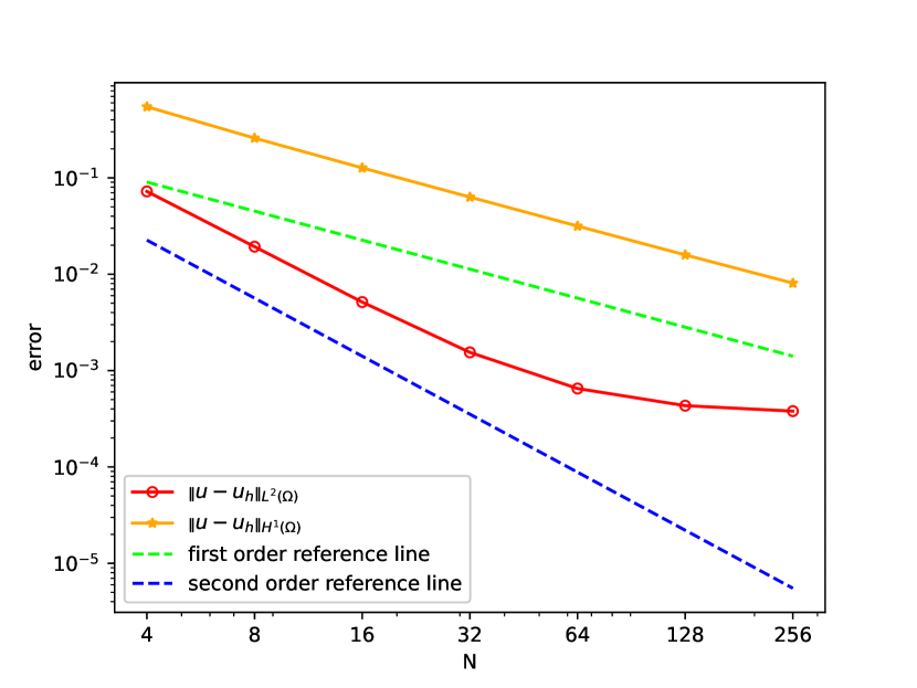
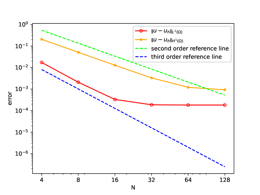
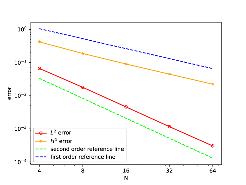
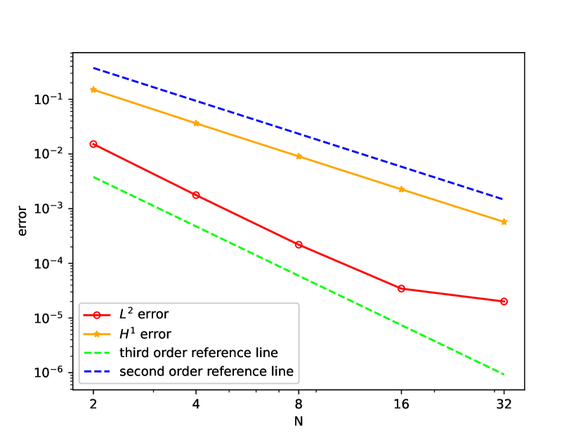
The domain is discretized using a uniform $N\times N$ grid, and tensor-product Lagrange basis functions of order $k=1$ or $2$ are employed. For convergence in $h$ , $\delta$ is fixed at $0.001$ while $N$ is progressively doubled. For convergence in $\delta$ , $h$ is fixed at $\frac{1}{128}$ (for $k=1$ ) or $\frac{1}{64}$ (for $k=2$ ), and $\delta$ is decreased from $\delta_{0}=0.04$

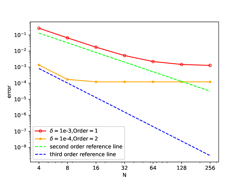
The $L^{2}$ and $H^{1}$ errors with different $h$ are shown in Figure 1 when $\delta=0.001$ . For $L^{2}$ error, the convergence rates align with the bound $O(h^{k+1})$ which is one order higher than the theoretical result. This can be attributed to the absence of Aubin-Nitsche Lemma in the nonlocal context. Similar issue is also reported in [10]. When $h\leq 1/64$ (first order element) or $h\leq 1/16$ (second order element), the $L^{2}$ error plateaus since $\delta$ dominates. For $H^{1}$ error, the observed rates are $O(h^{k})$ , though the analysis does not guarantee this due to the lack of $H^{1}$ coercivity in the nonlocal model.

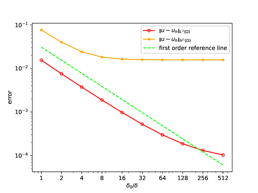
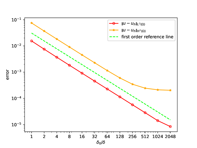
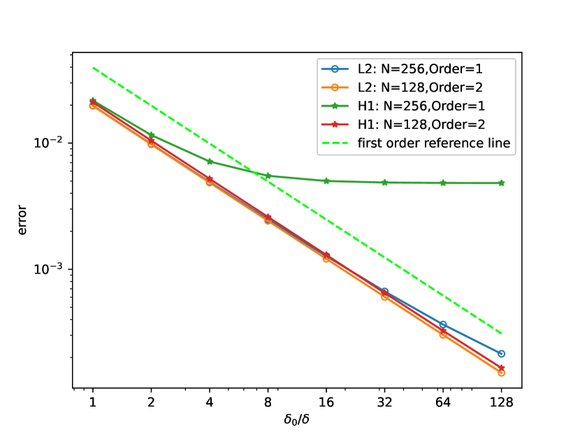
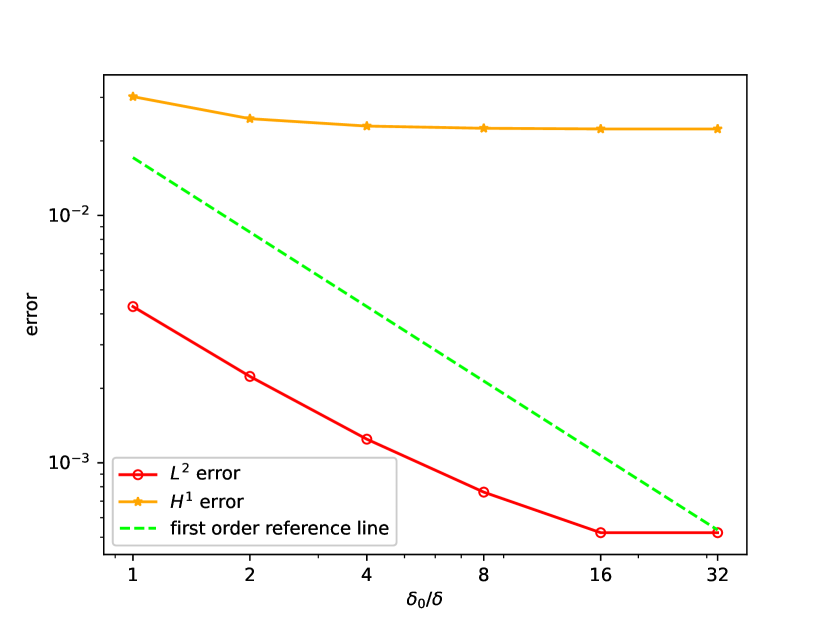
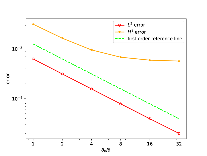
Figure 2 demonstrates the convergence in $\delta$ , confirming the first-order dependence on $\delta$ as predicted. As $\delta$ decreasing, the error also plateaus when $h$ dominates. Notably, second order elements exhibit lower plateau since high-order element achieves higher accuracy.

Refer to caption — (a) First order Lagrange interpolation

5.1.2. Errors in the gradient

In the theoretical analysis, we propose a gradient recovery technique to approximate the gradient. More precisely, we introduced $S_{\delta}u_{h}$ and $\mathbf{F}_{\delta}$ in Section 2 to approximate $\nabla u$ . In Table 1 and Table 2, we check the convergence of the gradient with respect to $h$ and $\delta$ respectively. As shown in Table 1, our method gives $k$ -th order convergence with respect to $h$ . With respect to $\delta$ , the convergence rate is first order while the rate is reduced to half order without boundary correction term $\mathbf{F}_{\delta}$ . All the numerical results fit the theoretical analysis very well.

$N$	4	8	16	32	64	128	256
1st order	5.42e-1	2.58e-1	1.27e-1	6.31e-2	3.07e-2	1.30e-2	5.54e-3
Rate	-	1.07	1.02	1.01	1.23	1.23	1.39
2nd order	5.10e-2	1.28e-2	3.46e-3	1.55e-3	1.34e-3	1.33e-3	1.33e-3
Rate	-	1.99	1.89	1.15	0.20	0.01	0.00

Table 1.

\left\|\nabla u-(\nabla S_{\delta}u_{h}-\mathbf{F}_{\delta})\right\|_{L^{2}(\Omega)}

with first and second order Lagrange Elements:

\delta=0.001

h=1/N

$\delta_{0}/\delta$	1	2	4	8	16	32
$\left\\|\nabla u-\nabla S_{\delta}u_{h}\right\\|_{L^{2}(\Omega)}$	9.97e-2	6.28e-2	4.19e-2	2.88e-2	1.99e-2	1.49e-2
Rate	-	0.67	0.58	0.54	0.53	0.42
$\left\\|\nabla u-\nabla S_{\delta}u_{h}\right\\|_{L^{2}(\Omega\backslash\Omega_{2\delta})}$	4.13e-2	2.30e-2	1.23e-2	6.24e-3	3.19e-3	1.59e-3
Rate	-	0.84	0.90	0.98	0.97	1.01
$\left\\|\nabla u-(\nabla S_{\delta}u_{h}-\mathbf{F}_{\delta})\right\\|_{L^{2}(\Omega)}$	5.93e-2	2.81e-2	1.37e-2	6.74e-3	3.35e-3	1.67e-3
Rate	-	1.08	1.04	1.02	1.01	1.01

Table 2. Gradient approximation with second order Lagrange Elements:

\delta_{0}=0.04

N=128

5.1.3. CPU time of constructing stiff matrix

Beyond convergence rate validation, we quantitatively analyzed the time consumption of stiffness matrix construction.

In Table 3, we give the CPU time of assembling the stiffness matrix with different $h$ . For uniform rectangular mesh, the stiffness matrix is translation invariant. Using this property, the computational cost can be further reduced as shown in Table 3. If the mesh is non-uniform, the translation-invariant property does not hold. In Table 3, we also list the CPU without using the translation-invariant property. As we can see, the translation-invariant property significantly reduce the computational cost.

$N=1/h$	$4$	$8$	16	32	64	128
1st order	0.004 (0.019)	0.009 (0.096)	0.025 (0.413)	0.078 (1.71)	0.695 (19.2)	5.306 (255)
2nd order	0.018 (0.170)	0.052 (0.889)	0.136 (3.898)	0.393 (16.04)	3.14 (184)	21.85 (2464)

Table 3. CPU time (in seconds) of stiffness matrix assembling with

\delta=0.01

. CPU time without using translation invariance is in the brackets.

$\delta$	$1/100$	$1/200$	$1/400$	$1/800$
1st order	5.31 (255)	2.54 (78.9)	0.939 (28.2)	0.925 (28.1)
2nd order	21.8 (2464)	10.4 (748)	4.15 (266)	4.15 (266)

Table 4. CPU time (in seconds) of stiff matrix assembling with

h=1/128

. CPU time without using translation invariance is in the brackets.

The CPU time with different $\delta$ is shown in Table 4. The computational time increases as $\delta$ grows, since more rectangles involve in the computing of local stiffness matrix.

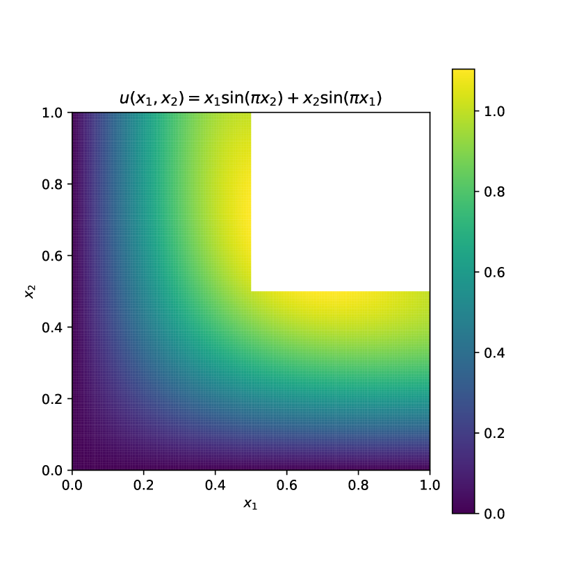
5.2. Experiments in a 2D L-shaped Region

To demonstrate the flexibility of our method for non-rectangular domains, we conduct experiments on an L-shaped region composed of two rectangular subdomains:

\Omega=[0,1]\times[0,0.5]\cup[0,0.5]\times[0.5,1].

We consider the exact solution:

u(x_{1},x_{2})=x_{1}\sin(\pi x_{2})+x_{2}\sin(\pi x_{1}),

which yields the source term:

f(x_{1},x_{2})=\pi^{2}(x_{1}\sin(\pi x_{2})+x_{2}\sin(\pi x_{1}))+u(x_{1},x_{2})

and corresponding Neumann boundary conditions. Figure 3 illustrates both the domain geometry and solution profile. The domain is discretized using a uniform Cartesian grid with special attention to the reentrant corner. The mesh ensures node alignment at $(0.5,0.5)$ by requiring even divisions in both directions.

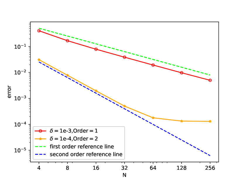
We study both the $L^{2}$ and $H^{1}$ errors between $u_{h}$ and $u$ . The results are shown in Figure 4. For L-shape region, the error has similar behavior as that in 2D box. More precisely, the numerical results verify that $\left\|u-u_{h}\right\|_{L^{2}(\Omega)}=O(h^{k+1}+\delta)$ and $\left\|u-u_{h}\right\|_{H^{1}(\Omega)}=O(h^{k}+\delta)$ .

5.3. Experiments in a 3D Cube

To demonstrate the applicability of our method in higher dimensions, we conduct numerical experiment on a 3D unit cube domain $\Omega=[0,1]\times[0,1]\times[0,1]$ . The exact solution is chosen as:

u(x_{1},x_{2},x_{3})=\cos(\pi x_{1})\cos(\pi x_{2})\cos(\pi x_{3}),

which yields the source term:

f(x_{1},x_{2},x_{3})=(1+3\pi^{2})\cos(\pi x_{1})\cos(\pi x_{2})\cos(\pi x_{3})

and homogeneous Neumann boundary conditions $g(x_{1},x_{2},x_{3})=0$ . The cubic domain is discretized using uniform partitions with $N$ subdivisions along each coordinate direction. Our implementation extends naturally from the 2D case.

Figure 5 shows the convergence behavior with fixed $\delta=10^{-4}$ and increasing mesh resolution. The observed convergence rate is $O(h^{k+1})$ in $L^{2}$ norm and $O(h^{k})$ in $H^{1}$ norm. $\delta$ -convergence is studied in Figure 6). The results confirm first-order convergence with respect to $\delta$ , with the higher-order method showing more pronounced convergence before reaching the discretization error floor.

$N=1/h$	$4$	$8$	$16$	$32$	$64$
1st order ( $\delta=0.01$ )	0.017	0.174	1.58	12.9	476
$\delta$	1/50	1/100	1/200	1/400	1/800
1st order ( $h=\frac{1}{64}$ )	1246	476	116	116	116

Table 5. CPU time (in seconds) of constructing stiff matrix with first order element in 3D.

$N=1/h$	$2$	$4$	$8$	$16$	$32$
2nd order ( $\delta=0.01$ )	0.010	0.156	1.708	15.2	128
$\delta$	0.02	0.01	0.005	0.0025	0.00125
2nd order ( $h=\frac{1}{32}$ )	550	128	128	129	128

Table 6. CPU time (in seconds) of constructing stiff matrix with second order element in 3D.

We also report the CPU time for constructing stiffness matrix in 3D case, see Table 5 and Table 6. Even for the most expensive case ( $N=64,\delta=0.02$ ), the computation can be done within 1246s in a Macbook laptop which demonstrate the efficiency of the proposed method.

6. Conclusion

This paper has presented a comprehensive framework for finite element approximation of nonlocal diffusion problems, with theoretical analysis and efficient numerical implementation. We proved that the finite element method converges to the correct local limit as both the mesh size $h$ and nonlocal horizon $\delta$ approach zero, without restrictive conditions on their relative scaling. The error analysis establishes $O(h^{k}+\delta)$ convergence in $L^{2}$ norm for shape-regular meshes using $k$ -th order elements. For problems requiring gradient approximation, we proposed a post-processing technique combining nonlocal smoothing $S_{\delta}$ with a boundary correction term $\mathbf{F}_{\delta}$ . This approach is proved to achieve $O(h^{k}+\delta)$ accuracy for the gradient approximation, overcoming the half-order loss near boundaries. Moreover, for tensor-product domains with Gaussian kernels, we introduced a novel computational strategy that decomposes the $2n$ -dimensional integrals into products of 2D integrals. This approach avoids expensive numerical quadrature while maintaining accuracy. The numerical experiments validate our theoretical results and the efficiency of the proposed algorithm across various geometries, including rectangular domains, L-shaped regions, and three-dimensional cubes.

In the future, we will try to extend this numerical method to general domain and kernels, not restrictive to the Gaussian kernel and tensor-product domain. We will also explore the application in complex problems include multiscale materials, fracture mechanics etc.

Appendices

In the following appendices, we will give the proof of Lemma 3.8 and Lemma 3.9. In the configuration of our nonlocal finite element method, the domain $\Omega$ is set to be a polyhedron. Here, for brevity of the proof, we omit some geometric details and restrict our discussion to the case where $\Omega$ is a two-dimensional rectangle. Moreover, the implementation detail for approximating $\nabla u$ is also provided.

Appendix A Proof of Lemma 3.8

To prove Lemma 3.8, a technical lemma should be introduced firstly.

Lemma A.1.

For a polyhedral $\Omega$ , let $\Omega_{\delta}=\left\{{\mathbf{x}}\big{|}d({\mathbf{x}},\partial\Omega)\leq\delta\right\}$ , then for $u\in H^{1}(\Omega)$ , we have

\displaystyle\left\|u\right\|_{L^{2}(\Omega_{\delta})}^{2}\leq C\delta\left\|u\right\|_{H^{1}(\Omega)}^{2}.

The proof of this lemma does not require any special techniques. Let $\Omega=[a_{1},b_{1}]\times[a_{2},b_{2}]$ . Following the notations in Figure 7, $\Omega_{\delta}\subset\bigcup_{i=1}^{4}\Omega_{\delta}^{i}$ .

Figure 7.

\Omega_{\delta}\subset\bigcup_{i=1}^{4}\Omega_{\delta}^{i}

Take the integral in $\Omega_{\delta}^{1}$ for example, we have

	$\displaystyle\int_{\Omega_{\delta}^{1}}u^{2}({\mathbf{x}})\mathrm{d}{\mathbf{x}}$	$\displaystyle=\int_{a_{1}}^{b_{1}}\int_{0}^{\delta}u^{2}(x_{1},x_{2})\mathrm{d}x_{2}\mathrm{d}x_{1}$
		$\displaystyle=\int_{a_{1}}^{b_{1}}\int_{0}^{\delta}\left(u(x_{1},0)+\int_{0}^{x_{2}}\partial_{2}u(x_{1},t)\mathrm{d}t\right)^{2}\mathrm{d}x_{2}\mathrm{d}x_{1}$
		$\displaystyle\leq C\int_{a_{1}}^{b_{1}}\int_{0}^{\delta}\int_{0}^{\delta}\|\partial_{2}u(x_{1},t)\|^{2}\mathrm{d}t\mathrm{d}x_{2}\mathrm{d}x_{1}+C\int_{a_{1}}^{b_{1}}\int_{0}^{\delta}u^{2}(x_{1},0)\mathrm{d}x_{2}\mathrm{d}x_{2}$
		$\displaystyle\leq C\delta\left\\|\partial_{2}u\right\\|_{L^{2}(\Omega_{\delta})}^{2}+C\delta\left\\|u\right\\|_{L^{2}(\partial\Omega)}^{2}$
		$\displaystyle\leq C\delta\left\\|u\right\\|_{H^{1}(\Omega)}^{2}.$

With this lemma, we can prove Lemma 3.8. Since

\displaystyle u({\mathbf{x}})-u({\mathbf{y}})=\int_{0}^{1}\frac{\mathrm{d}}{\mathrm{d}s}u({\mathbf{y}}+s({\mathbf{x}}-{\mathbf{y}}))\mathrm{d}s=\int_{0}^{1}\nabla u({\mathbf{y}}+s({\mathbf{x}}-{\mathbf{y}}))\cdot({\mathbf{x}}-{\mathbf{y}})\mathrm{d}s,

we have

\displaystyle\int_{\partial\Omega}\int_{\Omega}{R_{\delta}({\mathbf{x}},{\mathbf{y}})}(u({\mathbf{x}})-u({\mathbf{y}}))^{2}\mathrm{d}{\mathbf{x}}\mathrm{d}S_{\mathbf{y}}\leq C\delta^{2}\int_{0}^{1}\int_{\partial\Omega}\int_{\Omega}R_{\delta}({\mathbf{x}},{\mathbf{y}})|\nabla u({\mathbf{y}}+s({\mathbf{x}}-{\mathbf{y}}))|^{2}\mathrm{d}{\mathbf{x}}\mathrm{d}S_{\mathbf{y}}\mathrm{d}s.

For $s\in(0,1]$ ,

		$\displaystyle\int_{\partial\Omega}\int_{\Omega}R_{\delta}({\mathbf{x}},{\mathbf{y}})\|\nabla u({\mathbf{y}}+s({\mathbf{x}}-{\mathbf{y}}))\|^{2}\mathrm{d}{\mathbf{x}}\mathrm{d}S_{\mathbf{y}}$
	$\displaystyle\leq$	$\displaystyle\int_{\partial\Omega}\int_{\Omega}C_{\delta}R\left(\frac{\|{\mathbf{z}}-{\mathbf{y}}\|^{2}}{4s^{2}\delta^{2}}\right)\|\nabla u({\mathbf{z}})\|^{2}\frac{1}{s^{n}}\mathrm{d}{\mathbf{z}}\mathrm{d}S_{\mathbf{y}}$
	$\displaystyle=$	$\displaystyle C\int_{\partial\Omega}\int_{\Omega_{2s\delta}}R_{s\delta}({\mathbf{z}},{\mathbf{y}})\|\nabla u({\mathbf{z}})\|^{2}\frac{1}{s^{n}}\mathrm{d}{\mathbf{z}}\mathrm{d}S_{\mathbf{y}}$
	$\displaystyle\leq$	$\displaystyle\frac{C}{s\delta}\int_{\Omega_{2s\delta}}\|\nabla u({\mathbf{z}})\|^{2}\mathrm{d}{\mathbf{z}}$
	$\displaystyle\leq$	$\displaystyle C\left\\|u\right\\|_{H^{2}(\Omega)}^{2}.$

Here we have proved Lemma 3.8.

Appendix B Proof of Lemma 3.9

In this section, we give the proof of Lemma 3.9. From (3.22), we can get

		$\displaystyle\nabla u({\mathbf{x}})-\nabla S_{\delta}u({\mathbf{x}})+F_{\delta}({\mathbf{x}})$
	$\displaystyle=$	$\displaystyle\frac{1}{w_{\delta}({\mathbf{x}})}\int_{\Omega}R_{\delta}({\mathbf{x}},{\mathbf{y}})(\nabla u({\mathbf{x}})-\nabla u({\mathbf{y}}))\mathrm{d}{\mathbf{y}}-\frac{1}{w_{\delta}^{2}({\mathbf{x}})}\int_{\partial\Omega}\int_{\Omega}{R_{\delta}({\mathbf{x}},{\mathbf{y}})}R_{\delta}({\mathbf{x}},{\mathbf{z}})Tu({\mathbf{y}},{\mathbf{z}})n({\mathbf{z}})\mathrm{d}{\mathbf{y}}\mathrm{d}S_{\mathbf{z}}$

where

\displaystyle Tu({\mathbf{y}},{\mathbf{z}})=u({\mathbf{y}})-u({\mathbf{z}})-(({\mathbf{y}}-{\mathbf{z}})\cdot{\mathbf{n}}({\mathbf{z}}))(\nabla u({\mathbf{z}})\cdot{\mathbf{n}}({\mathbf{z}})).

The first term above has been estimated in (3.23). We will focus on the second term in this section. When $u\in C^{3}(\bar{\Omega})$ , we can divide $Tu({\mathbf{y}},{\mathbf{z}})=T_{1}u({\mathbf{y}},{\mathbf{z}})+T_{2}u({\mathbf{y}},{\mathbf{z}})$ , where

\displaystyle T_{1}u({\mathbf{y}},{\mathbf{z}})=\nabla u({\mathbf{z}})\cdot(({\mathbf{y}}-{\mathbf{z}})-(({\mathbf{y}}-{\mathbf{z}})\cdot{\mathbf{n}}({\mathbf{z}})){\mathbf{n}}({\mathbf{z}})),

and

\displaystyle T_{2}u({\mathbf{y}},{\mathbf{z}})=\int_{0}^{1}\int_{0}^{1}\sum_{i,j}\partial_{ij}u({\mathbf{z}}+st({\mathbf{y}}-{\mathbf{z}}))s(y_{i}-z_{i})(y_{j}-x_{j})\mathrm{d}t\mathrm{d}s.

With the same trick in Appendix A, we can prove

\displaystyle\left\|\frac{1}{w_{\delta}^{2}({\mathbf{x}})}\int_{\partial\Omega}\int_{\Omega}{R_{\delta}({\mathbf{x}},{\mathbf{y}})}R_{\delta}({\mathbf{x}},{\mathbf{z}})T_{2}u({\mathbf{y}},{\mathbf{z}})n({\mathbf{z}})\mathrm{d}{\mathbf{y}}\mathrm{d}S_{\mathbf{z}}\right\|_{L^{2}(\Omega)}^{2}\leq C\delta^{3}\left\|u\right\|_{H^{3}(\Omega)}^{2}.

(B.1)

To estimate the integral about $T_{1}u({\mathbf{y}},{\mathbf{z}})$ , we divide $\Omega$ into two parts. In detail, if for the polyhedron $\Omega$ , $\partial\Omega=\bigcup_{i=1}^{n}E_{i}$ , where $E_{i}$ is the flat face of the boundary of $\Omega$ , we can denote

D_{1}=\left\{{\mathbf{x}}\in\Omega_{2\delta},\text{there exists unique }i,B({\mathbf{x}},2\delta)\cap\partial\Omega\subset E_{i}\right\},

and $D_{2}=\Omega_{\delta}\backslash D_{1}$ .

For a fixed ${\mathbf{x}}\in D_{1}$ , ${\mathbf{n}}({\mathbf{z}})$ is in fact a constant vector.

		$\displaystyle{\int_{\partial\Omega}}{\int_{\Omega}}{R_{\delta}({\mathbf{x}},{\mathbf{y}})}R_{\delta}({\mathbf{x}},{\mathbf{z}})T_{1}u({\mathbf{y}},{\mathbf{z}})\mathrm{d}{\mathbf{y}}\mathrm{d}S_{\mathbf{z}}$
	$\displaystyle=$	$\displaystyle{\int_{\partial\Omega}}{\int_{\Omega}}{R_{\delta}({\mathbf{x}},{\mathbf{y}})}R_{\delta}({\mathbf{x}},{\mathbf{z}})({\mathbf{y}}-{\mathbf{z}})\cdot(I-{\mathbf{n}}({\mathbf{z}}){\mathbf{n}}({\mathbf{z}})^{T})\nabla u({\mathbf{z}})\mathrm{d}{\mathbf{y}}\mathrm{d}S_{\mathbf{z}}$
	$\displaystyle=$	$\displaystyle{\int_{\partial\Omega}}R_{\delta}({\mathbf{x}},{\mathbf{z}})({\mathbf{x}}-{\mathbf{z}})\cdot\nabla_{\Gamma}u({\mathbf{z}})\mathrm{d}S_{\mathbf{z}}{\int_{\Omega}}{R_{\delta}({\mathbf{x}},{\mathbf{y}})}\mathrm{d}{\mathbf{y}}+{\int_{\partial\Omega}}R_{\delta}({\mathbf{x}},{\mathbf{z}})\nabla_{\Gamma}u({\mathbf{z}})\mathrm{d}S_{\mathbf{z}}\cdot{\int_{\Omega}}{R_{\delta}({\mathbf{x}},{\mathbf{y}})}({\mathbf{y}}-{\mathbf{x}})\mathrm{d}{\mathbf{y}}$

For the second term, symmetry implies ${\int_{\Omega}}{R_{\delta}({\mathbf{x}},{\mathbf{y}})}({\mathbf{y}}-{\mathbf{x}})\mathrm{d}{\mathbf{y}}$ is parallel to ${\mathbf{n}}({\mathbf{z}})$ . Meanwhile, $\nabla_{\Gamma}u({\mathbf{z}})$ is orthogonal to ${\mathbf{n}}({\mathbf{z}})$ . Hence, the second term is in fact zero. As for the first term, using integration by parts on $\partial\Omega$ , we have

\displaystyle{\int_{\partial\Omega}}R_{\delta}({\mathbf{x}},{\mathbf{z}})({\mathbf{x}}-{\mathbf{z}})\cdot\nabla_{\Gamma}u({\mathbf{z}})\mathrm{d}S_{\mathbf{z}}=\delta^{2}\int_{\partial\Omega}\bar{R}_{\delta}({\mathbf{x}},{\mathbf{z}})\Delta_{\Gamma}u({\mathbf{z}})\mathrm{d}{\mathbf{z}}.

Now, we have

	$\displaystyle\int_{D_{1}}\left({\int_{\partial\Omega}}{\int_{\Omega}}{R_{\delta}({\mathbf{x}},{\mathbf{y}})}R_{\delta}({\mathbf{x}},{\mathbf{z}})T_{1}u({\mathbf{y}},{\mathbf{z}})\mathrm{d}{\mathbf{y}}\mathrm{d}S_{\mathbf{z}}\right)^{2}\mathrm{d}{\mathbf{x}}$
$\displaystyle=$	$\displaystyle\int_{D_{1}}w_{\delta}^{2}({\mathbf{x}})\left({\int_{\partial\Omega}}R_{\delta}({\mathbf{x}},{\mathbf{z}})({\mathbf{x}}-{\mathbf{z}})\cdot\nabla_{\Gamma}u({\mathbf{z}})\mathrm{d}S_{\mathbf{z}}\right)^{2}\mathrm{d}{\mathbf{x}}$
$\displaystyle\leq$	$\displaystyle C\delta^{4}\int_{D_{1}}\left(\int_{\partial\Omega}\bar{R}_{\delta}({\mathbf{x}},{\mathbf{z}})\Delta_{\Gamma}u({\mathbf{z}})\mathrm{d}S_{\mathbf{z}}\right)\mathrm{d}{\mathbf{x}}$
$\displaystyle\leq$	$\displaystyle C\delta^{3}\int_{D_{1}}\int_{\partial\Omega}\bar{R}_{\delta}({\mathbf{x}},{\mathbf{z}})(\Delta_{\Gamma}u({\mathbf{z}}))^{2}\mathrm{d}S_{\mathbf{z}}\mathrm{d}{\mathbf{x}}$
$\displaystyle\leq$	$\displaystyle C\delta^{3}\left\\|\Delta_{\Gamma}u\right\\|_{L^{2}(\partial\Omega)}^{2}$
$\displaystyle\leq$	$\displaystyle C\delta^{3}\left\\|u\right\\|_{H^{3}(\Omega)}^{2}.$	(B.2)

Figure 8. The Region

D_{2}

and

D_{2}^{1}

For ${\mathbf{x}}\in D_{2}$ , we just need to discuss each subdomain near the corners of $\Omega$ . As shown in Figure 8, we firstly take the region $D_{2}^{1}$ in the lower-left corner as an example to give the following estimation

\displaystyle\int_{D_{2}^{1}}u^{2}({\mathbf{x}})\mathrm{d}{\mathbf{x}}\leq C\delta^{2}\left\|u\right\|_{H^{2}(\Omega)}^{2},\text{ for }u\in H^{2}(\Omega).

(B.3)

The proof of this inequality is based on the Sobolev embedding. For $u\in H^{2}(\Omega)$ and the dimension of $\Omega$ to be $2$ or $3$ , we have

\displaystyle\left\|u\right\|_{C(\bar{\Omega})}\leq C\left\|u\right\|_{H^{2}(\Omega)}.

With this inequality, we can get

	$\displaystyle\int_{D_{2}^{1}}u^{2}({\mathbf{x}})\mathrm{d}{\mathbf{x}}$	$\displaystyle\leq C\int_{0}^{2\delta}\int_{0}^{2\delta}\left[\left(\int_{0}^{x_{2}}\partial_{2}u(x_{1},t)\mathrm{d}t\right)^{2}+\left(\int_{0}^{x_{1}}\partial_{1}u(s,0)\mathrm{d}s\right)^{2}\right]\mathrm{d}x_{1}\mathrm{d}x_{2}$
		$\displaystyle\hskip 56.9055pt+C\int_{0}^{2\delta}\int_{0}^{2\delta}u^{2}(0,0)\mathrm{d}x_{1}\mathrm{d}x_{2}$
		$\displaystyle\leq C\delta\int_{0}^{2\delta}\int_{0}^{2\delta}\int_{0}^{2\delta}\left(\|\partial_{2}u(x_{1},t)\|^{2}+\|\partial_{1}u(t,0)\|^{2}\right)\mathrm{d}t\mathrm{d}x_{1}\mathrm{d}x_{2}+C\delta^{2}u^{2}(0,0)$
		$\displaystyle\leq C\delta^{2}\left\\|u\right\\|_{H^{2}(\Omega)}^{2}.$

Now we can obtain

		$\displaystyle\int_{D_{2}^{1}}\left({\int_{\partial\Omega}}{\int_{\Omega}}{R_{\delta}({\mathbf{x}},{\mathbf{y}})}R_{\delta}({\mathbf{x}},{\mathbf{z}})T_{1}u({\mathbf{y}},{\mathbf{z}})\mathrm{d}{\mathbf{y}}\mathrm{d}S_{\mathbf{z}}\right)^{2}\mathrm{d}{\mathbf{x}}$
	$\displaystyle\leq$	$\displaystyle C\delta^{2}\int_{D_{2}^{1}}\left({\int_{\partial\Omega}}R_{\delta}({\mathbf{x}},{\mathbf{z}})\nabla u({\mathbf{z}})\mathrm{d}S_{\mathbf{z}}\right)^{2}\mathrm{d}{\mathbf{x}}$
	$\displaystyle\leq$	$\displaystyle C\delta\int_{D_{2}^{1}}{\int_{\partial\Omega}}R_{\delta}({\mathbf{x}},{\mathbf{z}})\|\nabla u({\mathbf{z}})-\nabla u({\mathbf{x}})\|^{2}\mathrm{d}S_{\mathbf{z}}\mathrm{d}{\mathbf{x}}+C\int_{D_{2}^{1}}\|\nabla u({\mathbf{x}})\|^{2}\mathrm{d}{\mathbf{x}}$
	$\displaystyle\leq$	$\displaystyle C\delta^{3}\left\\|u\right\\|_{H^{3}(\Omega)}^{2}+C\delta^{2}\left\\|u\right\\|_{H^{3}(\Omega)}^{2}$

In the last inequality, we used Lemma 3.8 and (B.3). Here we can conclude

\displaystyle\int_{D_{2}}\left(\int_{\partial\Omega}\int_{\Omega}R_{\delta}({\mathbf{x}},{\mathbf{y}})R_{\delta}({\mathbf{x}},{\mathbf{z}})T_{1}u({\mathbf{y}},{\mathbf{z}})\mathrm{d}{\mathbf{y}}\mathrm{d}S_{\mathbf{z}}\right)^{2}\mathrm{d}{\mathbf{x}}\leq C\delta^{2}\left\|u\right\|_{H^{3}(\Omega)}^{2}

(B.4)

Combining (3.23)(B.1)(B.2) and (B.4), Lemma 3.9 is finally proved.

Appendix C The implementation for approximating $\nabla u$

C.1. Computation of $S_{\delta}u_{h}$ .

After solving $u_{h}$ from the linear system, we can take $\nabla S_{\delta}u_{h}$ as the solution. Thus, we should also provide the method to calculate $\nabla S_{\delta}u_{h}$ .

In fact, by only a little modification in the methods above can we get the value of $\nabla S_{\delta}u_{h}({\mathbf{x}})$ for ${\mathbf{x}}\in\Omega$ . Recalling the definition in (2.10), we just need to compute

\displaystyle{\int_{\Omega}}{R_{\delta}({\mathbf{x}},{\mathbf{y}})}\mathrm{d}{\mathbf{y}}=\sum_{T^{\prime}\in\mathcal{T}_{h}}\int_{T^{\prime}}{R_{\delta}({\mathbf{x}},{\mathbf{y}})}\mathrm{d}{\mathbf{y}},\quad{\int_{\Omega}}\nabla_{\mathbf{x}}{R_{\delta}({\mathbf{x}},{\mathbf{y}})}\mathrm{d}{\mathbf{y}}=\sum_{T^{\prime}\in\mathcal{T}_{h}}\int_{T^{\prime}}\nabla_{\mathbf{x}}{R_{\delta}({\mathbf{x}},{\mathbf{y}})}\mathrm{d}{\mathbf{y}},

and

	$\displaystyle{\int_{\Omega}}{R_{\delta}({\mathbf{x}},{\mathbf{y}})}u_{h}({\mathbf{y}})\mathrm{d}{\mathbf{y}}$	$\displaystyle=\sum_{T^{\prime}\in\mathcal{T}_{h}}\sum_{i\in i(T^{\prime})}(u_{h})_{i}\int_{T^{\prime}}{R_{\delta}({\mathbf{x}},{\mathbf{y}})}\psi_{i}({\mathbf{y}})\mathrm{d}{\mathbf{y}}.$
	$\displaystyle{\int_{\Omega}}\nabla_{\mathbf{x}}{R_{\delta}({\mathbf{x}},{\mathbf{y}})}u_{h}({\mathbf{y}})\mathrm{d}{\mathbf{y}}$	$\displaystyle=\sum_{T^{\prime}\in\mathcal{T}_{h}}\sum_{i\in i(T^{\prime})}(u_{h})_{i}\int_{T^{\prime}}\nabla_{\mathbf{x}}{R_{\delta}({\mathbf{x}},{\mathbf{y}})}\psi_{i}({\mathbf{y}})\mathrm{d}{\mathbf{y}}.$

Noticing

	$\displaystyle\int_{T^{\prime}}{R_{\delta}({\mathbf{x}},{\mathbf{y}})}\mathrm{d}{\mathbf{y}}$	$\displaystyle=\left[\int_{a_{1}^{\prime}}^{b_{1}^{\prime}}e^{-\frac{s^{2}}{4\delta^{2}}(x_{1}-y_{1})^{2}}\mathrm{d}y_{1}\right]\left[\int_{a_{2}^{\prime}}^{b_{2}^{\prime}}e^{-\frac{s^{2}}{4\delta^{2}}(x_{2}-y_{2})^{2}}\mathrm{d}y_{2}\right]$
		$\displaystyle=\bar{\Phi}(a_{1}^{\prime},b_{1}^{\prime},x_{1},s/(2\delta),0)\bar{\Phi}(a_{2}^{\prime},b_{2}^{\prime},x_{2},s/(2\delta),0),$

and

		$\displaystyle\int_{T^{\prime}}\frac{\partial}{\partial x_{1}}{R_{\delta}({\mathbf{x}},{\mathbf{y}})}\psi_{i}({\mathbf{y}})\mathrm{d}{\mathbf{y}}$
	$\displaystyle=$	$\displaystyle\frac{s^{2}}{2\delta^{2}}\left[\int_{a_{1}^{\prime}}^{b_{1}^{\prime}}e^{-\frac{s^{2}}{4\delta^{2}}(x_{1}-y_{1})^{2}}(y_{1}-x_{1})p_{i1}(y_{1})\mathrm{d}y_{1}\right]\left[\int_{a_{2}^{\prime}}^{b_{2}^{\prime}}e^{-\frac{s^{2}}{4\delta^{2}}(x_{2}-y_{2})^{2}}p_{i2}(y_{2})\mathrm{d}y_{2}\right]$
	$\displaystyle=$	$\displaystyle I((y-x_{1})p_{i1},a_{1}^{\prime},b_{1}^{\prime},x_{1},s/(2\delta))I(p_{i2},a_{2}^{\prime},b_{2}^{\prime},x_{2},s/(2\delta)),$

can be reduced to the familiar integrals, the computation of $\nabla S_{\delta}u_{h}$ has been solved since the remaining necessary components can also be handled with the same way.

C.2. Computation of correction term

The correction term is defined in (2.11). Here, we illustrate the computation of this term. Similar to the calculation above, we write

	$\displaystyle\mathbf{F}_{\delta}({\mathbf{x}})$	$\displaystyle=\sum_{T\in\mathcal{T}_{h}}\sum_{L^{\prime}\in\mathcal{L}_{h}}\frac{1}{w^{2}_{\delta}({\mathbf{x}})}\int_{L^{\prime}}\int_{T}{R_{\delta}({\mathbf{x}},{\mathbf{y}})}R_{\delta}({\mathbf{x}},{\mathbf{z}})g({\mathbf{z}})(({\mathbf{y}}-{\mathbf{z}})\cdot{\mathbf{n}}({\mathbf{z}})){\mathbf{n}}({\mathbf{z}})\mathrm{d}S_{\mathbf{z}}\mathrm{d}{\mathbf{y}}$
		$\displaystyle=\sum_{T\in\mathcal{T}_{h}}\sum_{L^{\prime}\in\mathcal{L}_{h}}\sum_{i\in i(L^{\prime})}\frac{g_{i}}{w^{2}_{\delta}({\mathbf{x}})}\int_{L^{\prime}}\int_{T}{R_{\delta}({\mathbf{x}},{\mathbf{y}})}R_{\delta}({\mathbf{x}},{\mathbf{z}})\widetilde{\psi}_{i}({\mathbf{z}})(({\mathbf{y}}-{\mathbf{z}})\cdot{\mathbf{n}}({\mathbf{z}})){\mathbf{n}}({\mathbf{z}})\mathrm{d}S_{\mathbf{z}}\mathrm{d}{\mathbf{y}}$

We next take $L^{\prime}=\left\{(z_{1},z_{2})\big{|}a_{1}^{\prime}\leq z_{1}\leq b_{1}^{\prime},z_{2}=l\right\}$ and ${\mathbf{n}}({\mathbf{z}})=(0,1)^{T},{\mathbf{z}}\in L^{\prime}$ for example to explain our method. In this case, we can just consider the second decomposition

		$\displaystyle\int_{L^{\prime}}\int_{T}{R_{\delta}({\mathbf{x}},{\mathbf{y}})}R_{\delta}({\mathbf{x}},{\mathbf{z}})g({\mathbf{z}})(({\mathbf{y}}-{\mathbf{z}})\cdot{\mathbf{n}}({\mathbf{z}}))n_{2}({\mathbf{z}})\mathrm{d}{\mathbf{y}}\mathrm{d}S_{\mathbf{z}}$
	$\displaystyle=$	$\displaystyle\int_{a_{1}^{\prime}}^{b_{1}^{\prime}}\int_{a_{1}}^{b_{1}}\int_{a_{2}}^{b_{2}}e^{-\frac{s^{2}}{4\delta^{2}}[(x_{1}-y_{1})^{2}+(x_{2}-y_{2})^{2}]}e^{-\frac{s^{2}}{4\delta^{2}}[(x_{1}-z_{1})^{2}+(x_{2}-l)^{2}]}(y_{2}-l)p_{i1}(z_{1})\mathrm{d}y_{1}\mathrm{d}y_{2}\mathrm{d}z_{1}$
	$\displaystyle=$	$\displaystyle e^{-\frac{s^{2}}{4\delta^{2}}(x_{2}-l)^{2}}\int_{a_{1}^{\prime}}^{b_{2}^{\prime}}e^{-\frac{s^{2}}{4\delta^{2}}(x_{1}-z_{1})^{2}}p_{1}(z_{1})\mathrm{d}z_{1}\int_{a_{1}}^{b_{1}}e^{-\frac{s^{2}}{4\delta^{2}}(x_{1}-y_{1})^{2}}\mathrm{d}y_{1}\int_{a_{2}}^{b_{2}}e^{-\frac{s^{2}}{4\delta^{2}}(x_{2}-y_{2})^{2}}(y_{2}-l)\mathrm{d}y_{2}$
	$\displaystyle=$	$\displaystyle e^{-\frac{s^{2}}{4\delta^{2}}(x_{2}-l)^{2}}I(p_{1},a_{1}^{\prime},b_{1}^{\prime},x_{1},s/(2\delta))\Phi(a_{1}-x_{1},b_{1}-x_{1},s/(2\delta),0)I(y-l,a_{2},b_{2},x_{2},s/(2\delta)).$

Here, we once again get the required terms with some elementary integrals.

References

[1] F. Andreu-Vaillo. Nonlocal diffusion problems. Number 165. American Mathematical Soc., 2010.
[2] E. Askari, F. Bobaru, R. Lehoucq, M. Parks, S. Silling, and O. Weckner. Peridynamics for multiscale materials modeling. In Journal of Physics: Conference Series, volume 125, page 012078. IOP Publishing, 2008.
[3] S. D. Bond, R. B. Lehoucq, and S. T. Rowe. A galerkin radial basis function method for nonlocal diffusion. In Meshfree methods for partial differential equations VII, pages 1–21. Springer, 2015.
[4] C. Bucur, E. Valdinoci, et al. Nonlocal diffusion and applications, volume 20. Springer, 2016.
[5] N. Burch and R. Lehoucq. Classical, nonlocal, and fractional diffusion equations on bounded domains. International Journal for Multiscale Computational Engineering, 9(6), 2011.
[6] X. Chen and M. Gunzburger. Continuous and discontinuous finite element methods for a peridynamics model of mechanics. Computer Methods in Applied Mechanics and Engineering, 200(9-12):1237–1250, 2011.
[7] Q. Du, K. Huang, J. Scott, and W. Shen. A space-time nonlocal traffic flow model: Relaxation representation and local limit. Discrete and Continuous Dynamical Systems, 43(9):3456–3484, 2023.
[8] Q. Du, L. Ju, L. Tian, and K. Zhou. A posteriori error analysis of finite element method for linear nonlocal diffusion and peridynamic models. Mathematics of computation, 82(284):1889–1922, 2013.
[9] Q. Du, L. Tian, and X. Zhao. A convergent adaptive finite element algorithm for nonlocal diffusion and peridynamic models. SIAM Journal on Numerical Analysis, 51(2):1211–1234, 2013.
[10] Q. Du, H. Xie, X. Yin, and J. Zhang. Error estimates of finite element methods for nonlocal problems using exact or approximated interaction neighborhoods. arXiv preprint arXiv:2409.09270, 2024.
[11] Q. Du and J. Yang. Asymptotically compatible fourier spectral approximations of nonlocal allen–cahn equations. SIAM Journal on Numerical Analysis, 54(3):1899–1919, 2016.
[12] Q. Du and J. Yang. Fast and accurate implementation of fourier spectral approximations of nonlocal diffusion operators and its applications. Journal of Computational Physics, 332:118–134, 2017.
[13] Q. Du and J. Yang. Fast and accurate implementation of fourier spectral approximations of nonlocal diffusion operators and its applications. Journal of Computational Physics, 332:118–134, 2017.
[14] Q. Du and K. Zhou. Mathematical analysis for the peridynamic nonlocal continuum theory. ESAIM: Mathematical Modelling and Numerical Analysis, 45(2):217–234, 2011.
[15] M. D’Elia, M. Gunzburger, and C. Vollmann. A cookbook for approximating euclidean balls and for quadrature rules in finite element methods for nonlocal problems. Mathematical Models and Methods in Applied Sciences, 31(08):1505–1567, 2021.
[16] R. Lehoucq, F. Narcowich, S. Rowe, and J. Ward. A meshless galerkin method for non-local diffusion using localized kernel bases. Mathematics of Computation, 87(313):2233–2258, 2018.
[17] R. B. Lehoucq and S. T. Rowe. A radial basis function galerkin method for inhomogeneous nonlocal diffusion. Computer Methods in Applied Mechanics and Engineering, 299:366–380, 2016.
[18] Y. Meng and Z. Shi. Maximum principle preserving nonlocal diffusion model with dirichlet boundary condition. arXiv e-prints, pages arXiv–2310, 2023.
[19] S. Osher, Z. Shi, and W. Zhu. Low dimensional manifold model for image processing. SIAM Journal on Imaging Sciences, 10(4):1669–1690, 2017.
[20] E. Oterkus and E. Madenci. Peridynamic analysis of fiber-reinforced composite materials. Journal of Mechanics of Materials and Structures, 7(1):45–84, 2012.
[21] M. Pasetto, Z. Shen, M. D’Elia, X. Tian, N. Trask, and D. Kamensky. Efficient optimization-based quadrature for variational discretization of nonlocal problems. Computer Methods in Applied Mechanics and Engineering, 396:115104, 2022.
[22] Z. Shi, S. Osher, and W. Zhu. Weighted nonlocal laplacian on interpolation from sparse data. Journal of Scientific Computing, 73(2):1164–1177, 2017.
[23] Z. Shi and J. Sun. Convergence of the point integral method for laplace-beltrami equation on point cloud. Research in the Mathematical Sciences, 4(1):1–39, 2017.
[24] S. A. Silling and E. Askari. A meshfree method based on the peridynamic model of solid mechanics. Computers & structures, 83(17-18):1526–1535, 2005.
[25] S. A. Silling and R. B. Lehoucq. Peridynamic theory of solid mechanics. Advances in applied mechanics, 44:73–168, 2010.
[26] S. A. Silling, O. Weckner, E. Askari, and F. Bobaru. Crack nucleation in a peridynamic solid. International Journal of Fracture, 162(1):219–227, 2010.
[27] Y. Tao, Q. Sun, Q. Du, and W. Liu. Nonlocal neural networks, nonlocal diffusion and nonlocal modeling. Advances in Neural Information Processing Systems, 31, 2018.
[28] X. Tian and Q. Du. Analysis and comparison of different approximations to nonlocal diffusion and linear peridynamic equations. SIAM Journal on Numerical Analysis, 51(6):3458–3482, 2013.
[29] X. Tian and Q. Du. Asymptotically compatible schemes and applications to robust discretization of nonlocal models. SIAM Journal on Numerical Analysis, 52(4):1641–1665, 2014.
[30] J. L. Vázquez. Nonlinear diffusion with fractional laplacian operators. In Nonlinear partial differential equations, pages 271–298. Springer, 2012.
[31] T. Wang and Z. Shi. A nonlocal diffusion model with $h^{1}$ convergence for dirichlet boundary. Commun. Math. Sci., 22(7):1863–1896, 2024.
[32] X. Wang, R. Girshick, A. Gupta, and K. He. Non-local neural networks. In Proceedings of the IEEE conference on computer vision and pattern recognition, pages 7794–7803, 2018.
[33] X. Zhang, M. Gunzburger, and L. Ju. Nodal-type collocation methods for hypersingular integral equations and nonlocal diffusion problems. Computer Methods in Applied Mechanics and Engineering, 299:401–420, 2016.
[34] X. Zhang, M. Gunzburger, and L. Ju. Quadrature rules for finite element approximations of 1d nonlocal problems. Journal of Computational Physics, 310:213–236, 2016.
[35] X. Zhang, J. Wu, and L. Ju. An accurate and asymptotically compatible collocation scheme for nonlocal diffusion problems. Applied Numerical Mathematics, 133:52–68, 2018.

	$\displaystyle\left\\|L_{\delta}v\right\\|^{2}_{L^{2}(\Omega)}$	$\displaystyle\leq\frac{C}{\delta^{4}}{\int_{\Omega}}\left\|{\int_{\Omega}}{R_{\delta}({\mathbf{x}},{\mathbf{y}})}(v({\mathbf{x}})-v({\mathbf{y}}))\mathrm{d}{\mathbf{y}}\right\|^{2}\mathrm{d}{\mathbf{x}}+C{\int_{\Omega}}\left\|{\int_{\Omega}}{\bar{R}_{\delta}({\mathbf{x}},{\mathbf{y}})}v({\mathbf{y}})\mathrm{d}{\mathbf{y}}\right\|^{2}\mathrm{d}{\mathbf{x}}$
		$\displaystyle\leq\frac{C}{\delta^{4}}{\int_{\Omega}}{\int_{\Omega}}{R_{\delta}({\mathbf{x}},{\mathbf{y}})}(v({\mathbf{x}})-v({\mathbf{y}}))^{2}\mathrm{d}{\mathbf{x}}\mathrm{d}{\mathbf{y}}+C{\int_{\Omega}}{\int_{\Omega}}{\bar{R}_{\delta}({\mathbf{x}},{\mathbf{y}})}v^{2}({\mathbf{y}})\mathrm{d}{\mathbf{y}}\mathrm{d}{\mathbf{x}}$
		$\displaystyle\leq\frac{C}{\delta^{2}}\frac{1}{\delta^{2}}{\int_{\Omega}}{\int_{\Omega}}{R_{\delta}({\mathbf{x}},{\mathbf{y}})}(v({\mathbf{x}})-v({\mathbf{y}}))^{2}\mathrm{d}{\mathbf{x}}\mathrm{d}{\mathbf{y}}+C\left\\|v\right\\|_{L^{2}(\Omega)}^{2}$
		$\displaystyle\leq\frac{C}{\delta^{2}}(E_{\delta}(v))^{2}.$

	$\displaystyle\left\|{\int_{\Omega}}v({\mathbf{x}})r_{bd}({\mathbf{x}})\mathrm{d}{\mathbf{x}}\right\|$	$\displaystyle=\left\|\sum_{j=1}^{n}{\int_{\Omega}}v({\mathbf{x}}){\int_{\partial\Omega}}n^{j}({\mathbf{y}})({\mathbf{x}}-{\mathbf{y}})\cdot\nabla(\nabla^{j}u({\mathbf{y}}))\bar{R}_{\delta}({\mathbf{x}},{\mathbf{y}})\mathrm{d}S_{\mathbf{y}}\mathrm{d}{\mathbf{x}}\right\|$
		$\displaystyle\leq C\delta{\int_{\partial\Omega}}\left\\|H(u)({\mathbf{y}})\right\\|{\int_{\Omega}}{\bar{R}_{\delta}({\mathbf{x}},{\mathbf{y}})}\|v({\mathbf{x}})\|\mathrm{d}{\mathbf{x}}\mathrm{d}S_{\mathbf{y}}$
		$\displaystyle\leq C\delta\left\\|u\right\\|_{H^{2}(\partial\Omega)}\left\\|\bar{S}_{\delta}(\|v\|)\right\\|_{L^{2}(\partial\Omega)}$
		$\displaystyle\leq C\delta\left\\|u\right\\|_{H^{3}(\Omega)}\left\\|\bar{S}_{\delta}(\|v\|)\right\\|_{H^{1}(\Omega)},$

$\displaystyle\left<r_{in}+r_{bd},I_{h}u-u_{h}\right>$	$\displaystyle\leq\left\\|r_{in}\right\\|_{L^{2}(\Omega)}\left\\|I_{h}u-u_{h}\right\\|_{L^{2}(\Omega)}+C\delta\left\\|u\right\\|_{H^{3}(\Omega)}E_{\delta}(I_{h}u-u_{h})$
	$\displaystyle\leq C\delta\left\\|u\right\\|_{H^{3}(\Omega)}E_{\delta}(I_{h}u-u_{h})$
	$\displaystyle\leq C\delta\left\\|u\right\\|_{H^{3}(\Omega)}E_{\delta}(u-I_{h}u)+C\delta\left\\|u\right\\|_{H^{3}(\Omega)}E_{\delta}(e_{h})$
	$\displaystyle\leq C\delta\left\\|u\right\\|_{H^{3}(\Omega)}\left\\|u-I_{h}u\right\\|_{H^{1}(\Omega)}+C\delta\left\\|u\right\\|_{H^{3}(\Omega)}E_{\delta}(e_{h})$
	$\displaystyle\leq C\delta\frac{h^{k+1}}{\rho}\left\\|u\right\\|_{H^{3}(\Omega)}\left\\|u\right\\|_{H^{k+1}(\Omega)}+C\delta\left\\|u\right\\|_{H^{3}(\Omega)}E_{\delta}(e_{h}).$	(3.18)

$\displaystyle\left<r_{in}+r_{bd},I_{h}u-u_{h}\right>_{\Omega}$	$\displaystyle\leq\\|r_{in}\\|_{L^{2}(\Omega)}\\|I_{h}u-u_{h}\\|_{L^{2}(\Omega)}+C\delta\\|u\\|_{H^{3}(\Omega)}E_{\delta}(I_{h}u-u_{h})$
	$\displaystyle\leq C\delta\\|u\\|_{H^{3}(\Omega)}E_{\delta}(I_{h}u-u_{h})$
	$\displaystyle\leq C\delta\\|u\\|_{H^{3}(\Omega)}E_{\delta}(u-I_{h}u)+C\delta\\|u\\|_{H^{3}(\Omega)}E_{\delta}(e_{h})$
	$\displaystyle\leq C\\|u\\|_{H^{3}(\Omega)}\\|u-I_{h}u\\|_{L^{2}(\Omega)}+C\delta\\|u\\|_{H^{3}(\Omega)}E_{\delta}(e_{h})$
	$\displaystyle\leq C\delta\frac{h^{k+1}}{\delta}\\|u\\|_{H^{3}(\Omega)}\\|u\\|_{H^{k+1}(\Omega)}+C\delta\\|u\\|_{H^{3}(\Omega)}E_{\delta}(e_{h}).$	(3.19)

		$\displaystyle\int_{\partial\Omega}\int_{\Omega}R_{\delta}({\mathbf{x}},{\mathbf{y}})\|\nabla u({\mathbf{y}}+s({\mathbf{x}}-{\mathbf{y}}))\|^{2}\mathrm{d}{\mathbf{x}}\mathrm{d}S_{\mathbf{y}}$
	$\displaystyle\leq$	$\displaystyle\int_{\partial\Omega}\int_{\Omega}C_{\delta}R\left(\frac{\|{\mathbf{z}}-{\mathbf{y}}\|^{2}}{4s^{2}\delta^{2}}\right)\|\nabla u({\mathbf{z}})\|^{2}\frac{1}{s^{n}}\mathrm{d}{\mathbf{z}}\mathrm{d}S_{\mathbf{y}}$
	$\displaystyle=$	$\displaystyle C\int_{\partial\Omega}\int_{\Omega_{2s\delta}}R_{s\delta}({\mathbf{z}},{\mathbf{y}})\|\nabla u({\mathbf{z}})\|^{2}\frac{1}{s^{n}}\mathrm{d}{\mathbf{z}}\mathrm{d}S_{\mathbf{y}}$
	$\displaystyle\leq$	$\displaystyle\frac{C}{s\delta}\int_{\Omega_{2s\delta}}\|\nabla u({\mathbf{z}})\|^{2}\mathrm{d}{\mathbf{z}}$
	$\displaystyle\leq$	$\displaystyle C\left\\|u\right\\|_{H^{2}(\Omega)}^{2}.$

Asymptotically Compatible Error Bound of Finite Element Method for Nonlocal Diffusion Model with An Efficient Implementation

Abstract.

Key words and phrases:

2020 Mathematics Subject Classification:

1. Introduction

2. Nonlocal finite element discretization and main results

2.1. Nonlocal diffusion model

2.2. Finite element discretization.

2.3. Main results.

Theorem 2.1.

Remark 2.2.

Theorem 2.3.

Remark 2.4.

3. Error analysis of finite element method

3.1. Technical results.

Lemma 3.1.

Proof.

Lemma 3.2.

Proof.

Lemma 3.3.

Lemma 3.4.

3.2. Error analysis.

Lemma 3.5.

Lemma 3.6.

Proof.

3.3. Proof of Theorem 2.1.

3.4. Convergent approximation of gradient.

Lemma 3.7.

Lemma 3.8.

Lemma 3.9.

4. Fast Implementation

4.1. Computation of stiff matrix.

4.2. Computation of load vector.

5. Numerical Experiments

5.1. Experiments in a 2D rectangular region

5.1.1. Error between uu and uhu_{h}

5.1.2. Errors in the gradient

5.1.3. CPU time of constructing stiff matrix

5.2. Experiments in a 2D L-shaped Region

5.3. Experiments in a 3D Cube

6. Conclusion

Appendices

Appendix A Proof of Lemma 3.8

Lemma A.1.

Appendix B Proof of Lemma 3.9

Appendix C The implementation for approximating ∇u\nabla u

C.1. Computation of Sδ​uhS_{\delta}u_{h}.

C.2. Computation of correction term

References

5.1.1. Error between $u$ and $u_{h}$

Appendix C The implementation for approximating $\nabla u$

C.1. Computation of $S_{\delta}u_{h}$ .