Asymptotics of Network Embeddings Learned via Subsampling

\nameAndrew Davison \emailad3395@columbia.edu
\addrDepartment of Statistics
Columbia University
New York, NY 10027-5927, USA \AND\nameMorgane Austern \emailmorgane.austern@gmail.com
\addrDepartment of Statistics
Harvard University
Cambridge, MA 02138-2901, USA

Abstract

Network data are ubiquitous in modern machine learning, with tasks of interest including node classification, node clustering and link prediction. A frequent approach begins by learning an Euclidean embedding of the network, to which algorithms developed for vector-valued data are applied. For large networks, embeddings are learned using stochastic gradient methods where the sub-sampling scheme can be freely chosen. Despite the strong empirical performance of such methods, they are not well understood theoretically. Our work encapsulates representation methods using a subsampling approach, such as node2vec, into a single unifying framework. We prove, under the assumption that the graph is exchangeable, that the distribution of the learned embedding vectors asymptotically decouples. Moreover, we characterize the asymptotic distribution and provided rates of convergence, in terms of the latent parameters, which includes the choice of loss function and the embedding dimension. This provides a theoretical foundation to understand what the embedding vectors represent and how well these methods perform on downstream tasks. Notably, we observe that typically used loss functions may lead to shortcomings, such as a lack of Fisher consistency.

Keywords: networks, embeddings, representation learning, graphons, subsampling

1 Introduction

Network data are commonplace in modern-day data analysis tasks. Some examples of network data include social networks detailing interactions between users, citation and knowledge networks between academic papers, and protein-protein interaction networks, where the presence of an edge indicates that two proteins in a common cell interact with each other. With such data, there are several types of tasks we may be interested in. Within a citation network, we can classify different papers as belonging to particular subfields (a community detection task; e.g Fortunato, 2010; Fortunato and Hric, 2016). In protein-protein interaction networks, it is too costly to examine whether every protein pair will interact together (Qi et al., 2006), and so given a partially observed network we are interested in predicting the values of the unobserved edges. As users join a social network, they are recommended individuals who they could interact with (Hasan and Zaki, 2011).

A highly successful approach to solve network prediction tasks is to first learn an embedding or latent representation of the network into some manifold, usually a Euclidean space. A classical way of doing so is to perform principal component analysis or dimension reduction on the Laplacian of the adjacency matrix of the network (Belkin and Niyogi, 2003). This originates from spectral clustering methods (Pothen et al., 1990; Shi and Malik, 2000; Ng et al., 2001), where a clustering algorithm is applied to the matrix formed with the eigenvectors corresponding to the top $k$ -eigenvalues of a Laplacian matrix. One shortcoming is that for large data sets, computing the SVD of a large matrix to obtain the eigenvectors becomes increasingly computationally restrictive. Approaches which scale better for larger data sets originate from natural language processing (NLP). DeepWalk (Perozzi et al., 2014) and node2vec (Grover and Leskovec, 2016) are both network embedding methods which apply embedding methods designed for NLP, by treating various types of random walks on a graph as “sentences”, with nodes as “words” within a vocabulary. We refer to Hamilton et al. (2017b) and Cai et al. (2018) for comprehensive overviews of algorithms for creating network embeddings. See Agrawal et al. (2021) for a discussion on how such embedding methods are related to other classical methods such as multidimensional scaling, and embedding methods for other data types.

To obtain an embedding of the network, each node or vertex of the network (say $u$ ) is represented by a single $d$ -dimensional vector $\omega_{u}\in\mathbb{R}^{d}$ , which are learned by minimizing a loss function between features of the network and the collection of embedding vectors. There are several benefits to this approach. As the learned embeddings capture latent information of each node through a Euclidean vector, we can use traditional machine learning methods (such as logistic regression) to perform a downstream task. The fact that the embeddings lie within a Euclidean space also means that they are amenable to (stochastic) gradient based optimization. One important point is that, unlike in an i.i.d setting where subsamples are essentially always obtained via sampling uniformly at random, here there is substantial freedom in the way in which subsampling is performed. Veitch et al. (2018) shows that this choice has a significant influence in downstream task performance.

Despite their applied success, our current theoretical understanding of methods such as node2vec are lacking. We currently lack quantitative descriptions of what the embedding vectors represent and the information they contain, which has implications for whether the learned embeddings can be useful for downstream tasks. We also do not have quantitative descriptions for how the choice of subsampling scheme affects learned representations. The contributions of our paper in addressing this are threefold:

a)

Under the assumption that the observed network arises from an exchangeable graph, we describe the limiting distribution of the embeddings learned via procedures which depend on minimizing losses formed over random subsamples of a network, such as node2vec (Grover and Leskovec, 2016). The limiting distribution depends both on the underlying model of the graph and the choice of subsampling scheme, and we describe it explicitly for common choices of subsampling schemes, such as uniform edge sampling (Tang et al., 2015) or random-walk samplers (Perozzi et al., 2014; Grover and Leskovec, 2016).
b)

Embedding methods are frequently learned via minimizing losses which depend on the embedding vectors only through their pairwise inner products. We show that this restricts the class of networks for which an informative embedding can be learned, and that networks generated from distinct probabilistic models can have embeddings which are asymptotically indistinguishable. We also show that this can be fixed by changing the loss to use an indefinite or Krein inner product between the embedding vectors. We illustrate on real data that doing so can lead to improved performance in downstream tasks.
c)

We show that for sampling schemes based upon performing random walks on the graph, the learned embeddings are scale-invariant in the following sense. Suppose that we have two identical copies of a network generated from a sparsified exchangeable graph, and on one we delete each edge with probability $p\in(0,1)$ . Then in the limit as the number of vertices increases to infinity, the asymptotic distributions of the embedding vectors trained on the two networks will be asymptotically distinguishable. We highlight that this may provide some explanation as to the desirability of using random walk based methods for learning embeddings of sparse networks.

1.1 Motivation

We note that several approaches to learn network embeddings (Perozzi et al., 2014; Tang et al., 2015; Grover and Leskovec, 2016) do so by performing stochastic gradient updates of the embedding vectors $\omega_{i}\in\mathbb{R}^{d}$ by updates

\omega_{i}\longleftarrow\omega_{i}-\eta\frac{\partial\mathcal{L}}{\partial\omega_{i}}\quad\text{ where }\quad\mathcal{L}=-\sum_{(i,j)\in\mathcal{P}}\log\sigma\big{(}\langle\omega_{i},\omega_{j}\rangle\big{)}-\sum_{(i,j)\in\mathcal{N}}\log\big{\{}1-\sigma\big{(}\langle\omega_{i},\omega_{j}\rangle\big{)}\big{\}}.

(1)

Here $\sigma(x)=(1+e^{-x})^{-1}$ is the sigmoid function, the sets $\mathcal{P}$ and $\mathcal{N}$ are pairs of nodes which are chosen randomly at each iteration (referred to as positive and negative samples respectively) and $\eta>0$ is a step size. The goal of the objective is to force pairs of vertices within $\mathcal{P}$ to be close in the embedding space, and those within $\mathcal{N}$ to be far apart. At the most basic level, we could just have that $\mathcal{P}$ consists of edges within the graph and $\mathcal{N}$ non-edges, so that vertices which are disconnected from each other are further apart in the embedding space than those which are connected. In a scheme such as node2vec, $\mathcal{P}$ arises through a random walk on the network, and $\mathcal{N}$ arises by choosing vertices according to a unigram negative sampling distribution for each vertex in the random walk $\mathcal{P}$ .

For simplicity, assume that the only information available for training is a fully observed adjacency matrix $(a_{ij})_{i,j}$ of a network $\mathcal{G}$ of size $n$ . Moreover, we let $\mathcal{P}$ and $\mathcal{N}$ be random sets which consist only of pairs of vertices which are connected ( $a_{ij}=1$ ) and not connected ( $a_{ij}=0$ ) respectively. In this case, if we write $S(\mathcal{G})=\mathcal{P}\cup\mathcal{N}$ , then the algorithm scheme described in (1) arises from trying to minimize the empirical risk function (which depends on the underlying graph $\mathcal{G}$ )

\mathcal{R}_{n}(\omega_{1},\ldots,\omega_{n}):=\sum_{i\neq j}\mathbb{P}\big{(}(i,j)\in S(\mathcal{G})\,|\,\mathcal{G}\big{)}\ell\big{(}\langle\omega_{i},\omega_{j}\rangle,a_{ij}\big{)}

(2)

with a stochastic optimization scheme (Robbins and Monro, 1951), where we write $\ell(y,x)=-x\log\sigma(y)-(1-x)\log(1-\sigma(y))$ for the cross entropy loss.

This means that the optimization scheme in (1) attempts to find a minimizer $(\widehat{\omega}_{1},\ldots,\widehat{\omega}_{n})$ of the function $\mathcal{R}_{n}(\omega_{1},\ldots,\omega_{n})$ defined in (2). We ask several questions about these minimizers where there is currently little understanding:

Q1:

To what extent is there a unique minimizer to the empirical risk (2)?
Q2:

Does the distribution of the learnt embedding vectors $(\widehat{\omega}_{1},\ldots,\widehat{\omega}_{n})$ change as a result of changing the underlying sampling scheme? If so, can we describe quantitatively how?
Q3:

During learning of the embedding vectors, are we using a loss which limits the information we can capture in a learned representation? If so, can we fix this in some way?

Answering these questions allow us to evaluate the impact of various heuristic choices made in the design of algorithms such as node2vec, where our results will allow us to describe the impact with respect to downstream tasks such as edge prediction. We go into more depth into these questions below, and discuss in Section 1.5 how our main results help address these questions.

1.1.1 Uniqueness of minimizers of the empirical risk

We highlight that the loss and risk functions in (1) and (2) are invariant under any joint transformation of the embedding vectors $\omega_{i}\to Q\omega_{i}$ by an orthogonal matrix $Q$ . As a result, we can at most ask whether the gram matrix $\Omega_{ij}=\langle\omega_{i},\omega_{j}\rangle$ induced by the embedding vectors is uniquely characterized. This is challenging as the embedding dimension $d$ is significantly less than the number of vertices $n$ - even for networks involving millions of nodes, the embedding dimensions used by practitioners are of the order of magnitude of hundreds. As a result the gram matrix is rank constrained. Consequently, when reformulating (2) to optimize over the matrix $\Omega$ , the optimization domain is non-convex, meaning answering this question is non-trivial. Answering this allows us to understand whether the embedding dimension fundamentally influences the representation we are learning, or instead only influences how accurately we can learn such a representation.

1.1.2 Dependence of embeddings on the sampling scheme choice in learning

While we know that random-walk schemes such as node2vec are empirically successful, there has been little discussion as to how the representation learnt by such schemes compares to (for example) schemes where we sample vertices randomly and look at the induced subgraph. This is useful for understanding their performance on downstream tasks such as community detection or link prediction. Another useful example is for when embeddings are used for causal inference (Veitch et al., 2019), where there is the needed to validate assumptions that the embeddings containing information relevant to the prediction of propensity scores and expected outcomes. A final example arises in methods which try and attempt to “de-bias” embeddings through the use of adaptive sampling schemes (Rahman et al., 2019), to understand what extent they satisfy different fairness criteria.

We are also interested in understanding how the hyperparameters of a sampling scheme affect the expected value and variance of gradient estimates when performing stochastic gradient descent. The distinction is important, as the expected value influences the empirical risk being minimized - therefore the underlying representation - and the variance the speed at which an optimization algorithm converges (Dekel et al., 2012). When using stochastic gradient descent in an i.i.d data setting, the mini-batch size does not effect the expected value of the gradient estimate given the observed data, but only its variance, which decreases as the mini-batch size increases. However, for a scheme like node2vec, it is not clear whether hyperparameters such as the random walk length, or the unigram parameter affect the expectation or variance of the gradient estimates (conditional on the graph $\mathcal{G}$ ).

1.1.3 Information-limiting loss functions

One important property of representations which make them useful for downstream tasks are their ability to differentiate between different graph structures. One way to examine this is to consider different probabilistic models for a network, and to then examine whether the resulting embeddings are distinguishable from each other. If they are not, then this suggests some information about the network has been lost in learning the representation. By examining the range of distributions which have the same learned representation, we can understand this information loss and the effect on downstream task performance.

1.2 Overview of results

1.2.1 Embedding methods implicitly fit graphon models

We highlight that the loss in (2) is the same as the loss obtained by maximizing the log-likelihood formed by a probabilistic model for the network of the form

\begin{split}a_{ij}\,|\,\omega_{i},\omega_{j}&\sim\mathrm{Bernoulli}\big{(}\sigma(\langle\omega_{i},\omega_{j}\rangle)\big{)}\text{ independently for $i\neq j$}\\ \omega_{i}&\sim\mathrm{Unif}(C)\text{ independently for $i\in[n]$,}\end{split}

(3)

using stochastic gradient ascent. Here $C\subseteq\mathbb{R}^{d}$ is a closed set corresponding to a constrained set for the embedding vectors. In the limit as the number of vertices increases to infinity, such a model corresponds to an exchangeable graph (Lovász, 2012), as the infinite adjacency matrices are invariant to a permutation of the labels of the vertices.

In an exchangeable graph, each vertex $u$ has a latent feature $\lambda_{u}\sim\mathrm{Unif}[0,1]$ , with edges arising independently with $a_{uv}\,|\,\lambda_{u},\lambda_{v}\sim\mathrm{Bernoulli}(W(\lambda_{u},\lambda_{v}))$ for a function $W:[0,1]^{2}\to[0,1]$ called a graphon; see Lovász (2012) for an overview. Such models can be thought of as generalizations of a stochastic block model (Holland et al., 1983), which have a correspondence to when the function $W$ is a piecewise constant function on sets $A_{i}\times A_{j}$ for some partition $(A_{i})_{i\in[k]}$ of $[0,1]$ , with the partitions acting as the different communities within the SBM. If $\pi_{i}$ is the size of $A_{i}$ , and we write $W_{ij}$ for the value of $W(l,l^{\prime})$ on $A_{i}\times A_{j}$ , this is equivalent to the usual presentation of a stochastic block model

c(u)\stackrel{{\scriptstyle\text{i.i.d}}}{{\sim}}\mathrm{Categorical}(\pi),\qquad a_{uv}\,|\,c(u),c(v)\stackrel{{\scriptstyle\text{indep}}}{{\sim}}\mathrm{Bernoulli}(W_{c(u),c(v)}).

(4)

where $c(i)$ is the community label of vertex $u$ . One can also consider sparsified exchangeable graphs, where for a graph on $n$ vertices, edges are generated with probability $W_{n}(\lambda_{u},\lambda_{v})=\rho_{n}W(\lambda_{u},\lambda_{v})$ for a graphon $W$ and a sparsity factor $\rho_{n}\to 0$ as $n\to\infty$ . This accounts for the fact that most real world graphs are not “dense” and do not have the number of edges scaling as $O(n^{2})$ ; in a sparsified graphon, the number of edges now scales as $O(\rho_{n}n^{2})$ .

For the purposes of theoretical analysis, we look at the minimizers of (2) when the network $\mathcal{G}$ arises as a finite sample observation from a sparsified exchangeable graph whose graphon is sufficiently regular. We then examine statistically the behavior of the minimizers as the number of vertices grows towards infinity. As embedding methods are frequently used on very large networks, a large sample statistical analysis is well suited for this task. One important observation is that even when the observed data is from a sparse graph, embedding methods which fall under (3) are implicitly fitting a dense model to the data. As we know empirically that embedding methods such as node2vec produce useful representations in sparse settings, we introduce the sparsity to allow some insight as to how this can occur.

1.2.2 Types of results obtained

We now discuss our main results, with a general overview followed by explicit examples. In Theorems 10 and 19, we show that under regularity assumptions on the graphon, in the limit as the number of vertices increases to infinity, we have for any sequence of minimizers $(\widehat{\omega}_{1},\ldots,\widehat{\omega}_{n})$ to $\mathcal{R}_{n}(\omega_{1},\ldots,\omega_{n})$ that

\frac{1}{n^{2}}\sum_{i,j}\big{|}\langle\widehat{\omega}_{i},\widehat{\omega}_{j}\rangle-K(\lambda_{i},\lambda_{j})\big{|}=O_{p}(r_{n})

(5)

for a function $K:[0,1]^{2}\to\mathbb{R}$ we determine, and rate $r_{n}\to 0$ . Both $K$ and $r_{n}$ depend on the graphon $W$ and the choice of sampling scheme. The rate also depends on the embedding dimension $d$ ; we note that our results may sometimes require $d\to\infty$ as $n\to\infty$ in order for $r_{n}\to 0$ , but will always do so sub-linearly with $n$ . As a result (5) allows us to guarantee that on average, the inner products between embedding vectors contain some information about the underlying structure of the graph, as parameterized through the graphon function $W$ . One notable application of this type of result is that it allows us to give guarantees for the asymptotic risk on edge prediction tasks, when using the values $S_{ij}=\langle\widehat{\omega}_{i},\widehat{\omega}_{j}\rangle$ as scores to threshold for whether there is the presence of an edge $(i,j)$ in the graph. Our results apply to sparsified exchangeable graphs whose graphons are either piecewise constant (corresponding to a stochastic block model), or piecewise Hölder continuous.

To show how our results address the questions introduced in Section 1.1, and to highlight the connection with using the embedding vectors for edge prediction tasks, we give explicit examples (with minimal additiional notation) of results which can be obtained from the main theorems of the paper. For the remainder of the section, suppose that

\ell(y,x):=-x\log(\sigma(y))-(1-x)\log(1-\sigma(y))\qquad\qquad\Big{(}\text{with }\sigma(y)=\frac{e^{y}}{1+e^{y}}\Big{)}

denotes the cross-entropy loss function (where $y\in\mathbb{R}$ and $x\in\{0,1\}$ ). We consider graphs which arise from a sub-family of stochastic block models - frequently called SBM $(p,q,\kappa)$ models - where a graph of size $n$ is generated via the probabilistic model

c(u)\stackrel{{\scriptstyle\text{i.i.d}}}{{\sim}}\mathrm{Unif}(\{1,\ldots,\kappa\}),\qquad a_{uv}\,|\,c(u),c(v)\stackrel{{\scriptstyle\text{indep}}}{{\sim}}\begin{cases}\mathrm{Bernoulli}(\rho_{n}p)&\text{ if }c(u)=c(v),\\ \mathrm{Bernoulli}(\rho_{n}q)&\text{ if }c(u)\neq c(v).\end{cases}

(6)

Here $\rho_{n}$ is a sparsifying sequence. For our results below, we will consider the cases when $\rho_{n}=1$ or $\rho_{n}=(\log n)^{2}/n$ (so $\rho_{n}\to 0$ in the second case). With regards to the choice of sampling schemes, we consider two choices:

i)

Uniform vertex sampling: A sampling scheme where we select $100$ vertices uniformly at random, and then form a loss over the induced sub-graph formed by these vertices.
ii)

node2vec: The sampling scheme in node2vec where we use a walk length of $50$ , select $1$ negative samples per vertex using a unigram distribution with $\alpha=0.75$ . (See either Grover and Leskovec (2016), or Algorithm 4 in Section 4, for more details.)

Recall that defining a sampling scheme and a loss function induces a empirical risk as given in (2), with the sampling scheme defining sampling probabilities $\mathbb{P}((u,v)\in S(\mathcal{G})\,|\,\mathcal{G})$ . Below we will give theorem statements for two types of empirical risks, depending on how we combine two embedding vectors $\omega_{u}$ and $\omega_{v}$ to give a scalar. The first uses a regular positive definite inner product $\langle\omega_{u},\omega_{v}\rangle$ , and the second uses a Krein inner product, which takes the form $\langle\omega_{u},S\omega_{v}\rangle$ where $S$ is a diagonal matrix with entries $\{+1,-1\}$ .

Supposing we have embedding vectors $\omega_{u}\in\mathbb{R}^{2d}$ , we consider the risks

	$\displaystyle\mathcal{R}_{n}(\omega_{1},\ldots,\omega_{n})$	$\displaystyle:=\sum_{i\neq j}\mathbb{P}\big{(}(i,j)\in S(\mathcal{G})\,\|\,\mathcal{G}\big{)}\ell\big{(}\langle\omega_{i},\omega_{j}\rangle,a_{ij}\big{)},$		(7)
	$\displaystyle\mathcal{R}^{B}_{n}(\omega_{1},\ldots,\omega_{n})$	$\displaystyle:=\sum_{i\neq j}\mathbb{P}\big{(}(i,j)\in S(\mathcal{G})\,\|\,\mathcal{G}\big{)}\ell\big{(}\langle\omega_{i},S_{d}\,\omega_{j}\rangle,a_{ij}\big{)},$		(8)

where $S_{d}=\mathrm{diag}(I_{d},-I_{d})\in\mathbb{R}^{2d\times 2d}$ and $I_{d}\in\mathbb{R}^{d\times d}$ is the $d$ -dimensional identity matrix. With this, we are now in a position to state results of the form given in (5). As it is easier to state results when using the second risk $\mathcal{R}^{B}_{n}(\omega_{1},\ldots,\omega_{n})$ , we will begin with this, and state two results corresponding to either the uniform vertex sampling scheme, or the node2vec sampling scheme. We then discuss implications of the results afterwards.

Theorem 1

Suppose that we use the uniform vertex sampling scheme described above, we choose the embedding dimension $d=2\kappa$ , and $\rho_{n}=1$ for all $n$ . Then for any sequence of minimizers $(\widehat{\omega}_{1},\ldots,\widehat{\omega}_{n})$ to $\mathcal{R}^{B}_{n}(\omega_{1},\ldots,\omega_{n})$ , we have that

\frac{1}{n^{2}}\sum_{i,j}\big{|}\langle\widehat{\omega}_{i},S_{d}\,\widehat{\omega}_{j}\rangle-K_{c(i),c(j)}\big{|}\to 0

in probability as $n\to\infty$ , where $K\in\mathbb{R}^{\kappa\times\kappa}$ is the matrix

K_{lm}=\begin{cases}\log(p/(1-p))&\text{ if }l=m,\\ \log(q/(1-q))&\text{ if }l\neq m\end{cases}

Theorem 2

Suppose in Theorem 1 we instead use the node2vec sampling scheme described earlier, and now either $\rho_{n}=1$ or $\rho_{n}=(\log n)^{2}/n$ . Then the same convergence guarantee holds, except now the matrix $K\in\mathbb{R}^{\kappa\times\kappa}$ takes the form

	$\displaystyle K_{lm}$	$\displaystyle=\log\Big{(}\frac{p\kappa}{1.02(1-\rho_{n}p)(p+(\kappa-1)q}\Big{)}\qquad\text{ if }l=m,$
		$\displaystyle=\log\Big{(}\frac{q\kappa}{1.02(1-\rho_{n}q)(p+(\kappa-1)q}\Big{)}\qquad\text{ if }l\neq m.$

With these two results, we make a few observations:

i)

In our convergence theorems, we say that for any sequence of minimizers, the matrix $(\langle\widehat{\omega}_{i},S_{d}\,\widehat{\omega}_{j}\rangle)_{i,j}$ will have the same limiting distribution. Although here we explicitly choose $d=2\kappa$ , $d$ can be any sequence which which diverges to infinity (provided it does so sufficiently slowly) and have the same result hold. Consequently, this suggests that up to symmetry and statistical error, the minimizers of the empirical risk will be essentially unique, giving an answer to Q1.
ii)

For different sampling schemes, we are able to give a closed form description of the limiting distribution of the matrices $(\langle\widehat{\omega}_{i},S_{d}\,\widehat{\omega}_{j}\rangle)_{i,j}$ , and we can see that they are different for different sampling schemes. This affirms Q2 as posed above in the positive. One interesting observation from the Theorems 1 and 2 is the dependence on the sparsity factor. While a uniform vertex sampling scheme does not work well in the sparsified setting (and so we give convergence results only when $\rho_{n}=1$ ) in node2vec the representation remains stable in the limit when $\rho_{n}\to 0$ .
iii)

Theorem 1 tells us that if we use a uniform sampling scheme, then using the Krein inner product during learning and the $S_{ij}=\langle\widehat{\omega}_{i},S_{d}\widehat{\omega}_{j}\rangle$ as scores, we are able to perform edge prediction up to the information theoretic threshold.
iv)

If in Theorem 2 we instead let the walk length in node2vec to be of length $k$ , the $1.02$ term in the limiting distribution for node2vec would be replaced by $1+k^{-1}$ . This means that in the limit $k\to\infty$ , the limiting distribution is independent of the walk length. We discuss later in Section 4.1 the roles of the hyperparameters in node2vec, and argue that the walk length places a role in only reducing the variance of gradient estimates.

So far we have only given results for minimizers of the loss $\mathcal{R}^{B}_{n}(\omega_{1},\ldots,\omega_{n})$ . We now give an example of a convergence result for $\mathcal{R}_{n}(\omega_{1},\ldots,\omega_{n})$ , and afterwards discuss how this result addresses Q3 as posed above.

Theorem 3

Suppose the graph arises from a SBM( $p,q,2$ ) model. Let $\sigma^{-1}(y)=\log(y/(1-y)$ denote the inverse sigmoid function. Suppose that we use the uniform vertex sampling scheme described above, the embedding dimension satisfies $d\geq 2$ and $\rho_{n}=1$ . Then for any sequence of minimizers $(\widehat{\omega}_{1},\ldots,\widehat{\omega}_{n})$ to $\mathcal{R}_{n}(\omega_{1},\ldots,\omega_{n})$ , we have that

\frac{1}{n^{2}}\sum_{i,j}\big{|}\langle\widehat{\omega}_{i},\widehat{\omega}_{j}\rangle-K_{c(i),c(j)}\big{|}=o_{p}(1)\qquad\text{ where }K=\begin{pmatrix}K_{11}&K_{12}\\ K_{12}&K_{11}\end{pmatrix}

and the values of $K_{11}$ and $K_{12}$ depend on $p$ and $q$ as follows:

a)

If $p\geq q$ and $p+q\geq 1$ , then $K_{11}=\sigma^{-1}(p)$ and $K_{12}=\sigma^{-1}(q)$ ;
b)

If $p\geq q$ and $p+q<1$ , then $K_{11}=-K_{12}=\sigma^{-1}((1+p-q)/2)$ ;
c)

If $p<q$ and $p+q\geq 1$ , then $K_{11}=K_{12}=\sigma^{-1}((p+q)/2)$ ;
d)

Otherwise, $K_{11}=K_{12}=0$ .

From the above theorem we can see that the representation produced is not an invertible function of the model from which the data arose. For example in the regime where $p\geq q$ and $p+q<1$ , the representation depends only on the size of the gap $p-q$ , and so one can choose different values of $(p,q)$ for which the limiting distribution is the same. This answers the first part of Q3. (We discuss this further in Section 3.4; see the discussion after Proposition 20.) In contrast, this does not occur in Theorem 1 - the representation learned is an invertible function of the underlying model. Theorem 3 also highlights that, when using only the regular inner product during training and scores $S_{ij}=\langle\widehat{\omega}_{i},\widehat{\omega}_{j}\rangle$ , there are regimes (such as when $p<q$ ) where the scores produced will be unsuitable for purposes of edge prediction.

The fundamental difference between Theorems 1 and 3 is that the risk $\mathcal{R}_{n}^{B}(\omega_{1},\ldots,\omega_{n})$ we consider in Theorem 1 arises by making the implicit assumption that the network arises from a probabilistic model $a_{ij}\,|\,\omega_{i},\omega_{j}\sim\mathrm{Bernoulli}\big{(}\sigma(\langle\omega_{i},S_{d}\,\omega_{j}\rangle)\big{)}$ . This means the inverse-logit matrix of edge probabilities are not constrained to be positive-definite, whereas using $\langle\omega_{i},\omega_{j}\rangle$ as in (3) to give $\mathcal{R}_{n}(\omega_{1},\ldots,\omega_{n})$ places a positive-definite constraint on this matrix. This can be interpreted as a form of model misspecification of the data generating process. To address the information loss which occurs when parameterizing the loss through inner products $\langle\omega_{i},\omega_{j}\rangle$ , we can fix this by replacing it with a Krein inner product. This gives an answer to the second part of Q3. We later demonstrate that making this change can lead to improved performance when using the learned embeddings for downstream tasks on real data (Section 5.2), suggesting these findings are not just an artefact of just the type of models we consider.

1.3 Related works

There is a large literature looking at embeddings formed via spectral clustering methods under various network models from a statistical perspective; see e.g Ma et al. (2021); Deng et al. (2021) for some recent examples. For models supporting a natural community structure, these frequently take the form of giving guarantees on the behavior of the embeddings, and then argue that using a clustering method with the embedding vectors allows for weak/strong consistency of community detection. See Abbe (2017) for an overview of the information theoretic thresholds for the different type of recovery guarantees.

Lei and Rinaldo (2015) consider spectral clustering using the eigenvectors of the adjacency matrix for a stochastic block model. Rubin-Delanchy et al. (2017) consider spectral embeddings using both the adjacency matrix and Laplacian matrices from models arising from generative models of the form $A_{ij}|X_{i},X_{j}\sim\mathrm{Bernoulli}(\langle X_{i},I_{p,q}X_{j}\rangle)$ where $I_{p,q}=\mathrm{diag}(I_{p},-I_{q})$ ) and the $X_{i}\in\mathbb{R}^{d}$ are i.i.d random variables with $p,q,d$ known and fixed - such graphs are referred to frequently as dot product graphs. These allow for a broader class of models than stochastic block models, such as mixed-membership models. The $q=0$ case was considered by Tang and Priebe (2018), with central limit theorem results given in Levin et al. (2021); see Athreya et al. (2018) for a broader review of statistical analyses of various methods on these graphs. In Lei (2021), they consider similar models where $A_{ij}|Z_{i},Z_{j}\sim\mathrm{Bernoulli}(\langle Z_{i},Z_{j}\rangle_{\mathcal{K}})$ where $\mathcal{K}$ is a Krein space (formally, this is a direct sum of Hilbert spaces equipped with an indefinite inner product, formed by taking the difference of the inner products on the summand Hilbert spaces), with their results applying to non-negative definite graphons and graphons which are Hölder continuous for exponents $\beta>1/2$ . They then discuss the estimation of the $Z_{i}$ using the eigendecomposition of the adjacency matrix (which we have noted can be viewed as a type of embedding) from a functional data analysis perspective. We note that in our work we do not directly assume a model of such a form, but some of our proofs use some similar ideas.

With regards to embeddings learned via random walk approaches such as node2vec (Grover and Leskovec, 2016), there are a few works which study modified loss functions. To be precise, these suppose that each vertex $u$ has two embedding vectors $\omega_{u}\in\mathbb{R}^{d}$ and $\eta_{u}\in\mathbb{R}^{d}$ , with terms of the form $\langle\omega_{i},\omega_{j}\rangle$ replaced in the loss with $\langle\omega_{i},\eta_{j}\rangle$ , and $\omega_{u}$ , $\eta_{u}$ are allowed to vary independently with each other. Qiu et al. (2018) study several different embedding methods within this context (including those involving random walks) where they explicitly write down the closed form of the minimizing matrix $(\langle\omega_{i},\eta_{j}\rangle)_{ij}$ for the loss having averaged over the random walk process when $d\geq n$ and $n$ is fixed. In order to be always able to write down explicitly the minimizing matrix, they rely on the assumption that $d\geq n$ and that $\eta_{j}$ and $\omega_{j}$ are unconstrained of each other, so that the matrix $(\langle\omega_{i},\eta_{j}\rangle)_{ij}$ is unconstrained. This avoids the issues of non-convexity in the problem. We note that in our work we are able to handle the case where we enforce the constraints $\eta_{j}=\omega_{j}$ (as in the original node2vec paper) and $d\ll n$ , so we address the non-convexity.

Zhang and Tang (2021) then considers the same minimizing matrix as in Qiu et al. (2018) for stochastic block models, and examines the best rank $d$ approximation (with respect to the Frobenius norm) to this matrix, in the regime where $n\to\infty$ and $d$ is less than or equal to the number of communities. We comment that our work gives convergence guarantees under broad families of sampling schemes, including - but not limited to - those involving random walks, and for general smooth graphons rather than only stochastic block models. Veitch et al. (2018) discusses the role of subsampling as a model choice, within the context of specifying stochastic gradient schemes for empirical risk minimization for learning network representations, and highlights the role they play in empirical performance.

1.4 Notation and nomenclature

For this section, we write $\mu$ for the Lebesgue measure, $\mathrm{int}(A)$ the interior of a set $A$ and $\mathrm{cl}(A)$ as the closure of $A$ . We say that a partition $\mathcal{Q}$ of $X\subseteq\mathbb{R}^{d}$ , written $\mathcal{Q}=(Q_{1},\ldots,Q_{\kappa})$ , is a finite collection of pairwise disjoint, connected sets whose union is $X$ , and $\mu(\mathrm{int}(Q))>0$ and $\mu(\mathrm{cl}(Q)\setminus\mathrm{int}(Q))=0$ for all $Q\in\mathcal{Q}$ . For a partition $\mathcal{Q}$ of $X$ , we define

\mathcal{Q}^{\otimes 2}:=\{Q_{i}\times Q_{j}\,:\,Q_{i},Q_{j}\in\mathcal{Q}\},

which gives a partition of $X^{2}$ . A refinement $\mathcal{Q}^{\prime}$ of $\mathcal{Q}$ is a partition $\mathcal{Q}^{\prime}$ where for every $Q^{\prime}\in\mathcal{Q}^{\prime}$ , there exists a (necessarily unique) $Q\in\mathcal{Q}$ such that $Q^{\prime}\subseteq Q$ .

We say a function $f:X\to\mathbb{R}$ is Hölder $(X,\beta,M)$ , where $X\subseteq[0,1]^{d}$ is closed and $\beta\in(0,1]$ , $M>0$ are constants, if

|f(x)-f(y)|\leq M\|x-y\|_{2}^{\beta}\qquad\text{ for all }x,y\in X.

We say a function $f:X\to\mathbb{R}$ is piecewise Hölder $(X,\beta,M,\mathcal{Q})$ if the following holds: for any $Q\in\mathcal{Q}$ , the restriction $f|_{Q}$ admits a continuous extension to $\mathrm{cl}(Q)$ , with this extension being Hölder $(\mathrm{cl}(Q),\beta,M)$ . Similarly, we say that a function $f:X\to\mathbb{R}$ is piecewise continuous on $\mathcal{Q}$ if for every $Q\in\mathcal{Q}$ , $f|_{Q}$ admits a continuous extension to $\mathrm{cl}(Q)$ .

For a graph $\mathcal{G}=(\mathcal{V},\mathcal{E})$ with vertex set $\mathcal{V}\subseteq\mathbb{N}$ and edge set $\mathcal{E}$ , we let $A=(a_{uv})_{u,v\in\mathcal{V}}$ denote the adjacency matrix of $\mathcal{G}$ , so $a_{uv}=1$ iff $(u,v)\in\mathcal{E}$ . Here we consider undirected graphs with no self-loops, so $(u,v)\in\mathcal{E}\iff(v,u)\in\mathcal{E}$ ; we count $(u,v)$ and $(v,u)$ together as one edge. For such a graph, we let

•

$E[\mathcal{G}]=\sum_{u<v}a_{uv}=\frac{1}{2}\sum_{u\neq v}a_{uv}$ denote the number of edges of $\mathcal{G}$ ;
•

$\mathrm{deg}(u)=\sum_{v}a_{uv}$ denotes the degree of the vertex $u$ , so $\sum_{u}\mathrm{deg}(u)=2E[\mathcal{G}]$ .

A subsample $S(\mathcal{G})$ of a graph $\mathcal{G}$ is a collection of vertices $\mathcal{V}(S(\mathcal{G}))$ , along with a symmetric subset of the adjacency matrix of $\mathcal{G}$ restricted to $\mathcal{V}(S(\mathcal{G}))$ ; that is, a subset of $(a_{uv})_{u,v\in\mathcal{V}(S(\mathcal{G}))}$ . The notation $(i,j)\in S(\mathcal{G})$ therefore refers to whether $a_{ij}$ is an element of the aforementioned subset of $(a_{uv})_{u,v\in\mathcal{V}(S(\mathcal{G}))}$ .

In the paper, we consider sequences of random graphs $(\mathcal{G}_{n})_{n\geq 1}$ generated by a sequence of graphons $(W_{n})_{n\geq 1}$ . A graphon is a symmetric measurable function $W:[0,1]^{2}\to[0,1]$ . To generate these graphs, we draw latent variables $\lambda_{i}\sim U[0,1]$ independently for $i\in\mathbb{N}$ , and then for $i<j$ set

a^{(n)}_{ij}|\lambda_{i},\lambda_{j}\sim\mathrm{Bernoulli}(W_{n}(\lambda_{i},\lambda_{j}))

independently, and $a^{(n)}_{ji}=a^{(n)}_{ij}$ for $j<i$ . We then let $\mathcal{G}_{n}$ be the graph formed with adjacency matrix $A^{(n)}$ restricted to the first $n$ vertices. Unless mentioned otherwise, we understand that references to $\lambda_{i}$ and $a_{ij}$ - now dropping the superscript $(n)$ - refer to the above generative process. For a graphon $W$ , we will denote

•

$\mathcal{E}_{W}=\int_{0}^{1}\int_{0}^{1}W(l,l^{\prime})\;dl\,dl^{\prime}$ for the edge density of $W$ ;
•

$W(\lambda,\cdot)=\int_{0}^{1}W(\lambda,y)\,dy$ for the degree function of $W$ ;
•

$\mathcal{E}_{W}(\alpha)=\int_{0}^{1}W(\lambda,\cdot)^{\alpha}\,d\lambda$ , so $\mathcal{E}_{W}(1)=\mathcal{E}_{W}$ .

Given a sequence of random graphs $(\mathcal{G}_{n})_{n\geq 1}$ generated in the above fashion, we define the random variables $E_{n}:=E[\mathcal{G}_{n}]$ and $\mathrm{deg}_{n}(u)$ for the number of edges, and degrees of a vertex $u$ in $\mathcal{G}_{n}$ , respectively.

For triangular arrays of random variables $(X_{n,k})$ and $(Y_{n,k})$ , we say that $X_{n,k}=o_{p;k}(Y_{n,k})$ if for all $\epsilon>0$ , $\delta>0$ , there exists $N_{\epsilon,\delta}(k)$ such that for all $n\geq N_{\epsilon,\delta}(k)$ we have that $\mathbb{P}\big{(}|X_{n,k}|>\delta|Y_{n,k}|\big{)}<\epsilon$ . If $N_{\delta,\epsilon}(k)$ can be chosen uniformly in $k$ , then we simply write $X_{n,k}=o_{p}(Y_{n,k})$ . We use similar notation for $O_{p}(\cdot)$ , $\omega_{p}(\cdot)$ (where $X_{n}=\omega_{p}(Y_{n})$ iff $Y_{n}=o_{p}(X_{n})$ ), $\Omega_{p}(\cdot)$ (where $X_{n}=\Omega_{p}(Y_{n})$ iff $Y_{n}=O_{p}(X_{n})$ ) and $\Theta_{p}(\cdot)$ (where $X_{n}=\Theta_{p}(Y_{n})$ iff $X_{n}=O_{p}(Y_{n})$ and $Y_{n}=O_{p}(X_{n})$ ). For non-stochastic quantities, we use similar notation, except that we drop the subscript $p$ . Throughout, we use the notation $|\cdot|$ to denote the measure of sets; specifically, if $A\subseteq\mathbb{N}$ then $|A|$ is the number of elements of the set $A$ , and if $A\subseteq\mathbb{R}$ then $|A|$ or $\mu(A)$ is the Lebesgue measure of the set $A$ . Similarly, for sequences and functions, we use $\|\cdot\|_{p}$ to denote the $\ell_{p}$ or $L^{p}$ norms respectively. The notation $[n]$ indicates the set of integers $\{1,\ldots,n\}$ .

1.5 Outline of paper

In Section 2, we discuss the main object of study in the paper, and the assumptions we require throughout. The assumptions concern the data generating process of the observed network, the behavior of the subsampling scheme used, and the properties of the loss function used to learn embedding vectors. Section 3 consist of the main theoretical results of the paper, giving a consistency result for the learned embedding vectors under different subsampling schemes. Section 4 gives examples of subsampling schemes which our approach allows us to analyze, and highlights a scale invariance property of subsampling schemes which perform random walks on a graph. In Section 5, we demonstrate on real data the benefit in using an indefinite or Krein inner product between embedding vectors, and demonstrate the validity of our theoretical results on simulated data. Proofs are deferred to the appendix, with a brief outline of the ideas used for the main results given in Appendix B.

2 Framework of analysis

We consider the problem of minimizing the empirical risk function

\mathcal{R}_{n}(\omega_{1},\ldots,\omega_{n})=\sum_{i,j\in[n],i\neq j}\mathbb{P}\left((i,j)\in S(\mathcal{G}_{n})\big{|}\mathcal{G}_{n}\right)\ell(B(\omega_{i},\omega_{j}),a_{ij})

(9)

where we have that

i)

the embedding vectors $\omega_{i}\in\mathbb{R}^{d}$ are $d$ -dimensional (where $d$ is allowed to grow with $n$ ), with $\omega_{i}$ corresponding to the embedding of vertex $i$ of the graph;
ii)

$\ell:\mathbb{R}\times\{0,1\}\to[0,\infty)$ is a non-negative loss function;
iii)

$B:\mathbb{R}^{d}\times\mathbb{R}^{d}\to\mathbb{R}$ is a (bilinear) similarity measure between embedding vectors; and
iv)

$S(\mathcal{G}_{n})$ refers to a stochastic subsampling scheme of the graph $\mathcal{G}_{n}$ , with $\mathcal{G}_{n}$ representing a graph on $n$ vertices.

We now discuss our assumptions for the analysis of this object, which relate to a generative model of the graph $\mathcal{G}_{n}$ , the loss function used, and the properties of the subsampling scheme. For purposes of readability, we first provide a simplified set of assumptions, and give a general set of assumptions for which our theoretical results hold in Appendix A.

2.1 Data generating process of the network

We begin by imposing some regularity conditions on the data generating process of the network. Recall that we assume the graphs $(\mathcal{G}_{n})_{n\geq 1}$ are generated from a graphon process with latent variables $\lambda_{i}\stackrel{{\scriptstyle\text{i.i.d}}}{{\sim}}\mathrm{Unif}[0,1]$ and generating graphon $W_{n}(l,l^{\prime})=\rho_{n}W(l,l^{\prime})$ , where $W$ is a graphon and $\rho_{n}$ is a sparsity factor which may shrink to zero as $n\to\infty$ .

Remark 4

The above assumption corresponds to the graph $\mathcal{G}_{n}$ being an exchangeable graph. Parameterizing such graphs through a graphon $W:[0,1]^{2}\to\mathbb{R}$ and one dimensional latent variables $\lambda_{i}\sim U[0,1]$ is a canonical choice as a result of the Aldous-Hoover theorem (e.g Aldous, 1981), and is extensive in the network analysis literature. However, this is not the only possible choice for the latent space. More generally we could consider some probability measure $Q$ on $\mathbb{R}^{q}$ , and a symmetric measurable function $\widetilde{W}:(\mathbb{R}^{q})^{2}\to[0,1]$ , where the graph is generated by assigning a latent variable $\tilde{\lambda}_{i}\sim Q$ independently for each vertex, and then joining vertices $i<j$ with an edge independently of each other with probability $\widetilde{W}(\tilde{\lambda}_{i},\tilde{\lambda}_{j})$ .

From a modelling perspective a higher dimensional latent space is desirable; an interesting fact is that any such graph is equivalent in law to one drawn from a graphon with latent variables $\lambda_{i}\sim U[0,1]$ (Janson, 2009, Theorem 7.1). As a simple illustration of this fact, suppose that users in a social network graph have characteristics $x_{i}\in\{0,1\}^{q}$ for some $q\in\mathbb{N}$ , and that two individuals $i$ and $j$ are connected in the network (independently of any other pair of users) with probability $\widetilde{W}(x_{i},x_{j})$ , which depends only on their characteristics. Assuming that the $x_{i}$ are drawn i.i.d from a distribution $p(x)$ on $[0,1]^{q}$ , we can always simulate such a distribution by partitioning $[0,1]$ according to the probability mass function $p(x)$ , drawing a latent variable $\lambda_{i}\sim U[0,1]$ , and then assigning $x_{i}$ to the value corresponding to the part of the partition of $[0,1]$ for which $\lambda_{i}$ landed in. Letting $\phi:[0,1]\to\{0,1\}^{q}$ denote this mapping, the model is then equivalent to a one with a graphon $W(\phi(\lambda_{i}),\phi(\lambda_{j}))$ . Consequently, our results will be presented mostly in terms of graphons $W:[0,1]^{2}\to[0,1]$ . However, they can be extended with relative ease to graphons with higher dimensional latent spaces, which we discuss further in Section 3.3.

Assumption 1 (Regularity + smoothness of the graphon)

We suppose that the sequence of graphons $(W_{n}=\rho_{n}W)_{n\geq 1}$ generating $(\mathcal{G}_{n})_{n\geq 1}$ are, up to weak equivalence of graphons (Lovász, 2012), such that i) the graphon $W$ is piecewise Hölder $([0,1]^{2}$ , $\beta_{W}$ , $L_{W}$ , $\mathcal{Q}^{\otimes 2})$ for some partition $\mathcal{Q}$ of $[0,1]$ and constants $\beta_{W}\in(0,1]$ , $L_{W}\in(0,\infty)$ ; ii) there exist constants $c_{1},c_{2}>0$ such that $W\geq c_{1}$ and $1-\rho_{n}W\geq c_{2}$ a.e; and iii) the sparsifying sequence $(\rho_{n})_{n\geq 1}$ is such that $\rho_{n}=\omega(log(n)/n)$ .

Remark 5

We will briefly discuss the implications of the above assumptions. The smoothness assumptions in a) are standard when assuming networks are generated from graphon models (e.g Wolfe and Olhede, 2013; Gao et al., 2015; Klopp et al., 2017; Xu, 2018). The assumption in b) that $W$ is bounded from below is strong, and is weakened in the most general assumptions listed in Appendix A. This, along with the assumption that $\rho_{n}=\omega(\log(n)/n)$ , implies that the degree structure of $\mathcal{G}_{n}$ is regular, in that the degrees of every vertex are roughly of the same order, and will grow to infinity as $n$ does; this is a limitation in that real world networks do not always exhibit this type of behavior, and have either scale-free or heavy-tailed degree distributions (e.g Albert et al., 1999; Broido and Clauset, 2019; Zhou et al., 2020). Regardless of the sparsity factor, graphon models will tend to have structural deficits; for example, they tend to not give rise to partially isolated substructures (Orbanz, 2017). We note that assumptions on the sparsity factor where $n\rho_{n}$ grows like $(\log n)^{c}$ for some $c\geq 1$ , remain standard when using graphons as a tool for theoretical analyses (e.g Wolfe and Olhede, 2013; Borgs et al., 2015; Klopp et al., 2017; Xu, 2018; Oono and Suzuki, 2021). Future work could extend our results to generalizations of graphon models, such as graphex models (Veitch and Roy, 2015; Borgs et al., 2019), which better account for issues of sparsity and regularity of graphs.

2.2 Assumptions on the loss function and $B(\omega,\omega^{\prime})$

We now discuss our assumptions on the loss function $\ell(y,x)$ , which we follow with a discussion as to the form of the functions $B(\omega,\omega^{\prime})$ .

Assumption 2 (Form of the loss function)

We assume that the loss function is equal to the cross-entropy loss

\ell(y,x):=-x\log\big{(}\sigma(y)\big{)}-(1-x)\log\big{(}1-\sigma(y)\big{)}\text{ for }y\in\mathbb{R},x\in\{0,1\},

(10)

where $\sigma(y):=(1+e^{-y})^{-1}$ is the sigmoid function.

We note that our analysis can be extended to loss functions of the form

\ell(y,x):=-x\log\big{(}F(y)\big{)}-(1-x)\log\big{(}1-F(y)\big{)},

where $F$ corresponds to a distribution which is continuous, symmetric about $0$ and strictly log-concave. This includes the probit loss (Assumption BI), or more general classes of strictly convex functions $\ell(y,x)$ which include the squared loss $\ell(y,x)=(y-x)^{2}$ (Assumption B). We now discuss the form of $B(\omega,\omega^{\prime})$ .

Assumption 3 (Properties of the similarity measure $B(\omega,\omega^{\prime})$ )

Supposing we have embedding vectors $\omega,\omega^{\prime}\in\mathbb{R}^{d}$ , we assume that the similarity measure $B$ is equal to one of the following bilinear forms:

i)

$B(\omega,\omega^{\prime})=\langle\omega,\omega^{\prime}\rangle$ (i.e a regular or definite inner product) or
ii)

$B(\omega,\omega^{\prime})=\langle\omega,I_{d_{1},d-d_{1}}\omega^{\prime}\rangle=\langle\omega_{[1:d_{1}]},\omega^{\prime}_{[1:d_{1}]}\rangle-\langle\omega_{[(d_{1}+1):d]},\omega^{\prime}_{[(d_{1}+1):d]}\rangle$ for some $d_{1}\leq d$ (i.e an indefinite or Krein inner product);

where $I_{p,q}=\mathrm{diag}(I_{p},-I_{q})$ , $\omega_{A}=(\omega_{i})_{i\in A}$ for $A\subseteq[d]$ , and $[a:b]=\{a,a+1,\ldots,b\}$ .

2.3 Assumptions on the sampling scheme

We now introduce our assumptions on the sampling scheme. For most subsampling schemes, the probability that the pair $(i,j)$ is part of the subsample $S(\mathcal{G}_{n})$ depends only on local features of the underlying graph $\mathcal{G}_{n}$ . We formalize this notion as follows:

Assumption 4 (Strong local convergence)

There exists a sequence $(f_{n}(\lambda_{i},\lambda_{j},a_{ij}))_{n\geq 1}$ of $\sigma(W)$ -measurable functions, with $\mathbb{E}[f_{n}(\lambda_{1},\lambda_{2},a_{12})^{2}]<\infty$ for each $n$ , such that

\max_{i,j\in[n],i\neq j}\Big{|}\frac{n^{2}\mathbb{P}((i,j)\in S(\mathcal{G}_{n})|\mathcal{G}_{n})}{f_{n}(\lambda_{i},\lambda_{j},a_{ij})}-1\Big{|}=O_{p}(s_{n})

for some non-negative sequence $s_{n}=o(1)$ .

We refer to the $f_{n}$ as sampling weights. This condition implies that the probability that $(i,j)$ is sampled depends approximately on only local information, namely the latent variables $\lambda_{i}$ , $\lambda_{j}$ and the value of $a_{ij}$ , i.e that

\mathbb{P}\big{(}(i,j)\in S(\mathcal{G}_{n})\,|\,\mathcal{G}_{n}\big{)}\approx\frac{f_{n}(\lambda_{i},\lambda_{j},a_{ij})}{n^{2}}\text{ for all }i,j\in[n].

(11)

As a result of the concentration of measure phenomenon, many sampling frameworks satisfy this condition (see Section 4). This includes those used in practice, such as uniform vertex sampling, uniform edge sampling (Tang et al., 2015), along with “random walk with unigram negative sampling” schemes like those of Deepwalk (Perozzi et al., 2014) and node2vec (Grover and Leskovec, 2016). In particular, we are able to give explicit formulae for the sampling weights in these scenarios. We also impose some regularity conditions on the conditional averages of the sampling weights.

Assumption 5 (Regularity of the sampling weighs)

We assume that, for each $n$ , the functions

\tilde{f}_{n}(l,l^{\prime},1):=f_{n}(l,l^{\prime},1)W_{n}(l,l^{\prime})\text{ and }\tilde{f}_{n}(l,l^{\prime},0):=f_{n}(l,l^{\prime},0)(1-W_{n}(l,l^{\prime}))

are piecewise Hölder $([0,1]^{2},\beta,L_{f},\mathcal{Q}^{\otimes 2})$ . $\mathcal{Q}$ is the same partition as in Assumption 1, but the exponents $\beta$ and $L_{f}$ may differ from that of $\beta_{W}$ and $L_{W}$ in Assumption 1. We moreover suppose that $\tilde{f}_{n}(l,l^{\prime},1)$ and $\tilde{f}_{n}(l,l^{\prime},0)$ are uniformly bounded in $L^{\infty}([0,1]^{2})$ , are are also uniformly bounded below and away from zero.

Remark 6

For all the sampling schemes we consider, the conditions on $\tilde{f}_{n}(l,l^{\prime},1)$ and $\tilde{f}_{n}(l,l^{\prime},0)$ will follow from Assumption 1 and the formulae for the sampling weights we derive in Section 4; in particular, the exponent $\beta$ will be a function of $\beta_{W}$ and the particular choice of sampling scheme. To illustrate this, if we suppose that we use a random walk scheme with unigram negative sampling (Perozzi et al., 2014) as later described in Algorithm 4, we show later (Proposition 26) that

	$\displaystyle\tilde{f}_{n}(\lambda,\lambda^{\prime},1)$	$\displaystyle=\frac{2kW(\lambda,\lambda^{\prime})}{\mathcal{E}_{W}}$		(12)
	$\displaystyle\tilde{f}_{n}(\lambda,\lambda^{\prime},0)$	$\displaystyle=\frac{l(k+1)(1-\rho_{n}W(\lambda,\lambda^{\prime}))}{\mathcal{E}_{W}\mathcal{E}_{W}(\alpha)}\big{\{}W(\lambda,\cdot)W(\lambda^{\prime},\cdot)^{\alpha}+W(\lambda,\cdot)^{\alpha}W(\lambda^{\prime},\cdot)\big{\}}$		(13)

where $k$ , $l$ and $\alpha\in(0,1]$ are hyperparameters of the sampling scheme. In particular, if $W$ is piecewise Hölder with exponent $\beta$ , then we show (Lemma 82) that $\tilde{f}_{n}(\lambda,\lambda^{\prime},1)$ and $\tilde{f}_{n}(\lambda,\lambda^{\prime},0)$ will be piecewise Hölder with exponent $\alpha\beta$ .

3 Asymptotics of the learned embedding vectors

In this section, we discuss the population risk corresponding to the empirical risk (9), show that any minimizer of (9) converges to a minimizer of this population risk, and then discuss some implications and uses of this result.

3.1 Convergence of empirical risk to population risk

Given the empirical risk (9), and assuming that the embedding vectors are constrained to lie within a compact set $S_{d}=[-A,A]^{d}$ for some $A$ , our first result shows that the population limit analogue of (9) has the form

\begin{split}\mathcal{I}_{n}[K]:=\int_{[0,1]^{2}}\Big{\{}\tilde{f}_{n}(l,l^{\prime},1)\ell(K(l,l^{\prime}),1)+\tilde{f}_{n}(l,l^{\prime},0)\ell(K(l,l^{\prime}),0)\Big{\}}\,dldl^{\prime},\end{split}

(14)

where the domain consists of functions $K(l,l^{\prime})=B(\eta(l),\eta(l^{\prime}))$ for functions $\eta:[0,1]\to S_{d}$ . We can interpret $\eta$ as giving embedding vectors $\eta(\lambda)$ for vertices with latent feature $\lambda$ , with $K(\lambda,\lambda^{\prime})$ then measuring the similarity between two vertices with latent features $\lambda$ and $\lambda^{\prime}$ . We write

Z(S_{d}):=\Big{\{}K\,:\,K(l,l^{\prime})=B(\eta(l),\eta(l^{\prime}))\text{ for }\eta:[0,1]\to S_{d}\Big{\}}

(15)

for all such functions $K$ which are represented in this fashion. We then have that the minimized empirical risk $\mathcal{R}_{n}(\bm{\omega}_{n})$ converges to the minimized population risk $\mathcal{I}_{n}[K]$ :

Theorem 7

Suppose that Assumptions 1, 2, 3, 4 and 5 hold. Let $S_{d}=[-A,A]^{d}$ be the $d$ -dimensional hypercube of radius $A$ . Then we have that, writing $\bm{\omega}_{n}=(\omega_{1},\ldots,\omega_{n})$ ,

\Big{|}\min_{\bm{\omega}_{n}\in(S_{d})^{n}}\mathcal{R}_{n}(\bm{\omega}_{n})-\min_{K\in Z(S_{d})}\mathcal{I}_{n}[K]\Big{|}=O_{p}\Big{(}s_{n}+\frac{d^{3/2}\mathbb{E}[f_{n}^{2}]^{1/2}}{n^{1/2}}+\frac{(\log n)^{1/2}}{n^{\beta/(1+2\beta)}}\Big{)},

where we write

\mathbb{E}[f_{n}^{2}]=\mathbb{E}[f_{n}(\lambda_{1},\lambda_{2},a_{12})^{2}]=\int_{[0,1]^{2}}\{f_{n}(l,l^{\prime},1)^{2}W_{n}(l,l^{\prime})+f_{n}(l,l^{\prime},0)^{2}(1-W_{n}(l,l^{\prime}))\}\,dldl^{\prime}.

In the case where $\tilde{f}_{n}(l,l^{\prime},1)$ and $\tilde{f}_{n}(l,l^{\prime},0)$ are piecewise constant on a partition $\mathcal{Q}^{\otimes 2}$ where $\mathcal{Q}$ is of size $\kappa$ , we have

\Big{|}\min_{\bm{\omega}_{n}\in(S_{d})^{n}}\mathcal{R}_{n}(\bm{\omega}_{n})-\min_{K\in Z(S_{d})}\mathcal{I}_{n}[K]\Big{|}=O_{p}\Big{(}s_{n}+\frac{d^{3/2}\mathbb{E}[f_{n}^{2}]^{1/2}}{n^{1/2}}+\frac{(\log\kappa)^{1/2}}{n^{1/2}}\Big{)},

The proof can be found in Appendix C (with Theorem 30 stating a more general result under the assumptions listed in Appendix A), with a proof sketch in Appendix B.

Remark 8

The error term above consists of three parts. The $s_{n}$ term relates to the fluctuations of the empirical sampling probabilities to the sampling weights $\tilde{f}_{n}(l,l^{\prime},1)$ and $\tilde{f}_{n}(l,l^{\prime},0)$ . The second term arises as the penalty for getting uniform convergence of the loss functions when averaged over the adjacency assignments. The final term arises from using a stochastic block approximation for the functions $\tilde{f}_{n}(l,l^{\prime},1)$ and $\tilde{f}_{n}(l,l^{\prime},0)$ , and optimizing the tradeoff between the number of blocks for approximating these functions, and the relative error in the proportion of the $\lambda_{i}$ in a block versus the size of the block.

Remark 9

Typically for random walk schemes we have that $s_{n}=O((\log(n)/n\rho_{n})^{1/2})$ and $\mathbb{E}[f_{n}^{2}]=O(\rho_{n}^{-1})$ under Assumption 1, and so the error term is of the form

O_{p}\Big{(}\Big{(}\frac{\max\{\log n,d^{3}\}}{n\rho_{n}}\Big{)}^{1/2}+\Big{(}\frac{\log n}{n^{2\beta/(1+2\beta)}}\Big{)}^{1/2}\Big{)}.

One affect of this is that as $\rho_{n}$ decreases in magnitude, the permissable embedding dimensions decrease also; we also always require that $d\ll n$ in order for the rate $r_{n}\to 0$ .

3.2 Convergence of the learned embedding vectors

We now argue that the minimizers of (9) converge in an appropriate sense to a minimizer of $\mathcal{I}_{n}[K]$ over a constraint set which depends on the choice of similarity measure $B(\omega,\omega^{\prime})$ . Before considering any constrained estimation of $\mathcal{I}_{n}[K]$ , we highlight that depending on the form of $\ell(y,x)$ , we can write down a closed form to the unconstrained minimizer of $\mathcal{I}_{n}[K]$ over all (symmetric) functions $K$ . When $\ell(y,x)$ is the cross-entropy loss, by minimizing the integrand of $\mathcal{I}_{n}[K]$ point-wise, the unconstrained minimizer of $\mathcal{I}_{n}[K]$ will equal

K_{n,\text{uc}}^{*}:=\sigma^{-1}\Big{(}\frac{\tilde{f}_{n}(l,l^{\prime},1)}{\tilde{f}_{n}(l,l^{\prime},1)+\tilde{f}_{n}(l,l^{\prime},0)}\Big{)}\text{ where }\sigma^{-1}(x)=\log\Big{(}\frac{x}{1-x}\Big{)}.

(16)

As $\tilde{f}_{n}(l,l^{\prime},1)$ and $\tilde{f}_{n}(l,l^{\prime},0)$ are proportional to $W_{n}(l,l^{\prime})$ and $1-W_{n}(l,l^{\prime})$ respectively, we are learning a re-weighting of the original graphon. As a special case, if the sampling formulae are such that $f_{n}(l,l^{\prime},1)=f_{n}(l,l^{\prime},0)$ (so the probability that a pair of vertices is sampled is asymptotically independent of whether they are connected in the underlying graph) then (16) simplifies to the equation $K_{n,\text{uc}}^{*}=\sigma^{-1}(W_{n})$ . This is the case for a sampling scheme which samples vertices uniformly at random and then returns the induced subgraph (Algorithm 1). Otherwise, $K_{n,\text{uc}}^{*}$ will still depend on $W_{n}$ , but may not be an invertible transformation of $W_{n}$ ; for example, for a random walk sampler with walk length $k$ , one negative sample per positively sampled vertex, and a unigram negative sampler with $\alpha=1$ (Algorithm 4), we get that

K_{n,\text{uc}}^{*}=\log\Big{(}\frac{W(\lambda_{i},\lambda_{j})\mathcal{E}_{W}(1+k^{-1})}{(1-\rho_{n}W(\lambda_{i},\lambda_{j}))W(\lambda_{i},\cdot)W(\lambda_{j},\cdot)}\Big{)}.

(17)

As a result of Theorem 7, we posit that when taking $d\to\infty$ as $n\to\infty$ , the embedding vectors learned via minimizing (9) will converge to a minimizer of $\mathcal{I}_{n}[K]$ when $K$ is constrained to the “limit” of the sets $\mathcal{Z}(S_{d})$ in (15) as $d\to\infty$ . As this set depends on $B(\omega,\omega^{\prime})$ , whether $B(\omega,\omega^{\prime})$ is a positive-definite inner product (or not) corresponds to whether $K$ is constrained to being non-negative definite (or not) in the following sense: suppose $K$ allows an expansion of the form

K(l,l^{\prime})=\sum_{i=1}^{\infty}\mu_{i}(K)\phi_{i}(l)\phi_{i}(l^{\prime})\quad\text{(as a limit in $L^{2}([0,1]^{2})$)}

(18)

for some numbers $(\mu_{i}(K))_{i\geq 1}$ and orthonormal functions $(\phi_{i})_{i\geq 1}$ . Then, are the $\mu_{i}$ all non-negative - in which case $K$ is non-negative definite - or not? We prove in Appendix H that as a consequence of our assumptions, we can write

K_{n,\text{uc}}^{*}(l,l^{\prime})=\sum_{i=1}^{\infty}\mu_{i}(K_{n,\text{uc}}^{*})\phi_{n,i}(l)\phi_{n,i}(l^{\prime})\quad\text{(as a limit in $L^{2}([0,1]^{2})$)}

(19)

where for each $n$ the collection of functions $(\phi_{n,i})_{i\geq 1}$ are orthonormal. With this, we begin with giving a convergence guarantee when $\mu_{i}(K_{n,\text{uc}}^{*})\geq 0$ for all $i,n\geq 1$ . In this case, $K_{n,\text{uc}}^{*}$ is the limiting distribution of the inner products of the embedding vectors learned via minimizing (9).

Theorem 10

Suppose that Assumptions 1, 2, 4 and 5 hold. Also suppose that Assumption 3 holds with $B(\omega,\omega^{\prime})=\langle\omega,\omega^{\prime}\rangle$ with $\omega\in\mathbb{R}^{d}$ . Finally, suppose that in (19) the $\mu_{i}(K_{n,\text{uc}}^{*})$ are non-negative for all $n,i\geq 1$ . Then there exists $A^{\prime}$ sufficiently large such that whenever $A\geq A^{\prime}$ , for any sequence of minimizers $(\widehat{\omega}_{1},\ldots,\widehat{\omega}_{n})\in\operatorname*{arg\,min}_{\bm{\omega}_{n}\in([-A,A]^{d})^{n}}\mathcal{R}_{n}(\bm{\omega}_{n})$ , we have that

	$\displaystyle\frac{1}{n^{2}}\sum_{i,j\in[n]}$	$\displaystyle\big{\|}\langle\widehat{\omega}_{i},\widehat{\omega}_{j}\rangle-K_{n,\text{uc}}^{*}(\lambda_{i},\lambda_{j})\big{\|}=O_{p}(\tilde{r}_{n}^{1/2})$
		$\displaystyle\text{ where }\tilde{r}_{n}=s_{n}+\frac{d^{3/2}\mathbb{E}[f_{n}^{2}]^{1/2}}{n^{1/2}}+\frac{(\log n)^{1/2}}{n^{\beta/(1+2\beta)}}+\Big{(}\frac{\log n}{n}\Big{)}^{\beta/2}+d^{-1/2-\beta}.$

In the case where the $\tilde{f}_{n}(l,l^{\prime},1)$ and $\tilde{f}_{n}(l,l^{\prime},0)$ are piecewise constant on a fixed partition $\mathcal{Q}^{\otimes 2}$ for all $n$ , where $\mathcal{Q}$ is a partition of $[0,1]$ into $\kappa$ parts, then $K_{n,\text{uc}}^{*}$ is piecewise constant on $\mathcal{Q}^{\otimes 2}$ also, there exists $q\leq\kappa$ such that, then provided $d\geq q$ , the above convergence result holds with

\tilde{r}_{n}=s_{n}+\frac{d^{3/2}\mathbb{E}[f_{n}^{2}]^{1/2}}{n^{1/2}}+\frac{(\log\kappa)^{1/2}}{n^{1/2}}.

See Theorem 66 in Appendix D for the proof, with the latter theorem holding under more general regularity conditions. We highlight that in the above theorem, one can also take $B(\omega,\omega^{\prime})=\langle\omega,I_{d,d^{\prime}}\omega^{\prime}\rangle$ with $\omega\in\mathbb{R}^{d+d^{\prime}}$ and $I_{d,d^{\prime}}=\mathrm{diag}(I_{d},-I_{d^{\prime}})$ and have the convergence theorem also hold, with the $d^{3/2}$ term being replaced by a $(d+d^{\prime})^{3/2}$ term.

Remark 11

In the above bound for $\tilde{r}_{n}$ , the first three terms correspond to the terms in the convergence of the loss function as in Theorem 7. The fourth term arises from relating the matrix $(K_{n,\text{uc}}^{*}(\lambda_{i},\lambda_{j}))_{i,j}$ back to the function $K_{n,\text{uc}}^{*}$ . The fifth term arises from the error in considering the difference between $K_{n,\text{uc}}^{*}$ and the best rank $d$ approximation to $K_{n,\text{uc}}^{*}$ ; in particular, if $K_{n,\text{uc}}^{*}$ is actually finite rank in that $\mu_{i}(K_{n,\text{uc}}^{*})=0$ for all $i\geq q$ , for some $q$ free of $n$ , then provided $d\geq q$ we can discard the $d^{-1/2-\beta}$ term, and so under the conditions in which the rate in Theorem 7 converges to zero, the rate in Theorem 10 also goes to zero as $n\to\infty$ .

In general, from the above result we can argue that there exists a sequence of embedding dimensions $d=d(n)$ such that $\tilde{r}_{n}\to 0$ as $n\to\infty$ , albeit possibly at a slow rate (by choosing e.g $d=(\log n)^{c}$ for $c$ very small). If the $\tilde{f}_{n}(l,l^{\prime},1)$ and $\tilde{f}_{n}(l,l^{\prime},0)$ are piecewise constant on a partition of size $\kappa$ , then it is in fact possible to obtain consistency as soon as $d=\kappa$ and $d^{\prime}=0$ . Here, there is a tradeoff between choosing $d$ large enough so that we get a good rank $d$ approximation to $K_{n,\text{uc}}^{*}$ , and keeping the capacity of the optimization domain sufficiently small that the convergence of the minimal loss values is quick (see Remark 13 for a discussion of choosing $d$ optimally).

We finally note that in the statement of Theorem 10 the constant $A$ is held fixed; it is however possible to take $A=O(\log n)$ and have the bound $\tilde{r}_{n}$ increase only by a multiplicative factor of $O((\log n)^{c})$ for some constant $c$ .

In the case where some of the $\mu_{i}(K_{n,\text{uc}}^{*})$ are negative, we can obtain a similar result which gives convergence to $K_{n,\text{uc}}^{*}$ , although now choosing $B(\omega,\omega^{\prime})=\langle\omega,I_{d_{1},d_{2}}\omega^{\prime}\rangle$ is necessary. We show later in Proposition 20 an example of a two community SBM which highlights the necessity of using a Krein inner product.

Theorem 12

Suppose that Assumptions 1, 2, 3, 4 and 5 hold. Given an embedding dimension $d=d(n)$ , pick $d_{1}$ and $d_{2}=d-d_{1}$ in $B(\omega,\omega^{\prime})=\langle\omega,I_{d_{1},d_{2}}\omega^{\prime}\rangle$ where $I_{d,d^{\prime}}=\mathrm{diag}(I_{d},-I_{d^{\prime}})$ , such that $d_{1}$ is equal to the number of non-negative values out of the $d$ absolutely largest values of $\mu_{i}(K_{n,\text{uc}}^{*})$ in (19). Then there exists $A^{\prime}$ sufficiently large such that whenever $A\geq A^{\prime}$ , for any sequence of minimizers $(\widehat{\omega}_{1},\ldots,\widehat{\omega}_{n})\in\operatorname*{arg\,min}_{\bm{\omega}_{n}\in([-A,A]^{d})^{n}}\mathcal{R}_{n}(\bm{\omega}_{n})$ , we have that

	$\displaystyle\frac{1}{n^{2}}\sum_{i,j\in[n]}$	$\displaystyle\big{\|}B(\widehat{\omega}_{i},\widehat{\omega}_{j})-K_{n,\text{uc}}^{*}(\lambda_{i},\lambda_{j})\rangle\big{\|}=O_{p}(\tilde{r}_{n}^{1/2})$
		$\displaystyle\text{ where }\tilde{r}_{n}=s_{n}+\frac{d^{3/2}\mathbb{E}[f_{n}^{2}]^{1/2}}{n^{1/2}}+\frac{(\log n)^{1/2}}{n^{\beta/(1+2\beta)}}+\Big{(}\frac{\log n}{n}\Big{)}^{\beta/2}+d^{-\beta}.$

In the case where the $\tilde{f}_{n}(l,l^{\prime},1)$ and $\tilde{f}_{n}(l,l^{\prime},0)$ are piecewise constant on a fixed partition $\mathcal{Q}^{\otimes 2}$ for all $n$ , where $\mathcal{Q}$ is a partition of $[0,1]$ into $\kappa$ parts, then there exists $q\leq\kappa$ for which, as soon as $d=d_{1}+d_{2}\geq q$ , we have that the above convergence result holds with

\tilde{r}_{n}=s_{n}+\frac{d^{3/2}\mathbb{E}[f_{n}^{2}]^{1/2}}{n^{1/2}}+\frac{(\log\kappa)^{1/2}}{n^{1/2}}.

Remark 13

The $d^{-\beta}$ term above is the analogue of the $d^{-1/2-\beta}$ term in Theorem 10, which arises from the fact that the decay of the $\mu_{i}(K_{n,\text{uc}}^{*})$ as a function of $i$ is quicker when we can guarantee that they are all positive. Consequently, we have analogous remarks for that if the $\mu_{i}(K_{n,\text{uc}}^{*})$ are all zero for $i\geq\kappa$ , then as soon as $\min\{d_{1},d_{2}\}\geq\kappa$ , this term will disappear. Similarly, the $d^{-\beta}$ term arises from looking at the best rank $d$ approximation to $K_{n,\text{uc}}^{*}$ . As the eigenvalues can be positive and negative, the choice of $d_{1}$ and $d_{2}$ means we choose the top $d$ eigenvalues (by absolute value) for any given $d$ , and so we can obtain the $d^{-\beta}$ rate. To see how the rates of convergence are affected by the optimal choice of embedding dimension $d$ , when $s_{n}=O((\log(n)/n\rho_{n})^{1/2})$ and $\mathbb{E}[f_{n}^{2}]=O(\rho_{n}^{-1})$ , optimizing over $d$ gives

\tilde{r}_{n}=\Big{(}\frac{\log n}{n\rho_{n}}\Big{)}^{1/2}+\Big{(}\frac{\log n}{n^{2\beta/(1+2\beta)}}\Big{)}^{1/2}+\Big{(}\frac{\log n}{n}\Big{)}^{\beta/2}+(n\rho_{n})^{-\beta/(3+2\beta)},

and so the last term will tend to dominate in the sparse regime.

To summarize, Theorems 10 and 12 characterize the distribution of pairs of embedding vectors, through the similarity measure $B(\omega,\omega^{\prime})$ used for training. They show that the distribution of embedding vectors asymptotically decouple in that, in an average sense, the distribution of $B(\widehat{\omega}_{i},\widehat{\omega}_{j})$ depends only on the latent features $(\lambda_{i},\lambda_{j})$ for the respective vertices. Moreover, when we have a cross-entropy loss and the similarity measure $B(\omega,\omega^{\prime})$ is correctly specified, we can explicitly write down the limiting distribution in terms of the sampling formulae corresponding to the choice of sampling scheme, and the original generating graphon.

3.3 Extension to graphons on higher dimensional latent spaces

As discussed earlier in Remark 4, it is possible to consider graphons more generally as functions $W:(\mathbb{R}^{q})^{2}\to[0,1]$ with latent variables $\bm{\lambda}_{i}$ drawn from some probability distribution on $\mathbb{R}^{q}$ . As these can always be made equivalent to graphons $W:[0,1]^{2}\to[0,1]$ , there is a natural question as to whether our results can be applied to higher dimensional graphons. To illustrate that we can do so, here we illustrate what occurs when we have a graphon with latent variables $\bm{\lambda}_{i}\sim U([0,1]^{q})$ independently for some $q\in\mathbb{N}$ , with a graphon function $W:([0,1]^{q})^{2}\to[0,1]$ :

Assumption 6 (Graphon with high dimensional latent factors)

Suppose that the $(\mathcal{G}_{n})_{n\geq 1}$ are generated by a sequence of graphons $(W_{n}=\rho_{n}W)_{n\geq 1}$ where; the latent parameters $\bm{\lambda}_{i}\sim\mathrm{Unif}([0,1]^{q})$ for some $q\in\mathbb{N}$ ; the graphon $W:([0,1]^{q})^{2}\to[0,1]$ is symmetric and piecewise Hölder $(([0,1]^{q})^{2},\beta_{W},L_{W},\mathcal{Q}^{\otimes 2})$ for some partition $\mathcal{Q}$ of $[0,1]$ ; there exist constants $0<c<C<1$ such that $c\leq W\leq C$ a.e; and $\rho_{n}=\omega(\log(n)/n)$ . Moreover, we suppose that the functions

\tilde{f}_{n}(\bm{l},\bm{l}^{\prime},1):=f_{n}(\bm{l},\bm{l}^{\prime},1)W_{n}(\bm{l},\bm{l}^{\prime})\quad\text{ and }\quad\tilde{f}_{n}(\bm{l},\bm{l}^{\prime},0):=f_{n}(\bm{l},\bm{l}^{\prime},0)(1-W_{n}(\bm{l},\bm{l}^{\prime})),

defined for $\bm{l},\bm{l}^{\prime}\in[0,1]^{q}$ , are piecewise Hölder $([0,1]^{q})^{2},\beta,L_{f},\mathcal{Q}^{\otimes 2})$ for some exponent $\beta$ ; are uniformly bounded above; and uniformly bounded below and away from zero.

To apply our existing results, we will make use of the following theorem.

Theorem 14

Let $W$ be a graphon on $[0,1]^{q}$ which is Hölder $(([0,1]^{q})^{2},\beta,L)$ . Then there exists an equivalent graphon $W^{\prime}$ on $[0,1]$ which is Hölder $([0,1],\beta q^{-1},L^{\prime})$ where $L^{\prime}$ depends only on $L$ and $q$ . Moreover, for any $p\in[1,\infty]$ and function $f:[0,1]\to\mathbb{R}$ we have that $\|f(W)\|_{L^{p}(([0,1]^{q})^{2})}=\|f(W^{\prime})\|_{L^{p}([0,1]^{2})}$ .

Proof [Proof of Theorem 14] The first part is simply Theorem 2.1 of Janson and Olhede (2021), which uses the fact that there exists a measure preserving map $\phi:[0,1]\to[0,1]^{q}$ which is Hölder( $q^{-1}$ , $C_{q}$ ) for some constant $C_{q}$ , in which case $W^{\phi}(x,y):=W(\phi(x),\phi(y))$ is equivalent to $W$ and is Hölder $([0,1],\beta q^{-1},LC_{q})$ . The second part then follows by the change of variables formulae and the fact that $\phi$ is measure preserving.

In this setting, the population risk (14) is now of the form

\mathcal{I}_{n}[K]:=\int_{([0,1]^{q})^{2}}\big{\{}\tilde{f}_{n}(\bm{l},\bm{l}^{\prime},1)\ell(K(\bm{l},\bm{l}^{\prime}),1)+\tilde{f}_{n}(\bm{l},\bm{l}^{\prime},0)\ell(K(\bm{l},\bm{l}^{\prime}),0)\big{\}}\;d\bm{l}\,d\bm{l}^{\prime}.

(20)

We can now obtain analogous versions of Theorems 7 and 12 as follows:

Theorem 15

Suppose that Assumptions 2, 3, 4 and 6 hold. Writing $S_{d}=([-A,A]^{d})^{n}$ , we get that

\Big{|}\min_{\bm{\omega}_{n}\in(S_{d})^{n}}\mathcal{R}_{n}(\bm{\omega}_{n})-\min_{K\in Z(S_{d})}\mathcal{I}_{n}[K]\Big{|}=O_{p}\Big{(}s_{n}+\frac{d^{3/2}\mathbb{E}[f_{n}^{2}]^{1/2}}{n^{1/2}}+\frac{(\log n)^{1/2}}{n^{\beta/(q+2\beta)}}\Big{)}.

The proof of Theorem 15 follows immediately by Theorem 7 and Theorem 14.

Theorem 16

Suppose that Assumptions 2, 3 and 6 hold, and that we use Algorithm 4 (random walk + unigram negative sampling) for the sampling scheme with $\alpha\in(0,1]$ , so that $\beta=\beta_{W}\alpha$ in Assumption 6. Under the same assumptions on the choice of the embedding dimension $d=d(n)$ as given in Theorem 12, it follows that there exists $A^{\prime}$ sufficiently large such that whenever $A\geq A^{\prime}$ , for any sequence of minimizers $(\widehat{\omega}_{1},\ldots,\widehat{\omega}_{n})\in\operatorname*{arg\,min}_{\bm{\omega}_{n}\in([-A,A]^{d})^{n}}\mathcal{R}_{n}(\bm{\omega}_{n})$ , we have that

\displaystyle\frac{1}{n^{2}}\sum_{i,j\in[n]}

\displaystyle\big{|}B(\widehat{\omega}_{i},\widehat{\omega}_{j})-K_{n,\text{uc}}^{*}(\bm{\lambda}_{i},\bm{\lambda}_{j})\big{|}=O_{p}(\tilde{r}_{n}^{1/2})

where

	$\displaystyle\tilde{r}_{n}=\Big{(}\frac{\log(n)}{n\rho_{n}}\Big{)}^{1/2}+\frac{d^{3/2}}{(n\rho_{n})^{1/2}}+\frac{(\log n)^{1/2}}{n^{\beta/(q+2\beta)}}+\Big{(}\frac{\log n}{n}\Big{)}^{\beta/2q}+d^{-\beta/q},$
	$\displaystyle K_{n,\text{uc}}^{*}(\bm{\lambda}_{i},\bm{\lambda}_{j})=\log\Big{(}\frac{2W(\bm{\lambda}_{i},\bm{\lambda}_{j})\mathcal{E}_{W}(\alpha)(1+k^{-1})^{-1}}{l(1-\rho_{n}W(\bm{\lambda}_{i},\bm{\lambda}_{j}))\cdot\{W(\bm{\lambda}_{i},\cdot)W(\bm{\lambda}_{j},\cdot)^{\alpha}+W(\bm{\lambda}_{i},\cdot)^{\alpha}W(\bm{\lambda}_{j},\cdot)\}}\Big{)}.$

See page D.5 for the proof of Theorem 16.

Remark 17

We note that the rates of convergence in Theorems 15 and 16 depend on the dimension of the latent parameters. This cannot be avoided by our proof strategy - if we manually modified the proof, rather than simply applying Theorem 14, we would still end up with the same rates of convergence. For example, part of our bounds depend on the decay of the eigenvalues of the operator $K_{n,\text{uc}}^{*}$ , which under our smoothness assumptions will have eigenvalues $\mu_{d}$ decay as $O(d^{-\beta/q})$ (Birman and Solomyak, 1977). We highlight that such dependence on the latent dimension is common for other tasks involving networks, such as graphon estimation (Xu, 2018), and such dependence commonly arises in non-parametric estimation tasks (Tsybakov, 2008).

Remark 18

We highlight that there is some debate as to the types of graphs which can arise from latent variable models when the latent dimension is high (Seshadhri et al., 2020; Chanpuriya et al., 2020). We highlight that this is distinct from matters of what embedding dimensions should be chosen when fitting an embedding model, as methods such as node2vec are not necessarily trying to recover exactly the latent variables used as part of a generative model. For example, from Theorem 16 above, if we suppose that $W(\bm{\lambda}_{i},\bm{\lambda}_{j})=\rho_{n}\langle\bm{\lambda}_{i},\bm{\lambda}_{j}\rangle$ and substitute this into the given formula for $K_{n,\text{uc}}^{*}$ , we can see that $K_{n,\text{uc}}^{*}(\bm{\lambda}_{i},\bm{\lambda}_{j})$ is not a function of $\langle\bm{\lambda}_{i},\bm{\lambda}_{j}\rangle$ due to the $W(\bm{\lambda}_{i},\cdot)W(\bm{\lambda}_{j},\cdot)^{\alpha}$ terms in the denominator.

3.4 Importance of the choice of similarity measure

Theorem 10 only applies when the $\mu_{i}(K_{n,\text{uc}}^{*})$ in (19) are all non-negative, and Theorem 12 only applies to the case where we have some negative $\mu_{i}(K_{n,\text{uc}}^{*})$ and we make the choice of $B(\omega,\omega^{\prime})=\langle\omega,I_{d_{1},d_{2}}\omega^{\prime}\rangle$ . We now study the case where there are some negative $\mu_{i}(K_{n,\text{uc}}^{*})$ and we choose $B(\omega,\omega^{\prime})=\langle\omega,\omega^{\prime}\rangle$ .

Theorem 19

Suppose that Assumptions 1, 2, 4 and 5 hold, and suppose that Assumption 3 holds with $B(\omega,\omega^{\prime})=\langle\omega,\omega^{\prime}\rangle$ denoting the inner product on $\mathbb{R}^{d}$ . Define

\displaystyle\mathcal{Z}_{d}^{\geq 0}(A):=\big{\{}K(l,l^{\prime})=\langle\eta(l),\eta(l)\rangle\,:\,\eta:[0,1]\to[-A,A]^{d}\big{\}},\quad\mathcal{Z}^{\geq 0}:=\mathrm{cl}\Big{(}\bigcup_{d\geq 1}\mathcal{Z}^{\geq 0}(A)),

where the closure is taken in a suitable topology (see Appendix D.2). Note that the set $\mathcal{Z}^{\geq 0}$ does not depend on $A$ (see Lemma 55). Then there exists a unique minimizer $K_{n}^{*}$ to $\mathcal{I}_{n}[K]$ over $\mathcal{Z}^{\geq 0}$ . Under some further regularity conditions (see Theorem 66), there exists $A^{\prime}$ and a sequence of embedding dimensions $d=d(n)$ , such that whenever $A\geq A^{\prime}$ , for any sequence of minimizers $(\widehat{\omega}_{1},\ldots,\widehat{\omega}_{n})\in\operatorname*{arg\,min}_{\bm{\omega}_{n}\in([-A,A]^{d})^{n}}\mathcal{R}_{n}(\bm{\omega}_{n})$ , we have that

\displaystyle\frac{1}{n^{2}}\sum_{i,j\in[n]}\big{|}\langle\widehat{\omega}_{i},\widehat{\omega}_{j}\rangle-K_{n}^{*}(\lambda_{i},\lambda_{j})\big{|}=o_{p}(1).

If moreover we know that $\tilde{f}_{n}(l,l^{\prime},1)$ and $\tilde{f}_{n}(l,l^{\prime},0)$ are piecewise constant on a fixed partition $\mathcal{Q}^{\otimes 2}$ for all $n$ , where $\mathcal{Q}$ is a partition of $[0,1]$ into $\kappa$ parts, then $K_{n}^{*}$ is also piecewise constant on the partition $\mathcal{Q}^{\otimes 2}$ , and can be calculated exactly via a finite dimensional convex program.

In the case where we select $B(\omega,\omega^{\prime})=\langle\omega,\omega^{\prime}\rangle$ , we now argue that this leads to a lack of injectivity - it will not be possible to distinguish two different graph distributions from the learned embeddings alone. As a consequence, there is necessarily some information about the network lost, the importance of which depends on the downstream task at hand. For example, suppose the graph is generated by a two-community stochastic block model with even sized communities, with within-community edge probability $p$ and between-community edge probability $q$ . We then have the following:

Proposition 20

Suppose that the graphon $W_{n}(\cdot,\cdot)$ corresponds to a SBM with two communities of equal size, such that the within-community edge probability is $p$ and the between-community edge probability is $q$ ; i.e that

W_{n}(l,l^{\prime})=\begin{cases}p&\text{ if }(l,l^{\prime})\in[0,1/2)^{2}\cup[1/2,1]^{2},\\ q&\text{ if }(l,l^{\prime})\in[0,1/2)\times[1/2,1]\cup[1/2,1]\times[0,1/2);\end{cases}

and that we learn embeddings using a cross entropy loss and a uniform vertex subsampling scheme (Algorithm 1 in Section 4). Then the global minima of $\mathcal{I}_{n}[K]$ over $\mathcal{Z}^{\geq 0}$ is given by

K^{*}(l,l^{\prime})=\begin{cases}K_{11}^{*}&\text{ if }(l,l^{\prime})\in[0,1/2)^{2}\cup[1/2,1]^{2}\\ K_{12}^{*}&\text{ if }(l,l^{\prime})\in[0,1/2)\times[1/2,1]\cup[1/2,1]\times[0,1/2)\end{cases}

where

a)

if $p\geq q$ and $p+q\geq 1$ , then $K_{11}^{*}=\sigma^{-1}(p)$ , $K_{12}^{*}=\sigma^{-1}(q)$ ;
b)

if $p\geq q$ and $p+q<1$ , then $K_{11}^{*}=-K_{12}^{*}=\sigma^{-1}(\tfrac{1+p-q}{2})$ ;
c)

if $p<q$ and $p+q\geq 1$ , then $K_{11}^{*}=K_{12}^{*}=\sigma^{-1}(\tfrac{p+q}{2})$ ;
d)

otherwise, $K_{11}^{*}=0$ , $K_{12}^{*}=0$ .

The proof is given in Appendix E (page E). With this, we make a few remarks.

Lack of injectivity: As mentioned earlier, we can have multiple graphons $W$ for which the minima of $\mathcal{I}_{n}[K]$ over non-negative definite $K$ are identical; for instance, note that in the above example when $p>q$ and $p+q<1$ , then the minima of $\mathcal{I}_{n}[K]$ over non-negative definite $K$ depends only on the gap $p-q$ .

Loss of information: In the case where $p>q$ and $p+q<1$ , Theorem 19 and Proposition 20 tell us that the embedding vectors learned via minimizing (9) will satisfy

	$\displaystyle\frac{1}{n^{2}}\sum_{i,j}\Big{\|}\langle\widehat{\omega}_{i},\widehat{\omega}_{j}\rangle$	$\displaystyle-K^{*}(\lambda_{i},\lambda_{j})\Big{\|}=o_{p}(1)$
		$\displaystyle\text{ where }K^{*}(\lambda_{i},\lambda_{j})=\begin{cases}\sigma^{-1}\big{(}\frac{1+p-q}{2}\big{)}&\text{ if }(\lambda_{i},\lambda_{j})\in[0,1/2)^{2}\cup[1/2,1]^{2}\\ -\sigma^{-1}\big{(}\frac{1+p-q}{2}\big{)}&\text{ otherwise.}\end{cases}$

In particular, the generating graphon cannot be directly recovered from $K^{*}$ as it only identified up to the value of $p-q$ . Despite this, we note that $K^{*}$ still preserves the community structure of the network, in that $K^{*}(\lambda_{i},\lambda_{j})>0$ if and only if $\lambda_{i}$ and $\lambda_{j}$ belong to the same community. It therefore follows that asymptotically, on average the learned embedding vectors corresponding to vertices in the same community are positively correlated, whereas those in opposing communities are negatively correlated.

When the minima is a constant function (such as when $q>p$ above), the limiting distribution $K^{*}$ contains no usable information about the underlying graphon, and therefore neither do the inner products of the learned embedding vectors. We discuss when this occurs for general graphon models in Proposition 71. In all, this highlights the advantage in using a Krein inner product between embedding vectors, as these issues are avoided. Later in Section 5.2 we observe empirically the benefits of making such a choice.

3.5 Application of embedding convergence: performance of link prediction

We discuss the asymptotic performance of embedding methods when used for a link prediction downstream task. Consider the scenario where we make a partial observation $A^{\text{obs}}=(A^{\text{obs}}_{ij})$ of an underlying network $A=(A_{ij})$ , with the property that if $A^{\text{obs}}_{ij}=1$ then $A_{ij}=1$ , but if $A^{\text{obs}}_{ij}=0$ , we do not know whether $A_{ij}=1$ or $A_{ij}=0$ . For example, this model is appropriate for when we are wanting to predict the future evolution of a network. The task is then to make predictions about $A$ using the observed data $A^{\text{obs}}$ .

In the context above, link prediction algorithms frequently use the network $A^{\text{obs}}$ to produce a score $S_{ij}$ corresponding to the likelihood of whether the pair $(i,j)$ is an edge in the network $A$ . The scores are usually interpreted so that the larger $S_{ij}$ is, the more likely it will occur that $A_{ij}=1$ . We consider metrics to evaluate performance of the form

D(S,B)=\frac{1}{n(n-1)}\sum_{i\neq j}d(S_{ij},B_{ij})

(21)

when using the scores $S$ to predict the presence of edges in a network $B$ . We write $d(s,b)$ for a discrepancy measure between the predicted score $s$ and an observed edge or non-edge $b$ in the test set. For example, in the case where

d_{\tau}(s,b):=b\mathbbm{1}\big{[}s\geq\tau]+(1-b)\mathbbm{1}\big{[}s<\tau]

(22)

is a zero-one loss (having thresholded the scores by $\tau$ to obtain a $\{0,1\}$ -valued prediction), (21) becomes the misclassification error. Smoother losses can be obtained by using

	$\displaystyle d(s,b)$	$\displaystyle=-b\log(\sigma(s))-(1-b)\log(1-\sigma(s)),\text{ or }$		(23)
	$\displaystyle d(s,b)$	$\displaystyle=\max\{0,1-(2b-1)s\}\quad\text{ (provided }s\in(0,1))$		(24)

i.e the softmax cross-entropy or hinge losses respectively. Given a network embedding with embedding vectors $\omega_{v}$ for each vertex $v$ , one frequent way of producing scores is to let $S_{ij}=B(\omega_{i},\omega_{j})$ where $B(\cdot,\cdot)$ is a similarity measure as in Assumption 3. By applying Theorems 10, 12 or 19, we can begin to analyze the performance of a link prediction method using scores produced by embeddings learned via minimizing (9).

Proposition 21

Let $\mathbb{A}_{n}$ be the set of symmetric adjacency matrices on $n$ vertices with no self-loops. Suppose that $(A^{\text{obs},(n)})_{n\geq 1}$ is a sequence of adjacency matrices drawn from a graphon process satisfying the conditions in one of Theorems 10, 12 or 19, with $(\widehat{\omega}_{1},\ldots,\widehat{\omega}_{n})$ denoting the embedding vectors learned via minimizing (9) using $A^{\text{obs},(n)}$ . Let $K_{n}^{*}$ be the minimal value of $\mathcal{I}_{n}[K]$ which appears in the aforementioned convergence theorems, and $\tilde{r}_{n}^{1/2}$ the corresponding convergence rate. Recall that $B(\omega,\omega^{\prime})$ denotes the similarity measure in Assumption 3. Write $\Omega_{n}=(B(\widehat{\omega}_{i},\widehat{\omega}_{j}))_{i,j}$ and $K_{n}=(K_{n}^{*}(\lambda_{i},\lambda_{j}))_{i,j}$ for the scoring matrices formed by using the learned embeddings from minimizing (9) and $K_{n}^{*}$ respectively. Then we have that for any loss function $d(s,b)$ which is Lipschitz in $s$ for $a\in\{0,1\}$ that

\sup_{B\in\mathbb{A}_{n}}\Big{|}D(\Omega_{n},B)-D(K_{n}^{*},B)\Big{|}=o_{p}(1).

When $D_{\tau}(S,B)$ denotes (21) using the zero-one loss $d_{\tau}(s,b)$ with threshold $\tau$ , further assume that there exists a finite set $E\subseteq\mathbb{R}$ for which

\lim_{\epsilon\to 0}\sup_{\tau\in\mathbb{R}\setminus E}\sup_{n\in\mathbb{N}}\big{|}\big{\{}(l,l^{\prime})\in[0,1]^{2}\,:\,K_{n}^{*}(l,l^{\prime})\in[\tau-\epsilon,\tau+\epsilon]\big{)}\big{\}}\big{|}=0.

(25)

Then for any sequence $\epsilon_{n}\to 0$ with $\epsilon_{n}=\omega(\tilde{r}_{n}^{1/2})$ as $n\to\infty$ , we have that

\sup_{\tau\in\mathbb{R}\setminus E}\sup_{B\in\mathbb{A}_{n}}\Big{|}D_{\tau}(\Omega_{n},B)-D_{\tau+\epsilon_{n}}(K_{n}^{*},B)\Big{|}\stackrel{{\scriptstyle p}}{{\to}}0\text{ as }n\to\infty.

See Appendix E (page E) for a proof.

Remark 22

We note that examples of loss functions $d(s,b)$ which are Lipschitz include the hinge loss (24), along with any ‘clipped’ version of the softmax cross entropy loss (23), where the scores are truncated so that the loss does not become unbounded as $s\to\pm\infty$ . A sufficient condition for the regularity condition (25) to hold is that the total number of jumps in the distribution functions associated to the $K_{n}^{*}$ for all $n$ is finite; for example, this occurs if $K_{n}^{*}$ is a piecewise constant function.

We now illustrate a use of the theorem above, in the context of the censoring example introduced at the beginning of the section. Suppose that the network $A$ is generated via a graphon $W$ . We then calculate that

\mathbb{P}\big{(}A^{\text{obs}}_{ij}=1\,|\,\lambda_{i},\lambda_{j}\big{)}=\mathbb{P}\big{(}A^{\text{obs}}_{ij}=1\,|\,A_{ij}=1,\lambda_{i},\lambda_{j})W(\lambda_{i},\lambda_{j})

independently across all pairs $(i,j)$ (as the probability that $A^{\text{obs}}=1$ given $A_{ij}=0$ is zero). If we further have that $\mathbb{P}\big{(}A^{\text{obs}}_{ij}=1\,|\,A_{ij}=1,\lambda_{i},\lambda_{j})=g(\lambda_{i},\lambda_{j})$ for some symmetric, measurable function $g:[0,1]^{2}\to[0,1]$ , then $A^{\text{obs}}$ also has the law of an exchangeable graph. As a simple example, we could consider $g(\lambda_{i},\lambda_{j})=p$ , corresponding to edges being randomly deleted from $A$ .

If we instead assume that $A^{\text{obs}}$ has the law of an exchangeable graph with graphon $\widetilde{W}$ , then we can calculate that

\mathbb{P}(A_{ij}=1\,|\,\lambda_{i},\lambda_{j})=\widetilde{W}(\lambda_{i},\lambda_{j})+\mathbb{P}\big{(}A_{ij}=1\,|\,A^{\text{obs}}_{ij}=0,\lambda_{i},\lambda_{j}\big{)}(1-\widetilde{W}(\lambda_{i},\lambda_{j}))

independently across all pairs $(i,j)$ . Again, if $\mathbb{P}\big{(}A_{ij}=1\,|\,A^{\text{obs}}_{ij}=0,\lambda_{i},\lambda_{j}\big{)}=\tilde{g}(\lambda_{i},\lambda_{j})$ , then $A$ will have the law of an exchangeable graph too. For example, in the context of the social network example, one may suppose that the likelihood of an edge forming between two vertices is linked to the proportion of users who they are both connected with, or that it is linked to their respective degrees. We could then hypothesize that e.g

\tilde{g}(\lambda_{i},\lambda_{j})=\int_{0}^{1}\widetilde{W}(\lambda_{i},y)\widetilde{W}(y,\lambda_{j})\,dy\quad\text{ or }\quad\tilde{g}(\lambda_{i},\lambda_{j})=\widetilde{W}(\lambda_{i},\cdot)\widetilde{W}(\lambda_{j},\cdot).

If either of the conditions hold, we can switch between using $\tilde{g}$ or $g$ by using $\tilde{g}=(1-g)W(1-gW)^{-1}$ and $g=\widetilde{W}(\widetilde{W}+\tilde{g}(1-\widetilde{W}))^{-1}$ respectively.

Now suppose that we learn an embedding using the network $A^{\text{obs}}$ to produce a scoring matrix $S$ (as described above) to make predictions about $A$ . Moreover assume that in (9) we use the cross-entropy loss, a Krein inner product for the bilinear from $B(\omega,\omega^{\prime})$ , and that $A^{\text{obs}}$ satisfies the conditions in Theorem 12. This implies that the optimal value of $\mathcal{I}_{n}[K]$ (where $\tilde{f}_{n}(l,l^{\prime},1)$ and $\tilde{f}_{n}(l,l^{\prime},0)$ are functions of $\widetilde{W}$ , and so we make the dependence on $\widetilde{W}$ explicit) is given by $K_{n,\text{uc}}^{*}$ as in (16). Provided the number of vertices in $A^{\text{obs}}$ is large, Proposition 21 tells us that $D(S,A)$ will be approximately equal to $D(K_{n,\text{uc}}^{*},A)$ . When $d(s,a)$ is the softmax cross-entropy loss, we then get that

	$\displaystyle D(K_{n,\text{uc}}^{*},A)\approx-\int_{[0,1]^{2}}\Bigg{\{}$	$\displaystyle W(l,l^{\prime})\log\Big{(}\frac{\tilde{f}_{n}(l,l^{\prime},1)[\widetilde{W}]}{\tilde{f}_{n}(l,l^{\prime},1)[\widetilde{W}]+\tilde{f}_{n}(l,l^{\prime},0)[\widetilde{W}]}\Big{)}$		(26)
		$\displaystyle+(1-W(l,l^{\prime}))\log\Big{(}\frac{\tilde{f}_{n}(l,l^{\prime},0)[\widetilde{W}]}{\tilde{f}_{n}(l,l^{\prime},1)[\widetilde{W}]+\tilde{f}_{n}(l,l^{\prime},0)[\widetilde{W}]}\Big{)}\Bigg{\}}\,dldl^{\prime}.$

With the expression on the right hand side, it is then possible to numerically investigate for which network models $W$ (given a fixed entropy) will a particular choice of sampling scheme be effective in combating particular types of censoring. This is because once the entropy of $W$ has been fixed, minimizing the RHS in (26) corresponds to minimizing the KL divergence $D_{KL}(P_{W}\,||\,\widetilde{P}_{\widetilde{W}})$ between the measures with densities

P_{W}(l,l^{\prime},x):=W(l,l^{\prime})\big{[}1-W(l,l^{\prime})\big{]}^{1-x}\text{ and }\widetilde{P}_{\widetilde{W}}(l,l^{\prime},x)=\frac{\tilde{f}_{n}(l,l^{\prime},1)[\widetilde{W}]^{x}\big{[}\tilde{f}_{n}(l,l^{\prime},0)[\widetilde{W}]\big{]}^{1-x}}{\tilde{f}_{n}(l,l^{\prime},1)[\widetilde{W}]+\tilde{f}_{n}(l,l^{\prime},0)[\widetilde{W}]}

defined for $(l,l^{\prime})\in[0,1]^{2}$ and $x\in\{0,1\}$ .

4 Asymptotic local formulae for various sampling schemes

In this section we show that frequently used sampling schemes satisfy the strong local convergence assumption (Assumption 4) and give the corresponding sampling formulae and rates of convergence. We leave the corresponding proofs to Appendix F. We begin with a scheme which simply selects vertices of the graph at random.

Algorithm 1 (Uniform vertex sampling)

Given a graph $\mathcal{G}_{n}$ and number of samples $k$ , we select $k$ vertices from $\mathcal{G}_{n}$ uniformly and without replacement, and then return $S(\mathcal{G}_{n})$ as the induced subgraph using these sampled vertices.

Proposition 23

Suppose that Assumption 1 holds. Then for Algorithm 1, Assumptions 4 and 5 hold with

f_{n}(\lambda_{i},\lambda_{j},a_{ij})=k(k-1),

$s_{n}=0$ , $\mathbb{E}[f_{n}^{2}]=\rho_{n}k^{2}(k-1)^{2}$ and $\beta=\beta_{W}$ .

We now consider uniform edge sampling (e.g Tang et al., 2015), complemented with a unigram negative sampling regime (e.g Mikolov et al., 2013). We recall from the discussion in Section 1.1 that a negative sampling scheme is intended to force pairs of vertices which are negatively sampled to be far apart from each other in an embedding space, in contrast to those which are positively sampled.

Algorithm 2 (Uniform edge sampling with unigram negative sampling)

Given a graph $\mathcal{G}_{n}$ , number of edges to sample $k$ and number of negative samples $l$ per ‘positively’ sampled vertex, we perform the following steps:

i)

Form $S_{0}(\mathcal{G}_{n})$ by sampling $k$ edges from $\mathcal{G}_{n}$ uniformly and without replacement;

ii)

We form a sample set of negative samples $S_{ns}(\mathcal{G}_{n})$ by drawing, for each $u\in\mathcal{V}(S_{0}(\mathcal{G}_{n}))$ , $l$ vertices $v_{1},\ldots,v_{l}$ i.i.d according to the unigram distribution

\mathrm{Ug}_{\alpha}\big{(}v\,|\,\mathcal{G}_{n}\big{)}=\frac{\mathbb{P}\big{(}v\in\mathcal{V}(S_{0}(\mathcal{G}_{n}))\,|\,\mathcal{G}_{n})^{\alpha}}{\sum_{u\in\mathcal{V}_{n}}\mathbb{P}\big{(}u\in\mathcal{V}(S_{0}(\mathcal{G}_{n}))\,|\,\mathcal{G}_{n})^{\alpha}}

and then adjoining $(u,v_{i})\to S_{ns}(\mathcal{G}_{n})$ if $a_{uv_{i}}=0$ .

We then return $S(\mathcal{G}_{n})=S_{0}(\mathcal{G}_{n})\cup S_{ns}(\mathcal{G}_{n})$ .

Proposition 24

Suppose that Assumption 1 holds. Then for Algorithm 2, Assumptions 4 and 5 hold with

\displaystyle f_{n}(\lambda_{i},\lambda_{j},a_{ij})

\displaystyle=\begin{dcases*}\frac{2k}{\mathcal{E}_{W}\rho_{n}}&if $a_{ij}=1$,\\ \frac{2kl}{\mathcal{E}_{W}\mathcal{E}_{W}(\alpha)}\big{\{}W(\lambda_{i},\cdot)W(\lambda_{j},\cdot)^{\alpha}+W(\lambda_{j},\cdot)W(\lambda_{i},\cdot)^{\alpha}\big{\}}&if $a_{ij}=0$;\end{dcases*}

with $s_{n}=(\log(n)/n\rho_{n})^{1/2}$ , $\mathbb{E}[f_{n}^{2}]=O(\rho_{n}^{-1})$ , and $\beta=\beta_{W}\min\{\alpha,1\}$ .

Alternatively to using a unigram distribution for negative sampling, one other approach is to select edges (such as via uniform sampling as above), and then return the induced subgraph as the entire sample.

Algorithm 3 (Uniform edge sampling and induced subgraph negative sampling)

Given a graph $\mathcal{G}_{n}$ and number of edges $k$ to sample, we perform the following steps:

i)

Form $S_{0}(\mathcal{G}_{n})$ by sampling $k$ edges from $\mathcal{G}_{n}$ uniformly and without replacement;
ii)

Return $S(\mathcal{G}_{n})$ as the induced subgraph formed from all of the vertices $u\in\mathcal{V}(S_{0}(\mathcal{G}_{n}))$ .

Proposition 25

Suppose that Assumption 1 holds. Then for Algorithm 3, Assumptions 4 and 5 hold with

\displaystyle f_{n}(\lambda_{i},\lambda_{j},a_{ij})

\displaystyle=\begin{dcases*}\frac{4k}{\mathcal{E}_{W}\rho_{n}}+\frac{4k(k-1)W(\lambda_{i},\cdot)W(\lambda_{j},\cdot)}{\mathcal{E}_{W}^{2}}&if $a_{ij}=1$,\\ \frac{4k(k-1)W(\lambda_{i},\cdot)W(\lambda_{j},\cdot)}{\mathcal{E}_{W}^{2}}&if $a_{ij}=0$;\end{dcases*}

with $s_{n}=(\log(n)/n\rho_{n})^{1/2}$ , $\beta=\beta_{W}$ , and $\mathbb{E}[f_{n}^{2}]=O(\rho_{n}^{-1})$ .

We can also consider random walk based sampling schemes (see e.g. Perozzi et al., 2014).

Algorithm 4 (Random walk sampling with unigram negative sampling)

Given a graph $\mathcal{G}_{n}$ , a walk length $k$ , number of negative samples $l$ per positively sampled vertex, unigram parameter $\alpha$ and an initial distribution $\pi_{0}(\cdot\,|\,\mathcal{G}_{n})$ , we

i)

Select an initial vertex $\tilde{v}_{1}$ according to $\pi_{0}$ ;
ii)

Perform a simple random walk on $\mathcal{G}_{n}$ of length $k$ to form a path $(\tilde{v}_{i})_{i\leq k+1}$ , and report $(\tilde{v}_{i},\tilde{v}_{i+1})$ for $i\leq k$ as part of $S_{0}(\mathcal{G}_{n})$ ;

iii)

For each vertex $\tilde{v}_{i}$ , we select $l$ vertices $(\eta_{j})_{j\leq l}$ independently and identically according to the unigram distribution

\mathrm{Ug}_{\alpha}(v\,|\,\mathcal{G}_{n})=\frac{\mathbb{P}\big{(}\tilde{v}_{i}=v\text{ for some }i\leq k\,|\,\mathcal{G}_{n}\big{)}^{\alpha}}{\sum_{u\in\mathcal{V}_{n}}\mathbb{P}\big{(}\tilde{v}_{i}=u\text{ for some }i\leq k\,|\,\mathcal{G}_{n}\big{)}^{\alpha}}

and then form $S_{ns}(\mathcal{G}_{n})$ as the collection of $(\tilde{v}_{i},\eta_{j})$ which are non-edges in $\mathcal{G}_{n}$ ;

and then return $S(\mathcal{G}_{n})=S_{0}(\mathcal{G}_{n})\cup S_{ns}(\mathcal{G}_{n})$ .

In the above scheme, there is freedom in how we can specify the initial vertex of the random walk. Here we will do so using the stationary distribution of a simple random walk on $\mathcal{G}_{n}$ , namely $\pi_{0}(v\,|\,\mathcal{G}_{n})=\mathrm{deg}_{n}(v)/2E_{n}$ , as this simplifies the analysis of the scheme.

Proposition 26

Suppose that Assumption 1 holds. Then for Algorithm 3 with choice of initial distribution $\pi_{0}(v\,|\,\mathcal{G}_{n})=\mathrm{deg}_{n}(v)/2E_{n}$ , Assumptions 4 and 5 hold with

\displaystyle f_{n}(\lambda_{i},\lambda_{j},a_{ij})

\displaystyle=\begin{dcases*}\frac{2k}{\mathcal{E}_{W}\rho_{n}}&if $a_{ij}=1$,\\ \frac{l(k+1)}{\mathcal{E}_{W}\mathcal{E}_{W}(\alpha)}\big{\{}W(\lambda_{i},\cdot)W(\lambda_{j},\cdot)^{\alpha}+W(\lambda_{j},\cdot)W(\lambda_{i},\cdot)^{\alpha}\big{\}}&if $a_{ij}=0$;\end{dcases*}

with $s_{n}=(\log(n)/n\rho_{n})^{1/2}$ , $\mathbb{E}[f_{n}^{2}]=O(\rho_{n}^{-1})$ , and $\beta=\beta_{W}\min\{\alpha,1\}$ .

One important property of the samplers discussed in Algorithms 2, 3 and 4 is that they are essentially invariant to the scale of the underlying graph, in that the dominating parts of the expressions for the $\tilde{f}_{n}(l,l^{\prime},x)$ are free of the sparsity factor $\rho_{n}$ . We write this down for the random walk sampler.

Lemma 27

For Algorithm 4, under the conditions of Proposition 26 we get that

	$\displaystyle\tilde{f}_{n}(\lambda_{i},\lambda_{j},1)$	$\displaystyle=\frac{2kW(\lambda_{i},\lambda_{j})}{\mathcal{E}_{W}}$
	$\displaystyle\tilde{f}_{n}(\lambda_{i},\lambda_{j},0)$	$\displaystyle=\frac{l(k+1)}{\mathcal{E}_{W}\mathcal{E}_{W}(\alpha)}\big{\{}W(\lambda_{i},\cdot)W(\lambda_{j},\cdot)^{\alpha}+W(\lambda_{i},\cdot)^{\alpha}W(\lambda_{j},\cdot)\big{\}}\cdot(1-\rho_{n}W(\lambda_{i},\lambda_{j})).$

In particular, we have that $\tilde{f}_{n}(\lambda_{i},\lambda_{j},1)$ is free of $\rho_{n}$ , and

\tilde{f}_{n}(\lambda_{i},\lambda_{j},0)=\frac{l(k+1)}{\mathcal{E}_{W}\mathcal{E}_{W}(\alpha)}\big{\{}W(\lambda_{i},\cdot)W(\lambda_{j},\cdot)^{\alpha}+W(\lambda_{i},\cdot)^{\alpha}W(\lambda_{j},\cdot)\big{\}}\cdot(1+O(\rho_{n}))

Remark 28

We note that in algorithmic implementations of negative sampling schemes in practice, there is usually not an explicit check for whether the negatively sampled edges are non-edges in the original graph. This is done for the reason that graphs encountered in the real world are frequently sparse, and so the check would take up computational time while only having a small effect on the learnt embeddings. This would correspond to removing the $(1-\rho_{n}W(\lambda_{i},\lambda_{j}))$ factor in the above formula for $\tilde{f}_{n}(\lambda_{i},\lambda_{j},1)$ , and so Lemma 27 reaffirms the above reasoning.

4.1 Expectations and variances of random-walk based gradient estimates

Throughout we have studied the empirical risk $\mathcal{R}_{n}(\omega_{1},\ldots,\omega_{n})$ induced through using a stochastic gradient scheme to learn a network embedding, given a subsampling scheme $S(\mathcal{G})$ . Subsampling schemes used by practitioners (such as in node2vec) depend on some choice of hyperparameters. These are selected either via a grid-search, or by using default suggestions - for example, the unigram sampler in Algorithm 4 is commonly used with $\alpha=0.75$ , as recommended in Mikolov et al. (2013). A priori, the role of such parameters is not obvious, and so we give some insights into the role of particular hyperparameters within the random walk scheme described in Algorithm 4. We focus on the expected value and variance of the gradient estimates used during training.

To illustrate the importance of these two values, we discuss first what happens in a traditional empirical risk minimization setting, where given data $x_{1},\ldots,x_{n}\in\mathbb{R}^{p}$ where $n$ is large and a loss function $L(x;\theta)$ , we try to optimize over $\theta$ the empirical loss function $L_{n}(\theta):=\sum_{i=1}^{n}L(x_{i};\theta)$ by using a stochastic gradient scheme. More specifically, we obtain a sequence $(\theta_{t})_{t\geq 1}$ via

\theta_{t}=\theta_{t-1}-\eta_{t}G_{t}\text{ where }\mathbb{E}[G_{t}]=\nabla L_{n}(\theta)

given an initial point $\theta_{0}$ , step sizes $\eta_{t}$ and a random gradient estimate $G_{t}$ . We then run this for a sufficiently large number of iterations $t$ such that $\theta_{t}\approx\operatorname*{arg\,min}_{\theta}L_{n}(\theta)$ ; see e.g Robbins and Monro (1951). For the empirical risk minimization setting detailed above, one common approach has $G_{t}$ take the form

G_{t}=\frac{1}{m}\sum_{l=1}^{m}\nabla L(\tilde{x}_{m};\theta_{t-1})

where $\tilde{x}_{l}$ are sampled i.i.d uniformly from $\{x_{1},\ldots,x_{n}\}$ for each $l\in[m]$ . We then get $\mathbb{E}[G_{t}]=\nabla L_{n}(\theta_{t-1})$ for any choice of $m$ , and $\mathrm{Var}(\|G_{t}\|_{2})=O(m^{-1})$ when assuming that the gradient of $L$ is bounded. In general, the variance of the gradient estimates determines the speed of convergence of a stochastic gradient scheme - the smaller the variance, the quicker the convergence (Dekel et al., 2012) - and so choosing a larger batch size $k$ should leave to better convergence. Importantly, when comparing two gradient estimates, we cannot make a bona-fide comparison of their variances without ensuring that they have similar expectations, as otherwise the two schemes are optimizing different empirical risks.

In the network embedding setting, to form a gradient estimate we could take independent subsamples $S_{1}(\mathcal{G}),\ldots,S_{m}(\mathcal{G})$ and average over these, to get an estimator which (when averaging over the subsampling process) gives an unbiased estimator of the gradient of the empirical risk $\mathcal{R}_{n}(\omega_{1},\ldots,\omega_{n})$ . This also has the variance of the gradient estimates decaying as $O(m^{-1})$ . A more interesting question is to study what occurs when we only use one subsampling scheme $S(\mathcal{G})$ per gradient estimate - as in practice - and vary the hyperparameters. For example, in the random walk scheme Algorithm 4, as a consequence of Proposition 26, under the assumptions of Theorem 12, the matrix $B(\widehat{\omega}_{i},\widehat{\omega}_{j})$ is approximately equal to

K_{n,\text{uc}}^{*}(\lambda_{i},\lambda_{j})=\log\Big{(}\frac{2W(\lambda_{i},\lambda_{j})\mathcal{E}_{W}(\alpha)(1+k^{-1})^{-1}}{l(1-\rho_{n}W(\lambda_{i},\lambda_{j}))\cdot\{W(\lambda_{i},\cdot)W(\lambda_{j},\cdot)^{\alpha}+W(\lambda_{i},\cdot)^{\alpha}W(\lambda_{j},\cdot)\}}\Big{)},

which is essentially free of the random walk length $k$ once $k$ is sufficiently large. A natural question is to therefore ask what the role of $k$ is in such a setting. In the result below, we highlight that the role of $k$ leads to producing gradient estimates with reduced variance. The proof is given on page F.2.

Proposition 29

Let $S(\mathcal{G}_{n})$ be a single instance of the subsampling scheme described in Algorithm 4 given a graph $\mathcal{G}_{n}$ . Define the random vector

G_{i}=\frac{1}{k}\sum_{j\in\mathcal{V}_{n}\setminus\{i\}}\mathbbm{1}\big{[}(i,j)\in S(\mathcal{G}_{n})\big{]}\omega_{j}\ell^{\prime}(\langle\omega_{i},\omega_{j}\rangle,a_{ij})

so $\mathbb{E}[G_{i}|\mathcal{G}_{n}]=k^{-1}\nabla_{\omega_{i}}\mathcal{R}_{n}(\omega_{1},\ldots,\omega_{n})$ . Supposing that Assumptions 1, 2 and 3 hold, then we have that, writing $s_{n}=(\log(n)/n\rho_{n})^{1/2}$ ,

\displaystyle\mathbb{E}[G_{i}|\mathcal{G}_{n}]=\frac{1}{n^{2}}\sum_{j\in\mathcal{V}_{n}\setminus\{i\}}\big{\{}\frac{2a_{ij}}{\mathcal{E}_{W}\rho_{n}}+\frac{l(1+k^{-1})H(\lambda_{i},\lambda_{j})(1-a_{ij})}{\mathcal{E}_{W}\mathcal{E}_{W}(\alpha)}\big{\}}\omega_{j}\ell^{\prime}(\langle\omega_{i},\omega_{j}\rangle,a_{ij})\cdot(1+o_{p}(s_{n}))

for some function $H(\lambda_{i},\lambda_{j})$ free of $k$ , and letting $G_{ir}$ be the $r$ -th component of $G_{i}$ , we have that

\mathrm{Var}[G_{ir}\,|\,\mathcal{G}_{n}]=O_{p}\Big{(}\frac{1}{nk}\Big{)}

uniformly over all $i$ and $r$ . In particular, the representation learned by Algorithm 4 is approximately invariant to the walk length $k$ for large $k$ , as guaranteed by Theorem 12; the gradients are asymptotically free of the walk length $k$ when $k$ and $n$ are large; and the $\ell_{\infty}$ norm of the variance of the gradients decays as $O_{p}(1/nk)$ .

5 Experiments

We perform experiments¹¹1Code is available at https://github.com/aday651/embed-asym-experiments. on both simulated and real data, illustrating the validity of our theoretical results. We also highlight that the use of a Krein inner product $\langle\omega,\mathrm{diag}(I_{p},-I_{q})\omega^{\prime}\rangle$ between embedding vectors can lead to improved performance when using the learned embeddings for downstream tasks.

5.1 Simulated data experiments

To illustrate our theoretical results, we perform two different sets of experiments on simulated data. The first demonstrates some potential limitations of using the regular inner product between embedding vectors in the empirical risk being optimized. The second demonstrates the validity of the sampling formulae for different sampling schemes.

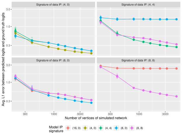
For the first experiment, we consider generating networks with $n$ vertices, where each vertex is given a latent vector $Z_{i}\sim N(0,I_{(p_{+}+p_{-})})$ drawn independently (where $p_{+},p_{-}\in\mathbb{N}$ ), with edges formed between vertices independently with probability

\mathbb{P}(A_{ij}=1|Z_{i},Z_{j})=\sigma\big{(}B_{p_{+},p_{-}}(Z_{i},Z_{j})\big{)}\text{ for }i<j.

Here $\sigma(x)=(1+e^{-x})^{-1}$ is the sigmoid function, and $B_{r,s}(\omega,\omega^{\prime})=\langle\omega,\mathrm{diag}(I_{r},-I_{s})\omega^{\prime}\rangle$ for any $r,s\geq 1$ . We simulate twenty networks for each possible combination of: $n=200$ , $400$ , $800$ , $1200$ , $1600$ , $2400$ , $3200$ , or $4800$ ; and $(p_{+},p_{-})$ equal to $(4,0)$ , $(4,4)$ , $(8,0)$ , or $(8,8)$ . We then train each network using a constant step-size SGD method with a uniform vertex sampler for 40 epochs²²2By epochs, we are referring to the cumulative number of pairs of vertices which are used to form a gradient at each iteration, relative to the total number of edges in the graph., using a similarity measure $B_{q_{+},q_{-}}$ between embedding vectors for various values of $(q_{+},q_{-})$ . Some are equal to $(p_{+},p_{-})$ , so that the similarity measure used for the data generating process and training are identical. Some are greater than $(p_{+},p_{-})$ , so the data generating process still falls within the constraints of the model. Finally, we also let some be less than $(p_{+},p_{-})$ , in which case the data generating process falls outside the specified model class for learning. With the learned embeddings $(\widehat{\omega}_{1},\ldots,\widehat{\omega}_{n})$ we then calculate the value of

\frac{1}{n^{2}}\sum_{i,j\in[n]}\Big{|}B_{q_{+},q_{-}}\big{(}\widehat{\omega}_{i},\widehat{\omega}_{j}\big{)}-B_{p_{+},p_{-}}(Z_{i},Z_{j})\Big{|}.

(27)

In words, we are computing the average $L^{1}$ error between the estimated edge logits using the learned embeddings (with a bilinear form $B_{q_{+},q_{-}}$ between embedding vectors in the loss function), and the actual edge logits used to generate the network. The results are displayed in Figure 1. By the convergence theorems discussed in Sections 3.2 and 3.4, we expect that (27) will be $o_{p}(1)$ if and only if $p_{+}\leq q_{+}$ and $p_{-}\leq q_{-}$ , and indeed this is the trend displayed in Figure 1.

Refer to caption — Figure 1: Simulation results for recovery of latent variables for different similarity measures $B(\omega,\omega^{\prime})$ for generating the network and for learning. The $x$ -axis are the number of vertices, and the $y$ -axis is the calculated value of (27). The results for each of the 20 runs per experiment are displayed translucently, with the average across these simulation runs given in bold.

For the second result, we illustrate the validity of the sampling formulae calculated in Section 4. To do so, we begin by generating a network of $n$ vertices from one of the following stochastic block models, where $\pi$ denotes the community sizes and $P$ the community linkage matrices:

	SBM1:	$\displaystyle\qquad\pi=(1/3,1/3,1/3),\qquad$	$\displaystyle P=\begin{pmatrix}0.7&0.3&0.1\\ 0.3&0.5&0.6\\ 0.1&0.6&0.2\end{pmatrix};$
	SBM2:	$\displaystyle\qquad\pi=(0.1,0.2,0.2,0.3,0.2),\qquad$	$\displaystyle P=\begin{pmatrix}0.75&0.87&0.025&0.81&0.25\\ 0.87&0.93&0.58&0.48&0.45\\ 0.025&0.58&0.68&0.15&0.48\\ 0.81&0.48&0.15&0.80&0.92\\ 0.25&0.45&0.48&0.92&0.62\end{pmatrix}.$

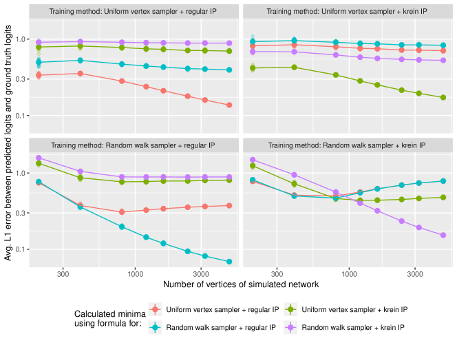
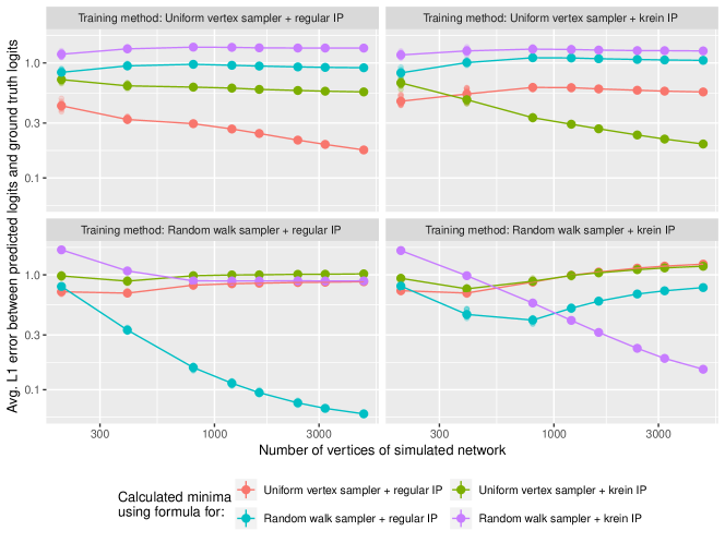
Here each vertex is assigned a latent variable $\lambda_{i}\sim\mathrm{Unif}([0,1])$ which is used to determine the corresponding community (depending on where $\lambda_{i}$ lies within the partition of $[0,1]$ induced by $\pi$ ). As illustrated in Sections 3 and 4, depending on the sampling scheme (samp), and whether we use a regular or Krein inner product (IP) as the similarity measure $B(\omega,\omega^{\prime})$ between embedding vectors (recall Assumption C), there is a function $K^{*}_{\textbf{samp},\textbf{IP}}$ for which the minimizers of (9) satisfy

\frac{1}{n^{2}}\sum_{i,j\in[n]}\Big{|}B(\widehat{\omega}_{i},\widehat{\omega}_{j})-K^{*}_{\textbf{samp},\textbf{IP}}(\lambda_{i},\lambda_{j})\Big{|}=o_{p}(1).

(28)

We note that for stochastic block models, when we choose $B(\omega,\omega^{\prime})=\langle\omega,\omega^{\prime}\rangle$ - corresponding to minimizing $\mathcal{I}_{n}[K]$ over $\mathcal{Z}^{\geq 0}$ - we can numerically compute the formula for $K^{*}_{\textbf{samp},\textbf{IP}}$ via a convex program as a result of Proposition 59. In the case where we choose $B(\omega,\omega^{\prime})$ to be a Krein inner product, the discussion in Section 3.2 tells us that we can write down the minima of $\mathcal{I}_{n}[K]$ over $\mathcal{Z}$ exactly.

For each generated network, we train using either a) a random vertex sampler or a random walk + unigram sampler, and b) either the regular or Krein inner product for $B(\omega,\omega^{\prime})$ . We then calculate the value of (28) for each possible form of $K^{*}_{\textbf{samp},\textbf{IP}}$ for the sampling schemes and inner products we consider. The experiments are then repeated for the same values of $n$ , and number of networks per choice of $n$ , as in the first experiment; the results are displayed in Figure 2. From the figure, we observe that the LHS of (28) decays to zero only when the choice of $K^{*}_{\textbf{samp},\textbf{IP}}$ corresponds to the sampling scheme and inner product actually used, as expected.

5.2 Real data experiments

We now demonstrate on real data sets that the use of the Krein inner product leads to improved prediction of whether vertices are connected in a network, and as a consequence can lead to improvements in downstream tasks performance. To do so, we will consider a semi-supervised multi-label node classification task on two different data sets: a protein-protein interaction network (Grover and Leskovec, 2016; Breitkreutz et al., 2008) with 3,890 vertices, 76,583 edges and 50 classes; and the Blog Catalog data set (Tang and Liu, 2009) with 10,312 vertices, 333,983 edges and 39 classes.

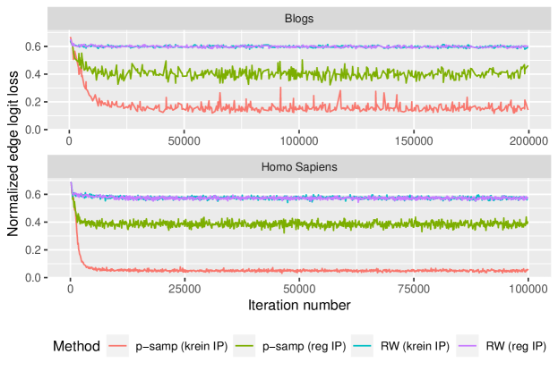
For each data set, we perform the same type of semi-supervised experiments as in Veitch et al. (2018). We learn 128 dimensional embeddings of the networks using two sampling schemes - random walk/skipgram sampling and p-sampling, both augmented with unigram negative samplers - and either a regular inner product (with signature $(128,0)$ ) or a Krein inner product (with signature $(64,64)$ ). We simultaneously train a multinomial logistic regression classifier from the embedding vectors to the vertex classes, with half of the labels censored during training (to be predicted afterwards), and the normalized label loss kept at a ratio of 0.01 to that of the normalized edge logit loss.

After training, we draw test sets according to three different methods (uniform vertex sampling, a random walk sampler and a p-sampler), and calculate the associated macro F1 scores³³3For a multi-class classification problem, the F1 score for a class is the harmonic average of the precision and recall; the macro F1 score is then the arithmetic average of these quantities over all the classes.. The results of this are displayed in Table 1, and the plots of the normalized edge loss during training for each of the data sets can be found in Figure 3. From these, we observe that for each of the data sets when using p-sampling with a unigram negative sampler, there is a large decrease in the normalized edge loss during training when using the Krein inner product compared to the regular inner product. We also see a sizeable increase in the average macro F1 scores. For the skipgram/random walk sampler, we do not observe an improvement in the edge logit loss, but observe a minor increase in macro F1 scores.

Dataset	Sampling scheme	Inner product	Average macro F1 scores
Dataset	Sampling scheme	Inner product	Uniform	Random walk	p-sampling
PPI	Skipgram/RW + NS	Regular	0.203	0.250	0.246
	Skipgram/RW + NS	Krein	0.245	0.298	0.290
	p-sampling + NS	Regular	0.408	0.423	0.417
	p-sampling + NS	Krein	0.486	0.468	0.461
Blogs	Skipgram/RW + NS	Regular	0.154	0.192	0.194
	Skipgram/RW + NS	Krein	0.250	0.279	0.285
	p-sampling + NS	Regular	0.132	0.155	0.166
	p-sampling + NS	Krein	0.349	0.291	0.290

Table 1: Average macro F1 scores for semi-supervised classification for different data sets, sampling schemes, choice of similarity measure

B(\omega,\omega^{\prime})

between embedding vectors, and method of sampling test vertices.

6 Discussion

In our paper, we have obtained convergence guarantees for embeddings learnt via minimizing empirical risks formed through subsampling schemes on a network, in generality for subsampling schemes which depend only on local properties of the network. As a consequence of our theory, we also have argued that using an inner product between embedding vectors in losses of the form (9) can limit the information contained within the learned embedding vectors. Mitigating this through the use of a Krein inner product instead can lead to improved performance in downstream tasks.

We note that our results apply within the framework of (sparsified) exchangeable graphs. While such graphs are convenient for theoretical purposes, and can reflect how real world networks are sparse, they are generally not capable of capturing the power-law type degree distributions of observed networks. There are alternative families of models for network data which are not vertex exchangeable and alleviate some of these problems, such as graphs generated by a graphex process (Veitch and Roy, 2015; Borgs et al., 2017, 2018), along with other models such as those proposed by Caron and Fox (2017) and Crane and Dempsey (2018). As these models all contain enough structure similar to that of exchangeability (such as through an underlying point process to generate the network - see Orbanz (2017) for a general discussion on these points), we anticipate that our overall approach can be used to analyze the performance of embedding methods on broader classes of models for networks.

Our theory only considers embeddings learnt in an unsupervised, transductive fashion, whereas inductive methods for learning network embeddings are increasing popular. We highlight that inductive methods such as GraphSAGE (Hamilton et al., 2017a) work by parameterizing node embeddings through an encoder (possibly with the inclusion of nodal covariates), with the output embeddings then trained through a DeepWalk procedure. Provided that the encoder used is sufficiently flexible so that the range of embedding vectors is unconstrained (which is likely the case for the neural network architectures frequently employed), our results still apply in that we can give convergence guarantees for the output of the encoder analogously to Theorems 10, 12 and 19.

Acknowledgements

We acknowledge computing resources from Columbia University’s Shared Research Computing Facility project, which is supported by NIH Research Facility Improvement Grant 1G20RR030893-01, and associated funds from the New York State Empire State Development, Division of Science Technology and Innovation (NYSTAR) Contract C090171, both awarded April 15, 2010. Part of this work was completed while M. Austern was at Microsoft Research, New England. We thank the two anonymous reviewers and the editor for their feedback, which significantly improved the readability and contributions of the paper.

Appendix A Technical Assumptions

Here we introduce a more general set of technical assumptions than those introduced in Section 2 for which our technical results hold. For convenience, at points we will duplicate our assumptions to keep the labelling consistent, and so Assumptions A,B and E are generalizations of Assumptions 1, 2 and 5 respectively, and Assumptions C and D are the same as Assumptions 3 and 4 respectively.

Assumption A (Regularity and smoothness of the graphon)

We suppose that the underlying sequence of graphons $(W_{n}=\rho_{n}W)_{n\geq 1}$ generating $(\mathcal{G}_{n})_{n\geq 1}$ are, up to weak equivalence of graphons (Lovász, 2012), such that:

a)

The graphon $W$ is piecewise Hölder $([0,1]^{2}$ , $\beta_{W}$ , $L_{W}$ , $\mathcal{Q}^{\otimes 2})$ for some partition $\mathcal{Q}$ of $[0,1]$ and constants $\beta_{W}\in(0,1]$ , $L_{W}\in(0,\infty)$ ;
b)

The degree function $W(x,\cdot)$ is such that $W(x,\cdot)^{-1}\in L^{\gamma_{d}}([0,1])$ for some exponent $\gamma_{d}\in(1,\infty]$ ;
c)

The graphon $W$ is such that $W^{-1}\in L^{\gamma_{W}}([0,1]^{2})$ for some exponent $\gamma_{W}\in[1,\infty]$ ;
d)

There exists a constant $C>0$ such that $1-\rho_{n}W\geq C$ a.e;
e)

The sparsifying sequence $(\rho_{n})_{n\geq 1}$ is such that $\rho_{n}=\omega(n^{-(\gamma_{d}-1)/\gamma_{d}})$ if $\gamma_{d}\in(1,\infty)$ , and $\rho_{n}=\omega(log(n)/n)$ if $\gamma_{d}=\infty$ .

Assumption B (Properties of the loss function)

Assume that the loss function $\ell(y,x)$ is non-negative, twice differentiable and strictly convex in $y\in\mathbb{R}$ for $x\in\{0,1\}$ , and is injective in the sense that if $\ell(y,x)=\ell(\tilde{y},x)$ for $x=0$ and $x=1$ , then $y=\tilde{y}$ . Moreover, we suppose that there exists $p\in[1,\infty)$ (where we call $p$ the growth rate of the loss function $\ell$ ) such that

For $x\in\{0,1\}$ , the loss function $\ell(y,x)$ is locally Lipschitz in that there exists a constant $L_{\ell}$ such that

\big{|}\ell(y,x)-\ell(y^{\prime},x)\big{|}\leq L_{\ell}\max\{|y|,|y^{\prime}|\}^{p-1}|y-y^{\prime}|\text{ for all }y,y^{\prime}\in\mathbb{R};

ii)

Moreover, there exists constants $C_{\ell}>0$ and $a_{\ell}>0$ such that, for all $y\in\mathbb{R}$ and $x\in\{0,1\}$ , we have

\displaystyle\frac{1}{C_{\ell}}(|y|^{p}-a_{\ell})\leq\ell(y,1)+\ell(y,0)\leq C_{\ell}(|y|^{p}+a_{\ell}),\qquad\Big{|}\frac{d}{dy}\ell(y,x)\Big{|}\leq C_{\ell}(|y|^{p-1}+a_{\ell}).

These conditions ensure that $\ell(y,1)$ and $\ell(y,0)$ grows like $|y|^{p}$ as $y\to+\infty$ and $y\to-\infty$ respectively.

Note that the cross-entropy loss satisifies the above conditions with $p=1$ , and also satisifies the conditions below:

Assumption BI (Loss functions arising from probabilistic models)

In addition to requiring all of Assumption B to hold, we additionally suppose that there exists a c.d.f $F$ for which

\ell(y,x)=\ell_{F}(y,x):=-x\log\big{(}F(y)\big{)}-(1-x)\log\big{(}1-F(y)\big{)},

where $F$ corresponds to a distribution which is continuous, symmetric about $0$ , strictly log-concave, and has an inverse which is Lipschitz on compact sets.

In addition to the cross-entropy loss, the above assumptions allows for probit losses (taking $F$ to be the c.d.f of a Gaussian distribution). Note that for such loss functions, the value of $p$ is linked to the tail behavior of the distribution in that it behaves as $\exp(-|y|^{p})$ - for instance, the logistic distribution is sub-exponential and the cross entropy loss satisifies Assumption BI with $p=1$ , whereas a Gaussian is sub-Gaussian and thus Assumption BI will hold with $p=2$ .

Assumption C (Properties of the similarity measure $B(\omega,\omega^{\prime})$ )

Supposing we have embedding vectors $\omega,\omega^{\prime}\in\mathbb{R}^{d}$ , we assume that the similarity measure $B$ is equal to one of the following bilinear forms:

i)

$B(\omega,\omega^{\prime})=\langle\omega,\omega^{\prime}\rangle$ (i.e a regular or definite inner product) or
ii)

$B(\omega,\omega^{\prime})=\langle\omega,I_{d_{1},d-d_{1}}\omega^{\prime}\rangle=\langle\omega_{[1:d_{1}]},\omega^{\prime}_{[1:d_{1}]}\rangle-\langle\omega_{[(d_{1}+1):d]},\omega^{\prime}_{[(d_{1}+1):d]}\rangle$ for some $d_{1}\leq d$ (i.e an indefinite or Krein inner product);

where $I_{p,q}=\mathrm{diag}(I_{p},-I_{q})$ , $\omega_{A}=(\omega_{i})_{i\in A}$ for $A\subseteq[d]$ , and $[a:b]=\{a,a+1,\ldots,b\}$ .

Assumption D (Strong local convergence)

\max_{i,j\in[n],i\neq j}\Big{|}\frac{n^{2}\mathbb{P}((i,j)\in S(\mathcal{G}_{n})|\mathcal{G}_{n})}{f_{n}(\lambda_{i},\lambda_{j},a_{ij})}-1\Big{|}=O_{p}(s_{n})

for some non-negative sequence $s_{n}=o(1)$ .

Assumption E (Regularity of the sampling weighs)

We assume that, for each $n$ , the functions

\tilde{f}_{n}(l,l^{\prime},1):=f_{n}(l,l^{\prime},1)W_{n}(l,l^{\prime})\text{ and }\tilde{f}_{n}(l,l^{\prime},0):=f_{n}(l,l^{\prime},0)(1-W_{n}(l,l^{\prime}))

are piecewise Hölder $([0,1]^{2},\beta,L_{f},\mathcal{Q}^{\otimes 2})$ , where $\mathcal{Q}$ is the same partition as in Assumption Aa), but the exponents $\beta$ and $L_{f}$ may differ from that of $\beta_{W}$ and $L_{W}$ in Assumption Aa). We moreover suppose that $\tilde{f}_{n}(l,l^{\prime},1)$ and $\tilde{f}_{n}(l,l^{\prime},0)$ are uniformly bounded in $L^{\infty}([0,1]^{2})$ , are positive a.e, and that $\tilde{f}_{n}(l,l^{\prime},1)^{-1}$ and $\tilde{f}_{n}(l,l^{\prime},0)^{-1}$ are uniformly bounded in $L^{\gamma_{s}}([0,1]^{2})$ for some constant $\gamma_{s}\in[1,\infty]$ .

Appendix B Proof outline for Theorems 7, 10, 12 and 19

We begin with outlining the approach of the proof of Theorem 7; that is, the convergence of the empirical risk to the population risk. Note that in the expression of the empirical risk $\mathcal{R}_{n}(\bm{\omega}_{n})$ , as a consequence of Assumption 4, we are able to replace the sampling probabilities in $\mathcal{R}_{n}(\bm{\omega}_{n})$ with the $f_{n}(\lambda_{i},\lambda_{j},a_{ij})/n^{2}$ . After also including the terms with $i=j$ , $i\in[n]$ as part of the summation (which is possible as we are adding $O(n)$ terms to an average of $O(n^{2})$ quantities), we can asymptotically consider minimizing the expression

\widehat{\mathcal{R}}_{n}(\omega_{1},\ldots,\omega_{n}):=\frac{1}{n^{2}}\sum_{i,j\in[n]^{2}}f_{n}(\lambda_{i},\lambda_{j},a_{ij})\ell(B(\omega_{i},\omega_{j}),a_{ij}).

To proceed further, we now suppose that $W$ corresponds to a stochastic block model; more specifically, we suppose there exists a partition $\mathcal{Q}=(A_{1},\ldots,A_{\kappa})$ of $[0,1]$ into intervals for which $W(\cdot,\cdot)$ is constant on the $A_{l}\times A_{l^{\prime}}$ for $l,l^{\prime}\in[\kappa(n)]$ . Note that $f_{n}(\cdot,\cdot,x)$ is implicitly a function of $W(\cdot,\cdot)$ for $x\in\{0,1\}$ , and therefore it also piecewise constant on $\mathcal{Q}$ . As an abuse of notation, we write $f_{n}(l,l^{\prime},x)$ for the value of $f_{n}(\lambda_{i},\lambda_{j},x)$ when $(\lambda_{i},\lambda_{j})\in A_{l}\times A_{l^{\prime}}$ . If we write

	$\displaystyle\mathcal{A}_{n}(l)$	$\displaystyle:=\big{\{}i\in[n]\,:\,\lambda_{i}\in A_{l}\big{\}},$
	$\displaystyle\mathcal{A}_{n}(l,l^{\prime})$	$\displaystyle:=\big{\{}i,j\in[n]\,:\,\lambda_{i}\in A_{l},\lambda_{j}\in A_{l^{\prime}}\big{\}}=\mathcal{A}_{n}(l)\times\mathcal{A}_{n}(l^{\prime})$

we can then perform a decomposition of $\widehat{\mathcal{R}}_{n}$ into a sum

	$\displaystyle\widehat{\mathcal{R}}_{n}(\omega_{1},\ldots,\omega_{n})$	$\displaystyle:=\frac{1}{n^{2}}\sum_{l,l^{\prime}\in[\kappa]}\sum_{(i,j)\in\mathcal{A}_{n}(l,l^{\prime})}f_{n}(l,l^{\prime},a_{ij})\ell(B(\omega_{i},\omega_{j}),a_{ij})$
		$\displaystyle=\sum_{l,l^{\prime}\in[\kappa]}\frac{\|\mathcal{A}_{n}(l,l^{\prime})\|}{n^{2}}\cdot\frac{1}{\|\mathcal{A}_{n}(l,l^{\prime})\|}\sum_{(i,j)\in\mathcal{A}_{n}(l,l^{\prime})}f_{n}(l,l^{\prime},a_{ij})\ell(B(\omega_{i},\omega_{j}),a_{ij}).$

For now working conditionally on the $\lambda_{i}$ , we note that for each of the $(l,l^{\prime})$ , the gap between the averages

\frac{1}{|\mathcal{A}_{n}(l,l^{\prime})|}\sum_{(i,j)\in\mathcal{A}_{n}(l,l^{\prime})}f_{n}(l,l^{\prime},a_{ij})\ell(B(\omega_{i},\omega_{j}),a_{ij})

(29)

and

\frac{1}{|\mathcal{A}_{n}(l,l^{\prime})|}\sum_{(i,j)\in\mathcal{A}_{n}(l,l^{\prime})}\big{\{}\tilde{f}_{n}(l,l^{\prime},1)\ell(B(\omega_{i},\omega_{j}),1)+\tilde{f}_{n}(l,l^{\prime},0)\ell(B(\omega_{i},\omega_{j}),0)\big{\}},

(30)

where we recall that $\tilde{f}_{n}(l,l^{\prime},x)=f_{n}(l,l^{\prime},1)W(l,l^{\prime})^{x}[1-W(l,l^{\prime})]^{1-x}$ , will be small asymptotically. In particular, the difference of the two has expectation zero as the expected value of (29) conditional on the $\lambda_{i}$ is (30), and will have variance $O(1/|\mathcal{A}_{n}(l,l^{\prime})|)$ as (29) is an average of $\mathcal{A}_{n}(l,l^{\prime})$ independently distributed bounded random variables. As the variance bound is independent of $\lambda_{i}$ outside of the size of the set $|\mathcal{A}_{n}(l,l^{\prime})|$ , which will be $\Omega_{p}(n^{2})$ , it therefore follows that the difference between (29) and (30) will therefore also be small asymptotically unconditionally on the $\lambda_{i}$ too. We can therefore consider minimizing

\sum_{l,l^{\prime}\in[\kappa]}\frac{|\mathcal{A}_{n}(l,l^{\prime})|}{n^{2}}\cdot\frac{1}{|\mathcal{A}_{n}(l,l^{\prime})|}\sum_{(i,j)\in\mathcal{A}_{n}(l,l^{\prime})}\sum_{x\in\{0,1\}}\tilde{f}_{n}(l,l^{\prime},x)\ell(B(\omega_{i},\omega_{j}),x).

(31)

We now use Jensen’s inequality (which is permissible as the loss is strictly convex) and the bilinearity of $B(\cdot,\cdot)$ , which gives us that

	$\displaystyle\sum_{l,l^{\prime}\in[\kappa]}$	$\displaystyle\frac{\|\mathcal{A}_{n}(l,l^{\prime})\|}{n^{2}}\cdot\frac{1}{\|\mathcal{A}_{n}(l,l^{\prime})\|}\sum_{(i,j)\in\mathcal{A}_{n}(l,l^{\prime})}\sum_{x\in\{0,1\}}\tilde{f}_{n}(l,l^{\prime},x)\ell(B(\omega_{i},\omega_{j}),x)$
		$\displaystyle\geq\sum_{l,l^{\prime}\in[\kappa]}\frac{\|\mathcal{A}_{n}(l,l^{\prime})\|}{n^{2}}\sum_{x\in\{0,1\}}\tilde{f}_{n}(l,l^{\prime},x)\ell\Big{(}B\Big{(}\frac{1}{\|\mathcal{A}_{n}(l)\|}\sum_{i\in\mathcal{A}_{n}(l)}\omega_{i},\frac{1}{\|\mathcal{A}_{n}(l^{\prime})\|}\sum_{j\in\mathcal{A}_{n}(l^{\prime})}\omega_{j}\Big{)},x\Big{)}$
		$\displaystyle=\sum_{l,l^{\prime}\in[\kappa]}\frac{1}{n^{2}}\sum_{(i,j)\in\mathcal{A}_{n}(l,l^{\prime})}\sum_{x\in\{0,1\}}\tilde{f}_{n}(l,l^{\prime},x)\ell(B(\widetilde{\omega}_{i},\widetilde{\omega}_{j}),x)$

where we have defined $\widetilde{\omega}_{i}:=\tfrac{1}{|\mathcal{A}_{n}(l)|}\sum_{j\in\mathcal{A}_{n}(l)}\omega_{j}$ if $i\in\mathcal{A}_{n}(l)$ , and the inequality is strict unless the $B(\omega_{i},\omega_{j})$ are constant across $(i,j)\in\mathcal{A}_{n}(l)\times\mathcal{A}_{n}(l^{\prime})$ . This means that for the purposes of minimizing (31), we know that we can restrict ourselves to only taking an embedding vector $\widetilde{\omega}_{l}$ per latent feature. Making use of the fact that $n^{-2}|\mathcal{A}_{n}(l,l^{\prime})|\stackrel{{\scriptstyle p}}{{\to}}p_{l}p_{l^{\prime}}$ , we are left with

\sum_{l,l^{\prime}\in[\kappa]}p_{l}p_{l^{\prime}}\big{\{}f_{n}(l,l^{\prime},1)W(l,l^{\prime})\ell(B(\widetilde{\omega}_{l},\widetilde{\omega}_{l^{\prime}}),1)+f_{n}(l,l^{\prime},0)[1-W(l,l^{\prime})]\ell(B(\widetilde{\omega}_{l},\widetilde{\omega}_{l^{\prime}}),0)\big{\}}.

Making the identification $\eta(\lambda)=\widetilde{\omega}_{l}$ for $\lambda\in A_{l}$ , we then end up exactly with $\mathcal{I}_{n}[K]$ where $K(l,l^{\prime})=B(\eta(l),\eta(l^{\prime}))$ as desired. The details in the appendix discuss how to apply the argument when $W$ is a general (sufficiently smooth) graphon and not just a stochastic block model, along with arguing that the above functions converge uniformly over the embedding vectors, and not just pointwise.

Once we have the population risk $\mathcal{I}_{n}[K]$ , the proof technique for the convergence of the minimizers to (9) in Theorems 10, 12 and 19 follow the usual strategy for obtaining consistency results - given uniform convergence of an empirical risk to a population risk, we want to show that the latter has a unique minima which is well-separated, in that points which are outside of a neighbourhood of the minima will have function values which are bounded away from the minimal value also. There are a several technical aspects which are handled in the appendix, relating to the infinite dimensional nature of our optimization problem, the non-convexity of the constraint sets $\mathcal{Z}(S_{d})$ and the change in domain from embedding vectors $(\omega_{1},\ldots,\omega_{n})$ to kernels $K(l,l^{\prime})$ .

Appendix C Proof of Theorem 7

For notational convenience, we will write $\bm{\omega}_{n}=(\omega_{1},\ldots,\omega_{n})$ for the collection of embedding vectors for vertices $\{1,\ldots,n\}$ , and write

\sum_{i,j}f(i,j):=\sum_{i,j=1}^{n}f(i,j),\qquad\sum_{i\neq j}f(i,j):=\sum_{i,j\in[n],i\neq j}f(i,j).

We will also write $\bm{\lambda}_{n}:=(\lambda_{1},\ldots,\lambda_{n})$ and $\bm{A}_{n}:=(a_{ij}^{(n)})_{i,j\in[n]}$ for the collection of latent features and adjacency assignments for $\mathcal{G}_{n}$ . We aim to prove the following result:

Theorem 30

Suppose that Assumptions A, B, C, D and E hold. Let $S_{d}=[-A,A]^{d}$ , and write

Z(S_{d}):=\{K:[0,1]^{2}\to\mathbb{R}\,:\,K(l,l^{\prime})=B(\eta(l),\eta(l^{\prime}))\text{ a.e, where }\eta:[0,1]\to S_{d}\}.

Then we have that

\displaystyle\big{|}\min_{\bm{\omega}_{n}\in(S_{d})^{n}}\mathcal{R}_{n}(\bm{\omega}_{n})-\min_{K\in Z(S_{d})}\mathcal{I}_{n}[K]\big{|}=O_{p}\Big{(}s_{n}+\frac{d^{p+1/2}\mathbb{E}[f_{n}^{2}]^{1/2}}{n^{1/2}}+\frac{(\log n)^{1/2}+d^{p/\gamma_{s}}}{n^{\beta/(1+2\beta)}}\Big{)}

where we write $\mathbb{E}[f_{n}^{2}]=\mathbb{E}[f_{n}(\lambda_{1},\lambda_{2},a_{12})^{2}]$ . If moreover we have that $\tilde{f}_{n}(l,l^{\prime},1)$ and $\tilde{f}_{n}(l,l^{\prime},0)$ are piecewise constant functions on a partition $\mathcal{Q}^{\otimes 2}$ where $\mathcal{Q}$ is of size $\kappa$ , then

\displaystyle\big{|}\min_{\bm{\omega}_{n}\in(S_{d})^{n}}\mathcal{R}_{n}(\bm{\omega}_{n})-\min_{K\in Z(S_{d})}\mathcal{I}_{n}[K]\big{|}=O_{p}\Big{(}s_{n}+\frac{d^{p+1/2}\mathbb{E}[f_{n}^{2}]^{1/2}}{n^{1/2}}+\frac{(\log\kappa)^{1/2}}{n^{1/2}}\Big{)}.

Remark 31 (Issues of measurability)

We make one technical point at the beginning of the proof to prevent repetition - throughout we will be taking infima and suprema of uncountably many random variables over sets which depend on the $\bm{\lambda}_{n}$ and $\bm{A}_{n}$ . Moreover, we will want to reason about either these minimal/maximal values, or the corresponding argmin sets. We need to ensure the measurability of these types of quantities.

We note two important facts which will allow us to do so: the fact that the $f_{n}(\lambda_{i},\lambda_{j},a_{ij})$ are measurable functions, and that the loss functions $\ell(\cdot,x)$ are continuous for $x\in\{0,1\}$ . Consequently, all of the functions we take suprema or minima over are Carathédory; that is of the form $g:X\times S\to\mathbb{R}$ , where $x\mapsto g(x,s)$ is continuous for all $s\in S$ , and $s\mapsto g(x,s)$ is measurable for all $x\in X$ . Here $X$ plays the role of some Euclidean space, and $S$ a probability space supporting the $\bm{\lambda}_{n}$ and $\bm{A}_{n}$ . Moreover, all of our suprema and minima will be taken either over a) a non-random compact subset $K$ of $\mathbb{R}^{m}$ for some $m$ , or b) a set of the form

\displaystyle\phi(s)

\displaystyle:=\{x\in K(s)\,:\,g(x,s)\leq Cg(0,s)\}

where i) $K(s):=\{\bm{x}\in\mathbb{R}^{m}\,:\,\|x\|\leq f(s)\}$ for some measurable function $f(s)$ and norm $\|x\|$ on $\mathbb{R}^{m}$ , ii) $g(x,s)$ is Carathédory, and iii) the constant $C$ satisfies $C>1$ (so $\phi(s)$ is non-empty). With this, we can guarantee the measurability of any quantities we will consider; an application of Aubin and Frankowska (2009, Theorem 8.2.9) implies that $K(s)$ , and therefore also $\phi(s)$ , are measurable correspondences with non-empty compact values, and therefore the measurable maximum theorem (e.g Aliprantis and Border, 2006, Theorem 18.19) will guarantee the measurability of all the quantities we want to consider.

C.1 Replacing sampling probabilities with $f_{n}(\lambda_{i},\lambda_{j},a_{ij})/n^{2}$

To begin, we justify why minimizing

\widehat{\mathcal{R}}_{n}(\bm{\omega}_{n}):=\frac{1}{n^{2}}\sum_{i\neq j}f_{n}(\lambda_{i},\lambda_{j},a_{ij})\ell(B(\omega_{i},\omega_{j}),a_{ij})

is asymptotically equivalent to that of minimizing $\mathcal{R}_{n}(\bm{\omega}_{n})$ .

Lemma 32

Assume that Assumptions B and D hold. Then there exists a non-empty random measurable set $\Psi_{n}$ such that

\mathbb{P}\Big{(}\operatorname*{arg\,min}_{\bm{\omega}_{n}\in(S_{d})^{n}}\mathcal{R}_{n}(\bm{\omega}_{n})\cup\operatorname*{arg\,min}_{\bm{\omega}_{n}\in(S_{d})^{n}}\widehat{\mathcal{R}}_{n}(\bm{\omega}_{n})\subseteq\Psi_{n}\Big{)}\to 1,\quad\sup_{\bm{\omega}_{n}\in\Psi_{n}}\Big{|}\mathcal{R}_{n}(\bm{\omega}_{n})-\widehat{\mathcal{R}}_{n}(\bm{\omega}_{n})\Big{|}=O_{p}(s_{n}).

Proof [Proof of Lemma 32] We will argue that the loss functions will converge uniformly over sets of the form $\mathcal{R}_{n}(\bm{\omega}_{n})\leq C\mathcal{R}_{n}(\bm{0})$ , where $C$ can be any constant strictly greater than one. Such sets contain the minima of e.g $\mathcal{R}_{n}(\bm{\omega}_{n})$ , and as we are working on (stochastically) bounded level sets of $\mathcal{R}_{n}(\bm{\omega}_{n})$ , this will be enough to allow us to use Assumption D in order to obtain the desired conclusion. With this in mind, we denote $C_{\ell,0}=\max_{x\in\{0,1\}}\ell(0,x)$ and then define the sets

	$\displaystyle\Psi_{n}$	$\displaystyle:=\Bigg{\{}\bm{\omega}_{n}\in(S_{d})^{n}\,:\,\mathcal{R}_{n}(\bm{\omega}_{n})\leq 2C_{\ell,0}\sum_{i\neq j}\mathbb{P}((i,j)\in S(\mathcal{G}_{n})\|\mathcal{G}_{n})\Bigg{\}},$
	$\displaystyle\widehat{\Psi}_{n}$	$\displaystyle:=\Bigg{\{}\bm{\omega}_{n}\in(S_{d})^{n}\,:\,\widehat{\mathcal{R}}_{n}(\bm{\omega}_{n})\leq C_{\ell,0}\sum_{i\neq j}\frac{f_{n}(\lambda_{i},\lambda_{j},a_{ij})}{n^{2}}\Bigg{\}}.$

Our aim is to show that $\widehat{\Psi}_{n}\subseteq\Psi_{n}$ with asymptotic probability $1$ . Note that

\mathcal{R}_{n}(\bm{0})\leq C_{\ell,0}\sum_{i\neq j}\mathbb{P}((i,j)\in S(\mathcal{G}_{n})|\mathcal{G}_{n}),\qquad\widehat{\mathcal{R}}_{n}(\bm{0})\leq C_{\ell,0}\sum_{i\neq j}\frac{f_{n}(\lambda_{i},\lambda_{j},a_{ij})}{n^{2}}

so $\bm{0}\in\Psi_{n}$ and $\bm{0}\in\widehat{\Psi}_{n}$ (meaning the sets are non-empty). Moreover, these sets will always contain the argmin sets of $\mathcal{R}_{n}(\bm{\omega}_{n})$ and $\widehat{\mathcal{R}}_{n}(\bm{\omega}_{n})$ respectively (as any minimizer $\bm{\omega}_{n}$ will satisfy e.g $\mathcal{R}_{n}(\bm{\omega}_{n})\leq\mathcal{R}_{n}(\bm{0})$ ). In particular, once we show that $\mathbb{P}(\widehat{\Psi}_{n}\subseteq\Psi_{n})\to 1$ as $n\to\infty$ , we will have shown the first part of the lemma, and we can then reduce to showing uniform convergence of $\mathcal{R}_{n}(\bm{\omega}_{n})-\widehat{\mathcal{R}}_{n}(\bm{\omega}_{n})$ over $\Psi_{n}$ . Pick an arbitrary $\bm{\omega}_{n}\in\widehat{\Psi}_{n}$ . Then by Assumption D, we get that

	$\displaystyle\mathcal{R}_{n}(\bm{\omega}_{n})$	$\displaystyle=\sum_{i\neq j}\frac{n^{2}\mathbb{P}((i,j)\in S(\mathcal{G}_{n})\|\mathcal{G}_{n})}{f_{n}(\lambda_{i},\lambda_{j},a_{ij})}\frac{f_{n}(\lambda_{i},\lambda_{j},a_{ij})}{n^{2}}\ell(B(\omega_{i},\omega_{j}),a_{ij})$
		$\displaystyle\leq\sup_{i\neq j}\frac{n^{2}\mathbb{P}((i,j)\in S(\mathcal{G}_{n})\|\mathcal{G}_{n})}{f_{n}(\lambda_{i},\lambda_{j},a_{ij})}\cdot\widehat{\mathcal{R}}_{n}(\bm{\omega}_{n})\leq C_{\ell,0}(1+o_{p}(1))\sum_{i\neq j}\frac{f_{n}(\lambda_{i},\lambda_{j},a_{ij})}{n^{2}}.$

By Lemma 48 - noting that with asymptotic probability $1$ all the quantities involved are positive - we have that

\frac{\sum_{i\neq j}n^{-2}f_{n}(\lambda_{i},\lambda_{j},a_{ij})}{\sum_{i\neq j}\mathbb{P}((i,j)\in S(\mathcal{G}_{n})|\mathcal{G}_{n})}\leq\sup_{i\neq j}\frac{f_{n}(\lambda_{i},\lambda_{j},a_{ij})}{n^{2}\mathbb{P}((i,j)\in S(\mathcal{G}_{n})|\mathcal{G}_{n})}=1+o_{p}(1)

(32)

and so

\mathcal{R}_{n}(\bm{\omega}_{n})\leq C_{\ell,0}(1+o_{p}(1))^{2}\sum_{i\neq j}\mathbb{P}((i,j)\in S(\mathcal{G}_{n})|\mathcal{G}_{n})\stackrel{{\scriptstyle\text{w.h.p}}}{{\leq}}2C_{\ell,0}\sum_{i\neq j}\mathbb{P}((i,j)\in S(\mathcal{G}_{n})|\mathcal{G}_{n})

for $n$ sufficiently large. This holds freely of the choice of $\bm{\omega}_{n}\in\widehat{\Psi}_{n}$ , and so $\widehat{\Psi}_{n}\subseteq\Psi_{n}$ with asymptotic probability $1$ . To conclude, we then note that over the set $\Psi_{n}$ , we have

	$\displaystyle\sup_{\bm{\omega}_{n}\in\Psi_{n}}$	$\displaystyle\Big{\|}\sum_{i\neq j}\Big{[}\mathbb{P}((i,j)\in S(\mathcal{G}_{n})\|\mathcal{G}_{n})-\frac{f_{n}(\lambda_{i},\lambda_{j},a_{ij})}{n^{2}}\Big{]}\ell(B(\omega_{i},\omega_{j}),a_{ij})\Big{\|}$
		$\displaystyle\leq\sup_{i\neq j}\Big{\|}\frac{n^{2}\mathbb{P}((i,j)\in S(\mathcal{G}_{n})\|\mathcal{G}_{n})}{f_{n}(\lambda_{i},\lambda_{j},a_{ij})}-1\Big{\|}\cdot\sup_{\bm{\omega}_{n}\in\Psi_{n}}\mathcal{R}_{n}(\bm{\omega}_{n})\leq O_{p}(s_{n})\cdot\mathcal{R}_{n}(\bm{0})=O_{p}(s_{n})$

as desired. Here we use the fact that $\mathcal{R}_{n}(\bm{0})$ is $O_{p}(1)$ , which follows as a result of the fact that $\sum_{i\neq j}f_{n}(\lambda_{i},\lambda_{j},a_{ij})n^{-2}$ is $O_{p}(1)$ by Lemma 49 and $\sup_{n\geq 1}\mathbb{E}[f_{n}(\lambda_{i},\lambda_{j},a_{ij})]<\infty$ (by Assumption D), and then noting that

\sum_{i\neq j}\mathbb{P}\big{(}(i,j)\in S(\mathcal{G}_{n})\,|\,\mathcal{G}_{n}\big{)}=(1+o_{p}(1))\frac{1}{n^{2}}\sum_{i\neq j}f_{n}(\lambda_{i},\lambda_{j},a_{ij})

analogously to (32).

C.2 Averaging the empirical loss over possible edge assignments

Now that we can work with $\widehat{\mathcal{R}}_{n}(\bm{\omega}_{n})$ , we want to examine what occurs as we take $n\to\infty$ . Intuitively, what we will attain should correspond to what occurs when we average this risk over the sampling distribution of the graph; to do so, we begin by averaging over the $a_{ij}$ (while working conditionally on the $\lambda_{i}$ ). As a result, we want to argue that $\widehat{\mathcal{R}}_{n}(\bm{\omega}_{n})$ is asymptotically close to

\mathbb{E}[\widehat{\mathcal{R}}_{n}(\bm{\omega}_{n})|\bm{\lambda}_{n}]:=\frac{1}{n^{2}}\sum_{i\neq j}\sum_{x\in\{0,1\}}\tilde{f}_{n}(\lambda_{i},\lambda_{j},x)\ell(B(\omega_{i},\omega_{j}),x),

(33)

where we recall

\tilde{f}_{n}(\lambda_{i},\lambda_{j},1)=f_{n}(\lambda_{i},\lambda_{j},1)W_{n}(\lambda_{i},\lambda_{j}),\qquad\tilde{f}_{n}(\lambda_{i},\lambda_{j},0)=f_{n}(\lambda_{i},\lambda_{j},0)[1-W_{n}(\lambda_{i},\lambda_{j})].

As the above functions depend only on the values of the $B(\omega_{i},\omega_{j})=:\Omega_{ij}$ , we will freely interchange between the functions having argument $\Omega$ or $\bm{\omega}_{n}$ (whichever is most convenient, mostly for the sake of saving space), with the dependence of $\Omega$ on $\bm{\omega}_{n}$ implicit. We write

Z_{n}(S_{d}):=\{\Omega\in\mathbb{R}^{n\times n}\,:\,\Omega_{ij}=B(\omega_{i},\omega_{j}),\,\omega_{i}\in S_{d}\text{ for }i\in[n]\}

(34)

for the corresponding set of $\Omega$ which are induced via $\bm{\omega}_{n}\in(S_{d})^{n}$ , and define the metric

s_{\ell,\infty}\big{(}\Omega,\widetilde{\Omega}\big{)}:=\max_{i,j\in[n]}\max\big{\{}|\ell(\Omega_{ij},1)-\ell(\widetilde{\Omega}_{ij},1)|,|\ell(\Omega_{ij},0)-\ell(\widetilde{\Omega}_{ij},0)|\big{\}},

(35)

which is induced by the choice of loss function $\ell(y,x)$ in Assumption B. (The injectivity constraints on the loss function specified in Assumption B ensure that $s_{\ell,\infty}(\Omega,\widetilde{\Omega})=0\iff\Omega=\widetilde{\Omega}$ ; the remaining metric properties follow immediately.) We now work towards proving the following result:

Theorem 33

Suppose that Assumptions B and D hold. Then we have that

\sup_{\Omega\in Z_{n}(S_{d})}\big{|}\mathbb{E}[\widehat{\mathcal{R}}_{n}(\Omega)\,|\,\bm{\lambda}_{n}]-\widehat{\mathcal{R}}_{n}(\Omega)\big{|}=O_{p}\Big{(}\frac{\gamma_{2}(Z_{n}(S_{d}),s_{\ell,\infty})\mathbb{E}[f_{n}(\lambda_{1},\lambda_{2},a_{12})^{2}]^{1/2}}{n}\Big{)}

where $\gamma_{2}(T,s)$ denotes the Talagrand $\gamma_{2}$ -functional of a metric space $(T,s)$ .

Here the Talagrand $\gamma_{2}$ -functional is defined as

\gamma_{2}(T,s):=\inf\sup_{t\in T}\sum_{n\geq 0}2^{n/2}\Delta(A_{n}(t),s)

where the infimum is taken over all refining sequences $(\mathcal{A}_{n})_{n\geq 1}$ of partitions of $T$ , where $|\mathcal{A}_{n}|\leq 2^{2^{n}}$ for $n\geq 1$ and $|\mathcal{A}_{0}|=1$ , $A_{n}(t)$ denotes the unique partition of $\mathcal{A}_{n}$ for which $t$ lies within the partition, and $\Delta(T,s):=\sup_{t,v\in T}s(t,v)$ denotes the diameter of $(T,s)$ . See Talagrand (2014, Chapter 2) for various definitions which are equivalent up to universal constants.

Remark 34

We briefly note that rather than calculating the above quantity explicitly, all we require⁴⁴4We note that when $T\subseteq\mathbb{R}^{m}$ , $\gamma_{2}(T,s)$ can only be smaller than the metric entropy by a factor of $\log(m)$ (Talagrand, 2014, Exercise 2.3.4), and so this bound will be tight enough for our purposes. are the bounds

\Delta(T,s)\leq\gamma_{2}(T,s)\leq C\int_{0}^{\infty}\sqrt{\log N(T,s,\epsilon)}\,d\epsilon,

where $C$ is some universal constant, and $N(T,s,\epsilon)$ is the minimal size of an $\epsilon$ -covering of $T$ with respect to the metric $s$ (so the RHS is simply the metric entropy of $(T,s)$ ). We state the bound in terms of $\gamma_{2}(T,s)$ simply as it allows for the easier use of the chaining bound (Theorem 35) stated and used later.

The proof technique consists of a combination of a truncation argument, a chaining argument, and the method of exchangeable pairs. To recap from Chatterjee (2005) the method of exchangeable pairs, suppose that $X$ is a random variable on a Banach space and $f$ is a measurable function such that $\mathbb{E}[f(X)]=0$ . Given an exchangeable pair $(X,X^{\prime})$ (so that $(X,X^{\prime})=(X^{\prime},X)$ in distribution) and an anti-symmetric function $F(X,X^{\prime})$ such that

\mathbb{E}[F(X,X^{\prime})\,|\,X]=f(X),

then provided one has $\mathbb{E}[e^{\theta f(X)}|F(X,X^{\prime})|]<\infty$ and the “variance bound”

v(X):=\frac{1}{2}\mathbb{E}\big{[}|\{f(X)-f(X^{\prime})\}F(X,X^{\prime})|\,\big{|}\,X\big{]}\leq C

(36)

almost surely for some constant $C>0$ , then we have a concentration inequality for the tails of $f(X)$ of the form

\mathbb{P}\big{(}|f(X)|>\eta\big{)}\leq 2e^{-\eta^{2}/2C}\text{ for all }\eta>0.

In particular, we can interpret this as saying that $f(X)$ is sub-Gaussian. If we now had a mean zero stochastic process $\{f_{t}(X)\}_{t\in T}$ where we equip $T$ with a metric $s(\cdot,\cdot)$ , and we could also construct an exchangeable pair $(X,X^{\prime})$ and functions $F_{t,v}(X,X^{\prime})$ for $t,v\in T$ such that i) $\mathbb{E}[F_{t,v}(X,X^{\prime})|X]=f_{t}(X)-f_{v}(X)$ and ii) the corresponding variance term (36) is bounded by $Cs(t,v)^{2}$ , we have the tail bound

\mathbb{P}\Big{(}|f_{t}(X)-f_{v}(X)|>\eta s(t,v)\Big{)}\leq 2e^{-\eta^{2}/2C}\text{ for all }\eta>0.

We could then apply standard chaining results for the supremum of sub-Gaussian processes, such as those in Talagrand (2014):

Proposition 35 (Talagrand, 2014, Theorem 2.2.27)

Let $(T,s)$ be a metric space and suppose $(X_{t})_{t\in T}$ is a mean-zero stochastic process on $(T,s)$ . Suppose that there exists a constant $\sigma>0$ such that for all $t,v\in T$ ,

\mathbb{P}\big{(}|X_{t}-X_{v}|>\eta s(t,v)\big{)}\leq 2e^{-\eta^{2}/2\sigma^{2}}\text{ for all }\eta>0.

Then there exist universal constants $L>0$ and $L^{\prime}>0$ such that

\mathbb{P}\Big{(}\sup_{t,v\in T}|X_{t}-X_{v}|>\sigma L\big{(}\gamma_{2}(T,s)+\eta\Delta(T,s)\big{)}\Big{)}\leq L^{\prime}e^{-\eta^{2}}

for all $\eta>0$ , where $\gamma_{2}(T,s)$ is the Talagrand $\gamma_{2}$ -functional of $(T,s)$ and $\Delta(T,s)$ denotes the diameter of the set $T$ with respect to $s$ .

In particular, this result allows one to easily control the supremum of a stochastic process with an uncountable index, by exploiting the continuity of the underlying process. With the above result, we can rephrase Theorem 33 in terms of controlling the supremum of the absolute value of the stochastic process

	$\displaystyle E_{n}(\Omega)[\bm{A}_{n}]$	$\displaystyle:=\widehat{\mathcal{R}}_{n}(\Omega)-\mathbb{E}[\widehat{\mathcal{R}}_{n}(\Omega)\,\|\,\bm{\lambda}_{n}]$		(37)
		$\displaystyle=\frac{1}{n^{2}}\sum_{i\neq j}f_{n}(\lambda_{i},\lambda_{j},a_{ij})\ell(\Omega_{ij},a_{ij})-\frac{1}{n^{2}}\sum_{i\neq j}\sum_{x\in\{0,1\}}\tilde{f}_{n}(\lambda_{i},\lambda_{j},x)\ell(\Omega_{ij},x)$

over $\Omega\in Z_{n}(S_{d})$ , where we keep track of $\bm{A}_{n}$ where necessary (and will suppress the dependence on this when not). To control the above stochastic process, we will use the method of exchangeable pairs, while working conditional on the $\bm{\lambda}_{n}$ , to give us control of (37) for fixed $\Omega$ ; we can then use Proposition 35 to give us control over all the $\Omega\in Z_{n}(S_{d})$ . We note that as our argument will partly employ a truncation argument, we require the following minor modification of the method of exchangeable pairs:

Lemma 36

Suppose that $X$ is an exchangeable pair with functions $f(X)$ and $F(X,X^{\prime})$ satisfying the conditions stated above, and moreover that $B\in\sigma(X)$ is an event such that $B\subseteq\{v(X)\leq C\}$ and $\mathbb{E}[e^{\theta f(X)}|F(X,X^{\prime})|1_{B}]<\infty$ for all $\theta$ . Then

\mathbb{P}\big{(}|f(X)|>t,B\big{)}\leq 2e^{-t^{2}/2C}\text{ for all }t>0.

Proof [Proof of Lemma 36] The method of proof is identical to that of (Chatterjee, 2005), except one replaces the moment generating function of $f(X)$ with $m(\theta):=\mathbb{E}[e^{\theta f(X)}1_{B}]$ . Following the proof through gives $|m^{\prime}(\theta)|\leq C|\theta|m(\theta)$ , and so $m(\theta)\leq e^{C\theta^{2}/2}$ , and so the result follows from optimizing the Chernoff bound

	$\displaystyle\mathbb{P}\big{(}f(X)>t,B\big{)}$	$\displaystyle\leq\mathbb{P}\big{(}e^{\theta f(X)}>e^{\theta t},B\big{)}=\mathbb{E}\big{[}1[e^{\theta f(X)}>e^{\theta t}]1_{B}\big{]}$
		$\displaystyle\leq e^{-\theta t}\mathbb{E}[e^{\theta f(X)}1_{B}]\leq e^{-\theta t+C\theta^{2}/2}$

with $\theta=t/C$ as usual (and similarly so for the reverse tail).

Proof [Proof of Theorem 33] (Step 1: Breaking up the tail bound into controllable terms.) To begin, we define

$\displaystyle C_{n,1}(\bm{\lambda}_{n},\bm{A}_{n})$	$\displaystyle:=\frac{1}{n^{2}}\sum_{i\neq j}f_{n}(\lambda_{i},\lambda_{j},a_{ij})^{2},$	(38)
$\displaystyle C_{n,2}(\bm{\lambda}_{n})$	$\displaystyle:=\frac{1}{n^{2}}\sum_{i\neq j}\mathbb{E}\big{[}f_{n}(\lambda_{i},\lambda_{j},a_{ij})^{2}\,\|\,\bm{\lambda}_{n}\big{]}$
	$\displaystyle=\frac{1}{n^{2}}\sum_{i\neq j}\big{\{}f_{n}(\lambda_{i},\lambda_{j},1)^{2}W_{n}(\lambda_{i},\lambda_{j})+f_{n}(\lambda_{i},\lambda_{j},0)^{2}(1-W_{n}(\lambda_{i},\lambda_{j}))\big{\}}$	(39)

and note that $\mathbb{E}[C_{n,1}(\bm{A}_{n},\bm{\lambda}_{n})\,|\,\bm{\lambda}_{n}]=C_{n,2}(\bm{\lambda}_{n})$ . We now fix $\epsilon>0$ . By Lemma 49 we know that $C_{n,2}=O_{p}(\mathbb{E}[f_{n}^{2}])$ (where we understand that $\mathbb{E}[f_{n}^{2}]=\mathbb{E}[f_{n}(\lambda_{1},\lambda_{2},a_{12})^{2}]$ ), and therefore there exists $N(\epsilon),M_{2}(\epsilon)$ for which, once $n\geq N(\epsilon)$ , we have that

\mathbb{P}(C_{n,2}(\bm{\lambda}_{n})\geq\mathbb{E}[f_{n}^{2}]M_{2})\leq\frac{\epsilon}{4}.

As by Markov’s inequality we have that

\mathbb{P}\big{(}C_{n,1}(\bm{A}_{n},\bm{\lambda}_{n})>t\,|\,\bm{\lambda}_{n}\big{)}\leq\frac{C_{n,2}(\bm{\lambda}_{n})}{t}\qquad\text{ a.s }

for any $t>0$ , if we define $B_{n,2}:=\{C_{n,2}(\bm{\lambda}_{n})\leq\mathbb{E}[f_{n}^{2}]M_{2}\}$ we therefore have that for $n\geq N(\epsilon)$ that

\mathbb{P}\big{(}C_{n,1}(\bm{A}_{n},\bm{\lambda}_{n})>t\mathbb{E}[f_{n}^{2}]M_{2}\,|\,\bm{\lambda}_{n}\big{)}1_{B_{n,2}}\leq\frac{1}{t}\frac{C_{n,2}(\bm{\lambda}_{n})}{\mathbb{E}[f_{n}^{2}]M_{2}}1_{B_{n,2}}\leq\frac{1}{t}\qquad\text{ a.s }

and therefore there exists $M_{1}(\epsilon)$ such that, once $n\geq N(\epsilon)$ , we have that

\mathbb{E}\Big{[}\mathbb{P}\big{(}C_{n,1}(\bm{A}_{n},\bm{\lambda}_{n})>M_{1}M_{2}\mathbb{E}[f_{n}^{2}]\,|\,\bm{\lambda}_{n}\big{)}1_{B_{n,2}}\Big{]}\leq\frac{\epsilon}{4}.

Writing $B_{n,1}:=\{C_{n,1}(\bm{A}_{n},\bm{\lambda}_{n})\leq\mathbb{E}[f_{n}^{2}]M_{1}M_{2}\}$ , we now write

	$\displaystyle\mathbb{P}\Big{(}\sup_{\Omega\in Z_{n}(S_{d})}$	$\displaystyle\|E_{n}[\Omega]\|>\eta\Big{)}\leq\mathbb{P}\Big{(}\sup_{\Omega\in Z_{n}(S_{d})}\|E_{n}[\Omega]\|>\eta,B_{n,2}\Big{)}+\mathbb{P}(B_{n,2}^{c})$
		$\displaystyle\leq\mathbb{E}\Bigg{[}\mathbb{P}\Big{(}\sup_{\Omega\in Z_{n}(S_{d})}\|E_{n}[\Omega]\|>\eta,B_{n,1}\,\|\,\bm{\lambda}_{n}\Big{)}1_{B_{n,2}}\Bigg{]}+\mathbb{E}\big{[}\mathbb{P}(B_{n,1}^{c}\,\|\,\bm{\lambda}_{n})1_{B_{n,2}}\big{]}+\mathbb{P}(B_{n,2}^{c})$
		$\displaystyle\leq\mathbb{E}\Bigg{[}\mathbb{P}\Big{(}\sup_{\Omega\in Z_{n}(S_{d})}\|E_{n}[\Omega]-E_{n}[0]\|>\eta/2,B_{n,1}\,\|\,\bm{\lambda}_{n}\Big{)}1_{B_{n,2}}\Bigg{]}$
		$\displaystyle\qquad+\mathbb{E}\Bigg{[}\mathbb{P}\Big{(}\|E_{n}[0]\|>\eta/2,B_{n,1}\,\|\,\bm{\lambda}_{n}\Big{)}1_{B_{n,2}}\Bigg{]}+\mathbb{E}\big{[}\mathbb{P}(B_{n,1}^{c}\,\|\,\bm{\lambda}_{n})1_{B_{n,2}}\big{]}+\mathbb{P}(B_{n,2}^{c})$
		$\displaystyle:=(\mathrm{I})+(\mathrm{II})+(\mathrm{III})+(\mathrm{IV})$

and control each of the four terms. For the latter two terms $(\mathrm{III})$ and $(\mathrm{IV})$ , we know that once $n\geq N(\epsilon)$ , their sum is less than or equal to $\epsilon/2$ , and so we focus on the details for the first two terms. For the first term, we will show that for any $\Omega,\widetilde{\Omega}\in Z_{n}(S_{d})$ that

\mathbb{P}\Big{(}\big{|}E_{n}[\Omega]-E_{n}[\widetilde{\Omega}]\big{|}>\eta,B_{n,1}\,|\,\bm{\lambda}_{n}\Big{)}1_{B_{n,2}}\leq 2\exp\Big{(}-\frac{\eta^{2}}{2\mathbb{E}[f_{n}^{2}]M_{2}(1+M_{1})n^{-2}s_{\ell,\infty}\big{(}\Omega,\widetilde{\Omega}\big{)}^{2}}\Big{)}

(40)

which allows us to apply Proposition 35, and for the second term we will get that

\mathbb{P}\big{(}|E_{n}[0]|>\eta,B_{n,1}\,|\,\bm{\lambda}_{n}\big{)}1_{B_{n,2}}\leq 2\exp\Big{(}-\frac{\eta^{2}}{2\mathbb{E}[f_{n}^{2}]M_{2}(1+M_{1})C_{\ell,0}^{2}n^{-2}}\Big{)}

(41)

where $C_{\ell,0}=\max_{x\in\{0,1\}}\ell(0,x)$ . As the details are essentially identical for both, we will through the proof of (40) only. Before doing so though, we show how these results will allow us to obtain the theorem statement. Note that as a consequence of Proposition 35 (recall that $L,L^{\prime}$ are universal constants introduced in the chaining bound) we have, writing $M_{3}:=C_{M}L\sqrt{2M_{2}(1+M_{1})}$ (where $C_{M}\geq 1$ is a constant we choose later) and $\widetilde{\eta}\geq(\log(4L^{\prime}/\epsilon))^{1/2}$ , that

$\displaystyle\mathbb{P}$	$\displaystyle\Big{(}\sup_{\Omega\in Z_{n}(S_{d})}\|E_{n}[\Omega]-E_{n}[0]\|>\tfrac{M_{3}\mathbb{E}[f_{n}^{2}]^{1/2}}{n}\big{[}\gamma_{2}(Z_{n}(S_{d}))+\widetilde{\eta}\Delta(Z_{n}(S_{d}))\big{]},B_{n,1}\,\|\,\bm{\lambda}_{n}\Big{)}1_{B_{n,2}}$	(42)
	$\displaystyle\leq\mathbb{P}\Big{(}\sup_{\Omega,\widetilde{\Omega}\in Z_{n}(S_{d})}\|E_{n}[\Omega]-E_{n}[\widetilde{\Omega}]\|>\tfrac{M_{3}\mathbb{E}[f_{n}^{2}]^{1/2}}{n}\big{[}\gamma_{2}(Z_{n}(S_{d}))+\widetilde{\eta}\Delta(Z_{n}(S_{d}))\big{]},B_{n,1}\,\|\,\bm{\lambda}_{n}\Big{)}1_{B_{n,2}}$
	$\displaystyle\leq L^{\prime}e^{-\widetilde{\eta}^{2}}\leq\epsilon/4.$

Here we have temporarily suppressed the dependence of the metric on $\gamma_{2}(T,s)$ and $\Delta(T,s)$ for reasons of space, and note that the above inequality holds provided $C_{M}\geq 1$ . Taking expectations then allows us to show that $(\mathrm{I})\leq\epsilon/4$ by taking any

\eta\geq M_{3}\Big{(}\frac{\gamma_{2}(Z_{n}(S_{d}),s_{\ell,\infty})\mathbb{E}[f_{n}^{2}]^{1/2}}{n}+\sqrt{\log\Big{(}\frac{4L^{\prime}}{\epsilon}\Big{)}}\frac{\Delta(Z_{n}(S_{d}),s_{\ell,\infty})\mathbb{E}[f_{n}^{2}]^{1/2}}{n}\Big{)}

(where we have inverted the bound in (42) and substituted in the value of $\tilde{\eta}$ ). By using such a choice of $\eta$ , we then note that in (41) we get that

	$\displaystyle\mathbb{P}\big{(}\|E_{n}[0]\|$	$\displaystyle>\eta,B_{n,1}\,\|\,\bm{\lambda}_{n}\big{)}1_{B_{n,2}}$
		$\displaystyle\leq 2\exp\Big{(}-C_{M}^{2}L^{2}C_{\ell,0}^{-2}\{\gamma_{2}(Z_{n}(S_{d}),s_{\ell,\infty})+\tilde{\eta}\Delta(Z_{n}(S_{d}),s_{\ell,\infty})\}/4\Big{)}.$

Noting that $A^{2}d\leq\Delta(Z_{n}(S_{d}),s_{\ell,\infty})\leq\gamma_{2}(Z_{n}(S_{d}),s_{\ell,\infty})$ (recall Remark 34), it therefore follows that by choosing

C_{M}=\max\{1,C_{\ell,0}A^{-1}L^{-1}d^{-1/2}\sqrt{\log(8/\epsilon)}\}

in the expression for $M_{3}$ , we get that $(\mathrm{II})\leq\epsilon/4$ also.

Putting this altogether, as we have that $\gamma_{2}(Z_{n}(S_{d}),s_{\ell,\infty})\geq\Delta(Z_{n}(S_{d}),s_{\ell,\infty})$ , it therefore follows from the above discussion that given any $\epsilon>0$ , we will be able to find constants $N(\epsilon)$ and $M(\epsilon)$ (the value of $N$ given at the beginning of the proof; for $M$ , the value of $M_{3}(1+\tilde{\eta})$ from the discussion above), such that once $n\geq N(\epsilon)$ , we have that

\mathbb{P}\Big{(}\sup_{\Omega\in Z_{n}(S_{d})}|E_{n}(\Omega)|>M\frac{\gamma_{2}(Z_{n}(S_{d}),s_{\ell,\infty})\mathbb{E}[f_{n}^{2}]^{1/2}}{n}\Big{)}<\epsilon

and so we get the claimed result.

(Step 2: Deriving concentration using the method of exchangeable pairs.) We now focus on deriving the inequality (40). For the current discussion, we now make explicit the dependence of e.g $E_{n}(\Omega)[\bm{A}_{n}]$ on the draws of the adjacency matrix $\bm{A}_{n}$ . Note that throughout we will be working conditionally on $\bm{\lambda}_{n}$ , with the intention of then later restricting ourselves to only handling the $\bm{\lambda}_{n}$ which lie within the event $B_{n,2}$ . (Note this set has no dependence on the adjacency matrix $\bm{A}_{n}$ , and so we are only restricting the possible values of $\bm{\lambda}_{n}$ which we are conditioning on when using the method of exchangeable pairs.) We now define an exchangeable pair $(\bm{A}_{n},\bm{A}_{n}^{\prime})$ as follows:

a)

Out of the set $\{i<j\,:\,i,j\in[n]\}$ , pick a pair $(I,J)$ uniformly at random.
b)

With this, we then make an independent draw $a_{I,J}^{\prime}\sim\mathrm{Bernoulli}(W_{n}(\lambda_{I},\lambda_{J}))$ , set $a_{ij}^{\prime}=a_{ij}$ for the remaining $i<j$ , and set $a_{ji}^{\prime}=a_{ij}^{\prime}$ for $j>i$ .

We then define the random variables

g(\bm{A}_{n})=E_{n}(\Omega)[\bm{A}_{n}]-E_{n}(\widetilde{\Omega})[\bm{A}_{n}],\qquad G(\bm{A}_{n},\bm{A}_{n}^{\prime})=\frac{n(n-1)}{2}\big{(}g(\bm{A}_{n})-g(\bm{A}_{n}^{\prime})\big{)}.

Note that as $\mathbb{E}[E_{n}(\Omega)[\bm{A}_{n}]\,|\,\bm{\lambda}_{n}]=0$ we have that $\mathbb{E}[g(\bm{A}_{n})\,|\,\bm{\lambda}_{n}]=0$ , and similarly we have that

	$\displaystyle\mathbb{E}[G(\bm{A}_{n},\bm{A}_{n}^{\prime})\,\|\,\bm{\lambda}_{n},\bm{A}_{n}]$	$\displaystyle=\frac{1}{n^{2}}\sum_{i\neq j}\mathbb{E}\Big{[}f_{n}(\lambda_{i},\lambda_{j},a_{ij})\{\ell(\Omega_{ij},a_{ij})-\ell(\widetilde{\Omega}_{ij},a_{ij})\}$
		$\displaystyle\qquad\qquad\qquad-f_{n}(\lambda_{i},\lambda_{j},a_{ij}^{\prime})\{\ell(\Omega_{ij},a_{ij}^{\prime})-\ell(\widetilde{\Omega}_{ij},a_{ij}^{\prime})\}\,\|\,\bm{\lambda}_{n},\bm{A}_{n}\Big{]}$
		$\displaystyle=\widehat{\mathcal{R}}_{n}(\Omega)-\widehat{\mathcal{R}}_{n}(\widetilde{\Omega})-\big{\{}\mathbb{E}\big{[}\widehat{\mathcal{R}}_{n}(\Omega)-\widehat{\mathcal{R}}_{n}(\widetilde{\Omega})\,\|\,\bm{\lambda}_{n}\big{]}\big{\}}=g(\bm{A}_{n}).$

In order to obtain a concentration inequality via the method of exchangeable pairs, we first need to verify that $\mathbb{E}[e^{\theta g(\bm{A}_{n})}|G(\bm{A}_{n},\bm{A}_{n}^{\prime})|1_{B_{n,1}}\,|\,\bm{\lambda}_{n}]<\infty$ on $B_{n,2}$ for all $\theta>0$ . To do so, we note that $g(\bm{A}_{n})1_{B_{n,1}}$ and $g(\bm{A}_{n}^{\prime})1_{B_{n,1}}$ are in fact bounded on the event $B_{n,2}$ . We argue for the former (as the arguments for both are similar). Letting $\ell_{\max}$ denote the maximum of the $\ell(\Omega_{ij},x)$ and $\ell(\widetilde{\Omega}_{ij},x)$ across $x\in\{0,1\}$ , we can write that

	$\displaystyle\|g(\bm{A}_{n})\|$	$\displaystyle\leq\ell_{max}\Big{(}\frac{1}{n^{2}}\sum_{i\neq j}f_{n}(\lambda_{i},\lambda_{j},a_{ij})+\frac{1}{n^{2}}\sum_{i\neq j}\mathbb{E}[f_{n}(\lambda_{i},\lambda_{j},a_{ij})\,\|\,\bm{\lambda}_{n}]\Big{)}$
		$\displaystyle\leq\ell_{\max}\big{(}C_{n,1}^{1/2}+C_{n,2}^{1/2}\big{)}$
	$\displaystyle\implies\|g(\bm{A}_{n})\|1_{B_{n,1}}$	$\displaystyle\leq\ell_{max}\mathbb{E}[f_{n}^{2}]^{1/2}(M_{1}^{1/2}+M_{1}^{1/2}M_{2}^{1/2})\text{ on the event }B_{n,2}$

(where the used Jensen’s inequality to obtain the bounds in terms of $C_{n,1}$ and $C_{n,2}$ ). We now work on bounding the variance term. We have that

	$\displaystyle v(\bm{A}_{n}\,\|\,\bm{\lambda}_{n})$	$\displaystyle=\frac{1}{2}\mathbb{E}\big{[}\|\{g(\bm{A}_{n})-g(\bm{A}_{n}^{\prime})\}G(\bm{A}_{n},\bm{A}_{n}^{\prime})\|\,\|\,\bm{\lambda_{n}},\bm{A}_{n}\big{]}$
		$\displaystyle=\frac{n(n-1)}{4}\mathbb{E}\big{[}(g(\bm{A}_{n})-g(\bm{A}_{n}^{\prime}))^{2}\,\|\,\bm{\lambda}_{n},\bm{A}_{n}\big{]}$
		$\displaystyle\stackrel{{\scriptstyle(1)}}{{=}}\frac{1}{2n^{4}}\sum_{i\neq j}\mathbb{E}\Big{[}\big{(}f_{n}(\lambda_{i},\lambda_{j},a_{ij})\{\ell(\Omega_{ij},a_{ij})-\ell(\widetilde{\Omega}_{ij},a_{ij})\}$
		$\displaystyle\qquad\qquad\qquad-f_{n}(\lambda_{i},\lambda_{j},a_{ij}^{\prime})\{\ell(\Omega_{ij},a_{ij}^{\prime})-\ell(\widetilde{\Omega}_{ij},a_{ij}^{\prime})\}\big{)}^{2}\,\|\,\bm{\lambda}_{n},\bm{A}_{n},(I,J)=(i,j)\Big{]}$
		$\displaystyle\stackrel{{\scriptstyle(2)}}{{\leq}}\frac{1}{n^{2}}\Bigg{\{}\frac{1}{n^{2}}\sum_{i\neq j}f_{n}(\lambda_{i},\lambda_{j},a_{ij})^{2}\big{(}\ell(\Omega_{ij},a_{ij})-\ell(\widetilde{\Omega}_{ij},a_{ij})\big{)}^{2}$
		$\displaystyle\qquad\qquad\qquad+\frac{1}{n^{2}}\sum_{i\neq j}\mathbb{E}\Big{[}f_{n}(\lambda_{i},\lambda_{j},a_{ij})^{2}\big{(}\ell(\Omega_{ij},a_{ij})-\ell(\widetilde{\Omega}_{ij},a_{ij})\big{)}^{2}\,\|\,\bm{\lambda}_{n}\Big{]}\Bigg{\}}$
		$\displaystyle\stackrel{{\scriptstyle(3)}}{{\leq}}\frac{s_{\ell,\infty}\big{(}\Omega,\widetilde{\Omega}\big{)}^{2}}{n^{2}}\Bigg{\{}\frac{1}{n^{2}}\sum_{i\neq j}f_{n}(\lambda_{i},\lambda_{j},a_{ij})^{2}+\frac{1}{n^{2}}\sum_{i\neq j}\mathbb{E}\Big{[}f_{n}(\lambda_{i},\lambda_{j},a_{ij})^{2}\,\|\,\bm{\lambda}_{n}\Big{]}\Bigg{\}}$
		$\displaystyle=\frac{s_{\ell,\infty}\big{(}\Omega,\widetilde{\Omega}\big{)}^{2}}{n^{2}}\Big{\{}C_{n,1}(\bm{A}_{n},\bm{\lambda}_{n})+C_{n,2}(\bm{\lambda}_{n})\Big{\}}$

(recall the definitions of $C_{n,1}$ and $C_{n,2}$ in (38) and (39) respectively). Here $(1)$ follows via noting that when conditioning on $(I,J)$ , only the $(I,J)$ and $(J,I)$ contributions to the summation are non-zero, $(2)$ follows by using the inequality $(a-b)^{2}\leq 2(a^{2}+b^{2})$ , and $(3)$ follows via taking the maximum of the loss function differences out of the summation and using the definition of $s_{\ell,\infty}(\cdot,\cdot)$ . Now, note that on the event $B_{n,2}$ , we have that

B_{n,1}\subseteq\Big{\{}v(\bm{A}_{n}\,|\,\bm{\lambda}_{n})\leq\mathbb{E}[f_{n}^{2}]M_{1}(1+M_{2})n^{-2}s_{\ell,\infty}\big{(}\Omega,\widetilde{\Omega}\big{)}^{2}\Big{\}},

and so by Lemma 36 we get the desired bound.

C.3 Approximation via a SBM

Now that we know it suffices to examine $\mathbb{E}[\widehat{\mathcal{R}}_{n}(\bm{\omega}_{n})\,|\,\bm{\lambda}_{n}]$ , we recall the proof sketch in Section B. If the $\tilde{f}_{n}(l,l^{\prime},x)$ are piecewise constant functions, then this argument shows that we can reason about the distribution of the embedding vectors which lie in some particular regions (namely the sets on which the $\tilde{f}_{n}(l,l^{\prime},x)$ are constant). In general, we need to first approximate the $\tilde{f}_{n}(l,l^{\prime},x)$ by a piecewise constant function, which is possible due to the smoothness assumptions placed on them in Assumption E. Note that if the $\tilde{f}_{n}(l,l^{\prime},x)$ are already piecewise constant, then this section can be skipped.

To formalize this further, we introduce some more notation. Let $\mathcal{P}_{n}=(A_{n1},\ldots,A_{n\kappa(n)})$ be a partition of the unit interval $[0,1]$ into $\kappa(n)$ disjoint intervals, which is a refinement of the partition $\mathcal{Q}$ of $[0,1]$ specified in Assumption E. For now we keep $\mathcal{P}_{n}$ arbitrary; we will later specify the choice of the partition at the end of the proof to optimize the bound we eventually derive. We denote for $n\in\mathbb{N}$ , $l\in[\kappa(n)]$

\displaystyle p_{n}(l):=|A_{nl}|,\qquad\mathcal{A}_{n}(l):=\{i\in[n]\,:\,\lambda_{i}\in A_{nl}\},\qquad\widehat{p}_{n}(l):=\frac{1}{n}|\mathcal{A}_{n}(l)|.

We now consider the intermediate loss functions

	$\displaystyle\mathbb{E}[\widehat{\mathcal{R}}_{n}^{\mathcal{P}_{n}}(\bm{\omega}_{n})\,\|\,\bm{\lambda}_{n}]$	$\displaystyle:=\frac{1}{n^{2}}\sum_{i\neq j}\sum_{x\in\{0,1\}}\mathcal{P}_{n}^{\otimes 2}[\tilde{f}_{n}(\cdot,\cdot,x)](\lambda_{i},\lambda_{j})\ell(B(\omega_{i},\omega_{j}),x),$
	$\displaystyle\mathcal{I}_{n}^{\mathcal{P}_{n}}[K]$	$\displaystyle:=\int_{[0,1]^{2}}\sum_{x\in\{0,1\}}\mathcal{P}_{n}^{\otimes 2}[\tilde{f}_{n}(\cdot,\cdot,x)](l,l^{\prime})\ell(K(l,l^{\prime}),x)\;dl\,dl^{\prime},$

where for any symmetric integrable function $h:[0,1]^{2}\to\mathbb{R}$ we denote

\mathcal{P}_{n}^{\otimes 2}[h](x,y):=\frac{1}{|A_{nl}||A_{nl^{\prime}}|}\int_{A_{nl}\times A_{nl^{\prime}}}h(u,v)\;du\,dv\qquad\text{ if }(x,y)\in A_{nl}\times A_{nl^{\prime}}.

To bound the approximation error, we use the following result:

Lemma 37 (Wolfe and Olhede, 2013, Lemma C.6, restated)

Suppose that $h$ is a symmetric piecewise Hölder $([0,1]^{2},\beta,M,\mathcal{Q}^{\otimes 2})$ function, and that $\mathcal{P}$ is a partition of $[0,1]$ which is also a refinement of $\mathcal{Q}$ . Then we have, for any $q\in[1,\infty]$ ,

\|h-\mathcal{P}^{\otimes 2}[h]\|_{q}\leq M\big{(}\sqrt{2}\max_{i\in[\kappa]}|A_{i}|\big{)}^{\beta}

Lemma 38

Suppose that Assumptions A, B, C and E hold. Then there exists a non-empty measurable random set $\Psi_{n}$ such that

\operatorname*{arg\,min}_{\bm{\omega}_{n}\in(S_{d})^{n}}\mathbb{E}[\widehat{\mathcal{R}}_{n}^{\mathcal{P}_{n}}(\bm{\omega}_{n})\,|\,\bm{\lambda}_{n}]\cup\operatorname*{arg\,min}_{\bm{\omega}_{n}\in(S_{d})^{n}}\mathbb{E}[\widehat{\mathcal{R}}_{n}(\bm{\omega}_{n})\,|\,\bm{\lambda}_{n}]\subseteq\Psi_{n}

and

\sup_{\omega_{n}\in\Psi_{n}}\Big{|}\mathbb{E}[\widehat{\mathcal{R}}_{n}^{\mathcal{P}_{n}}(\bm{\omega}_{n})\,|\,\bm{\lambda}_{n}]-\mathbb{E}[\widehat{\mathcal{R}}_{n}(\bm{\omega}_{n})\,|\,\bm{\lambda}_{n}]\Big{|}=O_{p}\Big{(}\max_{i\in[\kappa(n)]}p_{n}(i)^{\beta}\cdot\max_{\omega\in S_{d}}\|\omega\|_{2}^{2p/\gamma_{s}}\Big{)}.

Similarly, there exists $\Phi_{n}$ such that

\operatorname*{arg\,min}_{K\in Z(S_{d})}\mathcal{I}_{n}[K]\cup\operatorname*{arg\,min}_{K\in Z(S_{d})}\mathcal{I}_{n}^{\mathcal{P}_{n}}[K]\subseteq\Phi_{n}

and

\sup_{K\in\Phi_{n}}\Big{|}\mathcal{I}_{n}[K]-\mathcal{I}_{n}^{\mathcal{P}_{n}}[K]\Big{|}=O\Big{(}\max_{l\in[\kappa(n)]}p_{n}(l)^{\beta}\cdot\max_{\omega\in S_{d}}\|\omega\|_{2}^{2p/\gamma_{s}}\Big{)}.

Remark 39 (Minimizers of infinite dimensional functions)

Note that we have referred to the argmin of $\mathcal{I}_{n}[K]$ and $\mathcal{I}_{n}^{\mathcal{P}_{n}}[K]$ . For $\mathcal{I}_{n}^{\mathcal{P}_{n}}[K]$ , the arguments in the next section will reduce this down to a finite dimensional problem, for which showing the existence of a minimizer is straightforward. For $\mathcal{I}_{n}[K]$ , the issue is more technically involved; we show later in Corollary 60 that a minimizer does exist.

Proof [Proof of Lemma 38] For convenience, write $\tilde{f}_{n,x}(l,l^{\prime}):=\tilde{f}_{n}(l,l^{\prime},x)$ and $\gamma=\gamma_{s}$ . We detail the proof for the bound on $\mathbb{E}[\widehat{\mathcal{R}}_{n}^{\mathcal{P}_{n}}(\bm{\omega}_{n})\,|\,\bm{\lambda}_{n}]-\mathbb{E}[\widehat{\mathcal{R}}_{n}(\bm{\omega}_{n})\,|\,\bm{\lambda}_{n}]$ , as the argument for $\mathcal{I}_{n}[K]-\mathcal{I}_{n}^{\mathcal{P}_{n}}[K]$ works the same way. We now begin by bounding

	$\displaystyle\Big{\|}\mathbb{E}[\widehat{\mathcal{R}}_{n}^{\mathcal{P}_{n}}(\bm{\omega}_{n})\,\|\,\bm{\lambda}_{n}]$	$\displaystyle-\mathbb{E}[\widehat{\mathcal{R}}_{n}(\bm{\omega}_{n})\,\|\,\bm{\lambda}_{n}]\Big{\|}$
		$\displaystyle\leq\frac{1}{n^{2}}\sum_{i\neq j}\sum_{x\in\{0,1\}}\big{\|}\tilde{f}_{n,x}(\lambda_{i},\lambda_{j})-\mathcal{P}_{n}^{\otimes 2}[\tilde{f}_{n,x}](\lambda_{i},\lambda_{j})\big{\|}\ell(B(\omega_{i},\omega_{j}),x)$
		$\displaystyle\leq\frac{1}{n^{2}}\sum_{i\neq j}\sum_{x\in\{0,1\}}\\|\tilde{f}_{n,x}-\mathcal{P}_{n}^{\otimes 2}[\tilde{f}_{n,x}]\\|_{\infty}\cdot\ell(B(\omega_{i},\omega_{j}),x)$
		$\displaystyle\leq M\big{(}\sqrt{2}\max_{i\in[\kappa(n)]}p_{n}(i)\big{)}^{\beta}\cdot\frac{1}{n^{2}}\sum_{i\neq j}\sum_{x\in\{0,1\}}\ell(B(\omega_{i},\omega_{j}),x)$

where in the last inequality we have used Lemma 37. We can then write

	$\displaystyle\frac{1}{n^{2}}$	$\displaystyle\sum_{i\neq j}\sum_{x\in\{0,1\}}\ell(B(\omega_{i},\omega_{j},x))=\frac{1}{n^{2}}\sum_{i\neq j}\sum_{x\in\{0,1\}}\tilde{f}_{n,x}^{-1}(\lambda_{i},\lambda_{j})\cdot\tilde{f}_{n,x}(\lambda_{i},\lambda_{j})\ell(B(\omega_{i},\omega_{j}),x)$		(43)
		$\displaystyle\leq\Bigg{(}\frac{1}{n^{2}}\sum_{i\neq j}\sum_{x}\tilde{f}_{n,x}^{-\gamma}(\lambda_{i},\lambda_{j})\Bigg{)}^{1/\gamma}\cdot\Bigg{[}\frac{1}{n^{2}}\sum_{i\neq j}\sum_{x}\big{\{}\tilde{f}_{n,x}(\lambda_{i},\lambda_{j})\ell(B(\omega_{i},\omega_{j}),x)\big{\}}^{\gamma/(\gamma-1)}\Bigg{]}^{1-1/\gamma}$

where we used Hölder’s inequality. We now control the terms in the product. For the first, we note that as we assume that $\sup_{n\geq 1,x\in\{0,1\}}\mathbb{E}[\tilde{f}_{n,x}^{-\gamma}]<\infty$ , by Markov’s inequality we get that

\Bigg{(}\frac{1}{n^{2}}\sum_{i\neq j}\sum_{x\in\{0,1\}}\tilde{f}_{n,x}^{-\gamma}(\lambda_{i},\lambda_{j})\Bigg{)}^{1/\gamma}=O_{p}(1).

For the second term, we will use a special case of Littlewood’s inequality, which tells us that for $f\in L^{1}\cap L^{\infty}$ we have that $\|f\|_{p}\leq\|f\|_{1}^{1/p}\|f\|_{\infty}^{1-1/p}$ for any $p\in[1,\infty]$ ; we will apply this to the sequences $f_{i,j,x}=\tilde{f}_{n,x}(\lambda_{i},\lambda_{j})\ell(B(\omega_{i},\omega_{j}),x)$ and use the $\ell_{1}$ and $\ell_{\infty}$ norms on this sequence. If we assume the $\bm{\omega}_{n}$ are such that we have the $\ell_{1}$ bound

\frac{1}{n^{2}}\sum_{i\neq j}\sum_{x\in\{0,1\}}\tilde{f}_{n,x}(\lambda_{i},\lambda_{j})\ell(B(\omega_{i},\omega_{j}),x)\leq C\mathbb{E}[\widehat{\mathcal{R}}_{n}(\bm{0})\,|\,\bm{\lambda}_{n}]

(44)

for some constant $C>1$ , then as we also have the $\ell_{\infty}$ bound (where we write $\tilde{f}_{n}=\tilde{f}_{n,1}+\tilde{f}_{n,0}$ )

	$\displaystyle\max_{i\neq j}\max_{x\in\{0,1\}}\tilde{f}_{n,x}(\lambda_{i},\lambda_{j})\ell(B(\omega_{i},\omega_{j}),x)$	$\displaystyle\leq\\|\tilde{f}_{n}\\|_{\infty}\max_{\omega,\omega^{\prime}\in S_{d}}\max_{x\in\{0,1\}}\ell(B(\omega_{i},\omega_{j}),x)$
		$\displaystyle\leq\\|\tilde{f}_{n}\\|_{\infty}C_{\ell}(a_{\ell}+\max_{\omega\in S_{d}}\\|\omega\\|_{2}^{2p})$

it follows by Littlewood’s inequality with $p=\gamma/(\gamma-1)$ that

	$\displaystyle\Bigg{[}\frac{1}{n^{2}}\sum_{i\neq j}\sum_{x}\big{\{}\tilde{f}_{n,x}(\lambda_{i},\lambda_{j})$	$\displaystyle\ell(B(\omega_{i},\omega_{j}),x)\big{\}}^{\gamma/(\gamma-1)}\Bigg{]}^{1-1/\gamma}$
		$\displaystyle\leq C^{\prime}\Big{(}\mathbb{E}[\widehat{\mathcal{R}}_{n}(\bm{0})\,\|\,\bm{\lambda}_{n}]\Big{)}^{1-1/\gamma}\cdot\max_{\omega\in S_{d}}\\|\omega\\|_{2}^{2p/\gamma}$

where $C^{\prime}$ is some constant free of $n$ . As $\|\tilde{f}_{n,x}\|_{1}=O(1)$ , by Markov’s inequality we have that $\mathbb{E}[\widehat{\mathcal{R}}_{n}(\bm{0})\,|\,\bm{\lambda}_{n}]=O_{p}(1)$ ; it therefore follows that for any $\bm{\omega}_{n}$ for which (44) is satisfied, we have that

\Big{|}\mathbb{E}[\widehat{\mathcal{R}}_{n}^{\mathcal{P}_{n}}(\bm{\omega}_{n})\,|\,\bm{\lambda}_{n}]-\mathbb{E}[\widehat{\mathcal{R}}_{n}(\bm{\omega}_{n})\,|\,\bm{\lambda}_{n}]\Big{|}=O_{p}\Big{(}\max_{l\in[\kappa(n)]}p_{n}(l)^{\beta}\cdot\max_{\omega\in S_{d}}\|\omega\|_{2}^{2p/\gamma}\Big{)},

(45)

with the bound holding uniformly over such $\bm{\omega}_{n}$ . To conclude, note that when dividing and multiplying by $\tilde{f}_{n,x}$ in the argument in (43), we could have also done so with $\mathcal{P}_{n}^{\otimes 2}[\tilde{f}_{n,x}]$ and have the same argument apply, due to the fact that

\|\mathcal{P}_{n}^{\otimes 2}[\tilde{f}_{n,x}]^{-1}\|_{\gamma}\leq\|\tilde{f}_{n,x}^{-1}\|_{\gamma}\qquad\text{ and }\qquad\mathbb{E}\Big{[}\mathbb{E}[\widehat{\mathcal{R}}_{n}^{\mathcal{P}_{n}}(\bm{0})\,|\,\bm{\lambda}_{n}]\Big{]}=\mathbb{E}[\widehat{\mathcal{R}}_{n}(\bm{0})\,|\,\bm{\lambda}_{n}].

(The first inequality is by Lemma 50.) Consequently, it therefore follows that if we define

\Psi_{n}=\big{\{}\bm{\omega}_{n}\,:\,\mathbb{E}[\widehat{\mathcal{R}}_{n}^{\mathcal{P}_{n}}(\bm{\omega}_{n})\,|\,\bm{\lambda}_{n}]\leq C\mathbb{E}[\widehat{\mathcal{R}}_{n}^{\mathcal{P}_{n}}(\bm{0})\,|\,\bm{\lambda}_{n}]\text{ or }\mathbb{E}[\widehat{\mathcal{R}}_{n}(\bm{\omega}_{n})\,|\,\bm{\lambda}_{n}]\leq C\mathbb{E}[\widehat{\mathcal{R}}_{n}(\bm{0})\,|\,\bm{\lambda}_{n}]\big{\}}

for any fixed constant $C>1$ , we get that the bound derived in (45) holds uniformly across all such $\bm{\omega}_{n}\in\Psi_{n}$ , and so the stated result holds.

C.4 Adding in the diagonal term

Here we show that the effect of changing the sum in $\mathbb{E}[\widehat{\mathcal{R}}_{n}^{\mathcal{P}_{n}}(\bm{\omega}_{n})\,|\,\bm{\lambda}_{n}]$ from one over all $i\neq j$ with $i,j\in[n]$ , to one over all pairs $(i,j)\in[n]^{2}$ , is asymptotically negligible.

Lemma 40

Define the function

\mathbb{E}[\widehat{\mathcal{R}}_{n}^{\mathcal{P}_{n},(1)}(\bm{\omega}_{n})\,|\,\bm{\lambda}_{n}]:=\frac{1}{n^{2}}\sum_{i,j}\sum_{x\in\{0,1\}}\mathcal{P}_{n}^{\otimes 2}[\tilde{f}_{n,x}](\lambda_{i},\lambda_{j})\ell(B(\omega_{i},\omega_{j}),x)

and suppose that Assumptions B, C and E hold. Recalling that $p\geq 1$ is the growth rate of the loss function $\ell(y,x)$ , we then have that

\sup_{\bm{\omega}_{n}\in(S_{d})^{n}}\big{|}\mathbb{E}[\widehat{\mathcal{R}}_{n}^{\mathcal{P}_{n},(1)}(\bm{\omega}_{n})\,|\,\bm{\lambda}_{n}]-\mathbb{E}[\widehat{\mathcal{R}}_{n}^{\mathcal{P}_{n}}(\bm{\omega}_{n})\,|\,\bm{\lambda}_{n}]\big{|}=O\Big{(}\frac{1}{n}\sup_{\omega\in S_{d}}\|\omega_{i}\|_{2}^{2p}\Big{)}.

Proof [Proof of Lemma 40] Note that $\mathbb{E}[\widehat{\mathcal{R}}_{n}^{\mathcal{P}_{n},(1)}(\bm{\omega}_{n})\,|\,\bm{\lambda}_{n}]-\mathbb{E}[\widehat{\mathcal{R}}_{n}^{\mathcal{P}_{n}}(\bm{\omega}_{n})\,|\,\bm{\lambda}_{n}]\geq 0$ for all $\bm{\omega}_{n}$ , so we work on showing an upper bound on this quantity. Writing $\tilde{f}_{n}(l,l^{\prime})=\tilde{f}_{n}(l,l^{\prime},1)+\tilde{f}_{n}(l,l^{\prime},0)$ , note that as $\sup_{n\geq 1}\|\tilde{f}_{n}(\cdot,\cdot)\|_{\infty}<\infty$ , we also have that $\sup_{n\geq 1}\|\mathcal{P}_{n}^{\otimes 2}[\tilde{f}_{n}(\cdot,\cdot)]\|_{\infty}<\infty$ , and therefore

	$\displaystyle\mathbb{E}[$	$\displaystyle\widehat{\mathcal{R}}_{n}^{\mathcal{P}_{n},(1)}(\bm{\omega}_{n})\,\|\,\bm{\lambda}_{n}]-\mathbb{E}[\widehat{\mathcal{R}}_{n}^{\mathcal{P}_{n}}(\bm{\omega}_{n})\,\|\,\bm{\lambda}_{n}]=\frac{1}{n^{2}}\sum_{i\in[n]}\sum_{x\in\{0,1\}}\mathcal{P}_{n}^{\otimes 2}[\tilde{f}_{n}](\lambda_{i},\lambda_{i},x)\ell(B(\omega_{i},\omega_{i}),x)$
		$\displaystyle\leq\frac{\\|\mathcal{P}_{n}^{\otimes 2}[\tilde{f}_{n}(\cdot,\cdot)]\\|_{\infty}}{n^{2}}\sum_{i\in[n]}\sum_{x\in\{0,1\}}\ell(B(\omega_{i},\omega_{i}),x)$
		$\displaystyle\leq\frac{\\|\mathcal{P}_{n}^{\otimes 2}[\tilde{f}_{n}(\cdot,\cdot)]\\|_{\infty}}{n^{2}}\sum_{i\in[n]}C_{\ell}(a_{\ell}+\\|\omega_{i}\\|_{2}^{2p})\leq O\Big{(}\frac{1}{n}\sup_{\omega\in S_{d}}\\|\omega_{i}\\|_{2}^{2p}\Big{)}.$

Here we have used that $|B(\omega_{i},\omega_{i})|\leq\|\omega_{i}\|_{2}^{2}$ , which holds regardless of whether $B(\cdot,\cdot)$ in Assumption C is a regular inner product, or a Krein inner product. As the RHS above is free of $\bm{\omega}_{n}$ , we get the claimed result.

As this is a minor change to the loss function, from now on we will just rewrite

\mathbb{E}[\widehat{\mathcal{R}}_{n}^{\mathcal{P}_{n}}(\bm{\omega}_{n})\,|\,\bm{\lambda}_{n}]:=\frac{1}{n^{2}}\sum_{i,j}\sum_{x\in\{0,1\}}\mathcal{P}_{n}^{\otimes 2}[\tilde{f}_{n}](\lambda_{i},\lambda_{j},x)\ell(B(\omega_{i},\omega_{j}),x).

(46)

rather than explicitly writing a superscript $(1)$ each time.

C.5 Linking minimizing embedding vectors to minimizing kernels

With this, we now note that we can write

\mathbb{E}[\widehat{\mathcal{R}}_{n}^{\mathcal{P}_{n}}(\bm{\omega}_{n})\,|\,\bm{\lambda}_{n}]=\sum_{l,l^{\prime}\in[\kappa(n)]}\widehat{p}_{n}(l)\widehat{p}_{n}(l^{\prime})\sum_{x\in\{0,1\}}\Big{\{}\frac{c_{n}(l,l^{\prime},x)}{|\mathcal{A}_{n}(l)||\mathcal{A}_{n}(l^{\prime})|}\sum_{\begin{subarray}{c}i\in\mathcal{A}_{n}(l)\\ j\in\mathcal{A}_{n}(l^{\prime})\end{subarray}}\ell(B(\omega_{i},\omega_{j}),x)\Big{\}}

(47)

where

c_{n}(l,l^{\prime},x):=\frac{1}{p_{n}(l)p_{n}(l^{\prime})}\int_{A_{nl}\times A_{nl^{\prime}}}\tilde{f}_{n}(\lambda,\lambda^{\prime},x)\,d\lambda d\lambda^{\prime}

and we recall that $\widehat{p}_{n}(l)=n^{-1}|\mathcal{A}_{n}(l)|$ . In order to minimize $\mathbb{E}[\widehat{\mathcal{R}}_{n}^{\mathcal{P}_{n}}(\bm{\omega}_{n})\,|\,\bm{\lambda}_{n}]$ , we can exploit the strict convexity of the $\ell(\cdot,x)$ and the bilinearity of the $B(\omega_{i},\omega_{j})$ in order to simplify the optimization problem.

Lemma 41

Suppose that Assumption B, C and E hold. Moreover suppose that the partition $\mathcal{P}_{n}$ used to define the above loss functions satisfies $\min_{l\in[\kappa(n)]}p_{n}(l)=\omega(\log(n)/n)$ . Then minimizing $\mathbb{E}[\widehat{\mathcal{R}}_{n}^{\mathcal{P}_{n}}(\bm{\omega}_{n})\,|\,\bm{\lambda}_{n}]$ over $\bm{\omega}_{n}\in(S_{d})^{n}$ for a closed, convex and non-empty subset $S_{d}\subseteq\mathbb{R}^{d}$ is equivalent to minimizing

\widehat{I}_{n}^{\mathcal{P}_{n}}[\Omega]:=\sum_{l,l^{\prime}\in[\kappa(n)]}\widehat{p}_{n}(l)\widehat{p}_{n}(l^{\prime})\sum_{x\in\{0,1\}}c_{n}(l,l^{\prime},x)\ell(\Omega_{l,l^{\prime}},x)

(48)

where $\Omega_{l,l^{\prime}}=B(\tilde{\omega}_{l},\tilde{\omega}_{l^{\prime}})$ with the $\tilde{\omega}_{l}\in S_{d}$ for $l\in[\kappa(n)]$ , i.e $\Omega\in Z_{\kappa(n)}(S_{d})$ , whose notation we recall from (34)). Moreover, if $\bm{\omega}_{n}$ is a minimizer of $\mathbb{E}[\widehat{\mathcal{R}}_{n}^{\mathcal{P}_{n}}(\bm{\omega}_{n})\,|\,\bm{\lambda}_{n}]$ , then there must exist vectors $\tilde{\omega}_{l}\in S_{d}$ for $l\in[\kappa(n)]$ such that

B(\omega_{i},\omega_{j})=B(\tilde{\omega}_{l},\tilde{\omega}_{l^{\prime}})\text{ for all }(i,j)\in\mathcal{A}_{n}(l)\times\mathcal{A}_{n}(l^{\prime}).

Proof [Proof of Lemma 41] To ease on notation, write $\ell_{x}(\cdot)=\ell(\cdot,x)$ for $x\in\{0,1\}$ . Note that by Jensen’s inequality and the bilinearity of $B(\cdot,\cdot)$ , we have that for all $l,l^{\prime}\in[\kappa(n)]$ , $x\in\{0,1\}$ , that

	$\displaystyle\frac{1}{\|\mathcal{A}_{n}(l)\|\|\mathcal{A}_{n}(l^{\prime})\|}\sum_{i\in\mathcal{A}_{n}(l)}\sum_{j\in\mathcal{A}_{n}(l^{\prime})}\ell_{x}(B(\omega_{i},\omega_{j}))$	$\displaystyle\geq\ell_{x}\Big{(}\frac{1}{\|\mathcal{A}_{n}(l)\|\|\mathcal{A}_{n}(l^{\prime})\|}\sum_{i\in\mathcal{A}_{n}(l)}\sum_{j\in\mathcal{A}_{n}(l^{\prime})}B(\omega_{i},\omega_{j})\Big{)}$
		$\displaystyle=\ell_{x}\Big{(}B\Big{(}\frac{1}{\|\mathcal{A}_{n}(l)\|}\sum_{i\in\mathcal{A}_{n}(l)}\omega_{i},\frac{1}{\|\mathcal{A}_{n}(l^{\prime})\|}\sum_{j\in\mathcal{A}_{n}(l^{\prime})}\omega_{j}\Big{)}\Big{)}.$

Moreover, as $\ell_{x}(\cdot)$ is strictly convex, note that the above inequality is an equality (for a fixed $l,l^{\prime}\in[\kappa(n)]$ ), if and only if $B(\omega_{i},\omega_{j})$ is constant for all $(i,j)\in\mathcal{A}_{n}(l)\times\mathcal{A}_{n}(l^{\prime})$ . As by Assumption E we may deduce that $c_{n}(l,l^{\prime},x)>0$ for all $l,l^{\prime}\in[\kappa(n)]$ (as $\tilde{f}_{n}(l,l^{\prime},1)$ and $\tilde{f}_{n}(l,l^{\prime},0)$ are positive a.e) and $x\in\{0,1\}$ , it follows that if we define

\bm{\omega}_{n}^{\mathcal{A}_{n}}=\Big{(}\omega_{j}^{\mathcal{A}_{n}}:=\frac{1}{|\mathcal{A}_{n}(l)|}\sum_{i\in\mathcal{A}_{n}(l)}\omega_{i}\text{ if }j\in\mathcal{A}_{n}(l)\Big{)}_{j\in[n]}

(note that as $S_{d}$ is convex, the averages also lie within $S_{d}$ ), then we have that

\mathbb{E}[\widehat{\mathcal{R}}_{n}^{\mathcal{P}_{n}}(\bm{\omega}_{n})\,|\,\bm{\lambda}_{n}]\geq\mathbb{E}[\widehat{\mathcal{R}}_{n}^{\mathcal{P}_{n}}(\bm{\omega}_{n}^{\mathcal{A}_{n}})\,|\,\bm{\lambda}_{n}]

with equality iff $B(\omega_{i},\omega_{j})$ is equal across $(i,j)\in\mathcal{A}_{n}(l)\times\mathcal{A}_{n}(l^{\prime})$ , for all pairs of $l,l^{\prime}\in[\kappa(n)]$ . (Note that the above average is well defined as $\min_{l\in[\kappa(n)]}|\mathcal{A}_{n}(l)|\to\infty$ as $n\to\infty$ by Lemma 46, due to the condition on the sizes of the partitioning sets of $\mathcal{P}_{n}$ .)

We can then observe that $\mathbb{E}[\widehat{\mathcal{R}}_{n}^{\mathcal{P}_{n}}(\bm{\omega}_{n}^{\mathcal{A}_{n}})\,|\,\bm{\lambda}_{n}]$ is equivalent to $\widehat{I}_{n}^{\mathcal{P}_{n}}[\Omega]$ (where $\Omega_{l,l^{\prime}}=B(\tilde{\omega}_{l},\tilde{\omega}_{l^{\prime}})$ ) via the correspondence

	$\displaystyle(\omega_{1},\ldots,\omega_{n})$	$\displaystyle\longrightarrow\tilde{\omega}_{l}:=\frac{1}{\|\mathcal{A}_{n}(l)\|}\sum_{i\in\mathcal{A}_{n}(l)}\omega_{i},$
	$\displaystyle(\tilde{\omega}_{l}\,:\,l\in[\kappa(n)])$	$\displaystyle\longrightarrow\text{ any }(\omega_{1},\ldots,\omega_{n})\text{ with }\tilde{\omega}_{l}=\frac{1}{\|\mathcal{A}_{n}(l)\|}\sum_{i\in\mathcal{A}_{n}(l)}\omega_{i}.$

Moreover, we know that $\mathbb{E}[\widehat{\mathcal{R}}_{n}^{\mathcal{P}_{n}}(\bm{\omega}_{n})\,|\,\bm{\lambda}_{n}]=\mathbb{E}[\widehat{\mathcal{R}}_{n}^{\mathcal{P}_{n}}(\bm{\omega}_{n}^{\mathcal{A}_{n}})\,|\,\bm{\lambda}_{n}]$ if and only if $B(\omega_{i},\omega_{j})$ is constant on each block $(i,j)\in\mathcal{A}_{n}(l)\times\mathcal{A}_{n}(l^{\prime})$ . It therefore follows that if $\bm{\omega}_{n}$ is a minimizer of $\mathbb{E}[\widehat{\mathcal{R}}_{n}^{\mathcal{P}_{n}}(\bm{\omega}_{n})\,|\,\bm{\lambda}_{n}]$ , then this must be the case. As $B(\cdot,\cdot)$ is bilinear, this implies that

B(\omega_{i},\omega_{j}):=B\Big{(}\frac{1}{|\mathcal{A}_{n}(l)|}\sum_{i_{1}\in\mathcal{A}_{n}(l)}\omega_{i_{1}},\frac{1}{|\mathcal{A}_{n}(l^{\prime})|}\sum_{j_{1}\in\mathcal{A}_{n}(l^{\prime})}\omega_{j_{1}}\Big{)}\text{ for }(i,j)\in\mathcal{A}_{n}(l)\times\mathcal{A}_{n}(l^{\prime}),

so if we write $\tilde{\omega}_{l}$ as according to the above correspondence, we get the last part of the lemma statement.

As we can similarly write

I_{n}^{\mathcal{P}_{n}}[K]=\sum_{l,l^{\prime}\in[\kappa(n)]}p_{n}(l)p_{n}(l^{\prime})\sum_{x\in\{0,1\}}\frac{c_{n}(l,l^{\prime},x)}{p_{n}(l)p_{n}(l^{\prime})}\int_{A_{nl}\times A_{nl^{\prime}}}\ell(K(\lambda,\lambda^{\prime}),x)\,d\lambda d\lambda^{\prime},

(49)

via essentially the same argument, we get the following:

Lemma 42

Suppose that Assumption B, C and E hold. Then minimizing

\mathcal{I}_{n}^{\mathcal{P}_{n}}[K]=\sum_{l,l^{\prime}\in[\kappa(n)]}p_{n}(l)p_{n}(l^{\prime})\sum_{x\in\{0,1\}}\frac{c_{n}(l,l^{\prime},x)}{p_{n}(l)p_{n}(l^{\prime})}\int_{A_{nl}\times A_{nl^{\prime}}}\ell(K(\lambda,\lambda^{\prime}),x)\,d\lambda d\lambda^{\prime},

over $K\in Z(S_{d})$ - where $S_{d}\subseteq\mathbb{R}^{d}$ is closed, convex and non-empty, and we recall the definition of $Z(S_{d})$ from Equation (15) - is equivalent to minimizing

I_{n}^{\mathcal{P}_{n}}[\Omega]=\sum_{l,l^{\prime}\in[\kappa(n)]}p_{n}(l)p_{n}(l^{\prime})\sum_{x\in\{0,1\}}c_{n}(l,l^{\prime},x)\ell(\Omega_{l,l^{\prime}},x)

(50)

over $\Omega\in Z_{\kappa(n)}(S_{d})$ . Moreover, if $K\in Z(S_{d})$ is a minimizer of $\mathcal{I}_{n}^{\mathcal{P}_{n}}[K]$ , then $K$ must be of the form (up to a.e equivalence) $K(\lambda,\lambda^{\prime})=B(\eta(\lambda),\eta(\lambda^{\prime}))$ for $\eta:[0,1]\to S_{d}$ which is piecewise constant on the $A_{nl}$ .

Proof [Proof of Lemma 42] Note that similar to before, as we can write $K(\lambda,\lambda^{\prime})=B(\eta(\lambda),\eta(\lambda^{\prime}))$ for some functions $\eta(l):[0,1]\to S_{d}$ , we have that

	$\displaystyle\frac{1}{p_{n}(l)p_{n}(l^{\prime})}\int_{A_{nl}\times A_{nl^{\prime}}}$	$\displaystyle\ell(K(\lambda,\lambda^{\prime}),x)\,d\lambda d\lambda^{\prime}$
		$\displaystyle\geq\ell\Big{(}B\Big{(}\frac{1}{p_{n}(l)}\int_{A_{nl}}\eta(\lambda)\,d\lambda,\frac{1}{p_{n}(l^{\prime})}\int_{A_{nl^{\prime}}}\eta(\lambda^{\prime})\,d\lambda^{\prime}\Big{)},x\Big{)},$

where there is equality if and only $K(\lambda,\lambda^{\prime})$ is constant on $A_{nl}\times A_{nl^{\prime}}$ for every $l,l^{\prime}\in[\kappa(n)]$ . With this, the proof follows essentially identically to that of Lemma 41.

Note that by having done this, we have managed to place the problems of minimizing the functions $\mathbb{E}[\widehat{\mathcal{R}}_{n}^{\mathcal{P}_{n}}(\bm{\omega}_{n})\,|\,\bm{\lambda}_{n}]$ (Equation 47) and $\mathcal{I}_{n}^{\mathcal{P}_{n}}[K]$ (Equation 49) - the latter an infinite dimensional problem, the former $nd$ dimensional - into a common domain of optimization, from which we can compare the two. Looking at $\widehat{I}_{n}^{\mathcal{P}_{n}}[\Omega]$ and $I_{n}^{\mathcal{P}_{n}}[\Omega]$ for $\Omega\in Z_{\kappa(n)}(S_{d})$ , it follows that the only remaining step is to replace the instances of $\widehat{p}_{n}(l)$ with $p_{n}(l)$ in order for us to be done:

Lemma 43

Recall the definitions of $\widehat{I}_{n}^{\mathcal{P}_{n}}[\Omega]$ and $I_{n}^{\mathcal{P}_{n}}[\Omega]$ in (48) and (50) respectively. Then there exists a non-empty measurable random set $\Phi_{n}$ such that

\mathbb{P}\Big{(}\operatorname*{arg\,min}_{\Omega\in Z_{\kappa(n)}(S_{d})}I_{n}^{\mathcal{P}_{n}}[\Omega]\cup\operatorname*{arg\,min}_{\Omega\in Z_{\kappa(n)}(S_{d})}\widehat{I}_{n}^{\mathcal{P}_{n}}[\Omega]\subseteq\Phi_{n}\Big{)}\to 1

and

\sup_{\Omega\in\Phi_{n}}\big{|}I_{n}^{\mathcal{P}_{n}}[\Omega]-\widehat{I}_{n}^{\mathcal{P}_{n}}[\Omega]\big{|}=O_{p}\Big{(}\Big{(}\frac{\log\kappa(n)}{n\min_{i\in[\kappa(n)]}p_{n}(i)}\Big{)}^{1/2}\Big{)}.

Proof [Proof of Lemma 43] For this, begin by observing that we have

\big{|}I_{n}^{\mathcal{P}_{n}}[\Omega]-\widehat{I}_{n}^{\mathcal{P}_{n}}[\Omega]\big{|}\leq\max_{l,l^{\prime}\in[\kappa(n)]}\frac{|\widehat{p}_{n}(l)\widehat{p}_{n}(l^{\prime})-p_{n}(l)p_{n}(l^{\prime})|}{p_{n}(l)p_{n}(l^{\prime})}\cdot I_{n}^{\mathcal{P}_{n}}[\Omega],

where as a consequence of Proposition 47 we have that

\max_{l,l^{\prime}\in[\kappa(n)]}\frac{|\widehat{p}_{n}(l)\widehat{p}_{n}(l^{\prime})-p_{n}(l)p_{n}(l^{\prime})|}{p_{n}(l)p_{n}(l^{\prime})}=O_{p}\Big{(}\Big{(}\frac{\log\kappa(n)}{n\min_{i\in[\kappa(n)]}p_{n}(i)}\Big{)}^{1/2}\Big{)}.

With this, the proof is similar to Lemma 32, and so we skip repeating the details.

C.6 Obtaining rates of convergence

To get the bounds stated in Theorem 30, we collect and chain up the previously obtained bounds from the earlier parts. Noting that the bounds are stated in terms of suprema over sets $\Psi$ containing all the minimizers (or do so with asymptotic probability $1$ ), we can bound the difference in the minimal values by the supremum of the difference of the functions over $\Psi$ . Indeed, suppose we have two functions $f$ and $g$ such that all the minima of $f$ and $g$ lie within a set $X$ with asymptotic probability $1$ ; letting $x_{f}$ and $x_{g}$ be some minima of these sets, we therefore get that on an event of asymptotic probability $1$ that

\min_{x}f(x)-\min_{x}g(x)=f(x_{f})-g(x_{g})\leq f(x_{g})-g(x_{g})\leq\sup_{x\in X}|f(x)-g(x)|,

and via a similar argument for $\min_{x}g(x)-\min_{x}f(x)$ we get that

\big{|}\min_{x}f(x)-\min_{x}g(x)\big{|}\leq\sup_{x\in X}\big{|}f(x)-g(x)\big{|}.

With this in mind, we now seek to apply the results developed earlier. To do so, we need to make a choice of a sequence of partitions $\mathcal{P}_{n}$ . To do so, we make a choice so that the $p_{n}(l)=\Theta(n^{-\alpha})$ uniformly over $l\in[\kappa(n)]$ , and that they each are a refining partition of the partition $\mathcal{Q}$ from Assumption A. (This is possible simply by dividing each $Q\in\mathcal{Q}$ into intervals of the same size, each of order $n^{-\alpha}$ .) Recall the notation $S_{d}=[-A,A]^{d}$ ; $Z(S_{d})$ from Equation 15; and $Z_{n}(S_{d})$ from Equation 34. It therefore follows by collating the terms from, respectively, Lemma 32; Theorem 33 + Lemma 44; Lemma 38; Lemma 40; Lemma 41; Lemma 43; Lemma 42; and Lemma 38 (again), we end up with a bound of the form

$\displaystyle\Big{\|}\min_{\bm{\omega}_{n}\in(S_{d})^{n}}$	$\displaystyle\mathcal{R}_{n}(\bm{\omega}_{n})-\min_{K\in Z(S_{d})}\mathcal{I}_{n}[K]\Big{\|}$
	$\displaystyle\leq\Big{\|}\min_{\bm{\omega}_{n}\in(S_{d})^{n}}\mathcal{R}_{n}(\bm{\omega}_{n})-\min_{\bm{\omega}_{n}\in(S_{d})^{n}}\widehat{\mathcal{R}}_{n}(\bm{\omega}_{n})\Big{\|}$	(51)
	$\displaystyle+\Big{\|}\min_{\bm{\omega}_{n}\in(S_{d})^{n}}\widehat{\mathcal{R}}_{n}(\bm{\omega}_{n})-\min_{\bm{\omega}_{n}\in(S_{d})^{n}}\mathbb{E}[\widehat{\mathcal{R}}_{n}(\bm{\omega}_{n})\,\|\,\bm{\lambda}_{n}]\Big{\|}$
	$\displaystyle+\Big{\|}\min_{\bm{\omega}_{n}\in(S_{d})^{n}}\mathbb{E}[\widehat{\mathcal{R}}_{n}(\bm{\omega}_{n})\,\|\,\bm{\lambda}_{n}]-\min_{\bm{\omega}_{n}\in(S_{d})^{n}}\mathbb{E}[\widehat{\mathcal{R}}_{n}^{\mathcal{P}_{n}}(\bm{\omega}_{n})\,\|\,\bm{\lambda}_{n}]\Big{\|}$
	$\displaystyle+\Big{\|}\min_{\bm{\omega}_{n}\in(S_{d})^{n}}\mathbb{E}[\widehat{\mathcal{R}}_{n}^{\mathcal{P}_{n}}(\bm{\omega}_{n})\,\|\,\bm{\lambda}_{n}]-\min_{\bm{\omega}_{n}\in(S_{d})^{n}}\mathbb{E}[\widehat{\mathcal{R}}_{n}^{\mathcal{P}_{n},(1)}(\bm{\omega}_{n})\,\|\,\bm{\lambda}_{n}]\Big{\|}$
	$\displaystyle+\Big{\|}\min_{\bm{\omega}_{n}\in(S_{d})^{n}}\mathbb{E}[\widehat{\mathcal{R}}_{n}^{\mathcal{P}_{n},(1)}(\bm{\omega}_{n})\,\|\,\bm{\lambda}_{n}]-\min_{\Omega\in\mathcal{Z}_{\kappa(n)}(S_{d})}\widehat{I}_{n}^{\mathcal{P}_{n}}[\Omega]\Big{\|}$
	$\displaystyle+\Big{\|}\min_{\Omega\in\mathcal{Z}_{\kappa(n)}(S_{d})}\widehat{I}_{n}^{\mathcal{P}_{n}}[\Omega]-\min_{\Omega\in\mathcal{Z}_{\kappa(n)}(S_{d})}I_{n}^{\mathcal{P}_{n}}[\Omega]\Big{\|}$
	$\displaystyle+\Big{\|}\min_{\Omega\in\mathcal{Z}_{\kappa(n)}(S_{d})}I_{n}^{\mathcal{P}_{n}}[\Omega]-\min_{K\in Z(S_{d})}\mathcal{I}_{n}^{\mathcal{P}_{n}}[K]\Big{\|}+\Big{\|}\min_{K\in Z(S_{d})}\mathcal{I}_{n}^{\mathcal{P}_{n}}[K]-\min_{K\in Z(S_{d})}\mathcal{I}_{n}[K]\Big{\|}$	(52)
	$\displaystyle=O_{p}\Big{(}s_{n}+\frac{d^{p+1/2}\mathbb{E}[f_{n}^{2}]^{1/2}}{n^{1/2}}+\frac{d^{p}}{n}+n^{-\alpha\beta}d^{p/\gamma_{s}}+\frac{(\log n)^{1/2}}{n^{1/2-\alpha/2}}\Big{)}.$	(53)

The remaining task is to balance the embedding dimension $d$ and the size of $\alpha$ in order to optimize the bound; to begin, the $d^{p}/n$ term is always negligible (as it is dominated by the $d^{p+1/2}\mathbb{E}[f_{n}^{2}]^{1/2}n^{-1/2}$ term). We note that when $\gamma_{s}=\infty$ (so the $d^{p/\gamma_{s}}$ term disappears), we want to balance the $n^{-\alpha\beta}$ and $n^{-1/2+\alpha/2}$ bounds to be equal, leading to a choice of $\alpha=1/(1+2\beta)$ to give an optimal bound. When $\gamma_{s}\in(1,\infty)$ , we choose the same value of $\alpha$ ; we note that we can still have a bound which is $o_{p}(1)$ for $d=n^{c}$ for some sufficiently small $c=c(p,\beta,\gamma_{s},\mathbb{E}[f_{n}^{2}])$ . In the case where the $\tilde{f}_{n,x}$ are piecewise constant on a partition $\mathcal{Q}^{\otimes 2}$ where $\mathcal{Q}$ is of size $\kappa$ , the $n^{-\alpha\beta}$ term disappears (as we no longer need to perform the piecewise approximation step given by Lemma 40 and can just have that $\mathcal{P}_{n}=\mathcal{Q}$ for all $n$ ). Consequently, the bound from Lemma 38 becomes $(\log\kappa/n)^{1/2}$ , from which the claimed result follows.

C.7 Proof for higher dimensional graphons

Proof [Proof of Theorem 15] Note that in following the proof argument above, the details depend only on that the $\lambda_{i}$ are drawn i.i.d, and does not require a particular form of the distribution, and so the result follows immediately.

C.8 Additional lemmata

Lemma 44

Suppose that Assumptions B and C hold, where $p\geq 1$ is the growth rate of the loss function, and let $S_{d}=[-A,A]^{d}$ for some $A>0$ . Then there exists some universal constant $C>0$ such that

\gamma_{2}(Z_{n}(S_{d}),s_{\ell,\infty})\leq CA^{2p+1}d^{p+1/2}n^{1/2}.

Proof [Proof of Lemma 44] We begin by upper bounding $s_{\ell,\infty}$ by a metric which is easier to work with. Using the fact that $\ell(y,x)$ is locally Lipschitz, we have that

	$\displaystyle s_{\ell,\infty}(K,\widetilde{K})$	$\displaystyle=\max_{i,j\in[n]}\max_{x\in\{0,1\}}\{\|\ell(K_{ij},x)-\ell(\widetilde{K}_{ij},x)\|\}$
		$\displaystyle\leq L_{\ell}\max_{i,j\in[n]}\max\{\|K_{ij}\|^{p-1},\|\widetilde{K}_{ij}\|^{p-1}\}\cdot\|K_{ij}-\widetilde{K}_{ij}\|$
		$\displaystyle\leq L_{\ell}\max\{\\|\widetilde{K}\\|_{\infty}^{p-1},\\|K\\|_{\infty}^{p-1}\}\\|K-\widetilde{K}\\|_{\infty}\leq L_{\ell}(A^{2}d)^{p-1}\\|K-\widetilde{K}\\|_{\infty}.$

To handle the $\|K-\widetilde{K}\|_{\infty}$ term, recall that as $K_{ij}=B(\omega_{i},\omega_{j})$ and $\widetilde{K}_{ij}=B(\widetilde{\omega}_{i},\widetilde{\omega}_{j})$ for $\omega_{i},\widetilde{\omega}_{i}\in S_{d}$ , we have that when $B(\omega,\omega^{\prime})=\langle\omega,\omega^{\prime}\rangle$ we can bound

	$\displaystyle\max_{i,j\in[n]}\|\langle\omega_{i},\omega_{j}\rangle-\langle\widetilde{\omega}_{i},\widetilde{\omega}_{j}\rangle\|$	$\displaystyle\leq\max_{i,j\in[n]}\|\langle\omega_{i}-\widetilde{\omega}_{i},\omega_{j}\rangle\|+\|\langle\widetilde{\omega}_{i},\omega_{j}-\widetilde{\omega}_{j}\rangle\|$
		$\displaystyle\leq\Big{(}\max_{i\in[n]}\\|\omega_{i}\\|_{1}+\max_{i\in[n]}\\|\widetilde{\omega}_{i}\\|_{1}\Big{)}\cdot\max_{i\in[n]}\\|\omega_{i}-\widetilde{\omega}_{i}\\|_{\infty}$
		$\displaystyle\leq 2A^{2}d\max_{i\in[n]}\\|\omega_{i}-\widetilde{\omega}_{i}\\|_{\infty}.$

where we used the triangle inequality followed by Hölder’s inequality. We can achieve the same bound when $B(\omega,\omega^{\prime})=\langle\omega,\mathrm{diag}(I_{d_{1}},-I_{d-d_{1}})\omega^{\prime}\rangle$ , by using the triangle inequality to bound

|B(\omega,\omega^{\prime})|\leq|\langle\omega_{[1:d_{1}]},\omega_{[1:d_{1}]}^{\prime}\rangle|+|\langle\omega_{[(d_{1}+1):d]},\omega_{[(d_{1}+1):d]}^{\prime}\rangle|

and then by applying the above argument twice. It therefore follows that in either case, letting $B(\ell_{nd}^{\infty},A)$ denote the set $x\in\mathbb{R}^{nd}$ such that $\|x\|_{\infty}\leq A$ , we have the bound

\gamma_{2}(Z_{n}(S_{d}),s_{\ell,\infty})\leq 2L_{\ell}(A^{2}d)^{p}\gamma_{2}(B(\ell_{nd}^{\infty},A),\|\cdot\|_{\infty}).

This is because when we have two metrics $s$ and $s^{\prime}$ such that $s\leq Cs^{\prime}$ , the corresponding $\gamma_{2}$ -functionals satisfy $\gamma_{2}(s)\leq C\gamma_{2}(s^{\prime})$ (Talagrand, 2014, Exercise 2.2.20). The RHS is then straightforward to bound by Remark 34; note that

N(B(\ell_{nd}^{\infty},A),\|\cdot\|_{\infty},\epsilon)=\Big{(}\frac{2A}{\epsilon}\Big{)}^{nd}

and therefore

\int_{0}^{\infty}\sqrt{\log N(B(\ell_{\infty}^{nd},A),\|\cdot\|_{\infty},\epsilon)}\,d\epsilon\leq n^{1/2}d^{1/2}\int_{0}^{2A}\sqrt{\log(2A/\epsilon)}\,d\epsilon=2A\pi^{1/2}n^{1/2}d^{1/2}.

Combining everything gives the desired result.

Lemma 45

Let $X_{n}=(X_{n1},\ldots,X_{nm})\sim\tfrac{1}{n}\mathrm{Multinomial}(n;p_{n})$ where the $p_{ni}>0$ , $\sum_{i=1}^{m}p_{ni}=1$ , $m=m(n)\to\infty$ and $np_{n(1)}/\log(m)\to\infty$ , where $p_{n(1)}$ is the minimum of the $p_{ni}$ over $i\in[m]$ . Then we have that

\max_{i\in[m]}\Big{|}\frac{X_{ni}-p_{ni}}{p_{ni}}\Big{|}=O_{p}\Big{(}\sqrt{\frac{\log m}{np_{n(1)}}}\Big{)}

Proof [Proof of Lemma 45] We suppress the subscript $n$ in the $X_{ni}$ and $p_{ni}$ for the proof. Recall that $X_{i}\sim\tfrac{1}{n}B(n,p_{i})$ . By e.g Vershynin (2018, Exercise 2.3.5), for all $\epsilon\in(0,1)$ we have that

\mathbb{P}\Big{(}|X_{i}-p_{i}|>\epsilon p_{i})=\mathbb{P}\Big{(}|nX_{i}-np_{i}|>\epsilon np_{i}\Big{)}\leq 2\exp(-cnp_{i}\epsilon^{2}),

for some absolute constant $c>0$ . Therefore, by taking a union bound we get that

	$\displaystyle\mathbb{P}\Big{(}\max_{i\in[m]}\Big{\|}\frac{X_{i}-p_{i}}{p_{i}}\Big{\|}>\epsilon)$	$\displaystyle\leq\sum_{i=1}^{m}\mathbb{P}\Big{(}\|X_{i}-p_{i}\|>\epsilon p_{i}\Big{)}$
		$\displaystyle\leq\sum_{i=1}^{m}2\exp(-cn\epsilon^{2}p_{i})\leq 2m\exp(-cnp_{(1)}\epsilon^{2}).$

In particular, given any $\delta>0$ , if we take $\epsilon=(A\log(m)/np_{(1)})^{1/2}$ (which will lie in $(0,1)$ for any fixed $A$ once $n$ is large enough), then

\mathbb{P}\Big{(}\max_{i\in[m]}\Big{|}\frac{X_{i}-p_{i}}{p_{i}}\Big{|}>\Big{(}\frac{A\log(m)}{np_{(1)}}\Big{)}^{1/2}\Big{)}\leq 2e^{(1-cA)\log(m)}<\delta

if e.g $A=2/c$ and $m(n)\geq 2/\delta$ . The stated conclusion therefore follows.

Lemma 46

Let $X_{n}=(X_{n1},\ldots,X_{nm})\sim\mathrm{Multinomial}(n;p)$ with the same conditions on the $p_{ni}$ as in Lemma 45, and write $p_{n(m)}$ for the maximum of the $p_{ni}$ over $i\in[m]$ . Then we have that

\min_{i\in[m]}X_{i}\geq np_{(1)}-O_{p}\Big{(}\sqrt{np_{(m)}\log(2m)}\Big{)}.

In particular, if the $p_{ni}=\Theta(n^{-\alpha})$ for some $\alpha\in(0,1)$ so $m=\Theta(n^{\alpha})$ , then $\min_{i\in[m]}X_{i}=\Omega_{p}(n^{1-\alpha})$ , so $\min_{i\in[m]}X_{i}\stackrel{{\scriptstyle p}}{{\to}}\infty$ as $n\to\infty$ .

Proof [Proof of Lemma 46] Again, we suppress the subscript $n$ in the $X_{ni}$ and $p_{ni}$ for the proof. Begin by noting that if $(a_{i})_{i\in[m]}$ is a sequence of real numbers, then for all $j\in[m]$ we have that

a_{j}+\max_{i}|a_{i}|\geq a_{j}+|a_{j}|\geq 0\implies\min_{i\in[m]}a_{i}\geq-\max_{i\in[m]}|a_{j}|.

As a consequence we therefore have that (writing $X_{i}=\mathbb{E}[X_{i}]+X_{i}-\mathbb{E}[X_{i}]$ )

\min_{i\in[m]}X_{i}\geq\min_{i\in[m]}\mathbb{E}[X_{i}]+\min_{i\in[m]}(X_{i}-\mathbb{E}[X_{i}])\geq np_{(1)}-\max_{i\in[m]}\Big{|}X_{i}-np_{i}\Big{|}

and so we can just apply the bound derived in Lemma 45.

Proposition 47

Let $X_{n}=(X_{n1},\ldots,X_{nm})\sim\frac{1}{n}\mathrm{Multinomial}(n,p)$ , where $m=m(n)\to\infty$ , $p_{n(1)}$ is the minimum of the $p_{ni}$ and $(np_{(1)})/\log(m)\to\infty$ . Then we have that

\max_{i,j\in[m]}\frac{|X_{ni}X_{nj}-p_{ni}p_{nj}|}{p_{ni}p_{nj}}=O_{p}\left(\sqrt{\frac{\log m}{np_{n(1)}}}\right).

In particular, if $p_{ni}=\Theta(n^{-\alpha})$ then

\max_{i,j\in[m]}\frac{|X_{ni}X_{nj}-p_{ni}p_{nj}|}{p_{ni}p_{nj}}=O_{p}\Big{(}\frac{\sqrt{\log n}}{n^{1/2-\alpha/2}}\Big{)}.

In the regime where $m$ and $p$ are fixed, we recover the standard $O_{p}(\tfrac{1}{\sqrt{n}})$ rate.

Proof [Proof of Proposition 45] Again, we suppress the subscript $n$ in the $X_{ni}$ and $p_{ni}$ for the proof. By the triangle inequality we have that

\max_{i,j\in[m]}\frac{|X_{i}X_{j}-p_{i}p_{j}|}{p_{i}p_{j}}\leq\max_{i\in[m]}\frac{|X_{i}|}{p_{i}}\max_{j\in[m]}\frac{|X_{j}-p_{j}|}{p_{j}}+\max_{i\in[m]}\frac{|X_{i}-p_{i}|}{p_{i}}.

As we can bound

\max_{i\in[m]}\frac{|X_{i}|}{p_{i}}\leq\max_{i\in[m]}\frac{|X_{i}-p_{i}|+p_{i}}{p_{i}}=1+\max_{i\in[m]}\frac{|X_{i}-p_{i}|}{p_{i}}=O_{p}(1)

by Lemma 45, using this again and the above inequality gives the desired result.

Lemma 48 (Cauchy’s third inequality)

Let $(a_{k})_{k\geq 1}$ , $(b_{k})_{k\geq 1}$ and $(c_{k})_{k\geq 1}$ be sequences of positive numbers. Then

\min_{k\leq n}\frac{a_{k}}{b_{k}}\leq\frac{a_{1}c_{1}+\cdots+a_{n}c_{n}}{b_{1}c_{1}+\cdots+b_{n}c_{n}}\leq\max_{k\leq n}\frac{a_{k}}{b_{k}}.

Proof [Proof of Lemma 48] This follows by writing

\frac{a_{1}c_{1}+\cdots+a_{n}c_{n}}{b_{1}c_{1}+\cdots+b_{n}c_{n}}=\frac{b_{1}c_{1}\big{(}\tfrac{a_{1}}{b_{1}}\big{)}+\cdots+b_{n}c_{n}\big{(}\tfrac{a_{n}}{b_{n}}\big{)}}{b_{1}c_{1}+\cdots+b_{n}c_{n}}

and then applying the inequalities

\min_{k\leq n}\frac{a_{k}}{b_{k}}\sum_{i=1}^{n}b_{i}c_{i}\leq\sum_{i=1}^{n}\frac{a_{i}}{b_{i}}b_{i}c_{i}\leq\max_{k\leq n}\frac{a_{k}}{b_{k}}\sum_{i=1}^{n}b_{i}c_{i}

and rearranging.

Lemma 49

Suppose $(g_{n}(\lambda_{1},\lambda_{2},a_{12}))_{n\geq 1}$ is a sequence of integrable non-negative functions, where $\lambda_{i}\stackrel{{\scriptstyle\text{i.i.d}}}{{\sim}}\mathrm{Unif}[0,1]$ and $a_{ij}\,|\,\lambda_{i},\lambda_{j}\sim\mathrm{Bernoulli}(W_{n}(\lambda_{i},\lambda_{j}))$ . Then

	$\displaystyle X_{n}$	$\displaystyle:=\frac{1}{n^{2}}\sum_{i\neq j}g_{n}(\lambda_{i},\lambda_{j},a_{ij})=O_{p}(\mathbb{E}[g_{n}]),$
	$\displaystyle\mathbb{E}[X_{n}\|\bm{\lambda}_{n}]$	$\displaystyle:=\frac{1}{n^{2}}\sum_{i\neq j}g_{n}(\lambda_{i},\lambda_{j},1)W_{n}(\lambda_{i},\lambda_{j})+g_{n}(\lambda_{i},\lambda_{j},0)(1-W_{n}(\lambda_{i},\lambda_{j}))=O_{p}(\mathbb{E}[g_{n}]).$

Proof [Proof of Lemma 49] Note that as the quantities are identically distributed sums over $n(n-1)\leq n^{2}$ quantities, we have

\mathbb{E}[\mathbb{E}[X_{n}|\lambda_{1},\ldots,\lambda_{n}]]=\mathbb{E}[X_{n}]\leq\mathbb{E}[g_{n}(\lambda_{1},\lambda_{2},a_{12})]<\infty,

so the desired conclusions follow via an application of Markov’s inequality (as the $g_{n}$ are non-negative, so are $X_{n}$ and $\mathbb{E}[X_{n}|\bm{\lambda}]$ ).

Lemma 50

Suppose that $\mathcal{P}=(A_{1},\ldots,A_{\kappa})$ is a partition of $[0,1]$ , and $f:[0,1]^{2}\to\mathbb{R}$ is a function such that $f>0$ a.e and $f^{-1}\in L^{p}([0,1]^{2})$ . Then $\mathcal{P}^{\otimes 2}[f]^{-1}\in L^{p}([0,1]^{2})$ , and in fact $\|\mathcal{P}^{\otimes 2}[f]^{-1}\|_{p}\leq\|f\|_{p}$ .

Proof [Proof of Lemma 50] We write

	$\displaystyle\\|\mathcal{P}^{\otimes 2}[f]^{-1}\\|_{p}^{p}$	$\displaystyle=\sum_{l,l^{\prime}\in[\kappa]}\|A_{l}\|\|A_{l^{\prime}}\|\cdot\Big{(}\frac{1}{\|A_{l}\|\|A_{l^{\prime}}\|}\int_{A_{l}\times A_{l^{\prime}}}f\,d\mu\Big{)}^{-p}$
		$\displaystyle\leq\sum_{l,l^{\prime}\in[\kappa]}\|A_{l}\|\|A_{l^{\prime}}\|\cdot\frac{1}{\|A_{l}\|\|A_{l^{\prime}}\|}\int_{A_{l}\times A_{l^{\prime}}}f^{-p}\,d\mu=\\|f^{-1}\\|_{p}^{p},$

where the second line follows by using Jensen’s inequality applied to the function $x\mapsto x^{-p}$ .

Appendix D Proof of Theorems 10 - 19

We break this section up into four parts. The first discusses properties of the $\mathcal{I}_{n}[K]$ we will need (such as convexity and continuity), the second considers minimizers of $\mathcal{I}_{n}[K]$ over particular subsets of functions, and the third examines lower and upper bounds to the difference in values of $\mathcal{I}_{n}[K]$ when minimized over different sets. These are then combined together to talk about the embedding vectors learned by $\mathcal{R}_{n}(\bm{\omega}_{n})$ , and comparing this to a suitable minimizer of $\mathcal{I}_{n}[K]$ .

D.1 Properties of $\mathcal{I}_{n}[K]$

We begin with proving various properties of $\mathcal{I}_{n}[K]$ which will be necessary in order to talk about constrained optimization of this function.

Lemma 51

Suppose that Assumptions B and E hold. Then $\mathcal{I}_{n}[K]$ is strictly convex on the set of $K$ for which $\mathcal{I}_{n}[K]<\infty$ .

Proof [Proof of Lemma 51] Without loss of generality we may just consider the case where $K_{1}$ , $K_{2}$ are not equal almost everywhere, so the set

A:=\big{\{}(l,l^{\prime})\in[0,1]^{2}\,:\,K_{1}(l,l^{\prime})\neq K_{2}(l,l^{\prime})\big{\}}

has positive Lebesgue measure. Now, letting $t\in(0,1)$ be fixed, via strictly convexity of the loss function, we have that

E_{t,x}[K_{1},K_{2}](l,l^{\prime}):=t\ell(K_{1}(l,l^{\prime}),x)+(1-t)\ell(K_{2}(l,l^{\prime}),x)-\ell(tK_{1}(l,l^{\prime})+(1-t)K_{2}(l,l^{\prime}),x)>0

on the set $A$ for $x\in\{0,1\}$ , and that it equals zero on the set $A^{c}$ . As the $\tilde{f}_{n}(l,l^{\prime},x)$ are positive a.e, it therefore follows that $E_{t,x}[K_{1},K_{2}](l,l^{\prime})\tilde{f}_{n}(l,l^{\prime},x)$ is strictly positive on $A$ and zero on $A^{c}$ , and consequently

	$\displaystyle t\mathcal{I}_{n}[K_{1}]$	$\displaystyle+(1-t)\mathcal{I}_{n}[K_{2}]-\mathcal{I}_{n}[tK_{1}+(1-t)K_{2}]$
		$\displaystyle=\Big{(}\int_{A}+\int_{A^{c}}\Big{)}\sum_{x\in\{0,1\}}E_{t,x}[K_{1},K_{2}](l,l^{\prime})\tilde{f}_{n}(l,l^{\prime},x)\,dldl^{\prime}>0$

giving the desired conclusion.

Lemma 52

Suppose that Assumptions B and E hold with $p\geq 1$ as the growth rate of the loss function and $\gamma_{s}=\infty$ . For convenience denote $\tilde{f}_{n,x}=\tilde{f}_{n}(l,l^{\prime},x)$ . Then $\mathcal{I}_{n}[K]<\infty$ if and only if $K\in L^{p}([0,1]^{2})$ . Moreover, we have that

\mathcal{I}_{n}[K]\leq C_{1}\mathcal{I}_{n}[0]\implies\|K\|_{p}^{p}\leq a_{\ell}+C_{\ell}C_{1}\big{(}\max_{x\in\{0,1\}}\|\tilde{f}_{n,x}^{-1}\|_{\infty}\big{)}^{-1}\cdot\mathcal{I}_{n}[0].

Proof [Proof of Lemma 52] Note that the $\tilde{f}_{n,x}$ are assumed to be bounded away from zero as $\gamma_{s}=\infty$ , uniformly so by $\delta_{f}=(\sup_{n,x}\|\tilde{f}_{n,x}^{-1}\|_{\infty})^{-1}$ , and also are assumed to be bounded above, say by $M_{f}=\sup_{n,x}\|\tilde{f}_{n,x}\|_{\infty}$ . To obtain the upper bound, we use the growth assumptions on the loss function to give

\displaystyle\mathcal{I}_{n}[K]\leq M_{f}\int_{[0,1]^{2}}\{\tilde{f}_{n}(l,l^{\prime},1)+\tilde{f}_{n}(l,l^{\prime},0)\}\,dldl^{\prime}\leq C_{\ell}M_{f}\int_{[0,1]^{2}}\big{(}|K(l,l^{\prime})|^{p}+a_{\ell}\big{)}\,dldl^{\prime},

and similarly for the lower bound we find that

\displaystyle\mathcal{I}_{n}[K]\geq\delta_{f}\int_{[0,1]^{2}}\{\ell(K(l,l^{\prime}),1)+\ell(K(l,l^{\prime}),0)\}\,dldl^{\prime}\geq\frac{\delta_{f}}{C_{\ell}}\int_{[0,1]^{2}}\big{(}|K(l,l^{\prime})|^{p}-a_{\ell}\big{)}\,dldl^{\prime},

giving the first part of the theorem statement. The second part then follows by using the second inequality and rearranging.

Lemma 53

Suppose that Assumption B holds, where $p\geq 1$ denotes the growth rate of the loss function. Then $\mathcal{I}_{n}[K]$ is locally Lipschitz on $L^{rp}([0,1]^{2})$ for any $r\geq 1$ in the following sense: if $K_{1}$ , $K_{2}\in L^{rp}([0,1]^{2})$ , then

\displaystyle\big{|}\mathcal{I}_{n}[K_{1}]

\displaystyle-\mathcal{I}_{n}[K_{2}]\big{|}\leq L_{\ell}\|\tilde{f}_{n}\|_{r/(r-1)}\big{(}\|K_{1}\|_{rp}+\|K_{2}\|_{rp}\big{)}^{p-1}\|K_{1}-K_{2}\|_{rp},

where $\tilde{f}_{n}(l,l^{\prime})=\tilde{f}_{n}(l,l^{\prime},1)+\tilde{f}_{n}(l,l^{\prime},0)$ . In particular, $\mathcal{I}_{n}[K]$ is uniformly continuous on bounded sets in $L^{p}([0,1]^{2})$ .

Proof [Proof of Lemma 53] Note that by the (local) Lipschitz property of the loss function $\ell(y,\cdot)$ , we have that

\displaystyle\big{|}\ell(K_{1}(l,l^{\prime}),x)-\ell(K_{2}(l,l^{\prime}),x)\big{|}\leq L_{\ell}\max\{|K_{1}(l,l^{\prime})|,|K_{2}(l,l^{\prime})|\}^{p-1}|K_{1}(l,l^{\prime})-K_{2}(l,l^{\prime})|

for $x\in\{0,1\}$ , and therefore via the triangle inequality we obtain the bound

	$\displaystyle\big{\|}\mathcal{I}_{n}[K_{1}]$	$\displaystyle-\mathcal{I}_{n}[K_{2}]\big{\|}$
		$\displaystyle\leq L_{\ell}\int_{[0,1]^{2}}\tilde{f}_{n}(l,l^{\prime})\big{(}\|K_{1}(l,l^{\prime})\|+\|K_{2}(l,l^{\prime})\|\big{)}^{p-1}\big{\|}K_{1}(l,l^{\prime})-K_{2}(l,l^{\prime})\big{\|}\;dl\,dl^{\prime}.$

Applying the generalized Hölder’s inequality with exponents $r/(r-1)$ , $rp/(p-1)$ and $rp$ to each of the three products in the above integral respectively then gives that

\displaystyle\big{|}\mathcal{I}_{n}[K_{1}]

\displaystyle-\mathcal{I}_{n}[K_{2}]\big{|}\leq L_{\ell}\|\tilde{f}_{n}\|_{r/(r-1)}\big{(}\|K_{1}\|_{rp}+\|K_{2}\|_{rp}\big{)}^{p-1}\|K_{1}-K_{2}\|_{rp}

as claimed.

Proposition 54

Suppose that Assumption B holds, where $p\geq 1$ denotes the growth rate of the loss function. Then $\mathcal{I}_{n}[K]$ is Gateaux differentiable on $L^{p}([0,1]^{2})$ with derivative

	$\displaystyle d\mathcal{I}_{n}[K;H]$	$\displaystyle=\lim_{s\to 0}\frac{1}{s}\big{(}\mathcal{I}_{n}[K+sH]-\mathcal{I}_{n}[K]\big{)}$
		$\displaystyle=\int_{[0,1]^{2}}\big{\{}\tilde{f}_{n}(l,l^{\prime},1)\ell^{\prime}(K(l,l^{\prime}),1)+\tilde{f}_{n}(l,l^{\prime},0)\ell^{\prime}(K(l,l^{\prime}),0)\big{\}}H(l,l^{\prime})\;dl\,dl^{\prime}$

where $\ell^{\prime}(y,x):=\tfrac{d}{dy}\ell(y,x)$ . In particular, $\mathcal{I}_{n}[K]$ is subdifferentiable with sub-derivative

\partial\mathcal{I}_{n}[K]=\tilde{f}_{n}(l,l^{\prime},1)\ell^{\prime}(K(l,l^{\prime}),1)+\tilde{f}_{n}(l,l^{\prime},0)\ell^{\prime}(K(l,l^{\prime}),0).

Proof [Proof of Proposition 54] For the Gateaux differentiability, we begin by noting that if $K\in L^{p}([0,1]^{2})$ , then $|K|^{p-1}\in L^{p/(p-1)}([0,1]^{2})$ , and therefore by the assumed growth condition on the first derivatives of $\ell(y,x)$ , it follows that $d\mathcal{I}_{n}[K;H]$ is well-defined by Hölder’s inequality. Writing

	$\displaystyle\Big{\|}\frac{1}{s}\big{(}\mathcal{I}_{n}[K$	$\displaystyle+sH]-\mathcal{I}_{n}[K]\big{)}-\int_{[0,1]^{2}}\sum_{x\in\{0,1\}}\tilde{f}_{n}(l,l,x)\ell^{\prime}(K(l,l^{\prime}),x)H(l,l^{\prime})\;dl\,dl^{\prime}\Big{\|}$
		$\displaystyle\leq\int_{[0,1]^{2}}\sum_{x\in\{0,1\}}\tilde{f}_{n}(l,l^{\prime},x)\Big{\|}\frac{1}{s}\big{\{}\ell(K(l,l^{\prime})+sH(l,l^{\prime}),x)-\ell(K(l,l^{\prime}),x)\big{\}}$
		$\displaystyle\qquad\qquad\qquad\qquad\qquad\qquad\qquad-H(l,l^{\prime})\ell^{\prime}(K(l,l^{\prime}),x)\Big{\|}\;dl\,dl^{\prime},$

we note that the integrand converges to zero pointwise when $s\to 0$ as $\ell(y,x)$ is differentiable. Moreover, as

|\ell(K(l,l^{\prime})+sH(l,l^{\prime}),x)-\ell(K(l,l^{\prime}),x)|\leq s|H(l,l^{\prime})||\ell^{\prime}(K(l,l^{\prime}),x)|,

by the mean value inequality the integrand is dominated by

C\tilde{f}_{n}(l,l^{\prime})|H(l,l^{\prime})|\big{(}a+|K(l,l^{\prime})|^{p-1}\big{)}

which is integrable. The dominated convergence theorem therefore gives the first part of the proposition statement. The second part therefore follows by using the fact that $\mathcal{I}_{n}[K]$ is convex and Gateaux differentiable, hence the sub-gradient is simply the Gateaux derivative (e.g Barbu and Precupanu, 2012, Proposition 2.40).

D.2 Minimizers of $\mathcal{I}_{n}[K]$ over $Z(S_{d})$ and related sets

Recall that we earlier denoted

Z(S_{d})=\big{\{}K(l,l^{\prime})=B(\eta(l),\eta(l^{\prime}))\text{ where }\eta:[0,1]\to S_{d}\big{\}}

with an implicit choice of the similarity measure $B(\omega,\omega^{\prime})$ , and $S_{d}=[-A,A]^{d}$ for some $A>0$ and $d\in\mathbb{N}$ . To distinguish between using the regular and indefinite/Krein inner product, we define the following sets, for $d,d_{1},d_{2}\in\mathbb{N}$ and $A>0$ :

	$\displaystyle\mathcal{Z}_{d}^{\geq 0}(A)$	$\displaystyle:=\big{\{}\text{functions }K(l,l^{\prime})=\langle\eta(l),\eta(l)\rangle\,\mid\,\eta:[0,1]\to[-A,A]^{d}\big{\}}$
	$\displaystyle\mathcal{Z}_{fr}^{\geq 0}$	$\displaystyle=\mathcal{Z}_{fr}^{\geq 0}(A):=\bigcup_{d=1}^{\infty}\mathcal{Z}^{\geq 0}_{d}(A),\qquad\mathcal{Z}^{\geq 0}=\mathcal{Z}^{\geq 0}(A):=\mathrm{cl}\big{(}\mathcal{Z}_{fr}^{\geq 0}(A)\big{)},$
	$\displaystyle\mathcal{Z}_{d_{1},d_{2}}(A)$	$\displaystyle:=\mathcal{Z}_{d_{1}}^{\geq 0}-\mathcal{Z}_{d_{2}}^{\geq 0}$
		$\displaystyle=\big{\{}\text{functions }K(l,l^{\prime})=\langle\eta_{1}(l),\eta_{1}(l)\rangle-\langle\eta_{2}(l),\eta_{2}(l^{\prime})\rangle\,\mid\,\eta_{i}:[0,1]\to[-A,A]^{d_{i}}\big{\}}$
	$\displaystyle\mathcal{Z}_{fr}$	$\displaystyle=\mathcal{Z}_{fr}(A):=\bigcup_{d_{1},d_{2}=1}^{\infty}\mathcal{Z}_{d_{1},d_{2}}(A),\qquad\mathcal{Z}=\mathcal{Z}(A):=\mathrm{cl}\big{(}\mathcal{Z}_{fr}(A)\big{)}.$

Here the closures are taken with respect to the weak topology on $L^{p}([0,1]^{2})$ (see Appendix G), for the value of $p$ corresponding to that of the loss function in Assumption B. We note that the sets $\mathcal{Z}_{fr}^{\geq 0}(A)$ , $\mathcal{Z}^{\geq 0}(A)$ , $\mathcal{Z}_{fr}(A)$ and $\mathcal{Z}(A)$ are all independent of $A>0$ as a result of the lemma below, whence why e.g the equalities $\mathcal{Z}^{\geq 0}=\mathcal{Z}^{\geq 0}(A)$ and $\mathcal{Z}=\mathcal{Z}(A)$ are written above.

Lemma 55

For all $d\in\mathbb{N}$ and $A>0$ we have that $\mathcal{Z}^{\geq 0}_{d}(A)\subset\mathcal{Z}^{\geq 0}_{d}(2A)\subset\mathcal{Z}^{\geq 0}_{4d}(A)$ . Consequently, the sets $\mathcal{Z}_{fr}^{\geq 0}(A)$ and $\mathcal{Z}^{\geq 0}(A)$ are independent of the choice of $A>0$ . Similarly, the sets $\mathcal{Z}_{fr}(A)$ and $\mathcal{Z}(A)$ are independent of the choice of $A>0$ .

Proof [Proof of Lemma 55] We give the argument for the non-negative definite case as the other case follows with the same style of argument. The first inclusion is immediate. For the second, suppose $K\in\mathcal{Z}_{d}^{\geq 0}(2A)$ , so we have a representation

K(l,l^{\prime})=\sum_{i=1}^{d}\eta_{i}(l)\eta_{i}(l^{\prime})\text{ where }\eta_{i}:[0,1]\to[-2A,2A].

Then as we can equivalently write this as

K(l,l^{\prime})=\sum_{i=1}^{d}\Big{(}\underbrace{\frac{1}{2}\eta_{i}(l)\cdot\frac{1}{2}\eta_{i}(l^{\prime})+\cdots+\frac{1}{2}\eta_{i}(l)\cdot\frac{1}{2}\eta_{i}(l^{\prime})}_{\text{repeated four times}}\Big{)}

with $\tfrac{1}{2}\eta_{i}:[0,1]\to[-A,A]$ , we have that $K\in\mathcal{Z}^{\geq 0}_{4d}(A)$ , and so get the second inclusion. We therefore have that $\mathcal{Z}_{fr}^{\geq 0}(A)=\mathcal{Z}^{\geq 0}_{fr}(2A)$ ; as one naturally has the inclusion that $\mathcal{Z}_{fr}^{\geq 0}(A)\subset\mathcal{Z}_{fr}^{\geq 0}(A^{\prime})$ for all $A<A^{\prime}$ , it follows that the sets $\mathcal{Z}_{fr}^{\geq 0}(A)$ are equal for all $A$ , and so the same holds for the closures of these sets.

From now onwards, we will always drop the dependence of $A$ from the sets $\mathcal{Z}_{fr}^{\geq 0}(A)$ , $\mathcal{Z}^{\geq 0}(A)$ , $\mathcal{Z}_{fr}(A)$ and $\mathcal{Z}(A)$ , and only refer to $\mathcal{Z}_{fr}^{\geq 0}$ , $\mathcal{Z}^{\geq 0}$ , $\mathcal{Z}_{fr}$ and $\mathcal{Z}$ onwards respectively.

Lemma 56

The sets $\mathcal{Z}^{\geq 0}_{fr}$ and $\mathcal{Z}_{fr}$ are convex, and therefore their weak and norm closures in $L^{p}([0,1]^{2})$ coincide. Moreover, the sets $\mathcal{Z}^{\geq 0}$ and $\mathcal{Z}$ are convex.

Proof [Proof of Lemma 56] The style of argument is essentially the same for both cases, so we focus on $\mathcal{Z}_{fr}^{\geq 0}$ and $\mathcal{Z}^{\geq 0}$ . Note that for any $t\in(0,1)$ we have that

t\mathcal{Z}_{d}^{\geq 0}(A)\subseteq\mathcal{Z}_{d}^{\geq 0}(A)\qquad\text{ and }\qquad\mathcal{Z}_{d_{1}}^{\geq 0}(A)+\mathcal{Z}_{d_{2}}^{\geq 0}(A)=\mathcal{Z}_{d_{1}+d_{2}}^{\geq 0}(A).

It therefore follows that $\mathcal{Z}^{\geq 0}_{fr}$ is a convex set. A standard fact from functional analysis (see Appendix G) then says that convex sets are norm closed iff they are weakly closed. Moreover, as the norm closure of a convex set is convex, we also get that $\mathcal{Z}^{\geq 0}$ is a convex set too.

Remark 57

We note that while $\mathcal{Z}^{\geq 0}_{fr}(A)$ is a convex set, the sets $\mathcal{Z}_{d}^{\geq 0}(A)$ for $d>0$ are not convex. This is analogous to how the set of $n\times n$ matrices of rank $r<n$ is not convex.

Proposition 58

The sets $\mathcal{Z}_{d}^{\geq 0}(A)$ and $\mathcal{Z}_{d_{1},d_{2}}(A)$ are weakly compact in $L^{p}([0,1]^{2})$ for $p\geq 1$ and any $A>0$ , $d,d_{1},d_{2}\in\mathbb{N}$ .

Proof [Proof of Proposition 58] We work with $\mathcal{Z}_{d}^{\geq 0}(A)$ , knowing that the other case follows similarly. We want to argue that the set is weakly closed, and then that it is relatively weakly compact.

We begin by noting that the set of functions $\eta:[0,1]\to[-A,A]^{d}$ is weakly compact. As this set is convex and norm closed (if $f_{n}\to f$ in $L^{p}$ , we can extract a subsequence which converges a.e to $f$ and whose image will therefore lie within $[-A,A]^{d}$ a.e), and therefore will also be weakly closed. The compactness then follows by noting that as $[-A,A]^{d}$ is bounded, the set of functions $\eta:[0,1]\to[-A,A]^{d}$ is also relatively weakly compact (by Banach-Alogolu in the $p>1$ case, and Dunford-Pettis in the $p=1$ case - see Appendix G).

Now suppose we have a sequence $K_{n}\in\mathcal{Z}_{d}^{\geq 0}(A)$ , say $K_{n}(l,l^{\prime})=\sum_{i=1}^{d}\eta_{n,i}(l)\eta_{n,i}(l^{\prime})$ for some functions $\eta_{n}:[0,1]\to[-A,A]^{d}$ (so $\eta_{n,i}$ are the coordinate functions of $\eta_{n}$ ), such that $K_{n}$ converges weakly to some $K\in L^{p}([0,1]^{2})$ . By weak compactness, we can extract a subsequence of the $\eta_{n}$ , say $\eta_{n_{k}}$ , which converges weakly in $L^{p}([0,1])$ to some function $\eta$ . Writing $q$ for the Hölder conjugate to $p$ , we then know that for any functions $f,g\in L^{q}([0,1])$ we have that

	$\displaystyle\int_{[0,1]^{2}}K(l,l^{\prime})f(l)g(l^{\prime})\;dl\,dl^{\prime}=\lim_{n_{k}\to\infty}\int_{[0,1]^{2}}K_{n}(l,l^{\prime})f(l)g(l^{\prime})\;dl\,dl^{\prime}$
	$\displaystyle\;=\lim_{n_{k}\to\infty}\sum_{i=1}^{d}\int_{[0,1]^{2}}\eta_{n_{k},i}(l)f(l)\eta_{n_{k},i}(l^{\prime})g(l^{\prime})\;dl\,dl^{\prime}=\int_{[0,1]^{2}}\Big{(}\sum_{i=1}^{d}\eta_{i}(l)\eta_{i}(l^{\prime})\Big{)}f(l)g(l^{\prime})\;dl\,dl^{\prime}$

by using the weak convergence of the $\eta_{n_{k}}$ . By taking $f=1_{E}$ and $g=1_{F}$ for arbitrary closed sets $E$ and $F$ , it follows that $K$ and $\sum_{i=1}^{d}\eta_{i}(l)\eta_{i}(l^{\prime})$ agree on products of closed sets, and therefore must be equal almost everywhere (as the latter is a $\pi$ -system generating the Borel sets on $[0,1]^{2}$ ). In particular, this implies that $K\in\mathcal{Z}_{d}^{\geq 0}(A)$ . The weak compactness follows by noting that as $[-A,A]^{d}$ is bounded, and therefore the functions belonging to $\mathcal{Z}_{d}^{\geq 0}(A)$ are bounded in $L^{\infty}$ , whence $\mathcal{Z}_{d}^{\geq 0}(A)$ is relatively weakly compact. As we also know that $\mathcal{Z}_{d}^{\geq 0}(A)$ is also weakly closed, we can conclude.

We now discuss minimizing $\mathcal{I}_{n}[K]$ over the sets introduced at the beginning of this section. It will be convenient to begin with the case where the $\tilde{f}_{n}(l,l^{\prime},1)$ and $\tilde{f}_{n}(l,l^{\prime},0)$ are stepfunctions.

Proposition 59

Suppose that Assumption B holds, and further suppose that $\tilde{f}_{n}(l,l^{\prime},1)$ and $\tilde{f}_{n}(l,l^{\prime},0)$ as introduced in Assumption E are piecewise constant on $\mathcal{Q}^{\otimes 2}$ (thus also bounded below), where $\mathcal{Q}$ is a partition of $[0,1]$ into finitely many intervals, say $\kappa$ in total. Then there exists unique minimizers to the optimization problem

\min_{K\in\mathcal{Z}^{\geq 0}}\mathcal{I}_{n}[K]\quad\text{ and }\quad\min_{K\in\mathcal{Z}}\mathcal{I}_{n}[K].

Moreover, there exists $A^{\prime}$ and $q\leq\kappa$ such that the minimum of $\mathcal{I}_{n}[K]$ over $\mathcal{Z}^{\geq 0}_{d}(A)$ are identical across all $A\geq A^{\prime}$ and $d\geq q$ , and therefore also equal to the minimizer over $\mathcal{Z}^{\geq 0}$ . The same statement holds when replacing $\mathcal{Z}_{d}^{\geq 0}(A)\to\mathcal{Z}_{d_{1},d_{2}}(A)$ , $d\geq q\to\min\{d_{1},d_{2}\}\geq q$ and $\mathcal{Z}^{\geq 0}\to\mathcal{Z}$ .

Proof [Proof of Proposition 59] We give the argument for when the constraint sets are non-negative definite, as the argument for the other case is very similar. Suppose that $\mathcal{Q}$ is of size $\kappa$ and is composed of intervals $(Q_{i})_{i\in[\kappa]}$ . Note that when $\tilde{f}_{n}(l,l^{\prime},1)$ and $\tilde{f}_{n}(l,l^{\prime},0)$ are piecewise constant as assumed, we can argue analogously to Lemma 42 (via the strict convexity of the loss function) that any minimal value of $\mathcal{I}_{n}[K]$ over $\mathcal{Z}^{\geq 0}$ must be piecewise constant on $\mathcal{Q}=(Q_{i})_{i\in[\kappa]}$ , i.e we can write $K(l,l^{\prime})=\langle\eta_{i},\eta_{j}\rangle\text{ if }(l,l^{\prime})\in Q_{i}\times Q_{j}$ for some vectors $\eta_{i}\in[-A,A]^{d}$ , $i\in[\kappa]$ . Moreover, by Lemma 52 we know any minima must satisfy $\|K\|_{p}\leq C$ for some $C>0$ . We want to argue that the set of functions belonging to

\mathcal{C}:=\{K\,:\,\|K\|_{p}\leq C\}\cap\{K\text{ piecewise constant on }\mathcal{Q}^{\otimes 2}\}

is weakly compact, so by Corollary 84 we know that there is a unique minima to $\mathcal{I}_{n}[K]$ over $\mathcal{Z}^{\geq 0}$ . To do so, we first note that the set is weakly closed, as $\mathcal{C}$ is convex and norm closed. In the case where $p>1$ , the set $\mathcal{C}$ is therefore weakly compact by Banach-Alagolu (see Appendix G) as $\mathcal{C}$ is a weakly closed subset of the weakly compact set $\{K\,:\,\|K\|_{p}\leq C\}$ . In the case where $p=1$ , to apply the Dunford-Pettis criterion we need to argue that the set of functions $K\in\mathcal{C}$ is uniformly integrable. Indeed, if we let $K_{i,j}$ denote the value of $K$ on $Q_{i}\times Q_{j}$ , then we can write that

	$\displaystyle(\min_{i,j}\|Q_{i}\|\|Q_{j}\|)$	$\displaystyle\cdot\max_{i,j}\|K_{i,j}\|\leq\sum_{i,j}\|Q_{i}\|\|Q_{j}\|\|K_{i,j}\|=\\|K\\|_{1}\leq C$
		$\displaystyle\implies\max_{i,j}\|K_{i,j}\|\leq\frac{C}{\min_{i,j}\|Q_{i}\|\|Q_{j}\|},$

so $\sup_{K\in\mathcal{C}}\|K\|_{\infty}<\infty$ , whence $\mathcal{C}$ is uniformly integrable. In both cases ( $p>1$ and $p=1$ ), we therefore have that there exists a (unique) minima to $\mathcal{I}_{n}[K]$ over $\mathcal{Z}^{\geq 0}$ .

We note that in the discussion above, we have reduced the minimization problem to one over the cone of $\kappa\times\kappa$ non-negative definite symmetric matrices. If we consider optimizing the function

\tilde{I}_{n}[\tilde{K}]:=\sum_{i,j\in[\kappa]}\sum_{x\in\{0,1\}}p(i)p(j)\tilde{c}_{n}(i,j,x)\ell(\tilde{K}_{i,j},x),\text{ where }\tilde{c}_{n}(i,j,x)=\int_{Q_{i}\times Q_{j}}\tilde{f}_{n}(l,l^{\prime},x)\,dldl^{\prime}

and $p(i)=|Q_{i}|$ , over all non-negative definite symmetric matrices $\tilde{K}$ , then we know that it has a unique minimizer $\tilde{K}^{*}$ with eigendecomposition $\tilde{K}^{*}=\sum_{i=1}^{\kappa}(\sqrt{\mu_{i}}\phi_{i})(\sqrt{\mu_{i}}\phi_{i})^{T}$ . Let $q$ equal the rank of $\tilde{K}^{*}$ , i.e the number of $i$ for which $\mu_{i}\neq 0$ . If we then define $K^{*}(l,l^{\prime})=\langle\sqrt{\mu_{i}}\phi_{i},\sqrt{\mu_{j}}\phi_{j}\rangle\text{ if }(l,l^{\prime})\in Q_{i}\times Q_{j}$ , it therefore follows that $K^{*}$ is the unique minima to $\mathcal{I}_{n}[K]$ over $\mathcal{Z}^{\geq 0}$ . Moreover, the above representation tells us that $K^{*}\in\mathcal{Z}_{d}^{\geq 0}(A)$ as soon as $d\geq q$ and $A\geq A^{\prime}=\max_{i\in[\kappa]}\|\sqrt{\mu_{i}}\phi_{i}\|_{\infty}$ , and therefore $K^{*}$ is the unique minima of $\mathcal{I}_{n}[K]$ over all such $\mathcal{Z}_{d}^{\geq 0}(A)$ too.

Corollary 60

Suppose that Assumptions B holds with $p\geq 1$ as the growth rate of the loss, and Assumption E holds with $\gamma_{s}=\infty$ , so $\mathcal{I}_{n}[K]<\infty$ iff $K\in L^{p}([0,1]^{2})$ by Lemma 52. Then there exists solutions to

\min_{K\in\mathcal{Z}_{d}^{\geq 0}(A)}\mathcal{I}_{n}[K]\quad\text{and}\quad\min_{K\in\mathcal{Z}_{d_{1},d_{2}}(A)}\mathcal{I}_{n}[K]

for any $n$ , $d$ , $d_{1}$ , $d_{2}$ and $A$ . Moreover, there exists unique solutions to

\min_{K\in\mathcal{Z}^{\geq 0}}\mathcal{I}_{n}[K]\quad\text{and}\quad\min_{K\in\mathcal{Z}}\mathcal{I}_{n}[K].

Additionally, the minimizers of $\mathcal{I}_{n}[K]$ over $\mathcal{Z}^{\geq 0}$ and $\mathcal{Z}$ are continuous in the functions $\{\tilde{f}_{n}(l,l^{\prime},1),\tilde{f}_{n}(l,l^{\prime},0)\}$ in the following sense: if we have functions $(\tilde{f}_{n}(l,l^{\prime},1),\tilde{f}_{n}(l,l^{\prime},0))$ , $(\tilde{f}_{\infty}(l,l^{\prime},1),\tilde{f}_{\infty}(l,l^{\prime},0))$ with minimizers

K_{n}^{*}=\operatorname*{arg\,min}I[K;(\tilde{f}_{n}(l,l^{\prime},1),\tilde{f}_{n}(l,l^{\prime},0))],\quad K_{\infty}^{*}=\operatorname*{arg\,min}I[K;(\tilde{f}_{\infty}(l,l^{\prime},1),\tilde{f}_{\infty}(l,l^{\prime},0)]

over $\mathcal{Z}^{\geq 0}$ or $\mathcal{Z}$ , then if $\max_{x\in\{0,1\}}\|\tilde{f}_{n}(\cdot,\cdot,x)-\tilde{f}_{\infty}(\cdot,\cdot,x)\|_{\infty}\to 0$ as $n\to\infty$ , we have that $K_{n}^{*}$ converges weakly in $L^{p}([0,1]^{2})$ to $K_{\infty}^{*}$ .

Proof [Proof of Corollary 60] The first statement follows by combining Lemmas 51, 53 and Proposition 58 and applying Corollary 84. For the second, we note that the optimization domains are convex by Lemma 56. In the case where $p>1$ , Lemma 52 and Banach-Alagolu allows us to argue that the minima over $\mathcal{Z}^{\geq 0}$ and $\mathcal{Z}$ lies within a weakly compact set, and so such a minima exists and is unique.

In the $p=1$ case, we already know that a minima to $\mathcal{I}_{n}[K]$ exists when the $\tilde{f}_{n}(l,l^{\prime},1)$ and $\tilde{f}_{n}(l,l^{\prime},0)$ are piecewise constant on some partition $\mathcal{Q}^{\otimes 2}$ , where $\mathcal{Q}$ is a partition of $[0,1]$ . Consider the function

I[K;g]=\int_{[0,1]^{2}}\sum_{x\in\{0,1\}}g(l,l^{\prime},x)\ell(K(l,l^{\prime}),x)\,dldl^{\prime}

defined on $L^{p}([0,1]^{2})\times V_{\delta}$ , where $V_{\delta}=\{\text{symmetric }f\in L^{\infty}([0,1]^{2}\times\{0,1\})\,:\,\delta\leq f\leq\delta^{-1}\text{ a.e}\}$ for some $\delta>0$ , so $\mathcal{I}_{n}[K]=I[K;(\tilde{f}_{n}(\cdot,\cdot,1),\tilde{f}_{n}(\cdot,\cdot,0))]$ . We then know by Proposition 59 that a unique minimizer to $I[K;g]$ exists on a set of $g$ which is dense in $V_{\delta}$ (namely, symmetric stepfunctions). We now verify that $I[K;g]$ satisfies the conditions in Theorem 85. The strict convexity condition in a) follows by Lemma 51. We now note that via the same type of argument as in Lemma 53, we have that

\big{|}I[K;g]-I[\tilde{K};\tilde{g}]\big{|}\leq L_{\ell}\delta^{-1}\|K-\tilde{K}\|_{L^{1}([0,1]^{2})}+C_{\ell}(a_{\ell}+\|\tilde{K}\|_{L^{1}([0,1]^{2})})\|g-\tilde{g}\|_{L^{\infty}([0,1]^{2}\times\{0,1\})}

(54)

from which the continuity condition b) holds. Moreover, by the same type of argument in Lemma 52, if we have that $I[K;g]\leq\lambda$ then $\|K\|_{1}\leq a_{\ell}+C_{\ell}\delta^{-1}\lambda$ , and so this plus (54) verifies condition c). With this, we can apply Theorem 85, from which we get the claimed existence result when $p=1$ , along with continuity of the minimizers for $p\geq 1$ .

D.3 Upper and lower bounds

In order to get a convergence result for the learned embeddings, we need some upper and lower bounds on quantities of the form $\mathcal{I}_{n}[K]-\mathcal{I}_{n}[K^{*}]$ , where $K^{*}$ is the unique minima of $\mathcal{I}_{n}[K]$ over either $\mathcal{Z}^{\geq 0}$ or $\mathcal{Z}$ . We begin with lower bounds in terms of quantities involving $K-K^{*}$ .

Lemma 61

Suppose that Assumptions B and E hold, where $p\geq 1$ is the growth rate of the loss function. Let $\mathcal{C}$ be a weakly closed convex set in $L^{p}([0,1]^{2})$ , and let $q$ be the Hölder conjugate to $p$ . Then $K^{*}$ is the unique minima of $\mathcal{I}_{n}[K]$ over $\mathcal{C}$ if and only if

-\partial\mathcal{I}_{n}[K^{*}]\in\mathcal{N}_{\mathcal{C}}(K^{*})=\big{\{}L\in L^{q}([0,1]^{2})\,:\,\langle L,K^{*}-C\rangle\geq 0\text{ for all }C\in\mathcal{C}\big{\}}.

Proof By the strict convexity of $\mathcal{I}_{n}[K]$ and the KKT conditions.

Proposition 62

Suppose that Assumptions B and E hold with $p\geq 1$ as the growth rate of the loss function and $\gamma_{s}=\infty$ . Suppose $\mathcal{C}$ is a weakly closed convex set of $L^{p}([0,1]^{2})$ , and that there exists a minima (whence unique) $K^{*}$ to $\mathcal{I}_{n}[K]$ over $\mathcal{C}$ . Write $\tilde{f}_{n,x}(l,l^{\prime})=\tilde{f}_{n}(l,l^{\prime},x)$ . Then for any $K\in\mathcal{C}$ , we have the following:

If $\ell^{\prime\prime}(y,x)\geq c>0$ for some constant $c>0$ for all $y\in\mathbb{R}$ and $x\in\{0,1\}$ (for example the probit loss - see Lemma 68), then

\mathcal{I}_{n}[K]-\mathcal{I}_{n}[K^{*}]\geq\frac{c}{2}\big{(}\max_{x\in\{0,1\}}\|\tilde{f}_{n,x}^{-1}\|_{\infty}\big{)}^{-1}\int_{[0,1]^{2}}(K(l,l^{\prime})-K^{*}(l,l^{\prime}))^{2}\;dl\,dl^{\prime}.

ii)

Suppose that $\ell(y,x)$ is the cross entropy loss. Then

\mathcal{I}_{n}[K]-\mathcal{I}_{n}[K^{*}]\geq\frac{1}{4}\big{(}\max_{x\in\{0,1\}}\|\tilde{f}_{n,x}^{-1}\|_{\infty}\big{)}^{-1}\int_{[0,1]^{2}}e^{-|K^{*}(l,l^{\prime})|}\psi(|K(l,l^{\prime})-K^{*}(l,l^{\prime})|)\;dl\,dl^{\prime},

where $\psi(x)=\min\{x^{2},2x\}$ .

Proof [Proof of Proposition 62] Let $K_{t}=tK+(1-t)K^{*}$ ; therefore $K_{0}=K^{*}$ and $K_{1}=K$ . Now, as $\ell(y,x)$ is twice differentiable in $y$ for $x\in\{0,1\}$ , by the integral version of Taylor’s theorem we have that

\displaystyle\ell(K,x)

\displaystyle=\ell(K^{*},x)+\ell^{\prime}(K^{*},x)(K-K^{*})+\int_{0}^{1}(1-t)\ell^{\prime\prime}(K_{t},x)(K-K^{*})^{2}\,dt

for $x\in\{0,1\}$ . Therefore, if we multiply by $\tilde{f}_{n}(l,l^{\prime},x)$ , sum over $x\in\{0,1\}$ and integrate over the unit square, it follows that

	$\displaystyle\mathcal{I}_{n}[K]$	$\displaystyle=\mathcal{I}_{n}[K^{}]+\int_{[0,1]^{2}}\partial\mathcal{I}_{n}[K^{}](l,l^{\prime})(K(l,l^{\prime})-K^{*}(l,l^{\prime}))\;dl\,dl^{\prime}$
		$\displaystyle\qquad+\int_{[0,1]^{2}}\int_{0}^{1}(1-t)\sum_{x\in\{0,1\}}\tilde{f}_{n}(l,l^{\prime},x)\ell^{\prime\prime}(K_{t}(l,l^{\prime}),x)(K(l,l^{\prime})-K^{*}(l,l^{\prime}))^{2}\;dl\,dl^{\prime}\,dt,$

where we have used the expression for $\partial\mathcal{I}_{n}[K]$ as derived in Proposition 54. By the KKT conditions stated in Corollary 61, as $K^{*}$ is the unique minima to the constrained optimization problem, we get that

\mathcal{I}_{n}[K]-\mathcal{I}_{n}[K^{*}]\geq\int_{[0,1]^{2}}\int_{0}^{1}(1-t)\sum_{x\in\{0,1\}}\tilde{f}_{n}(l,l^{\prime},x)\ell^{\prime\prime}(K_{t}(l,l^{\prime}),x)(K(l,l^{\prime})-K^{*}(l,l^{\prime}))^{2}\;dl\,dl^{\prime}\,dt.

In order to lower bound the RHS further, we then work with the two specified cases in order. In the case where $\ell^{\prime\prime}(y,x)\geq c>0$ for some constant $c>0$ for all $y\in\mathbb{R}$ and $x\in\{0,1\}$ , then we get the bound

\mathcal{I}_{n}[K]-\mathcal{I}_{n}[K^{*}]\geq\frac{c}{2}\int_{[0,1]^{2}}\tilde{f}_{n}(l,l^{\prime})(K(l,l^{\prime})-K^{*}(l,l^{\prime}))^{2}\;dl\,dl^{\prime}

after integrating over $t\in[0,1]$ , from which we get the stated bound by using the fact that $\tilde{f}_{n}(l,l^{\prime},1)$ and $\tilde{f}_{n}(l,l^{\prime},0)$ are bounded away from zero. In the cross entropy case, this follows by using the expression given in Lemma 68 and then using Fubini.

We now want to work on obtaining upper bounds for $\mathcal{I}_{n}[K]-\mathcal{I}_{n}[K^{*}]$ , in the case where $K$ is a minimizer to $\mathcal{I}_{n}[K]$ over one of the sets $\mathcal{Z}_{d}^{\geq 0}(A)$ or $\mathcal{Z}_{d_{1},d_{2}}(A)$ .

Lemma 63

Suppose that Assumption B holds with $1\leq p\leq 2$ and Assumption E holds with $\gamma_{s}=\infty$ , and let $K_{n}^{*}$ be the unique minima of $\mathcal{I}_{n}[K]$ over $\mathcal{Z}^{\geq 0}$ . Moreover suppose that $K_{n}^{*}\in L^{2}([0,1]^{2})$ for all $n\geq 1$ , so we can therefore write

K_{n}^{*}(l,l^{\prime})=\sum_{k=1}^{\infty}\mu_{n,k}\phi_{n,k}(l)\phi_{n,k}(l^{\prime}),

(55)

where we understand the equality sign above to be understood as a limit in $L^{2}([0,1]^{2})$ . Here the $\mu_{n,k}\geq 0$ for each $n$ are sorted in monotone decreasing order in $k$ , and $\langle\phi_{n,i},\phi_{n,j}\rangle=\delta_{ij}$ for each $n$ . Additionally assume that $\|\sqrt{\mu_{n,i}}\phi_{n,i}\|_{\infty}\leq A^{\prime}$ for all $n,i$ . Then for any $A\geq A^{\prime}$ , we get that

\displaystyle\Big{|}\min_{K\in\mathcal{Z}^{\geq 0}}\mathcal{I}_{n}[K]-\min_{K\in\mathcal{Z}_{d}^{\geq 0}(A)}\mathcal{I}_{n}[K]\Big{|}\leq 2^{p-1}L_{\ell}\max_{x\in\{0,1\}}\|\tilde{f}_{n,x}\|_{\infty}\|K_{n}^{*}\|_{2}^{p-1}\Big{(}\sum_{k=d+1}^{\infty}|\mu_{n,k}|^{2}\Big{)}^{1/2}.

In the case when $K_{n}^{*}$ is the unique minima to $\mathcal{I}_{n}[K]$ over $\mathcal{Z}$ , we again assume that $K_{n}^{*}\in L^{2}([0,1]^{2})$ for all $n$ , so the expansion (55) still holds. Here the $\mu_{n,k}$ may not be non-negative, and are sorted so that $|\mu_{n,k}|\geq|\mu_{n,k+1}|$ for all $n,k$ . Additionally assume that $\|\sqrt{|\mu_{n,i}|}\phi_{n,i}\|_{\infty}\leq A^{\prime}$ for all $n,i$ . For each $n$ , define $J^{(\pm)}_{n}:=\{i\,:\,\pm\mu_{n,i}>0\}$ , and given a sequence $d=d(n)$ , define

d_{1}=d_{1}(n):=|J^{(+)}_{n}\cap[d]|,\quad d_{2}=d_{2}(n):=|J^{(-)}_{n}\cap[d]|.

We then have for any $A\geq A^{\prime}$ that

\Big{|}\min_{K\in\mathcal{Z}}\mathcal{I}_{n}[K]-\min_{K\in\mathcal{Z}_{d_{1},d_{2}}(A)}\mathcal{I}_{n}[K]\Big{|}\leq 2^{p-1}L_{\ell}\max_{x\in\{0,1\}}\|\tilde{f}_{n,x}\|_{\infty}\|K_{n}^{*}\|_{2}^{p-1}\Big{(}\sum_{k=d+1}^{\infty}|\mu_{n,k}|^{2}\Big{)}^{1/2}.

Proof [Proof of Lemma 63] Note that

K_{n,d}^{*}:=\sum_{k=1}^{d}\mu_{n,k}\phi_{n,k}(l)\phi_{n,k}(l^{\prime})

is a best rank- $d$ approximation to $K_{n}^{*}$ , with the assumption that $\|\sqrt{\mu_{n,i}}\phi_{n,i}\|_{\infty}\leq A^{\prime}$ implying $K_{n,d}^{*}\in\mathcal{Z}_{d}^{\geq 0}(A)$ for each $d$ . Consequently we have that $\min_{K\in\mathcal{Z}_{d}^{\geq 0}(A)}\mathcal{I}_{n}[K]\leq\mathcal{I}_{n}[K_{n,d}^{*}]$ and therefore

\Big{|}\min_{K\in\mathcal{Z}^{\geq 0}}\mathcal{I}_{n}[K]-\min_{K\in\mathcal{Z}_{d}^{\geq 0}(A)}\mathcal{I}_{n}[K]\Big{|}\leq\mathcal{I}_{n}[K_{n,d}^{*}]-\mathcal{I}_{n}[K_{n}^{*}].

We then apply Proposition 53 with $r=2/p$ , noting that

\|K_{n,d}^{*}\|_{2}\leq\|K_{n}^{*}\|_{2},\qquad\|K_{n,d}^{*}-K_{n}^{*}\|_{2}=\Big{(}\sum_{k=d+1}^{\infty}|\mu_{n,k}|^{2}\Big{)}^{1/2},

to get the first stated result. The argument in the case where $\mathcal{Z}^{\geq 0}$ is replaced with $\mathcal{Z}$ is the same, after noting that our choice of $d_{1}$ and $d_{2}$ forces the best rank- $d$ approximation to be within $\mathcal{Z}_{d_{1},d_{2}}(A)$ .

Remark 64

Note that the eigenvalue bound obtained via the Parseval identity $\sum_{k=1}^{\infty}\mu_{k}^{2}=\|K^{*}\|_{2}^{2}$ is that $|\mu_{k}|\leq\|K^{*}\|_{2}k^{-1/2}$ , which is unable to give rates of convergence of the best rank- $d$ approximation of $K^{*}$ to $K$ , as the series $\sum_{k=1}^{\infty}k^{-1}$ is not summable. Under some additional smoothness conditions on $K^{*}$ , we can obtain summable eigenvalue bounds (see Section H).

Corollary 65

Suppose that Assumption B holds with $1\leq p\leq 2$ and Assumption E holds with $\gamma_{s}=\infty$ , and let $K_{n}^{*}$ be the unique minima of $\mathcal{I}_{n}[K]$ over $\mathcal{Z}^{\geq 0}$ . Suppose that one of the following sets of regularity conditions hold:

(A)

The $K_{n}^{*}$ satisfy $\sup_{n\geq 0}\|K_{n}^{*}\|_{\infty}<\infty$ and are $\mathcal{Q}^{\otimes 2}$ -piecewise equicontinuous (that is, for all $\epsilon>0$ there exists $\delta>0$ such that whenever $x,y$ lie within the same partition of $\mathcal{Q}^{\otimes 2}$ and $\|x-y\|<\delta$ , we have that $|K_{n}^{*}(x)-K_{n}^{*}(y)|<\epsilon$ for all $n$ ).
(B)

The $K_{n}^{*}$ are each piecewise Hölder( $[0,1]^{2}$ , $\beta$ , $M$ , $\mathcal{Q}^{\otimes 2}$ ) and $\sup_{n\geq 0}\|K_{n}^{*}\|_{\infty}<\infty$ .

Then there exists $A^{\prime}$ such that whenever $A\geq A^{\prime}$ , we have that

\sup_{n}\Big{|}\min_{K\in\mathcal{Z}^{\geq 0}}\mathcal{I}_{n}[K]-\min_{K\in\mathcal{Z}_{d}^{\geq 0}(A)}\mathcal{I}_{n}[K]\Big{|}=\begin{cases}o(1)\text{ as }d\to\infty&\text{ if (A) holds,}\\ O\big{(}d^{-(1/2+\beta)}\big{)}&\text{ if (B) holds. }\end{cases}

In the case where $K_{n}^{*}$ is the unique minima of $\mathcal{I}_{n}[K]$ over $\mathcal{Z}$ and either (A) or (B) as above hold, define $d_{1},d_{2}$ as according to Lemma 63. Then there exists $A^{\prime}$ such that whenever $A\geq A^{\prime}$ , the above bound becomes

\sup_{n}\Big{|}\min_{K\in\mathcal{Z}}\mathcal{I}_{n}[K]-\min_{K\in\mathcal{Z}_{d_{1},d_{2}}(A)}\mathcal{I}_{n}[K]\Big{|}=\begin{cases}o(1)\text{ as }d\to\infty&\text{ if (A) holds,}\\ O\big{(}d^{-\beta}\big{)}&\text{ if (B) holds. }\end{cases}

Proof [Proof of Corollary 65] Under the given assumptions, this is a consequence of Lemma 63, Theorem 89 and Proposition 91.

D.4 Convergence of the learned embeddings

Theorem 66

Suppose that Assumptions B holds with either the cross-entropy loss (so $p=1$ ) or a loss function satisfying $\ell^{\prime\prime}(y,x)\geq c>0$ for all $y\in\mathbb{R}$ , $x\in\{0,1\}$ with $p=2$ ; Assumptions A C and D hold; and that Assumption E holds with $\gamma_{s}=\infty$ . Suppose that $\widehat{\bm{\omega}}_{n}$ is any minimizer of $\mathcal{R}_{n}(\bm{\omega}_{n})$ over the set $\bm{\omega}_{n}\in([-A,A]^{d})^{n}$ , where we require that $A\geq A^{\prime}$ for a constant $A^{\prime}$ specified as part of one of the three regularity conditions listed below. Write $r_{n}$ for the relevant rate from Theorem 30, and define the function $\gamma(\beta)=\beta+1/2$ if $B(\omega,\omega^{\prime})$ the regular inner product, or $\gamma(\beta)=\beta$ if $B(\omega,\omega^{\prime})$ is a Krein or indefinite inner product in Assumption C. Let $K_{n}^{*}$ be the unique minima of $\mathcal{I}_{n}[K]$ over $\mathcal{Z}^{\geq 0}$ or $\mathcal{Z}$ , depending on whether $B(\omega,\omega^{\prime})=\langle\omega,\omega^{\prime}\rangle$ or $\langle\omega,I_{d_{1},d_{2}}\omega^{\prime}\rangle$ respectively. We now assume one of the following sets of regularity conditions:

(A)

The $K_{n}^{*}$ are $\mathcal{Q}^{\otimes 2}$ -piecewise equicontinuous (see Corollary 65) and $\sup_{n\geq 1}\|K_{n}^{*}\|_{\infty}<\infty$ . Moreover, the embedding dimension $d=d(n)$ is chosen so that $r_{n}\to 0$ (for example, one can take $d=\log(n)$ or $d=n^{c}$ for $c$ sufficiently small), and $d_{1}$ , $d_{2}$ are chosen as described in Corollary 65. Finally, we let $A^{\prime}$ be the constant specified in Corollary 65.
(B)

In addition to (A), we assume that the $K_{n}^{*}$ are piecewise Hölder( $[0,1]^{2}$ , $\beta$ , $M$ , $\mathcal{Q}^{\otimes 2}$ ) continuous for some constants $\beta$ , $M>0$ free of $n$ .
(C)

The functions $\tilde{f}_{n}(l,l^{\prime},1)$ and $\tilde{f}_{n}(l,l^{\prime},0)$ are piecewise constant on $\mathcal{Q}^{\otimes 2}$ . Moreover, the values of $A^{\prime}$ , $d$ , $d_{1}$ and $d_{2}$ are chosen to satisfy the conditions in the last two sentences of Theorem 59.

We then have that

\frac{1}{n^{2}}\sum_{i,j}\big{|}K_{n}^{*}(\lambda_{i},\lambda_{j})-B(\widehat{\omega}_{i},\widehat{\omega}_{j})\big{|}=\begin{cases}o_{p}(1)&\text{ if (A) holds, }\\ O_{p}(\tilde{r}_{n}^{1/2})&\text{ if (B) holds, }\\ O_{p}(r_{n}^{1/2})&\text{ if (C) holds.}\end{cases}

where $\tilde{r}_{n}=r_{n}+(\log(n)/n)^{\beta/2}+d^{-\gamma(\beta)}$ .

Remark 67

We note that when $K_{n}^{*}=K_{n,\text{uc}}^{*}$ as defined in (16), condition (B) will be satisfied by Corollary 90.

Proof [Proof of Theorem 66] Let $\widehat{\bm{\omega}}_{n}$ be a minimizer of $\mathcal{R}_{n}(\bm{\omega}_{n})$ over $\bm{\omega}_{n}\in(S_{d})^{n}=([-A,A]^{d})^{n}$ . We begin with associating a kernel $K$ to a collection of embedding vectors $\bm{\omega}_{n}$ . To do so, given $\bm{\lambda}_{n}$ , let $\lambda_{n,(i)}$ be the associated order statistics for $i\in[n]$ , and $\pi_{n}$ be the mapping which sends $i$ to the rank of $\lambda_{i}$ . We then define the sets

A_{n,i}=\Big{[}\frac{i-1/2}{n+1},\frac{i+1/2}{n+1}\Big{]}\text{ for }i\in[n]

and the function

\widehat{K}_{n}(l,l^{\prime})=\begin{cases}B(\widehat{\omega}_{i},\widehat{\omega}_{j})&\text{ if }(l,l^{\prime})\in A_{n,\pi_{n}(i)}\times A_{n,\pi_{n}(j)},\\ 0&\text{ if }l\text{ or }l^{\prime}\in[0,1]\setminus\cup_{j=1}^{n}A_{n,j}.\end{cases}

The purpose of defining $\widehat{K}_{n}$ to have a “border” around the edges of $[0,1]^{2}$ is so that we can allow the sets $A_{n,i}$ to be the same size, to simplify the bookkeeping below.

We will now work on upper bounding $\mathcal{I}_{n}[\widehat{K}_{n}]-\mathcal{I}_{n}[K_{n}^{*}]$ to give us a rate at which this quantity converges. We will then lower bound this by some norm of $\widehat{K}_{n}-K_{n}^{*}$ , which will be comparable to the quantity for which we give a rate of convergence for.

Step 1: Bounding from above. By the triangle inequality, we have that

	$\displaystyle\mathcal{I}_{n}[\widehat{K}_{n}]-\mathcal{I}_{n}[K_{n}^{*}]$	$\displaystyle\leq\Big{\|}\mathcal{I}_{n}[K_{n}^{*}]-\min_{K\in\mathcal{Z}_{d}^{\geq 0}(A)}\mathcal{I}_{n}[K]\Big{\|}+\Big{\|}\min_{K\in\mathcal{Z}^{\geq 0}_{d}(A)}\mathcal{I}_{n}[K]-\mathcal{R}_{n}(\widehat{\bm{\omega}}_{n})\Big{\|}$
		$\displaystyle\qquad+\Big{\|}\mathcal{R}_{n}(\widehat{\bm{\omega}}_{n})-\mathcal{I}_{n}[\widehat{K}_{n}]\Big{\|}=(\mathrm{I})+(\mathrm{II})+(\mathrm{III}).$

We note that $(\mathrm{II})$ is $O_{p}(r_{n})$ by Theorem 30. The other two parts require more discussion depending on which of (A), (B) or (C) hold; we begin by bounding $(\mathrm{I})$ first.

Step 1A: Bounding (I). Here we apply Corollary 65 for when either (A) or (B) hold, and Theorem 59 for when (C) holds. In the latter case, we note that the conditions on $A^{\prime}$ and $d$ (respectively $A^{\prime}$ , $d_{1}$ and $d_{2}$ ) imply that the minimizer to $\mathcal{I}_{n}[K]$ over $\mathcal{Z}^{\geq 0}$ (respectively $\mathcal{Z}$ ) is equal to the minimizer over $\mathcal{Z}_{d}^{\geq 0}(A)$ (respectively $\mathcal{Z}_{d_{1},d_{2}}(A)$ ) whenever $A\geq A^{\prime}$ . It therefore follows that in either of the three cases, when $B(\omega,\omega^{\prime})=\langle\omega,\omega^{\prime}\rangle$ we know that whenever $A\geq A^{\prime}$ we have that

\displaystyle\Big{|}\min_{K\in\mathcal{Z}^{\geq 0}}\mathcal{I}_{n}[K]-\min_{K\in\mathcal{Z}_{d}^{\geq 0}(A)}\mathcal{I}_{n}[K]\Big{|}=\begin{cases}o(1)&\text{ if (A) holds,}\\ O(d^{-(\beta+1/2)})&\text{ if (B) holds, }\\ 0&\text{ if (C) holds.}\end{cases}

In the case where $B(\omega,\omega^{\prime})=\langle\omega,I_{d_{1},d_{2}}\omega^{\prime}\rangle$ , we similarly have that

\displaystyle\Big{|}\min_{K\in\mathcal{Z}}\mathcal{I}_{n}[K]-\min_{K\in\mathcal{Z}_{d_{1},d_{2}}(A)}\mathcal{I}_{n}[K]\Big{|}=\begin{cases}o(1)&\text{ if (A) holds,}\\ O(d^{-\beta})&\text{ if (B) holds,}\\ 0&\text{ if (C) holds.}\end{cases}

Step 1B: Bounding (III). We will detail the argument and bounds under condition (B) first, and then describe what changes under conditions (A) and (C) afterwards. We begin by defining the quantity

\tilde{c}_{n}(i,j,x):=\frac{1}{|A_{n,\pi_{n}(i)}||A_{n,\pi_{n}(i)}|}\int_{A_{n,\pi_{n}(i)}\times A_{n,\pi_{n}(j)}}\tilde{f}_{n}(l,l^{\prime},x)\,dldl^{\prime}

so we can therefore write (as $\widehat{K}_{n}$ is piecewise constant)

	$\displaystyle\mathcal{I}_{n}[\widehat{K}_{n}]$	$\displaystyle=\frac{1}{(n+1)^{2}}\sum_{i,j\in[n]}\sum_{x\in\{0,1\}}\ell(B(\widehat{\omega}_{i},\widehat{\omega}_{j}),x)\tilde{c}_{n}(i,j,x)+\frac{(n-1)}{(n+1)^{2}}\big{(}\ell(0,1)+\ell(0,0)\big{)}$
		$\displaystyle=\widetilde{\mathcal{I}}_{n}[\widehat{K}_{n}]+O(n^{-1})\text{ where }\tilde{\mathcal{I}}_{n}[\widehat{K}_{n}]:=\frac{1}{(n+1)^{2}}\sum_{i,j\in[n]}\sum_{x\in\{0,1\}}\ell(B(\widehat{\omega}_{i},\widehat{\omega}_{j}),x)\tilde{c}_{n}(i,j,x).$

Note that the $O(n^{-1})$ term holds uniformly across any choice of embedding vectors $\bm{\omega}_{n}$ . Recalling the function

\mathbb{E}[\widehat{\mathcal{R}_{n}}(\bm{\omega}_{n})|\bm{\lambda}_{n}]:=\frac{1}{n^{2}}\sum_{i\neq j}\sum_{x\in\{0,1\}}\tilde{f}_{n}(\lambda_{i},\lambda_{j},x)\ell(B(\omega_{i},\omega_{j}),x)

from (33), we introduce the function

\mathbb{E}[\widehat{\mathcal{R}}_{n,(1)}(\bm{\omega}_{n})|\bm{\lambda}_{n}]:=\frac{1}{n^{2}}\sum_{i,j\in[n]}\sum_{x\in\{0,1\}}\tilde{f}_{n}(\lambda_{i},\lambda_{j},x)\ell(B(\omega_{i},\omega_{j}),x),

where we have added the diagonal term $i=j,i\in[n]$ , and note that analogously to Lemma 40 (and with the exact same proof) we have that

\sup_{\bm{\omega}_{n}\in(S_{d})^{n}}\Big{|}\mathbb{E}[\widehat{\mathcal{R}}_{n,(1)}(\bm{\omega}_{n})|\bm{\lambda}_{n}]-\mathbb{E}[\widehat{\mathcal{R}_{n}}(\bm{\omega}_{n})|\bm{\lambda}_{n}]\Big{|}=O\Big{(}\frac{d^{p}}{n}\Big{)}.

(56)

We can therefore write

$\displaystyle\big{\|}\mathcal{I}_{n}[\widehat{K}_{n}]$	$\displaystyle-\mathcal{R}_{n}(\widehat{\bm{\omega}}_{n})\big{\|}\leq\big{\|}\widetilde{\mathcal{I}}_{n}[\widehat{K}_{n}]-\mathcal{R}_{n}(\widehat{\bm{\omega}}_{n})\big{\|}+O(n^{-1})$
	$\displaystyle\leq\Big{\|}\frac{1}{(n+1)^{2}}\sum_{i,j\in[n]}\sum_{x\in\{0,1\}}\ell(B(\widehat{\omega}_{i},\widehat{\omega}_{j}),x)\big{\{}\tilde{c}_{n}(i,j,x)-\tilde{f}_{n}(\lambda_{i},\lambda_{j},x)\big{\}}$
	$\displaystyle\qquad+\frac{1}{(n+1)^{2}}\Big{(}\sum_{i,j\in[n]}\sum_{x\in\{0,1\}}\ell(B(\widehat{\omega}_{i},\widehat{\omega}_{j}),x)\tilde{f}_{n}(\lambda_{i},\lambda_{j},x)\Big{)}-\mathcal{R}_{n}(\widehat{\bm{\omega}}_{n})\Big{\|}+O(n^{-1})$
	$\displaystyle\leq\frac{1}{(n+1)^{2}}\sum_{i,j\in[n]}\sum_{x\in\{0,1\}}\ell(B(\widehat{\omega}_{i},\widehat{\omega}_{j}),x)\big{\|}\tilde{c}_{n}(\lambda_{i},\lambda_{j},x)-\tilde{f}_{n}(\lambda_{i},\lambda_{j},x)\big{\|}$
	$\displaystyle\qquad+\Big{\|}\big{(}1-\frac{1}{n+1})\big{)}^{2}\mathbb{E}[\widehat{\mathcal{R}}_{n,(1)}(\widehat{\bm{\omega}}_{n})\|\bm{\lambda}_{n}]-\mathcal{R}_{n}(\widehat{\bm{\omega}}_{n})\big{\|}+O(n^{-1})$
	$\displaystyle\leq\frac{1}{(n+1)^{2}}\sum_{i,j\in[n]}\sum_{x\in\{0,1\}}\ell(B(\widehat{\omega}_{i},\widehat{\omega}_{j}),x)\big{\|}\tilde{c}_{n}(\lambda_{i},\lambda_{j},x)-\tilde{f}_{n}(\lambda_{i},\lambda_{j},x)\big{\|}$
	$\displaystyle\qquad+O(n^{-1})\mathbb{E}[\widehat{\mathcal{R}}_{n,(1)}(\widehat{\bm{\omega}}_{n})\|\bm{\lambda}_{n}]+\big{\|}\mathbb{E}[\widehat{\mathcal{R}}_{n,(1)}(\widehat{\bm{\omega}}_{n})\|\bm{\lambda}_{n}]-\mathcal{R}_{n}(\widehat{\bm{\omega}}_{n})\big{\|}+O(n^{-1}).$	(57)

We begin by bounding the second and third terms above. We note that the third term can be bounded above by $O_{p}(r_{n})$ by combining Lemma 32, Theorem 33 and the bound (56). This also tells us that $\mathbb{E}[\widehat{\mathcal{R}_{n}}(\widehat{\bm{\omega}}_{n})|\bm{\lambda}_{n}]=O_{p}(1)$ , so the second term will be $O_{p}(n^{-1})$ .

For the first term, we exploit the smoothness of the $\tilde{f}_{n}(l,l^{\prime},x)$ , noting that we need to take some care in handling that it is only piecewise smooth. To handle the piecewise aspect, write $\mathcal{Q}=(Q_{1},\ldots,Q_{\kappa})$ , where the $Q_{i}$ are ordered so that if $x\in Q_{i}$ and $y\in Q_{j}$ , then $x<y$ iff $i<j$ . We then define the sets $N_{\lambda,n,k}=\{j\,:\,\lambda_{j}\in Q_{j}\}$ , $N_{A,n,k}=\{j\,:\,A_{n,\pi_{n}(j)}\subseteq Q_{k}\}$ ,

M_{n,k}=\{j\,:\,\lambda_{j}\in Q_{k},A_{n,\pi_{n}(j)}\subseteq Q_{k}\}=N_{\lambda,n,k}\cap N_{A,n,k},\qquad M_{n}=\bigcup_{k=1}^{\kappa}M_{n,k}.

We want to determine the size of the set $M_{n}$ . To do so, we note that as $\mathcal{Q}$ is a partition of $[0,1]$ , we have that the $N_{\lambda,n,k}$ are pairwise disjoint (and similarly so for the $N_{A,n,k}$ ), and therefore so are the $M_{n,k}$ . To determine the size of the $M_{n,k}$ , we note that as $\pi_{n}(\cdot):[n]\to[n]$ is a bijection (sending the index $i$ to the order rank of $\lambda_{i}$ out of the $(\lambda_{1},\ldots,\lambda_{n})$ ), the size of $M_{n,k}$ is equal to the size of $\pi_{n}^{-1}(N_{\lambda,n,k})\cap\pi_{n}^{-1}(N_{A,n,k})$ . We then note that the sets $\pi_{n}^{-1}(N_{\lambda,n,k})$ are sets of contiguous integers, which begin and end at points

1+\sum_{l=1}^{k-1}|N_{\lambda,n,k}|,\qquad\sum_{l=1}^{k}|N_{\lambda,n,k}|

respectively. Note that as $|N_{\lambda,n,k}|$ is $B(n,|Q_{k}|)$ distributed, we have that $|N_{\lambda,n,k}|=n|Q_{k}|+O_{p}(\sqrt{n})$ (for example by Proposition 45) and therefore the beginning and endpoints are equal to

n\sum_{l=1}^{k-1}|Q_{l}|+O_{p}(\sqrt{n}),\qquad n\sum_{l=1}^{k}|Q_{l}|+O_{p}(\sqrt{n}).

Similarly, the sets $\pi_{n}^{-1}(N_{A,n,k})$ are sets of contiguous integers beginning and ending at the points

n\sum_{l=1}^{k-1}|Q_{l}|+O(1),\qquad n\sum_{l=1}^{k}|Q_{l}|+O(1)

respectively. It therefore follows that the size of the intersection, and therefore $|M_{n,k}|$ , must be at least $n|Q_{k}|-E_{n,k}$ where $E_{n,k}\geq 0$ , $E_{n,k}=O_{p}(\sqrt{n})$ . Consequently, as the $M_{n,k}$ are disjoint we have that $|M_{n}|\geq n-O_{p}(\sqrt{n})$ , and so $|M_{n}^{c}|\leq O_{p}(\sqrt{n})$ .

With this, we now begin bounding

\big{|}\tilde{c}_{n}(\lambda_{i},\lambda_{j},x)-\tilde{f}_{n}(\lambda_{i},\lambda_{j},x)\big{|}

considering separately the cases where $i,j\in M_{n}$ , and when either $i\not\in M_{n}$ or $j\not\in M_{n}$ . In the case where $i,j\in M_{n}$ , we get that

$\displaystyle\big{\|}\tilde{c}_{n}(i,j,x)$	$\displaystyle-\tilde{f}_{n}(\lambda_{i},\lambda_{j},x)\big{\|}\leq\frac{1}{\|A_{n,i}\|\|A_{n,j}\|}\int_{A_{n,i}\times A_{n,j}}\big{\|}\tilde{f}_{n}(l,l^{\prime},x)-\tilde{f}_{n}(\lambda_{n,(i)},\lambda_{n,(j)},x)\big{\|}\,dldl^{\prime}$
	$\displaystyle\leq L_{f}\sup_{(l,l^{\prime})\in A_{n,i}\times A_{n,j}}\\|(l,l^{\prime})-(\lambda_{n,(i)},\lambda_{n,(j)})\\|_{2}^{\beta}$
	$\displaystyle\leq L_{f}2^{\beta/2}\Big{(}\frac{1}{2n}+\max_{i\in[n]}\big{\|}\lambda_{n,(i)}-\frac{i}{n+1}\big{\|}\Big{)}^{\beta}=O_{p}\Big{(}\Big{(}\frac{\log(n)}{n}\Big{)}^{\beta/2}\Big{)},$	(58)

where the last equality follows by Lemma 69, and we note that the stated bound holds uniformly over all $n$ and pairs of indices $i,j\in M_{n}$ . In the case where either $i\not\in M_{n}$ or $j\not\in M_{n}$ , then all we can say is that the difference of the two quantities is uniformly bounded above by $\sup_{n,x}\|\tilde{f}_{n,x}\|_{\infty}$ . To summarize, we have that

\big{|}\tilde{c}_{n}(i,j,x)-\tilde{f}_{n}(\lambda_{i},\lambda_{j},x)\big{|}\leq\begin{cases}O_{p}\big{(}(\log n)/n)^{\beta/2}\big{)}&\text{ if }i,j\in M_{n},\\ \sup_{x,n}\|\tilde{f}_{n,x}\|_{\infty}&\text{ otherwise,}\end{cases}

(59)

holding uniformly across the vertices. We therefore have that

$\displaystyle\frac{1}{n^{2}}$	$\displaystyle\sum_{i,j\in[n]}\sum_{x\in\{0,1\}}\ell(B(\widehat{\omega}_{i},\widehat{\omega}_{j}),x)\big{\|}\tilde{c}_{n}(i,j,x)-\tilde{f}_{n}(\lambda_{i},\lambda_{j},x)\big{\|}$
	$\displaystyle\leq\frac{1}{n^{2}}\Big{(}\sum_{i,j\in M_{n}}+\sum_{i\text{ or }j\in M_{n}^{c}}\Big{)}\sum_{x\in\{0,1\}}\ell(B(\widehat{\omega}_{i},\widehat{\omega}_{j}),x)\big{\|}\tilde{c}_{n}(i,j,x)-\tilde{f}_{n}(\lambda_{i},\lambda_{j},x)\big{\|}$
	$\displaystyle\leq\frac{1}{n^{2}}\sum_{i,j\in M_{n}}\sum_{x\in\{0,1\}}\ell(B(\widehat{\omega}_{i},\widehat{\omega}_{j}),x)\cdot O_{p}\big{(}(\log n)/n)^{\beta/2}\big{)}$
	$\displaystyle\qquad\qquad\qquad\qquad+\frac{\|M_{n}^{c}\|^{2}+2\|M_{n}\|\|M_{n}^{c}\|}{(n+1)^{2}}\cdot\sup_{x,n}\\|\tilde{f}_{n,x}\\|_{\infty}A^{2}d^{p}$
	$\displaystyle\leq O_{p}\big{(}(\log n)/n)^{\beta/2}\big{)}\cdot\frac{1}{n^{2}}\sum_{i,j\in[n]}\sum_{x\in\{0,1\}}\ell(B(\widehat{\omega}_{i},\widehat{\omega}_{j}),x)+O_{p}(d^{p}/n^{1/2}).$	(60)

To finalize the above bound, we want to argue that

\frac{1}{n^{2}}\sum_{i,j\in[n]}\sum_{x\in\{0,1\}}\ell(B(\widehat{\omega}_{i},\widehat{\omega}_{j}),x)=O_{p}(1).

(61)

To do so, we note that as $\mathcal{R}_{n}(\widehat{\bm{\omega}}_{n})\leq\mathcal{R}_{n}(\bm{0})$ , by combining Lemma 32, Theorem 33 and the bound (56), we know that

\mathbb{E}[\widehat{\mathcal{R}}_{(1),n}(\widehat{\bm{\omega}}_{n})\,|\,\bm{\lambda}_{n}]\leq 2\mathbb{E}[\widehat{\mathcal{R}}_{(1),n}(\bm{0})\,|\,\bm{\lambda}_{n}]

with asymptotic probability one. One of the intermediate steps in the proof of Lemma 38 then shows that this implies (61) as desired.

Consequently, it therefore follows by combining (60) and (61) with (57) that we get

(\mathrm{III})=O_{p}((\log(n)/n)^{\beta/2}+d^{p}n^{-1/2}+r_{n}).

Here the $d^{p}n^{-1/2}$ term is negligible compared to $r_{n}$ . We now discuss how this bound changes when (A) and (C) hold. In the case of (A), the equicontinuity condition implies that we can guarantee that the bound (58) is $o_{p}(1)$ , and so we obtain the bound $(\mathrm{III})=o_{p}(1)$ after piecing together the other parts. In the case of (C), we note that the bound (58) is equal to zero, and consequently the bound in (60) is $O_{p}(d^{p}n^{-1/2})$ , so we have the bound $(\mathrm{III})=O_{p}(r_{n})$ .

Step 2: Lower bounding and concluding. To summarize what we have shown so far in Step 1, we have obtained the bounds

\mathcal{I}_{n}[\widehat{K}_{n}]-\mathcal{I}_{n}[K_{n}^{*}]=\begin{cases}o_{p}(1)&\text{ if (A) holds, }\\ O_{p}(\tilde{r}_{n})\text{ where }\tilde{r}_{n}=r_{n}+(\log(n)/n)^{\beta/2}+d^{-\gamma(\beta)}&\text{ if (B) holds, }\\ O_{p}(r_{n})&\text{ if (C) holds;}\end{cases}

where $\gamma(\beta)=\beta$ or $1/2+\beta$ , depending on whether $B(\omega,\omega^{\prime})$ is an indefinite or the regular inner product on $\mathbb{R}^{d}$ respectively. To proceed, we work first in the case when (B) holds, and the loss function $\ell(y,x)$ is the cross-entropy loss. We then discuss afterwards what occurs when either (A) or (C) hold, along with when the loss function instead satisfies $\ell^{\prime\prime}(y,x)\geq c>0$ .

We now note that as $K_{n}^{*}$ is the unique minima of $\mathcal{I}_{n}[K]$ under either the constraint set $\mathcal{Z}^{\geq 0}$ or $\mathcal{Z}$ , Proposition 62 tells us that we can obtain a lower bound on $\mathcal{I}_{n}[\widehat{K}_{n}]-\mathcal{I}_{n}[K_{n}^{*}]$ of the form

\int_{[0,1]^{2}}\psi\big{(}|\widehat{K}_{n}(l,l^{\prime})-K_{n}^{*}(l,l^{\prime})|\big{)}e^{-|K_{n}^{*}(l,l^{\prime})|}\,dldl^{\prime}\leq 4\max_{x\in\{0,1\}}\|\tilde{f}_{n,x}^{-1}\|_{\infty}\big{(}\mathcal{I}_{n}[\widehat{K}_{n}]-\mathcal{I}_{n}[K_{n}^{*}]\big{)}

(62)

where $\psi(x)=\min\{x^{2},2x\}$ . As $K_{n}^{*}$ is assumed to be uniformly bounded in $L^{\infty}([0,1]^{2})$ , and $\|\tilde{f}_{n,x}^{-1}\|_{\infty}$ is assumed to be uniformly bounded too, this implies that

\int_{[0,1]^{2}}\psi\big{(}|\widehat{K}_{n}(l,l^{\prime})-K_{n}^{*}(l,l^{\prime})|\big{)}\,dldl^{\prime}=O_{p}(\tilde{r}_{n}),

and therefore by Lemma 70 we get that

\int_{[0,1]^{2}}\big{|}\widehat{K}_{n}(l,l^{\prime})-K_{n}^{*}(l,l^{\prime})\big{|}=O_{p}(\tilde{r}_{n}^{1/2}).

(63)

We now introduce the function

\bar{K}_{n}^{*}(l,l^{\prime})=\begin{cases}K_{n}^{*}(\lambda_{i},\lambda_{j})&\text{ if }(l,l^{\prime})\in A_{n,\pi_{n}(i)}\times A_{n,\pi_{n}(j)}\\ 0&\text{ if }l\text{ or }l^{\prime}\in[0,1]\setminus\cup_{i=1}^{n}A_{n,i}\end{cases}

and note that by the same arguments as in (60) above, it follows that

\int_{[0,1]^{2}}\big{|}\bar{K}_{n}^{*}(l,l^{\prime})-K_{n}^{*}(l,l^{\prime})\big{|}\,dldl^{\prime}=O_{p}\Big{(}\frac{\|K_{n}^{*}\|_{\infty}}{n^{1/2}}+\Big{(}\frac{\log(n)}{n}\Big{)}^{\beta/2}\Big{)}.

(64)

Note that the term above decays faster than $\tilde{r}_{n}$ , and as we are interested in the regime where $\tilde{r}_{n}\to 0$ , it will be dominated by an $O_{p}(\tilde{r}_{n}^{1/2})$ term also. It therefore follows by the triangle inequality that

\begin{split}\frac{1}{(n+1)^{2}}\sum_{i,j\in[n]}&\big{|}K_{n}^{*}(\lambda_{i},\lambda_{j})-B(\widehat{\omega}_{i},\widehat{\omega}_{j})\big{|}=\int_{[0,1]^{2}}\big{|}\bar{K}_{n}^{*}(l,l^{\prime})-\widehat{K}_{n}(l,l^{\prime})\big{|}\,dldl^{\prime}\\ &\leq\int_{[0,1]^{2}}\big{|}\bar{K}_{n}^{*}(l,l^{\prime})-K_{n}^{*}(l,l^{\prime})\big{|}+\big{|}K_{n}^{*}(l,l^{\prime})-\widehat{K}_{n}(l,l^{\prime})\big{|}\,dldl^{\prime}=O_{p}(\tilde{r}_{n}^{1/2})\end{split}

(65)

as desired. In the case where (A) holds, we know that the bound (63) is now $o_{p}(1)$ , and (64) will also be $o_{p}(1)$ by the asymptotic equicontinuity condition, and so (65) will be $o_{p}(1)$ too. In the case where (C) holds, we firstly note that Theorem 59 implies that $\sup_{n\geq 1}\|K_{n}^{*}\|_{\infty}<\infty$ , and so the parts of the argument relying on this assumption still go through. We then have that (63) will be $O_{p}(r_{n}^{1/2})$ , and (64) will be $O_{p}(\|K_{n}^{*}\|_{\infty}n^{-1/2})$ , and so (65) will be $O_{p}(r_{n}^{1/2})$ . In the case where the loss function $\ell(y,x)$ is such that $\ell^{\prime\prime}(y,x)\geq c>0$ for all $y$ and $x$ - we state the bounds for when (B) holds, as the argument does not change between the cases - we note that in (62), Proposition 62 instead tells us that

\Big{(}\int_{[0,1]^{2}}\big{(}\widehat{K}_{n}(l,l^{\prime})-K_{n}^{*}(l,l^{\prime})\big{)}^{2}\,dldl^{\prime}\Big{)}^{1/2}\leq\Big{(}2c^{-1}\max_{x\in\{0,1\}}\|\tilde{f}_{n,x}^{-1}\|_{\infty}\cdot\big{(}\mathcal{I}_{n}[\widehat{K}_{n}]-\mathcal{I}_{n}[K_{n}^{*}]\big{)}\Big{)}^{1/2}.

Consequently, (63) becomes

\Big{(}\int_{[0,1]^{2}}\big{(}\widehat{K}_{n}(l,l^{\prime})-K_{n}^{*}(l,l^{\prime})\big{)}^{2}\,dldl^{\prime}\Big{)}^{1/2}=O_{p}(\tilde{r}_{n}^{1/2}),

from which we can obtain the $L^{1}([0,1]^{2})$ bound in (63) by Jensen’s inequality to therefore obtain the same bound as in (65).

D.5 Graphon with high dimensional latent features

Proof [Proof of Theorem 16] Recall that for Algorithm 4, we have that

	$\displaystyle\tilde{f}_{n}(\bm{\lambda},\bm{\lambda}^{\prime},1)$	$\displaystyle=\frac{2kW(\bm{\lambda},\bm{\lambda}^{\prime})}{\mathcal{E}_{W}},$
	$\displaystyle\tilde{f}_{n}(\bm{\lambda},\bm{\lambda}^{\prime},0)$	$\displaystyle=\frac{l(k+1)(1-\rho_{n}W(\bm{\lambda},\bm{\lambda}^{\prime}))}{\mathcal{E}_{W}(\alpha)\mathcal{E}_{W}(\alpha)}\big{\{}W(\bm{\lambda},\cdot)W(\bm{\lambda}^{\prime},\cdot)^{\alpha}+W(\bm{\lambda},\cdot)^{\alpha}W(\bm{\lambda}^{\prime},\cdot)\big{\}}.$

In particular, as the graphon $W(\bm{\lambda},\bm{\lambda}^{\prime})$ on $[0,1]^{q}$ is equivalent to a graphon $W^{\prime}$ on $[0,1]$ which is Hölder with exponent $\beta_{W}q^{-1}$ by Theorem 14, it follows that

	$\displaystyle\tilde{f}_{n}^{\prime}(\lambda,\lambda^{\prime},1)$	$\displaystyle:=\frac{2kW^{\prime}(\lambda,\lambda^{\prime})}{\mathcal{E}_{W^{\prime}}},$
	$\displaystyle\tilde{f}_{n}^{\prime}(\lambda,\lambda^{\prime},0)$	$\displaystyle:=\frac{l(k+1)(1-\rho_{n}W^{\prime}(\lambda,\lambda^{\prime}))}{\mathcal{E}_{W^{\prime}}\mathcal{E}_{W^{\prime}}(\alpha)}\big{\{}W^{\prime}(\lambda,\cdot)W^{\prime}(\lambda,\cdot)^{\alpha}+W^{\prime}(\lambda,\cdot)^{\alpha}W^{\prime}(\lambda^{\prime},\cdot)\big{\}}$

will be Hölder with exponent $\alpha\beta_{W}q^{-1}$ by Lemma 82. Similarly by Theorem 14 and Lemma 81, we also know that $\tilde{f}_{n}^{\prime}(\lambda,\lambda^{\prime},1)$ and $\tilde{f}_{n}^{\prime}(\lambda,\lambda^{\prime},0)$ are bounded above uniformly in $n$ , and are bounded below and away from zero uniformly in $n$ . Consequently, we can then apply Theorem 12 to get the stated result.

D.6 Additional lemmata

Lemma 68

Suppose that Assumption BI holds, so

\ell(y,x)=-x\log\big{(}F(y)\big{)}-(1-x)\log\big{(}1-F(y)\big{)}

for some c.d.f function $F$ . If $F(y)=\Phi(y)$ is the c.d.f of a standard Normal distribution, then $\ell^{\prime\prime}(y,x)\geq(4/\pi-1)>0$ for all $y\in\mathbb{R}$ , $x\in\{0,1\}$ . If $F(y)=e^{y}/(1+e^{y})$ is the c.d.f of the logistic distribution (so $\ell(y,x)$ is the cross entropy loss), then we have that

\int_{0}^{1}(1-t)\ell^{\prime\prime}(ty+(1-t)y^{*})(y-y^{*})^{2}\,dt\geq\frac{1}{4}e^{-|y^{*}|}\min\{|y-y^{*}|^{2},2|y-y^{*}|\}.

Proof [Proof of Lemma 68] Note that if the loss function is of the stated form with a symmetric, twice differentiable c.d.f $F$ , we get that

\frac{d^{2}}{dy^{2}}\ell(y,x)=\frac{F^{\prime}(y)^{2}+(1-F(y))F^{\prime\prime}(y)}{(1-F(y))^{2}}

for $x\in\{0,1\}$ . Due to the relation $F(y)+F(-y)=1$ , it follows that $F^{\prime}$ is even and $F^{\prime\prime}$ is odd, meaning that the two derivatives for $x\in\{0,1\}$ will be equal, and the second derivative is an even function in $y$ . Consequently, we only need to work with $y>0$ .

With this, we begin with working with the probit loss. Note that by Abramowitz and Stegun (1964, Formula 7.1.13) we have the tail bound

\frac{2\phi(y)}{y+\sqrt{y^{2}+4}}\phi(y)\leq 1-\Phi(y)=\mathbb{P}(Z\geq y)\leq\frac{2\phi(y)}{y+\sqrt{y^{2}+8/\pi}}\text{ for }y>0

where $\phi(\cdot)$ is the corresponding p.d.f. It follows that the second derivative of $\ell(y,x)$ is therefore bounded below by (for $y>0$ )

\displaystyle\frac{1}{4}\big{(}y

\displaystyle+\sqrt{y^{2}+8/\pi}\big{)}^{2}-\frac{1}{2}y\big{(}y+\sqrt{y^{2}+4}\big{)}=\frac{2}{\pi}+\frac{1}{2}x^{2}\big{(}\sqrt{1+\tfrac{8}{\pi x^{2}}}-\sqrt{1+\tfrac{4}{x^{2}}}\big{)}.

This function is monotonically decreasing, and by the use of L’Hopitals rule we have that

	$\displaystyle\lim_{x\to\infty}x^{2}\big{(}\sqrt{1+\tfrac{8}{\pi x^{2}}}-\sqrt{1+\tfrac{4}{x^{2}}}\big{)}$	$\displaystyle=\lim_{x\to\infty}\frac{\sqrt{1+\tfrac{8}{\pi x^{2}}}-\sqrt{1+\tfrac{4}{x^{2}}}}{x^{-2}}$
		$\displaystyle=\lim_{x\to\infty}\frac{-x^{-3}\big{(}\tfrac{8}{\pi}(1+\tfrac{8}{\pi x^{2}})^{-1/2}-4(1+\tfrac{4}{x^{2}})^{-1/2}\big{)}}{-2x^{-3}}=\frac{4}{\pi}-2;$

it follows that $\ell^{\prime\prime}(y,x)$ will be bounded below by $4/\pi-1>0$ .

If $F(y)=e^{y}/(1+e^{y})$ , then we claim that

\frac{d^{2}}{dy^{2}}\ell(y,x)=\frac{e^{y}}{(1+e^{y})^{2}}\geq\frac{1}{4}e^{-|y|}

for $x\in\{0,1\}$ . To see that this inequality is true, note that we can rearrange it to say that

e^{y+|y|}\geq\frac{1}{4}(1+e^{y})^{2}=\frac{1}{4}\big{(}1+e^{y}+e^{2y}\big{)}.

In the case when $y\geq 0$ , the inequality follows by noting that the polynomial $1+2x-3x^{2}$ is non-negative for $x\geq 1$ and substituting in $x=e^{y}$ , and in the case when $y<0$ follows by noting that the two functions which we are comparing are even. With this inequality we therefore have that

	$\displaystyle\int_{0}^{1}(1-t)\ell^{\prime\prime}(ty+(1-t)y^{})(y-y^{})^{2}\,dt$	$\displaystyle\geq\int_{0}^{1}(1-t)e^{-\|ty+(1-t)y^{}\|}(y-y^{})^{2}\,dt$
		$\displaystyle\geq\int_{0}^{1}(1-t)e^{-\|y^{}\|}e^{-t\|y-y^{}\|}(y-y^{*})^{2}\,dt$
		$\displaystyle=e^{-\|y^{}\|}\big{\{}\|y-y^{}\|+e^{-\|y-y^{*}\|}-1\big{\}}$
		$\displaystyle\geq\frac{1}{4}e^{-\|y^{}\|}\min\{\|y-y^{}\|^{2},2\|y-y^{*}\|\}.$

where in the second line we used the triangle inequality, and in the last line we used the inequality $x+e^{-x}-1\geq 0.25\min\{x^{2},2x\}$ . (This last inequality can be derived by noting that the inequality holds at $x=0$ , and that the derivatives of the functions also satisfy the inequality.)

Lemma 69

Let $\mu_{n,i}\stackrel{{\scriptstyle\text{i.i.d}}}{{\sim}}\mathrm{Unif}[0,1]$ for $i\in[n]$ , and let $\lambda_{n,(i)}$ be the associated order statistics. Then

\max_{i\in[n]}\Big{|}\lambda_{n,(i)}-\frac{i}{n+1}\Big{|}=O_{p}\Big{(}\sqrt{\frac{\log(2n)}{n}}\Big{)}

Proof [Proof of Lemma 69] As the $\lambda_{n,(i)}\sim\mathrm{Beta}(i,n+1-i)$ , we have by Marchal and Arbel (2017, Theorem 2.1) that

\mathbb{E}\Big{[}\exp\Big{(}\mu\Big{\{}\lambda_{n,(i)}-\frac{i}{n+1}\Big{\}}\Big{)}\Big{]}\leq\exp\Big{(}\frac{\mu^{2}}{8(n+2)}\Big{)}\text{ for all }\mu\in\mathbb{R},

i.e the $\lambda_{n,(i)}-\tfrac{i}{n+1}$ are sub-Gaussian random variables. The desired result therefore follows by using standard maximal inequalities for sub-Gaussian random variables.

Lemma 70

Suppose that $(g_{n})$ is a sequence of measurable functions on $[0,1]^{2}$ such that

\int\min\{|g_{n}|^{2},c|g_{n}|\}\,d\mu=o(r_{n})

where $(r_{n})$ is a sequence converging to zero. Then $\int|g_{n}|d\mu=o(r_{n}^{1/2})$ .

Proof [Proof of Lemma 70] Recall that for $x>0$ , $x^{2}\leq cx$ if and only if $x\leq c$ , and therefore by Jensen’s inequality we have that

	$\displaystyle\int\|g_{n}\|1[\|g_{n}\|$	$\displaystyle\geq c]\,d\mu+\Big{(}\int\|g_{n}\|1[\|g_{n}\|\leq c]\,d\mu\Big{)}^{2}$
		$\displaystyle\leq\int\{\|g_{n}\|1[\|g_{n}\|\geq c]+\|g_{n}\|^{2}1[\|g_{n}\|\leq c]\}\,d\mu=\int\min\{\|g_{n}\|^{2},c\|g_{n}\|\}\,d\mu.$

Therefore by decomposing $\int|g_{n}|\,d\mu$ into parts where $|g_{n}|\geq c$ and $|g_{n}|\leq c$ , we get contributions $o(r_{n})$ and $o(r_{n}^{1/2})$ respectively, and so the desired result follows.

Appendix E Additional results from Section 3

Proof [Proof of Proposition 21] Throughout, we denote $s_{ij}=B(\widehat{\omega}_{i},\widehat{\omega}_{j})$ and $\tilde{s}_{ij}=K_{n}^{*}(\lambda_{i},\lambda_{j})$ . In the case where $d(s,b)$ is Lipschitz for $b\in\{0,1\}$ , if we let $M$ be the maximum of the Lipschitz constants for $d(s,1)$ and $d(s,0)$ , and write $d(s,b)=bd(s,1)+(1-b)d(s,0)$ , we get that for any $B\in\mathbb{A}_{n}$ that

\Big{|}\mathcal{L}(S,B)-\mathcal{L}(\widetilde{S},B)\Big{|}\leq\frac{M}{n^{2}}\sum_{i\neq j}\big{|}s_{ij}-\tilde{s}_{ij}\big{|},

and therefore we can apply Theorem 66 (which encapsulates Theorems 10, 12 and 19) to give the first claimed result. When $d(s,b)$ is the zero-one loss, we can write

\big{|}D_{\tau}(S,B)-D_{\tau^{\prime}}(\widetilde{S},B)\big{|}\leq\frac{1}{n^{2}}\sum_{i\neq j}\big{|}\mathbbm{1}[s_{ij}<\tau]-\mathbbm{1}[\tilde{s}_{ij}<\tau^{\prime}]\big{|},

where we note that the RHS is free of $B$ . We now note that the $\big{|}\mathbbm{1}[s_{ij}<\tau]-\mathbbm{1}[\tilde{s}_{ij}<\tau^{\prime}]\big{|}$ term equals $1$ iff either a) $s_{ij}<\tau$ and $\tilde{s}_{ij}\geq\tau^{\prime}$ , or b) $s_{ij}\geq\tau$ and $\tilde{s}_{ij}<\tau^{\prime}$ ; otherwise it equals $0$ . If $\tau^{\prime}=\tau+\epsilon$ for $\epsilon>0$ , then a) implies that $|s_{ij}-\tilde{s}_{ij}|>\epsilon$ . If b) holds, then either

i)

$s_{ij}\in[\tau,\tau+2\epsilon]$ , $\tilde{s}_{ij}\in[\tau-\epsilon,\tau+\epsilon]$ , and therefore $|s_{ij}-\tilde{s}_{ij}|\leq 3\epsilon$ ; or
ii)

one of the above conditions does not hold, in which case $|s_{ij}-\tilde{s}_{ij}|>\epsilon$ .

If we instead take $\epsilon<0$ , then the above statements still hold provided we write $\epsilon\to|\epsilon|$ ; without loss of generality, we work with $\epsilon>0$ onwards. Consequently, we get

	$\displaystyle\sup_{B\in\mathbb{A}_{n}}\big{\|}D_{\tau}(S,B)$	$\displaystyle-D_{\tau+\epsilon}(\widetilde{S},B)\big{\|}$
		$\displaystyle\leq\frac{1}{n^{2}}\sum_{i\neq j}\mathbbm{1}\big{[}\big{\|}s_{ij}-\tilde{s}_{ij}\|>\epsilon\big{]}+\frac{1}{n^{2}}\sum_{i\neq j}\mathbbm{1}\big{[}\tilde{s}_{ij}\in[\tau-\epsilon,\tau+\epsilon],\|s_{ij}-\tilde{s}_{ij}\|<3\epsilon\big{]}$
		$\displaystyle\leq\frac{1}{\epsilon n^{2}}\sum_{i\neq j}\big{\|}s_{ij}-\tilde{s}_{ij}\|+\frac{1}{n^{2}}\sum_{i\neq j}\mathbbm{1}\big{[}\tilde{s}_{ij}\in[\tau-\epsilon,\tau+\epsilon]\big{]}.$

The first term will converge to zero in probability by Theorem 66 provided $\epsilon\to 0$ as $n\to\infty$ with $\epsilon=\omega(\tilde{r}_{n})$ , where $\tilde{r}_{n}$ is the convergence rate from Theorem 66. For the second term, we want to control this term uniformly over all $\tau\in\mathbb{R}\setminus E$ , where we recall that $E$ is the finite set of exceptions for the regularity condition stated in Equation (25). Begin by noting that as the $K_{n}^{*}$ are uniformly bounded (as a result of the assumptions within Theorem 66), we can reduce the above supremum to being over $\tau\in[-A,A]\setminus E$ for some $A>0$ free of $n$ . With this, if we write

X_{n,\tau,\epsilon}:=\frac{1}{n^{2}}\sum_{i\neq j}\mathbbm{1}\big{[}K_{n}^{*}(\lambda_{i},\lambda_{j})\in[\tau-\epsilon,\tau+\epsilon]\big{]},

then if we let $N(\epsilon)$ be a minimal $\epsilon$ -covering of $[-A,A]$ (which has cardinality $\leq 4A\epsilon^{-1}$ ), we know that

	$\displaystyle\sup_{\tau\in[-A,A]\setminus E}X_{n,\tau,\epsilon}\leq 2\sup_{\tau\in N(\epsilon)\setminus E}X_{n,\tau,\epsilon}$
	$\displaystyle\quad\leq 2\sup_{\tau\in N(\epsilon)}\big{\|}X_{n,\tau,\epsilon}-\mathbb{E}\big{[}X_{n,\tau,\epsilon}\big{]}\big{\|}+2\sup_{\tau\in N(\epsilon)\setminus E}\big{\|}\big{\{}(l,l^{\prime})\in[0,1]^{2}\,:\,K_{n}^{*}(l,l^{\prime})\in[\tau-\epsilon,\tau+\epsilon]\big{\}}\big{\|}.$

Here, the first inequality follows by noting that for any $\tau\in[-A,A]\setminus E$ , there exist two points $\tau_{1},\tau_{2}\in N(\epsilon)$ (pick the closest points to the left and right of $\tau$ within $N(\epsilon)$ ) such that

	$\displaystyle\mathbbm{1}\big{[}K_{n}^{*}(\lambda_{i},\lambda_{j})$	$\displaystyle\in[\tau-\epsilon,\tau+\epsilon]\big{]}$
		$\displaystyle\leq\mathbbm{1}\big{[}K_{n}^{}(\lambda_{i},\lambda_{j})\in[\tau_{1}-\epsilon,\tau_{1}+\epsilon]\big{]}+\mathbbm{1}\big{[}K_{n}^{}(\lambda_{i},\lambda_{j})\in[\tau_{2}-\epsilon,\tau_{2}+\epsilon]\big{]},$

and the second inequality follows by adding and subtracting

\mathbb{E}[X_{n,\tau,\epsilon}]=\big{|}\big{\{}(l,l^{\prime})\in[0,1]^{2}\,:\,K_{n}^{*}(l,l^{\prime})\in[\tau-\epsilon,\tau+\epsilon]\big{\}}\big{|}.

With the regularity assumption, we know that

\sup_{\tau\in N(\epsilon)\setminus E}\big{|}\big{\{}(l,l^{\prime})\in[0,1]^{2}\,:\,K_{n}^{*}(l,l^{\prime})\in[\tau-\epsilon,\tau+\epsilon]\big{\}}\big{|}\to 0

as $\epsilon\to 0$ uniformly in $n$ . As for the $\sup_{\tau\in N(\epsilon)}\big{|}X_{n,\tau,\epsilon}-\mathbb{E}\big{[}X_{n,\tau,\epsilon}\big{]}\big{|}$ term, by a union bound and the bounded differences concentration inequality (Boucheron et al., 2016, Theorem 6.2), we have that

\mathbb{P}\Big{(}\sup_{\tau\in N(\epsilon)}\big{|}X_{n,\tau,\epsilon}-\mathbb{E}\big{[}X_{n,\tau,\epsilon}\big{]}\big{|}\geq\delta\Big{)}\leq\frac{4A}{\epsilon}e^{-n\delta^{2}/8}

which converges to zero for any fixed $\delta>0$ provided $\epsilon^{-1}=O(n^{c})$ for any constant $c>0$ . In particular, this tells us that $\sup_{\tau\in[-A,A]\setminus E}X_{n,\tau,\epsilon}\stackrel{{\scriptstyle p}}{{\to}}0$ provided $\epsilon\to 0$ with $\epsilon=\omega(\tilde{r}_{n})$ as $n\to\infty$ , and so the desired conclusion follows.

Proof [Proof of Proposition 20] By the argument in the proof of Proposition 59, we know that we can reduce the problem of optimizing $\mathcal{I}_{n}[K]$ over $K\in\mathcal{Z}^{\geq 0}$ to minimizing the function

\mathcal{I}_{n}[K]=\frac{1}{4}\Big{(}-pK_{11}+\log(1+e^{K_{11}})-pK_{22}+\log(1+e^{K_{22}})-2qK_{12}+2\log(1+e^{K_{12}})\Big{)}

over all positive definite matrices

K=\begin{pmatrix}K_{11}&K_{12}\\ K_{21}&K_{22}\end{pmatrix}\text{ where }K_{12}=K_{21},

and that a unique solution to this optimization problem exists. Note that the positive definite constraint forces that $K_{11},K_{22}\geq 0$ and $K_{11}K_{22}\geq K_{12}^{2}$ . Now, as the above function is symmetric in $K_{11}$ and $K_{22}$ and the function $-px+\log(1+e^{x})$ is strictly convex for all $p\in(0,1)$ , it follows by convexity that a minima of $\mathcal{I}_{n}[K]$ must have $K_{11}=K_{22}$ . This therefore simplifies the above problem to solving the convex optimization problem

	minimize:	$\displaystyle-pK_{11}+\log(1+e^{K_{11}})-qK_{12}+\log(1+e^{K_{12}})$
	subject to:	$\displaystyle K_{11}\geq 0,K_{11}-K_{12}\geq 0,K_{11}+K_{12}\geq 0.$

Letting $\mu_{i}\geq 0$ be dual variables for $i\in\{1,2,3\}$ , the KKT conditions for this problem state that any minima must satisfy

	$\displaystyle-p+\sigma(K_{11})-\mu_{1}-\mu_{2}-\mu_{3}$	$\displaystyle=0,$
	$\displaystyle-q+\sigma(K_{22})+\mu_{2}-\mu_{3}$	$\displaystyle=0,$
	$\displaystyle\mu_{1}K_{11}=0,\qquad\mu_{2}(K_{11}-K_{12}),\qquad\mu_{3}(K_{11}+K_{12})$	$\displaystyle=0.$

We now work case by case, considering what occurs on the interior of the constraint region; then the edges $K_{11}=\pm K_{12}$ with $K_{11}>0$ ; and then we finish with $K_{11}=K_{12}=0$ :

•

In the case where $K_{11}>0$ and $K_{11}>|K_{12}|$ , the solution is given by $K_{11}=\sigma^{-1}(p)$ and $K_{12}=\sigma^{-1}(q)$ , which is feasible provided $p>1/2$ , $p>q$ (if $q\geq 1/2$ ) and $p>1-q$ (if $q<1/2$ ).
•

In the case where $K_{11}>0$ and $K_{11}=-K_{12}$ , then $\mu_{1}=\mu_{2}=0$ , and so the optimal solution has $K_{11}=\sigma^{-1}((1+p-q)/2)$ with $\mu_{3}=(1-p-q)/2$ , which is feasible provided $p>q$ but $p+q<1$ .
•

In the case where $K_{11}>0$ and $K_{11}=K_{12}$ , then $\mu_{1}=\mu_{3}=0$ , so $K_{11}=\sigma^{-1}((p+q)/2)$ , and so is feasible if $q>p$ and $p+q>1$ .
•

The only remaining case is when $K_{11}=K_{12}=0$ , and occurs in the complement of the union of the above cases, i.e when $q>p$ and $p+q\leq 1$ .

As the optimization problem is feasible (in that we can guarantee that a minima exists) for all values of $p,q\in(0,1)$ , and each of the above cases correspond to a partition of the $(p,q)$ space with a unique minima in each case, these do indeed correspond to the minima of $\mathcal{I}_{n}[K]$ in each of the designated regimes, as stated.

Proposition 71

Suppose that the loss function in Assumption BI is the cross-entropy loss. Then the minima of $\mathcal{I}_{n}[K]$ over $\mathcal{Z}^{\geq 0}$ is equal to a constant $c\geq 0$ if and only if

\tilde{f}_{n}(l,l^{\prime},1)\preccurlyeq\tilde{f}_{n}(l,l^{\prime},0)\max\bigg{\{}1,\frac{\int_{[0,1]^{2}}\tilde{f}_{n}(x,y,1)\,dxdy}{\int_{[0,1]^{2}}\tilde{f}_{n}(x,y,0)\,dxdy}\Bigg{\}}

where $\preccurlyeq$ denotes the positive definite ordering (see Section H) on symmetric kernels $[0,1]^{2}\to\mathbb{R}$ . In the case where we have that $\tilde{f}_{n}(l,l^{\prime},1)=kW(l,l^{\prime})$ and $\tilde{f}_{n}(l,l^{\prime},0)=k(1-W(l,l^{\prime}))$ for some $k$ (such as when the sampling scheme is uniform vertex sampling as in Algorithm 1), this condition is equivalent to $W\preccurlyeq\max\{1/2,\int_{[0,1]^{2}}W(l,l^{\prime})\,dldl^{\prime}\}$ .

Proof [Proof of Proposition 71] We begin by noting that if $K^{*}(l,l^{\prime})=c\geq 0$ is the minima of $\mathcal{I}_{n}[K]$ over $\mathcal{Z}^{\geq 0}$ , then the KKT conditions guarantee that

\int_{[0,1]^{2}}\Big{\{}\tilde{f}_{n}(l,l^{\prime},1)\frac{1}{1+e^{c}}-\tilde{f}_{n}(l,l^{\prime},0)\frac{e^{c}}{1+e^{c}}\Big{\}}\cdot\big{(}c-K(l,l^{\prime})\big{)}\,dldl^{\prime}\geq 0

(66)

for all $K\in\mathcal{Z}^{\geq 0}$ . In the case where $c>0$ , by choosing $K(l,l^{\prime})=b$ and varying $b$ either side of $c$ , it follows that we in fact must have that

c\cdot\Big{(}\frac{A_{1}}{1+e^{c}}-\frac{A_{0}e^{c}}{1+e^{c}}\Big{)}=0\text{ where }A_{x}=\int_{[0,1]^{2}}\tilde{f}_{n}(l,l^{\prime},x)\,dldl^{\prime}\text{ for }x\in\{0,1\}.

It therefore follows that if $K=c$ is the minima, then we necessarily have that $c=\log(A_{1}/A_{0})$ , which is greater than $0$ if and only if $A_{1}>A_{0}$ . Substituting this value of $c$ back into (66) and rearranging then tells us that for all $K\in\mathcal{Z}^{\geq 0}$ we have that

	$\displaystyle\int_{[0,1]^{2}}\Big{\{}\tilde{f}_{n}(l,l^{\prime},1)\frac{A_{0}}{A_{0}+A_{1}}$	$\displaystyle-\tilde{f}_{n}(l,l^{\prime},0)\frac{A_{1}}{A_{0}+A_{1}}\Big{\}}K(l,l^{\prime})\,dldl^{\prime}$
		$\displaystyle\leq\log(A_{1}/A_{0})\frac{A_{1}A_{0}-A_{0}A_{1}}{A_{0}+A_{1}}=0.$		(67)

In the case where $c=0$ , we instead immediately obtain

\int_{[0,1]^{2}}\Big{\{}\tilde{f}_{n}(l,l^{\prime},1)-\tilde{f}_{n}(l,l^{\prime},0)\Big{\}}\cdot K(l,l^{\prime})\,dldl^{\prime}\leq 0

(68)

from (66). As the $\tilde{f}_{n}\in L^{\infty}$ and are non-negative, by a density argument we can extend (E) and (68) to hold for all non-negative definite kernels $K\in L^{2}$ . Consequently, if we write $\preccurlyeq$ for the positive definite ordering of symmetric kernels, this is equivalent to saying that

\tilde{f}_{n}(l,l^{\prime},1)\preccurlyeq\tilde{f}_{n}(l,l^{\prime},0)\max\Big{\{}1,\frac{A_{1}}{A_{0}}\Big{\}}.

Specializing further to the case where $\tilde{f}_{n}(l,l^{\prime},1)=kW(l,l^{\prime})$ and $\tilde{f}_{n}(l,l^{\prime},0)=k(1-W(l,l^{\prime}))$ , this simplifies to saying that (recalling the notation $\mathcal{E}_{W}=\int_{[0,1]^{2}}W(l,l^{\prime})\,dldl^{\prime}$ )

W\preccurlyeq(1-W)\max\Big{\{}1,\frac{\mathcal{E}_{W}}{1-\mathcal{E}_{W}}\Big{\}}\qquad\iff\qquad W\preccurlyeq\max\Big{\{}\frac{1}{2},\int_{[0,1]^{2}}W(l,l^{\prime})\,dldl^{\prime}\Big{\}},

and so we are done.

Appendix F Proof of results in Section 4

We begin with several results which give concentration and quantative results for various summary statistics of the network (e.g the number of edges and the degree), before giving the sampling formula (and rates of convergence) for each of the algorithms we discuss in Section 4.

F.1 Large sample behavior of graph summary statistics

Proposition 72

Let $\mathcal{G}_{n}=(\mathcal{V}_{n},\mathcal{E}_{n})$ be a graph drawn from a graphon process with generating graphon $W_{n}(x,y)=\rho_{n}W(x,y)$ for some sequence $(\rho_{n})$ with $\rho_{n}\to 0$ . Recall that part of Assumption A requires that $W(\lambda,\cdot)\in L^{\gamma_{d}}([0,1]^{2})$ for some $\gamma_{d}\in(1,\infty]$ . Then we have the following:

Letting $\mathrm{deg}_{n}(i)$ denote the degree of a vertex $i\in\mathcal{V}_{n}$ with latent feature $\lambda_{i}$ , we have for all $t>0$ that

\mathbb{P}\Big{(}\big{|}\frac{\mathrm{deg}_{n}(i)}{(n-1)\rho_{n}W(\lambda_{i},\cdot)}-1\big{|}\geq t\,|\,\lambda_{i}\Big{)}\leq 2\exp\Big{(}\frac{-n\rho_{n}t^{2}W(\lambda_{i},\cdot)}{4(1+2t)}\Big{)}.

Under the additional requirement that Assumption A holds with $\gamma_{d}\in(1,\infty]$ , we have that

\max_{i\in[n]}\Big{|}\frac{\mathrm{deg}_{n}(i)}{(n-1)\rho_{n}W(\lambda_{i},\cdot)}-1\Big{|}=\begin{cases}O_{p}\Big{(}(\log n)^{1/2}(n\rho_{n})^{-1/2}\Big{)}&\text{ if }\gamma_{d}=\infty,\\ O_{p}\Big{(}\big{(}n^{(\gamma_{d}-1)/\gamma_{d}}\rho_{n}\big{)}^{-1/2}\Big{)}&\text{ if }\gamma_{d}\in(1,\infty).\end{cases}

Under the additional requirement that Assumption A holds, we have that

\max_{i\in[n]}\frac{1}{\mathrm{deg}_{n}(i)}=\begin{cases}O_{p}\Big{(}(n\rho_{n})^{-1}\Big{)}&\text{ if }\gamma_{d}=\infty,\\ O_{p}\Big{(}\big{(}n^{(\gamma_{d}-1)/\gamma_{d}}\rho_{n}\big{)}^{-1}\Big{)}&\text{ if }\gamma_{d}\in(1,\infty);\end{cases}

and

\min_{i\in[n]}\mathrm{deg}_{n}(i)=\begin{cases}\Omega_{p}\Big{(}n\rho_{n}\Big{)}&\text{ if }\gamma_{d}=\infty,\\ \Omega_{p}\Big{(}n^{(\gamma_{d}-1)/\gamma_{d}}\rho_{n}\Big{)}&\text{ if }\gamma_{d}\in(1,\infty).\end{cases}

We have that

\mathbb{P}\Big{(}\big{|}\frac{\sum_{i=1}^{n}W_{n}(\lambda_{i},\cdot)^{\alpha}}{n\rho_{n}^{\alpha}\mathcal{E}_{W}(\alpha)}-1\big{|}\geq t\Big{)}\leq 2\exp\Big{(}\frac{-n\mathcal{E}_{W}(\alpha)t^{2}}{2(1+t)}\Big{)},

where we write $\mathcal{E}_{W}(\alpha):=\int_{0}^{1}W(\lambda,\cdot)^{\alpha}\,d\lambda$ , and consequently

\sum_{i=1}^{n}W_{n}(\lambda_{i},\cdot)^{\alpha}=n\rho_{n}^{\alpha}\mathcal{E}_{W}(\alpha)\cdot\big{(}1+O_{p}(n^{-1/2})\big{)}.

Writing $E_{n}:=E[\mathcal{G}_{n}]$ for the number of edges of $\mathcal{G}_{n}$ , we have for all $t>0$ that

\mathbb{P}\Big{(}\big{|}\frac{2E_{n}}{n(n-1)\rho_{n}\mathcal{E}_{W}}-1\big{|}\geq t\Big{)}\leq\exp\Big{(}\frac{-n\rho_{n}\mathcal{E}_{W}t^{2}}{4(1+2t)}\Big{)}

and consequently $E_{n}=n^{2}\rho_{n}\mathcal{E}_{W}\cdot\big{(}1+O_{p}((n\rho_{n})^{-1/2})\big{)}$ .

Under the additional requirement that Assumption A holds with $\gamma_{d}\in(1,\infty]$ , we have that

\max_{i\in[n]}\Big{|}\frac{\mathrm{deg}_{n}(i)/2E_{n}}{W(\lambda_{i},\cdot)/n\mathcal{E}_{W}}-1\Big{|}=\begin{cases}O_{p}\Big{(}(\log n)^{1/2}(n\rho_{n})^{-1/2}\Big{)}&\text{ if }\gamma_{d}=\infty,\\ O_{p}\Big{(}\big{(}n^{(\gamma_{d}-1)/\gamma_{d}}\rho_{n}\big{)}^{-1/2}\Big{)}&\text{ if }\gamma_{d}\in(1,\infty).\end{cases}

Proof [Proof of Proposition 72] For a), begin by noting that for the degree we can write

\displaystyle\mathrm{deg}_{n}(i)\stackrel{{\scriptstyle d}}{{=}}\sum_{j\in[n]\setminus i}\mathbbm{1}\Big{[}U_{j}\leq W_{n}(\lambda_{i},\lambda_{j})\Big{]}

where $U_{j}\stackrel{{\scriptstyle\text{i.i.d}}}{{\sim}}U[0,1]$ . We then form an exchangeable pair $(\bm{\lambda}_{n,-i},\tilde{\bm{\lambda}}_{n,-i})$ (where we work conditional on $\lambda_{i}$ and write $\bm{\lambda}_{n,-i}=(\lambda_{j})_{j\leq n,j\neq i}$ ) by selecting a vertex $J\sim\mathrm{Unif}([n]\setminus\{i\})$ and then redrawing $\tilde{\lambda}_{J}\sim U[0,1]$ and otherwise setting $\tilde{\lambda}_{j}=\lambda_{j}$ for $j\neq J$ . Writing $\bm{\lambda}_{n,-i}^{\prime}$ and $U_{j}^{\prime}$ for independent copies of $\bm{\lambda}_{n,-i}$ and $U_{j}$ , and also writing $\mathrm{deg}_{n}(i)[\bm{\lambda}_{n,-i}]$ to make the dependence on $\bm{\lambda}_{n,-i}$ explicit, we have that

	$\displaystyle\mathbb{E}\Big{[}$	$\displaystyle\frac{\mathrm{deg}_{n}(i)[\bm{\lambda}_{n,-i}]}{W_{n}(\lambda_{i},\cdot)}-\frac{\mathrm{deg}_{n}(i)[\tilde{\bm{\lambda}}_{n,-i}]}{W_{n}(\lambda_{i},\cdot)}\,\Big{\|}\,\lambda_{i},\bm{\lambda}_{n,-i}\Big{]}$
		$\displaystyle=\frac{1}{(n-1)W_{n}(\lambda_{i},\cdot)}\sum_{j\neq i}\Big{\{}\mathbbm{1}\Big{[}U_{j}\leq W_{n}(\lambda_{i},\lambda_{j})\Big{]}-\mathbb{E}\Big{[}\mathbbm{1}\Big{[}U_{j}^{\prime}\leq W_{n}(\lambda_{i},\lambda_{j}^{\prime})\Big{]}\,\big{\|}\,\lambda_{i}\Big{]}\Big{\}}$
		$\displaystyle=\frac{\mathrm{deg}_{n}(i)[\bm{\lambda}_{n,-i}]}{(n-1)W_{n}(\lambda_{i},\cdot)}-1.$

We then have that

	$\displaystyle v(\bm{\lambda}_{n,-i})$	$\displaystyle=\frac{1}{2(n-1)}\mathbb{E}\Big{[}\Big{(}\frac{\mathrm{deg}_{n}(i)[\bm{\lambda}_{n,-i}]}{W_{n}(\lambda_{i},\cdot)}-\frac{\mathrm{deg}_{n}(i)[\tilde{\bm{\lambda}}_{n,-i}]}{W_{n}(\lambda_{i},\cdot)}\Big{)}^{2}\,\Big{\|}\,\lambda_{i},\bm{\lambda}_{n,-i}\Big{]}$
		$\displaystyle=\frac{1}{2(n-1)^{2}W_{n}(\lambda_{i},\cdot)^{2}}\sum_{j\neq i}\Big{\{}\mathbb{E}\Big{[}\Big{(}\mathbbm{1}\Big{[}U_{j}\leq W_{n}(\lambda_{i},\lambda_{j})\Big{]}-\mathbbm{1}\Big{[}U_{j}^{\prime}\leq W_{n}(\lambda_{i},\lambda^{\prime}_{j})\Big{]}\Big{)}^{2}\,\Big{\|}\,\lambda_{i}\Big{]}$
		$\displaystyle\leq\frac{1}{(n-1)^{2}W_{n}(\lambda_{i},\cdot)^{2}}\big{(}\mathrm{deg}_{n}(i)[\bm{\lambda}_{n,-i}]+(n-1)W_{n}(\lambda_{i},\cdot)\big{)}$
		$\displaystyle\leq\frac{2}{nW_{n}(\lambda_{i},\cdot)}\Big{(}\frac{\mathrm{deg}_{n}(i)[\bm{\lambda}_{n,-i}]}{(n-1)W_{n}(\lambda_{i},\cdot)}+2\Big{)},$

where we used the inequality $(a-b)^{2}\leq 2(a^{2}+b^{2})$ to obtain the penultimate line, and the inequality $1/(n-1)\leq 2/n$ in the last. With this, we apply a self-bounding exchangeable pair concentration inequality (Chatterjee, 2005, Theorem 3.9) which states that for an exchangeable pair $(X,X^{\prime})$ and mean-zero function $f(X)$ , if we have that the associated variance function $v(X)$ (see Equation 36 in Section C.2 for a recap) satisfies $v(X)\leq Bf(X)+C$ , then we have that

\mathbb{P}\Big{(}|f(X)|\geq t\Big{)}\leq 2\exp\Big{(}\frac{-t^{2}}{2C+2Bt}\Big{)}.

(69)

For b), by part a) and taking a union bound, we get that

\mathbb{P}\Big{(}\max_{i\in[n]}\Big{|}\frac{\mathrm{deg}_{n}(i)}{(n-1)\rho_{n}W(\lambda_{i},\cdot)}-1\Big{|}\geq t\Big{)}\leq 2n\mathbb{E}\Big{[}\exp\Big{(}\frac{-n\rho_{n}t^{2}W(\lambda,\cdot)}{4(1+2t)}\Big{)}\Big{]}

where the expectation is over $\lambda\sim U(0,1)$ . If there exists a constant $c_{W}>0$ such that $W(\lambda,\cdot)\geq c_{W}$ a.e, then we can upper bound this expectation by $2n\exp(-c_{W}n\rho_{n}t^{2}/4(1+2t))$ . Consequently, if one takes $t=C(\log n/n\rho_{n})^{1/2}$ for some $C$ sufficiently large, this quantity will decay towards zero as $n\to\infty$ , giving us the first part of the result. For the second part of b), note that for a positive random variable $X$ we have

\displaystyle\mathbb{E}[e^{-\lambda X}]=\mathbb{E}\Big{[}\int_{X}^{\infty}\lambda e^{-\lambda t}\,dt\Big{]}=\mathbb{E}\Big{[}\int_{0}^{\infty}1[X\leq t]\lambda e^{-\lambda t}\,dt\Big{]}=\int_{0}^{\infty}\lambda e^{-\lambda t}\mathbb{P}\big{(}X\leq t\big{)}\,dt

by Fubini’s theorem, and therefore we get that

2n\mathbb{E}\Big{[}\exp\Big{(}\frac{-n\rho_{n}t^{2}W(\lambda,\cdot)}{4(1+2t)}\Big{)}\Big{]}=2n\lambda(n,t)\int_{0}^{\infty}e^{-s\lambda(n,t)}\mathbb{P}\big{(}W(\lambda,\cdot)\leq s)\,ds.

where we write $\lambda(n,t)=n\rho_{n}t^{2}/4(1+2t)$ . When $W(\lambda,\cdot)^{-1}\in L^{\gamma_{d}}([0,1]^{2})$ for some $\gamma_{d}>1$ , as a consequence of Markov’s inequality we get that $\mathbb{P}(W(\lambda,\cdot)\leq s)\leq Cs^{\gamma_{d}}$ for some constant $C>0$ , and consequently that

2n\lambda(n,t)\int_{0}^{\infty}e^{-s\lambda(n,t)}\mathbb{P}\big{(}W(\lambda,\cdot)\leq s)\,ds\leq 2Cn\lambda(n,t)\int_{0}^{\infty}s^{\gamma_{d}}e^{-s\lambda(n,t)}\,ds=\frac{2Cn\Gamma(\gamma_{d}+1)}{\lambda(n,t)^{\gamma_{d}}}.

In particular, if one takes $t=C(n^{(\gamma_{d}-1)/\gamma_{d}}\rho_{n})^{-1/2}$ , then for any $\epsilon>0$ one can choose $C$ sufficiently large such that the RHS is less than $\epsilon$ for $n$ sufficiently large, and so we get the stated result.

For c), we note that by the prior result that

\mathrm{deg}_{n}(i)=(n-1)\rho_{n}W(\lambda_{i},\cdot)\cdot\Big{(}1+O_{p}(r_{n})\Big{)}

holds uniformly across all the vertices, and $r_{n}=(\log n/n\rho_{n})^{1/2}$ if $\gamma_{d}=\infty$ or $r_{n}=(n^{(\gamma_{d}-1)/\gamma_{d}}\rho_{n})^{-1/2}$ if $\gamma_{d}\in(1,\infty)$ . As a result of the delta method (by considering the function $f(x)=x^{-1}$ about $x=1$ ), it therefore follows that

\frac{1}{\mathrm{deg}_{n}(i)}=\frac{1}{(n-1)\rho_{n}W(\lambda_{i},\cdot)}\big{(}1+O_{p}(r_{n})\big{)}

holds uniformly across all vertices too. With these two results, it follows that to study the minimum degree (or maximum reciprocal degree) we can instead focus on the i.i.d sequence $W(\lambda_{i},\cdot)$ . In the case where $W(\lambda,\cdot)$ is bounded away from zero (i.e when $\gamma_{d}=\infty$ ), $W(\lambda_{i},\cdot)^{-1}$ is bounded above and consequently

\frac{1}{\mathrm{deg}_{n}(i)}\leq\frac{O_{p}(1)}{n\rho_{n}W(\lambda_{i},\cdot)}\leq O_{p}((n\rho_{n})^{-1}).

In the case where $\gamma_{d}<\infty$ , the fact that $\mathbb{P}(W(\lambda,\cdot)^{-1}\geq s)\leq Cs^{-\gamma_{d}}$ implies that $W(\lambda_{i},\cdot)^{-1}$ has tails dominated by a Pareto distribution with shape parameter $\gamma_{d}$ and scale parameter $1$ . It is known from extreme value theory that the maximum of $n$ i.i.d such random variables, say $Z_{n}$ , is such that $n^{-1/\gamma}Z_{n}=O_{p}(1)$ (Vaart, 1998, Example 21.15), and consequently we have that $\max_{i\in[n]}W(\lambda_{i},\cdot)^{-1}$ is $O_{p}(n^{1/\gamma_{d}})$ . Combining this all together gives that $\max_{i\in[n]}\mathrm{deg}_{n}(i)^{-1}=O_{p}\big{(}(n^{(\gamma_{d}-1)/\gamma_{d}}\rho_{n})^{-1}\big{)}$ . As the minimum degree is the reciprocal of the maximum of the $\mathrm{deg}_{n}(i)^{-1}$ , the other part follows immediately.

For d), we choose a similar exchangeable pair as above, except we now no longer work conditional on some $\lambda_{i}$ (and choose $J\sim\mathrm{Unif}[n]$ ), in which case we see that

\displaystyle\mathbb{E}\Big{[}\frac{\sum_{i=1}^{n}W_{n}(\lambda_{i},\cdot)^{\alpha}}{\rho_{n}^{\alpha}\mathcal{E}_{W}(\alpha)}

\displaystyle-\frac{\sum_{i=1}^{n}W_{n}(\tilde{\lambda}_{i},\cdot)^{\alpha}}{\rho_{n}^{\alpha}\mathcal{E}_{W}(\alpha)}\,\Big{|}\,\bm{\lambda}_{n}\Big{]}=\frac{\sum_{i=1}^{n}W_{n}(\lambda_{i},\cdot)^{\alpha}}{n\rho_{n}^{\alpha}\mathcal{E}_{W}(\alpha)}-1

and we get an associated stochastic variance term

	$\displaystyle v(\bm{\lambda}_{n})$	$\displaystyle:=\frac{1}{2n}\mathbb{E}\Big{[}\Big{(}\frac{\sum_{i=1}^{n}W_{n}(\lambda_{i},\cdot)^{\alpha}}{\rho_{n}^{\alpha}\mathcal{E}_{W}(\alpha)}-\frac{\sum_{i=1}^{n}W_{n}(\tilde{\lambda}_{i},\cdot)^{\alpha}}{\rho_{n}^{\alpha}\mathcal{E}_{W}(\alpha)}\Big{)}^{2}\,\Big{\|}\,\bm{\lambda}_{n}\Big{]}$
		$\displaystyle=\frac{1}{2n^{2}\mathcal{E}_{W}(\alpha)^{2}}\sum_{i=1}^{n}\mathbb{E}\big{[}\big{(}W(\lambda_{i},\cdot)^{\alpha}-W(\lambda^{\prime}_{i},\cdot)^{\alpha}\big{)}^{2}\,\big{\|}\,\lambda_{i}\big{]}$
		$\displaystyle\leq\frac{1}{n^{2}\mathcal{E}_{W}(\alpha)^{2}}\sum_{i=1}^{n}\big{\{}W(\lambda_{i},\cdot)^{2\alpha}+\mathcal{E}(2\alpha)\big{\}}\leq\frac{1}{n\mathcal{E}_{W}(\alpha)}\Big{[}\frac{\sum_{i=1}^{n}W_{n}(\lambda_{i},\cdot)^{\alpha}}{n\rho_{n}^{\alpha}\mathcal{E}_{W}(\alpha)}+1\Big{]}$

where in the last line we used the inequalities $(a-b)^{2}\leq 2(a^{2}+b^{2})$ , $W(\lambda,\cdot)^{2\alpha}\leq W(\lambda,\cdot)^{\alpha}$ and $\mathcal{E}(2\alpha)\leq\mathcal{E}(\alpha)$ (the last two hold as $W(\lambda,\cdot)\in[0,1]$ ). We get the stated concentration inequality by applying (69).

For the concentration of the edge set in e), we will form an exchangeable pair $(\bm{A}_{n},\tilde{\bm{A}}_{n})$ by drawing a vertex $I$ uniformly at random from $[n]$ , then letting (for $j<k$ ) $\tilde{a}_{jk}=a_{jk}$ if $j,k\neq I$ and otherwise redrawing $\tilde{a}_{jk}|\lambda_{j},\lambda_{k}\sim\mathrm{Bern}(W(\lambda_{j},\lambda_{k}))$ if either $j=I$ or $k=I$ . We then set $\tilde{a}_{jk}=\tilde{a}_{kj}$ for $k>j$ . If we define

F(\bm{A}_{n},\tilde{\bm{A}}_{n})=\frac{1}{(n-1)\rho_{n}\mathcal{E}_{W}}\Big{(}\sum_{i<j}a_{ij}-\sum_{i<j}\tilde{a}_{ij}\Big{)}

then we can calculate that

	$\displaystyle\mathbb{E}\big{[}F(\bm{A}_{n},\tilde{\bm{A}}_{n})\,\|\,\bm{A}_{n}\big{]}$	$\displaystyle=\frac{1}{(n-1)\rho_{n}\mathcal{E}_{W}}\cdot\frac{1}{n}\sum_{k=1}^{n}\Big{\{}\sum_{\begin{subarray}{c}i<j\\ i\text{ or }j=k\end{subarray}}a_{ij}-\sum_{\begin{subarray}{c}i<j\\ i\text{ or }j=k\end{subarray}}\rho_{n}\mathcal{E}_{W}\Big{\}}$
		$\displaystyle=\frac{2\sum_{i<j}a_{ij}}{n(n-1)\rho_{n}\mathcal{E}_{W}}-1.$

The associated stochastic variance term is then of the form, letting $(a^{\prime}_{ij})$ be an independent copy of $(a_{ij})$ ,

	$\displaystyle v(\bm{A}_{n})$	$\displaystyle=\frac{1}{n(n-1)^{2}\rho_{n}^{2}\mathcal{E}_{W}^{2}}\mathbb{E}\Big{[}\Big{(}\sum_{i<j}a_{ij}-\sum_{i<j}\tilde{a}_{ij}\Big{)}^{2}\,\|\,\bm{A}_{n}\Big{]}$
		$\displaystyle=\frac{1}{n(n-1)^{2}\rho_{n}^{2}\mathcal{E}_{W}^{2}}\cdot\frac{1}{n}\sum_{k=1}^{n}\mathbb{E}\Big{[}\Big{(}\sum_{\begin{subarray}{c}i<j\\ i\text{ or }j=k\end{subarray}}a_{ij}-a_{ij}^{\prime}\Big{)}^{2}\,\|\,\bm{A}_{n}\Big{]}$
		$\displaystyle\leq\frac{1}{n(n-1)^{2}\rho_{n}^{2}\mathcal{E}_{W}^{2}}\sum_{k=1}^{n}\sum_{\begin{subarray}{c}i<j\\ i\text{ or }j=k\end{subarray}}\mathbb{E}\big{[}(a_{ij}-a^{\prime}_{ij})^{2}\,\|\,\bm{A}_{n}\big{]}$
		$\displaystyle\leq\frac{2\sum_{i<j}a_{ij}+2n(n-1)\rho_{n}\mathcal{E}_{W}}{n(n-1)^{2}\rho_{n}^{2}\mathcal{E}_{W}}\leq\frac{2}{n\rho_{n}\mathcal{E}_{W}}\Big{[}\frac{2\sum_{i<j}a_{ij}}{n(n-1)\rho_{n}\mathcal{E}_{W}}+2\Big{]},$

where the first inequality follows by Cauchy-Schwarz, the second by using the inequality $(a-b)^{2}\leq 2(a^{2}+b^{2})=2(a+b)$ when $a,b\in\{0,1\}$ , and the third by using the inequality $1/(n-1)\leq 2/n$ . The stated concentration inequality then holds by applying (69).

For part f), we simply combine some of the earlier parts, and write

\displaystyle\Big{|}\frac{\mathrm{deg}_{n}(v)}{2E_{n}}

\displaystyle\cdot\frac{n\mathcal{E}_{W}}{W(\lambda_{v},\cdot)}-1\Big{|}\leq\frac{n^{2}\rho_{n}\mathcal{E}_{W}}{2E_{n}}\cdot\Big{|}\frac{\mathrm{deg}_{n}(v)}{n\rho_{n}W(\lambda_{v},\cdot)}-1\Big{|}+\Big{|}\frac{n^{2}\rho_{n}\mathcal{E}_{W}}{2E_{n}}-1\Big{|}=O_{p}(\tilde{s}_{n}),

where $\tilde{s}_{n}$ is the rate obtained from part b).

Proposition 73

Write $E_{n}:=E[\mathcal{G}_{n}]$ , and let $\pi(\cdot\,|\,\mathcal{G}_{n})$ be the stationary distribution of a simple random walk on $\mathcal{G}_{n}$ , so $\pi(v\,|\,\mathcal{G}_{n})=\mathrm{deg}_{n}(v)/2E_{n}$ for all $v\in\mathcal{V}_{n}$ , and let $(\tilde{v}_{i})_{i\geq 1}$ be a simple random walk on $\mathcal{G}_{n}$ where $\tilde{v}_{1}\sim\pi(\cdot\,|\,\mathcal{G}_{n})$ . Write

Q_{k}(v\,|\,\mathcal{G}_{n})=\mathbb{P}\big{(}\tilde{v}_{i}=v\text{ for some }i\leq k\,|\,\mathcal{G}_{n}\big{)}\text{ and }\mathrm{Ug}_{\alpha}(v\,|\,\mathcal{G}_{n})=\frac{Q_{k}(v\,|\,\mathcal{G}_{n})^{\alpha}}{\sum_{u\in\mathcal{V}_{n}}Q_{k}(u\,|\,\mathcal{G}_{n})^{\alpha}}

be the corresponding unigram distribution for any $\alpha>0$ . Suppose that Assumption A also holds with $\gamma_{d}\in(1,\infty]$ . Then for $k\geq 3$ , we have that

\max_{v\in\mathcal{V}_{n}}\Big{|}\frac{Q_{k}(v\,|\,\mathcal{G}_{n})}{kW(\lambda_{v},\cdot)/n\mathcal{E}_{W}}-1\Big{|}=O_{p}\big{(}\tilde{s}_{n}(\gamma_{d})\big{)}\text{ and }\max_{v\in\mathcal{V}_{n}}\Big{|}\frac{\mathrm{Ug}_{\alpha}(v\,|\,\mathcal{G}_{n})}{W(\lambda_{v},\cdot)^{\alpha}/n\mathcal{E}_{W}(\alpha)}-1\Big{|}=O_{p}\big{(}\tilde{s}_{n}(\gamma_{d})\big{)}

where $\tilde{s}_{n}(\gamma_{d})=(n^{(\gamma_{d}-1)/\gamma_{d}}\rho_{n})^{-1/2}$ if $\gamma_{d}\in(1,\infty)$ and $\tilde{s}_{n}(\infty)=(\log(n)/n\rho_{n})^{1/2}$ .

Proof [Proof of Proposition 73] We begin by handling the probability that a vertex is sampled in a simple random walk of length $k$ ; the idea is to show that the self-intersection probability of the walk is negligible. Note that by stationarity of the simple random walk we have for all $i$ that

\mathbb{P}\big{(}\tilde{v}_{i}=v\,|\,\mathcal{G}_{n}\big{)}=\frac{\mathrm{deg}_{n}(v)}{2E_{n}}.

Also note that for any sequence of events $A_{i}$ , we have that

\Big{(}\sum_{i=1}^{k}\mathbbm{1}[A_{i}]\Big{)}-\mathbbm{1}[\cup_{j=1}^{k}A_{j}]=\sum_{i=1}^{k-1}\mathbbm{1}[A_{i}\cap\cup_{j>i}A_{j}]

(simply consider the LHS and RHS when $x\in A_{i}$ exactly when $i\in S\subseteq[k]$ ). Therefore if we let $A_{i}=\{\tilde{v}_{i}=v\}$ and take expectations, we get the inequality

	$\displaystyle\big{\|}Q_{k}(v\,\|\,\mathcal{G}_{n})$	$\displaystyle-\frac{k\mathrm{deg}_{n}(v)}{2E_{n}}\big{\|}=\big{\|}Q_{k}(v\,\|\,\mathcal{G}_{n})-\sum_{i=1}^{k}\mathbb{P}\big{(}\tilde{v}_{i}=v\,\|\,\mathcal{G}_{n}\big{)}\big{\|}$
		$\displaystyle\leq\sum_{i=1}^{k-1}\mathbb{P}\big{(}\tilde{v}_{i}=v,\tilde{v}_{j}=v\text{ for some }j\in[i+1,k]\,\|\,\mathcal{G}_{n}\big{)}$
		$\displaystyle=\sum_{i=1}^{k-1}\mathbb{P}(\tilde{v}_{i}=v\,\|\,\mathcal{G}_{n})\mathbb{P}\big{(}\tilde{v}_{j}=v\text{ for some }j\in[i+1,k]\,\|\,\mathcal{G}_{n},\tilde{v}_{i}=v\big{)}$
		$\displaystyle=\frac{\mathrm{deg}_{n}(v)}{2E_{n}}\sum_{i=1}^{k-1}\mathbb{P}\big{(}\tilde{v}_{j}=v\text{ for some }j\in[2,k-i+1]\,\|\,\mathcal{G}_{n},\tilde{v}_{1}=v\big{)}$
		$\displaystyle\leq\frac{k\mathrm{deg}_{n}(v)}{2E_{n}}\mathbb{P}\big{(}\tilde{v}_{j}=v\text{ for some }j\in[2,k]\,\|\,\mathcal{G}_{n},\tilde{v}_{1}=v\big{)}$

To proceed with bounding the self-intersection probability, write $N(v\,|\,\mathcal{G}_{n})$ for the set of neighbours of a vertex $v$ in $\mathcal{G}_{n}$ , so by the Markov property we can write

	$\displaystyle\mathbb{P}\big{(}\tilde{v}_{j}$	$\displaystyle=v\text{ for some }j\in[2,k]\,\|\,\mathcal{G}_{n},\tilde{v}_{1}=v\big{)}$
		$\displaystyle=\sum_{u\in N(v\,\|\,\mathcal{G}_{n})}\mathbb{P}\big{(}\tilde{v}_{j}=v\text{ for some }j\in[3,k]\,\|\,\mathcal{G}_{n},\tilde{v}_{2}=u\big{)}\mathbb{P}\big{(}\tilde{v}_{2}=u\,\|\,\tilde{v}_{1}=v\big{)}$
		$\displaystyle=\sum_{u\in N(v\,\|\,\mathcal{G}_{n})}\frac{2E_{n}}{\mathrm{deg}_{n}(u)\mathrm{deg}_{n}(v)}\mathbb{P}(\tilde{v}_{j}=v\text{ for some }j\in[3,k]\,\|\,\mathcal{G}_{n},\tilde{v}_{2}=u\big{)}\mathbb{P}\big{(}\tilde{v}_{2}=u\,\|\,\mathcal{G}_{n}\big{)}$
		$\displaystyle\leq\sum_{u\in\mathcal{V}_{n}}\frac{2E_{n}}{\mathrm{deg}_{n}(u)\mathrm{deg}_{n}(v)}\mathbb{P}(\tilde{v}_{j}=v\text{ for some }j\in[3,k]\,\|\,\mathcal{G}_{n},\tilde{v}_{2}=u\big{)}\mathbb{P}\big{(}\tilde{v}_{2}=u\,\|\,\mathcal{G}_{n}\big{)}$
		$\displaystyle\leq Q_{k-2}(v\,\|\,\mathcal{G}_{n})\max_{u\in\mathcal{V}_{n}}\frac{2E_{n}}{\mathrm{deg}_{n}(u)\mathrm{deg}_{n}(v)}\leq(k-2)\max_{u\in\mathcal{V}_{n}}\frac{1}{\mathrm{deg}_{n}(u)},$

where in the last line we pulled the max term out of the summation, used stationarity of the simple random walk, and that $Q_{k}(v\,|\,\mathcal{G}_{n})\leq k\mathrm{deg}_{n}(v)/2E_{n}$ for all $k$ . By part c) of Proposition 72, it therefore follows that

\max_{v\in\mathcal{V}_{n}}\Big{|}\frac{Q_{k}(v\,|\,\mathcal{G}_{n})}{k\mathrm{deg}_{n}(v)/2E_{n}}-1\Big{|}=\begin{cases}O_{p}\Big{(}(n\rho_{n})^{-1}\Big{)}&\text{ if }\gamma_{d}=\infty,\\ O_{p}\Big{(}\big{(}n^{(\gamma_{d}-1)/\gamma_{d}}\rho_{n}\big{)}^{-1}\Big{)}&\text{ if }\gamma_{d}\in(1,\infty).\end{cases}

By part f) of Proposition 72, we can then control the denominator to find that

\max_{v\in\mathcal{V}_{n}}\Big{|}\frac{Q_{k}(v\,|\,\mathcal{G}_{n})}{kW(\lambda_{v},\cdot)/n\mathcal{E}_{W}}-1\Big{|}=O_{p}\big{(}\tilde{s}_{n}(\gamma_{d})\big{)}.

For the large sample behaviour of the unigram distribution, we may then deduce that

	$\displaystyle\Big{\|}\frac{\sum_{u\in\mathcal{V}_{n}}Q_{k}(u\,\|\,\mathcal{G}_{n})^{\alpha}-\sum_{u\in\mathcal{V}_{n}}(kW(\lambda_{u},\cdot)/n\mathcal{E}_{W})^{\alpha}}{\sum_{u\in\mathcal{V}_{n}}(kW(\lambda_{u},\cdot)/n\mathcal{E}_{W})^{\alpha}}\Big{\|}$
	$\displaystyle\qquad\qquad\qquad\qquad\qquad\qquad\qquad\leq\max_{u\in\mathcal{V}_{n}}\Big{\|}\frac{Q_{k}(u\,\|\,\mathcal{G}_{n})^{\alpha}}{(kW(\lambda_{u},\cdot)/n\mathcal{E}_{W})^{\alpha}}-1\Big{\|}=O_{p}\big{(}\tilde{s}_{n}(\gamma_{d})\big{)}$

for any $\alpha>0$ (where we used Lemma 48 followed by the delta method applied to $f(x)=x^{\alpha}$ ). Combining this with part d) of Proposition 72 then allows us to get the desired conclusion.

F.2 Sampling formula for different sampling schemes

Here it will be convenient to define the rate function

\tilde{s}_{n}(\gamma)=\begin{cases}(n^{(\gamma-1)/\gamma}\rho_{n})^{-1/2}&\text{ if }\gamma\in(1,\infty),\\ (\log(n))^{1/2}(n\rho_{n})^{-1/2}&\text{ if }\gamma=\infty\end{cases}

which depends on the choice of the sparsifying sequence $\rho_{n}$ used to generate the model; we note that $\tilde{s}_{n}(\gamma_{d})=o(1)$ under our assumptions. Propositions 74 to 77 correspond to Propositions 23 to 26 in Section 4.

Proposition 74

Suppose that Assumption A holds. Then for Algorithm 1, Assumptions D and E hold with

f_{n}(\lambda_{i},\lambda_{j},a_{ij})=k(k-1),

$s_{n}=0$ , $\mathbb{E}[f_{n}^{2}]=\rho_{n}k^{2}(k-1)^{2}$ and $\beta=\beta_{W}$ and $\gamma_{s}=\gamma_{W}$ .

Proof [Proof of Proposition 74] Here a vertex is sampled with probability $k/n$ , and any two distinct vertices are sampled with probability $k(k-1)/n(n-1)$ ; the stated formulae therefore follow immediately. We then calculate that $\mathbb{E}[f_{n}(\lambda_{i},\lambda_{j},a_{ij})^{2}]=k^{2}(k-1)^{2}$ and $\|\tilde{f}_{n}(l,l^{\prime},1)\|_{\infty},\|\tilde{f}_{n}(l,l^{\prime},0)\|_{\infty}\leq k(k-1)$ . Under the stated assumptions, the integrability conditions on $\tilde{f}_{n}(l,l^{\prime},1)$ and $\tilde{f}_{n}(l,l^{\prime},0)$ then follow directly.

Proposition 75

Suppose that Assumption A holds. Then for Algorithm 2, Assumptions D and E hold with

\displaystyle f_{n}(\lambda_{i},\lambda_{j},a_{ij})

\displaystyle=\begin{dcases*}\frac{2k}{\mathcal{E}_{W}\rho_{n}}&if $a_{ij}=1$,\\ \frac{2kl}{\mathcal{E}_{W}\mathcal{E}_{W}(\alpha)}\big{\{}W(\lambda_{i},\cdot)W(\lambda_{j},\cdot)^{\alpha}+W(\lambda_{j},\cdot)W(\lambda_{i},\cdot)^{\alpha}\big{\}}&if $a_{ij}=0$;\end{dcases*}

with $s_{n}=\tilde{s}_{n}(\gamma_{d})$ , $\mathbb{E}[f_{n}^{2}]=O(\rho_{n}^{-1})$ , and $\beta=\beta_{W}\min\{\alpha,1\}$ and $\gamma_{s}=\min\{\gamma_{W},\gamma_{d},\gamma_{d}/\alpha\}$ .

Proof [Proof of Proposition 75] Let $S_{0}(\mathcal{G}_{n})$ denote the $k$ edges which are sampled without replacement from the edge set of $\mathcal{G}_{n}$ , and recall that $E_{n}=E[\mathcal{G}_{n}]$ denotes the number of edges of $\mathcal{G}_{n}$ . We then have that

\mathbb{P}\big{(}(u,v)\in S_{0}(\mathcal{G}_{n})\,|\,\mathcal{G}_{n}\big{)}=a_{uv}{E_{n}-1\choose k-1}{E_{n}\choose k}^{-1}=\frac{ka_{uv}}{E_{n}}=\frac{2ka_{uv}}{\mathcal{E}_{W}\rho_{n}n^{2}}\big{(}1+O_{p}((n\rho_{n})^{-1/2})\big{)}

where we note that the $O_{p}(\cdot)$ term has no dependence on $u$ or $v$ . Note by Lemma 79 we have that

1-{E_{n}-\mathrm{deg}_{n}(u)\choose k}{E_{n}\choose k}^{-1}=\frac{k\mathrm{deg}_{n}(u)}{E_{n}}\Big{(}1+O\Big{(}\frac{\mathrm{deg}_{n}(u)}{E_{n}}\Big{)}\Big{)}=\frac{k\mathrm{deg}_{n}(u)}{E_{n}}\Big{(}1+O_{p}(n^{-1}))

uniformly across all vertices $u$ , and consequently

	$\displaystyle\mathbb{P}\big{(}u$	$\displaystyle\in\mathcal{V}(S_{0}(\mathcal{G}_{n}))\,\|\,\mathcal{G}_{n}\big{)}=1-\mathbb{P}\big{(}\text{no edge containing a vertex $u$ is sampled from $\mathcal{E}_{n}$}\,\|\,\mathcal{G}_{n}\big{)}$
		$\displaystyle=1-{E_{n}-\mathrm{deg}_{n}(u)\choose k}{E_{n}\choose k}^{-1}=\frac{k\mathrm{deg}_{n}(u)}{E_{n}}\big{(}1+O_{p}\big{(}n^{-1}\big{)}\big{)}$
		$\displaystyle=\frac{2kW(\lambda_{u},\cdot)}{\mathcal{E}_{W}n}\big{(}1+O_{p}\big{(}\tilde{s}_{n}(\gamma_{d})\big{)}\big{)}$

where the last equality follows by Proposition 72. The same arguments as in Proposition 73 tell us that

\mathrm{Ug}_{\alpha}\big{(}v\,|\,\mathcal{G}_{n}\big{)}=\frac{W(\lambda_{v},\cdot)^{\alpha}}{n\mathcal{E}_{W}(\alpha)}\big{(}1+O_{p}\big{(}\tilde{s}_{n}(\gamma_{d})\big{)}\big{)}.

(70)

With this, we are now in a position to derive the sampling formula for the specified sampling scheme. As $(u,v)$ can only be part of $S_{0}(\mathcal{G}_{n})$ or $S_{ns}(\mathcal{G}_{n})$ (not both), we can write that

$\displaystyle\mathbb{P}\big{(}(u,v)\in S(\mathcal{G}_{n})$	$\displaystyle\,\|\,\mathcal{G}_{n}\big{)}=\mathbb{P}\big{(}(u,v)\in S_{0}(\mathcal{G}_{n})\,\|\,\mathcal{G}_{n}\big{)}+\mathbb{P}\big{(}(u,v)\in S_{ns}(\mathcal{G}_{n})\,\|\,\mathcal{G}_{n}\big{)}$
	$\displaystyle=\frac{2ka_{uv}}{\mathcal{E}_{W}\rho_{n}n^{2}}\big{(}1+O_{p}((n\rho_{n})^{-1/2})\big{)}$
	$\displaystyle\qquad+\mathbb{P}\big{(}u\in\mathcal{V}(S_{0}(\mathcal{G}_{n})),v\not\in\mathcal{V}(S_{0}(\mathcal{G}_{n})),(u,v)\in S_{ns}(\mathcal{G}_{n})\,\|\,\mathcal{G}_{n}\big{)}$	(I)
	$\displaystyle\qquad+\mathbb{P}\big{(}u\not\in\mathcal{V}(S_{0}(\mathcal{G}_{n})),v\in\mathcal{V}(S_{0}(\mathcal{G}_{n})),(u,v)\in S_{ns}(\mathcal{G}_{n})\,\|\,\mathcal{G}_{n}\big{)}$	(II)
	$\displaystyle\qquad+\mathbb{P}\big{(}u,v\in\mathcal{V}(S_{0}(\mathcal{G}_{n})),(u,v)\not\in S_{0}(\mathcal{G}_{n}),(u,v)\in S_{ns}(\mathcal{G}_{n})\,\|\,\mathcal{G}_{n}\big{)}.$	(III)

We begin with (I) and (II); as they are symmetric in $(u,v)$ we can just consider (I). Writing on occasion $\mathcal{V}_{0}=\mathcal{V}(S_{0}(\mathcal{G}_{n}))$ for reasons of space, we have

	$\displaystyle\mathbb{P}$	$\displaystyle\big{(}u\in\mathcal{V}_{0},v\not\in\mathcal{V}_{0},(u,v)\in S_{ns}(\mathcal{G}_{n})\,\|\,\mathcal{G}_{n}\big{)}$
		$\displaystyle=\mathbb{P}\big{(}(u,v)\in S_{ns}(\mathcal{G}_{n})\,\|\,u\in\mathcal{V}_{0},v\notin\mathcal{V}_{0},\mathcal{G}_{n}\big{)}\mathbb{P}\big{(}u\in\mathcal{V}_{0},v\notin\mathcal{V}_{0}\,\|\,\mathcal{G}_{n}\big{)}$
		$\displaystyle=(1-a_{uv})\mathbb{P}\big{(}B(l,\mathrm{Ug}_{\alpha}(v\,\|\,\mathcal{G}_{n}))\geq 1\big{)}\cdot\Big{[}\mathbb{P}\big{(}v\not\in\mathcal{V}_{0}\,\|\,\mathcal{G}_{n}\big{)}-\mathbb{P}\big{(}u,v\not\in\mathcal{V}_{0}\,\|\,\mathcal{G}_{n}\big{)}\Big{]}.$

By Lemma 79 and (70), we know that

\mathbb{P}\big{(}B(l,\mathrm{Ug}_{\alpha}(v\,|\,\mathcal{G}_{n}))\geq 1\big{)}=\frac{lW(\lambda_{v},\cdot)^{\alpha}}{n\mathcal{E}_{W}(\alpha)}\big{(}1+O_{p}\big{(}\tilde{s}_{n}(\gamma_{d})\big{)}.

As for the $\mathbb{P}\big{(}v\not\in\mathcal{V}(S_{0}(\mathcal{G}_{n}))\,|\,\mathcal{G}_{n}\big{)}-\mathbb{P}\big{(}u,v\not\in\mathcal{V}(S_{0}(\mathcal{G}_{n}))\,|\,\mathcal{G}_{n}\big{)}$ term, we note that it equals (as without loss of generality we can assume $a_{uv}=0$ )

	$\displaystyle-\mathbb{P}\big{(}v$	$\displaystyle\in\mathcal{V}(S_{0}(\mathcal{G}_{n}))\,\|\,\mathcal{G}_{n}\big{)}+1-\mathbb{P}\big{(}u,v\not\in\mathcal{V}(S_{0}(\mathcal{G}_{n}))\,\|\,\mathcal{G}_{n}\big{)}$
		$\displaystyle=-1+{E_{n}-\mathrm{deg}_{n}(v)\choose k}{E_{n}\choose k}^{-1}+1-{E_{n}-\mathrm{deg}_{n}(u)-\mathrm{deg}_{n}(v)\choose k}{E_{n}\choose k}^{-1}$
		$\displaystyle=\frac{2kW(\lambda_{u},\cdot)}{n\mathcal{E}_{W}}\big{(}1+O_{p}\big{(}\tilde{s}_{n}(\gamma_{d})\big{)}\big{)}$

by Lemma 79, and whence

\text{(I)}=(1-a_{uv})\frac{2klW(\lambda_{v},\cdot)^{\alpha}W(\lambda_{u},\cdot)}{n^{2}\mathcal{E}_{W}\mathcal{E}_{W}(\alpha)}\big{(}1+O_{p}\big{(}\tilde{s}_{n}(\gamma_{d})\big{)}\big{)}.

For (III), we begin by noting that as

\mathbb{P}(A\cap B)=\mathbb{P}(A)+\mathbb{P}(B)-(1-\mathbb{P}(A^{c}\cap B^{c}))

for any events $A$ and $B$ , we have by Lemma 80 that

	$\displaystyle\mathbb{P}\big{(}u,v\in\mathcal{V}(S_{0}(\mathcal{G}_{n}))\big{)}$	$\displaystyle=1-{E_{n}-\mathrm{deg}_{n}(u)\choose k}{E_{n}\choose k}^{-1}+1-{E_{n}-\mathrm{deg}_{n}(v)\choose k}{E_{n}\choose k}^{-1}$
		$\displaystyle-\Bigg{(}1-{E_{n}-\mathrm{deg}_{n}(u)-\mathrm{deg}_{n}(v)+a_{uv}\choose k}{E_{n}\choose k}^{-1}\Bigg{)}$
		$\displaystyle=\Big{(}\frac{2ka_{uv}}{n^{2}\rho_{n}\mathcal{E}_{W}}+\frac{4k(k-1)W(\lambda_{u},\cdot)W(\lambda_{v},\cdot)}{\mathcal{E}_{W}^{2}n^{2}}\Big{)}\cdot\big{(}1+O_{p}\big{(}\tilde{s}_{n}(\gamma_{d})\big{)}\big{)}.$

As by a similar argument to above we know that

\mathbb{P}\big{(}(u,v)\in S_{ns}(\mathcal{G}_{n})\,|\,u,v\in\mathcal{V}(S_{0}(\mathcal{G}_{n})))=(1-a_{uv})\frac{l(W(\lambda_{u},\cdot)^{\alpha}+W(\lambda_{v},\cdot)^{\alpha}))}{n\mathcal{E}_{W}(\alpha)}\big{(}1+O_{p}\big{(}\tilde{s}_{n}(\gamma_{d})\big{)}\big{)},

it therefore follows that the (III) term will be asymptotically negligible, leaving us with the sampling formula

	$\displaystyle\mathbb{P}\big{(}(u,v)$	$\displaystyle\in S(\mathcal{G}_{n})\,\|\,\mathcal{G}_{n}\big{)}=a_{uv}\cdot\frac{2k}{n^{2}\mathcal{E}_{W}\rho_{n}}\big{(}1+O_{p}\big{(}(n\rho_{n})^{-1/2}\big{)}\big{)}$
		$\displaystyle+(1-a_{uv})\cdot\frac{2kl\{W(\lambda_{u},\cdot)W(\lambda_{v},\cdot)^{\alpha}+W(\lambda_{v},\cdot)W(\lambda_{u},\cdot)^{\alpha}\}}{n^{2}\mathcal{E}_{W}\mathcal{E}_{W}(\alpha)}\big{(}1+O_{p}\big{(}\tilde{s}_{n}(\gamma_{d})\big{)}\big{)}$

from which we get the stated result for the sampling formula and convergence rate. The remaining properties to check can then be done so via routine calculation and the use of Lemmas 81 and 82.

Proposition 76

Suppose that Assumption A holds. Then for Algorithm 3, Assumptions D and E hold with

\displaystyle f_{n}(\lambda_{i},\lambda_{j},a_{ij})

\displaystyle=\begin{dcases*}\frac{4k}{\mathcal{E}_{W}\rho_{n}}+\frac{4k(k-1)W(\lambda_{i},\cdot)W(\lambda_{j},\cdot)}{\mathcal{E}_{W}^{2}}&if $a_{ij}=1$,\\ \frac{4k(k-1)W(\lambda_{i},\cdot)W(\lambda_{j},\cdot)}{\mathcal{E}_{W}^{2}}&if $a_{ij}=0$;\end{dcases*}

with $s_{n}=\tilde{s}_{n}(\gamma_{d})$ , $\beta=\beta_{W}$ , and $\mathbb{E}[f_{n}^{2}]=O(\rho_{n}^{-1})$ and $\gamma_{s}=\min\{\gamma_{d},\gamma_{W}\}$ .

Proof [Proof of Propsition 76] We note that most of the calculations can be taken from Proposition 24. Begin by noting that $(u,v)$ is selected either as part of $S_{0}(\mathcal{G}_{n})$ , or $u,v\in\mathcal{V}(S_{0}(\mathcal{G}_{n}))$ but $(u,v)$ is not selected as part of $S_{0}(\mathcal{G}_{n})$ (and that these occurrences are mutually exclusive). The probability of the first we know from earlier, and the probability of the second is given by

\mathbb{P}\big{(}u,v\in\mathcal{V}(S_{0}(\mathcal{G}_{n}))\,|\,(u,v)\not\in S_{0}(\mathcal{G}_{n}),\mathcal{G}_{n}\big{)}\cdot\mathbb{P}\big{(}(u,v)\not\in S_{0}(\mathcal{G}_{n})\,|\,\mathcal{G}_{n}\big{)}.

The second term in the product equals $1-2ka_{uv}\mathcal{E}_{W}^{-1}\rho_{n}^{-1}n^{-2}(1+O_{p}((n\rho_{n})^{-1/2}))$ , and the first equals

	$\displaystyle 1$	$\displaystyle-{E_{n}-\mathrm{deg}_{n}(u)\choose k}{E_{n}-a_{uv}\choose k}^{-1}+1-{E_{n}-\mathrm{deg}_{n}(v)\choose k}{E_{n}-a_{uv}\choose k}^{-1}$
		$\displaystyle-\Bigg{(}1-{E_{n}-(\mathrm{deg}_{n}(u)+\mathrm{deg}_{n}(v)-a_{uv})\choose k}{E_{n}-a_{uv}\choose k}^{-1}\Bigg{)}$
		$\displaystyle=\Big{(}\frac{ka_{uv}}{E_{n}-a_{uv}}+\frac{k(k-1)\deg_{n}(u)\deg_{n}(v)}{(E_{n}-a_{uv})^{2}}\Big{)}(1+O_{p}(n^{-1}))$
		$\displaystyle=\Big{(}\frac{2ka_{uv}}{\mathcal{E}_{W}\rho_{n}n^{2}}+\frac{4k(k-1)W(\lambda_{u},\cdot)W(\lambda_{v},\cdot)}{\mathcal{E}_{W}^{2}n^{2}}\Big{)}\big{(}1+O_{p}\big{(}\tilde{s}_{n}(\gamma_{d})\big{)}\big{)},$

where we have used Lemma 80 followed by Proposition 72. It therefore follows that

\mathbb{P}\big{(}(u,v)\in S(\mathcal{G}_{n})\,|\,\mathcal{G}_{n}\big{)}=\Big{(}\frac{4ka_{uv}}{\mathcal{E}_{W}\rho_{n}n^{2}}+\frac{4k(k-1)W(\lambda_{u},\cdot)W(\lambda_{v},\cdot)}{\mathcal{E}_{W}^{2}n^{2}}\Big{)}\big{(}1+O_{p}\big{(}\tilde{s}_{n}(\gamma_{d})\big{)}\big{)}.

The remaining properties to check can then be done so via routine calculation and the use of Lemmas 81 and 82.

Proposition 77

Suppose that Assumption A holds. Then for Algorithm 3 with choice of initial distribution $\pi_{0}(v\,|\,\mathcal{G}_{n})=\mathrm{deg}_{n}(v)/2E_{n}$ , Assumptions D and E hold with

\displaystyle f_{n}(\lambda_{i},\lambda_{j},a_{ij})

\displaystyle=\begin{dcases*}\frac{2k}{\mathcal{E}_{W}\rho_{n}}&if $a_{ij}=1$,\\ \frac{l(k+1)}{\mathcal{E}_{W}\mathcal{E}_{W}(\alpha)}\big{\{}W(\lambda_{i},\cdot)W(\lambda_{j},\cdot)^{\alpha}+W(\lambda_{j},\cdot)W(\lambda_{i},\cdot)^{\alpha}\big{\}}&if $a_{ij}=0$;\end{dcases*}

with $s_{n}=\tilde{s}_{n}(\gamma_{d})$ , $\mathbb{E}[f_{n}^{2}]=O(\rho_{n}^{-1})$ , and $\beta=\beta_{W}\min\{\alpha,1\}$ and $\gamma_{s}=\min\{\gamma_{W},\gamma_{d},\gamma_{d}/\alpha\}$ .

Proof [Proof of Proposition 77] We begin by handling the probability that $(u,v)$ appears within $S_{0}(\mathcal{G}_{n})$ . Letting $(\tilde{v}_{i})_{i\leq k+1}$ be a SRW on $\mathcal{G}_{n}$ , we first note that for any $(u,v)$ and $i\geq 1$ , we have that

	$\displaystyle\mathbb{P}\big{(}\tilde{v}_{i}=u,\tilde{v}_{i+1}=v\,\|\,\mathcal{G}_{n}\big{)}$	$\displaystyle=\mathbb{P}\big{(}\tilde{v}_{i+1}=v\,\|\,\mathcal{G}_{n},\tilde{v}_{i}=u)\mathbb{P}\big{(}\tilde{v}_{i}=u\,\|\,\mathcal{G}_{n}\big{)}$
		$\displaystyle=\frac{a_{uv}}{\mathrm{deg}_{n}(u)}\cdot\frac{\mathrm{deg}_{n}(u)}{2E_{n}}=\frac{a_{uv}}{2E_{n}}.$

Writing $A_{i}(u\to v)=\{\tilde{v}_{i}=u,\tilde{v}_{i+1}=v\}$ for $i\leq k$ and $u,v\in\mathcal{V}_{n}$ , we then have

\mathbb{P}\big{(}(u,v)\in S_{0}(\mathcal{G}_{n})\,|\,\mathcal{G}_{n}\big{)}=\mathbb{P}\Big{(}\bigcup_{i=1}^{k}\big{\{}A_{i}(u\to v)\cup A_{i}(v\to u)\big{\}}\,|\,\mathcal{G}_{n}\Big{)}.

By bounding the probability of the walk intersecting through either $u$ or $v$ twice in a way analogous to that in Proposition 73, and then using Proposition 72, we get that

	$\displaystyle\mathbb{P}\big{(}(u,v)\in S_{0}(\mathcal{G}_{n})\,\|\,\mathcal{G}_{n}\big{)}$	$\displaystyle=\frac{ka_{uv}}{E_{n}}\big{(}1+O_{p}(\tilde{s}_{n}(\gamma_{d})^{2})\big{)}$
		$\displaystyle=\frac{2ka_{uv}}{\mathcal{E}_{W}\rho_{n}n^{2}}\big{(}1+O_{p}(\max\{\tilde{s}_{n}(\gamma_{d})^{2},(n\rho_{n})^{-1/2}\})\big{)}.$

As for the negative samples, if we write $A_{i}(u)=\{\tilde{v}_{i}=u\}$ for $i\leq k+1$ and $u\in\mathcal{V}_{n}$ , and $B_{i}(v|u)=\{v\text{ selected via negative sampling from }u\}$ , we can write

\displaystyle\mathbb{P}\big{(}(u,v)\in S_{ns}(\mathcal{G}_{n})\,|\,\mathcal{G}_{n}\big{)}=\mathbb{P}\Big{(}\bigcup_{i=1}^{k+1}\big{(}A_{i}(u)\cap B_{i}(v|u)\big{)}\cup\big{(}A_{i}(v)\cap B_{i}(u|v)\big{)}\Big{)}.

Note that $A_{i}(u)\cap A_{i}(v)=\emptyset$ for $u\neq v$ , and moreover that

	$\displaystyle\mathbb{P}\big{(}A_{i}(u)\cap B_{i}(v\|u)\,\|\,\mathcal{G}_{n}\big{)}$	$\displaystyle=\mathbb{P}\big{(}A_{i}(u)\,\|\,\mathcal{G}_{n}\big{)}\mathbb{P}\big{(}B_{i}(v\|u)\,\|\,\mathcal{G}_{n}\big{)}$
		$\displaystyle=\frac{\mathrm{deg}_{n}(u)}{2E_{n}}\cdot\mathbb{P}\big{(}B(l,\mathrm{Ug}_{\alpha}(v\,\|\,\mathcal{G}_{n}))\geq 1\,\|\,\mathcal{G}_{n}\big{)}(1-a_{uv}).$

Now, via the same arguments as in Proposition 73 with regards to the self intersection probability of the random walk, we have that

	$\displaystyle\mathbb{P}\big{(}(u,v)\in S_{ns}(\mathcal{G}_{n})\,\|\,\mathcal{G}_{n}\big{)}=\Big{(}\sum_{i=1}^{k+1}\big{\{}\mathbb{P}\big{(}$	$\displaystyle A_{i}(u)\cap B_{i}(v\|u)\,\|\,\mathcal{G}_{n}\big{)}$
		$\displaystyle+\mathbb{P}\big{(}A_{i}(v)\cap B_{i}(u\|v)\,\|\,\mathcal{G}_{n}\big{)}\big{\}}\Big{)}\big{(}1+O_{p}\big{(}\tilde{s}_{n}(\gamma_{d})^{2}\big{)}\big{)},$

Combining Proposition 73 and Lemma 78 therefore gives

	$\displaystyle\mathbb{P}\big{(}(u,v)$	$\displaystyle\in S_{ns}(\mathcal{G}_{n})\,\|\,\mathcal{G}_{n}\big{)}$
		$\displaystyle=(1-a_{uv})\frac{l(k+1)\big{\{}W(\lambda_{u},\cdot)W(\lambda_{v},\cdot)^{\alpha}+W(\lambda_{v},\cdot)W(\lambda_{u},\cdot)^{\alpha}\big{\}}}{n^{2}\mathcal{E}_{W}\mathcal{E}_{W}(\alpha)}\big{(}1+O_{p}\big{(}\tilde{s}_{n}(\gamma_{d})\big{)}\big{)}.$

The remaining properties to check can then be done so via routine calculation and the use of Lemmas 81 and 82.

Proof [Proof of Proposition 29] We begin with the expectation; note that by the strong local convergence property of the sampling scheme we have that

	$\displaystyle\mathbb{E}[G_{i}\|\mathcal{G}_{n}]$	$\displaystyle=\sum_{j\in\mathcal{V}_{n}}\mathbb{P}\big{(}(i,j)\in S(\mathcal{G}_{n})\,\|\,\mathcal{G}_{n}\big{)}\omega_{j}\ell^{\prime}(\langle\omega_{i},\omega_{j}\rangle,a_{ij})$
		$\displaystyle=\frac{1}{n^{2}}\sum_{j\in\mathcal{V}_{n}\setminus\{i\}}\big{\{}\frac{2a_{ij}}{\mathcal{E}_{W}\rho_{n}}+\frac{2lH(\lambda_{i},\lambda_{j})(1-a_{ij})}{\mathcal{E}_{W}\mathcal{E}_{W}(\alpha)}\big{\}}\omega_{j}\ell^{\prime}(\langle\omega_{i},\omega_{j}\rangle,a_{ij})\cdot(1+o_{p}(s_{n}))$

where $H(\lambda_{i},\lambda_{j}):=W(\lambda_{i},\cdot)W(\lambda_{j},\cdot)^{\alpha}+W(\lambda_{j},\cdot)W(\lambda_{i},\cdot)^{\alpha}$ is free of $k$ , and so the first part of the theorem statement holds.

For the variance of the estimate, we look at $G_{ir}$ , the $r$ -th entry of $G_{i}$ , and note that as for $k\neq l$ the events $\mathbbm{1}[(i,k)\in S(\mathcal{G}_{n})]$ and $\mathbbm{1}[(i,l)\in S(\mathcal{G}_{n})]$ are not necessarily independent, we have that

	$\displaystyle\mathrm{Var}[G_{ir}\,\|\,\mathcal{G}_{n}]$	$\displaystyle=\frac{1}{k^{2}}\sum_{j\in\mathcal{V}_{n}\setminus\{i\}}\mathrm{Var}\big{(}\mathbbm{1}\big{[}(i,j)\in S(\mathcal{G}_{n})\big{]}\,\|\,\mathcal{G}_{n}\big{)}\omega_{jr}^{2}c_{ij}^{2}$
		$\displaystyle+\frac{1}{k^{2}}\sum_{j,s\in\mathcal{V}_{n}\setminus\{i\},k\neq l}\mathrm{Cov}\big{(}\mathbbm{1}\big{[}(i,j)\in S(\mathcal{G}_{n})\big{]},\mathbbm{1}\big{[}(i,s)\in S(\mathcal{G}_{n})\big{]}\,\|\,\mathcal{G}_{n}\big{)}\omega_{jr}\omega_{sr}c_{ij}c_{is}$

where we write $c_{ij}=\ell^{\prime}(\langle\omega_{i},\omega_{j}\rangle,a_{ij})$ to reduce notation. To study these terms, we make use of the fact that

\displaystyle\mathrm{Var}(\mathbbm{1}[A])=\mathbb{P}(A)\cdot\big{(}1-\mathbb{P}(A)\big{)},\quad\mathrm{Cov}(\mathbbm{1}[A],\mathbbm{1}[B])=\mathbb{P}(A,B)-\mathbb{P}(A)\cdot\mathbb{P}(B).

In particular, we have that

	$\displaystyle\mathrm{Var}\big{(}\mathbbm{1}\big{[}(i,j)\in S(\mathcal{G}_{n})\big{]}\,\|\,\mathcal{G}_{n}\big{)}$	$\displaystyle=\frac{f_{n}(\lambda_{i},\lambda_{j},a_{ij})}{n^{2}}\cdot\Big{(}1-\frac{f_{n}(\lambda_{i},\lambda_{j},a_{ij})}{n^{2}}\Big{)}\cdot(1+o_{p}(s_{n}))$
		$\displaystyle=\frac{f_{n}(\lambda_{i},\lambda_{j},a_{ij})}{n^{2}}\cdot(1+o_{p}(s_{n}))$

by the strong local convergence assumption holding. Studying the covariance term requires more care; in particular, we note the covariance will depend on both of the values of $a_{ij}$ and $a_{ik}$ . The case where $a_{ij}=1$ and $a_{ik}=1$ will be most involved, and so we focus on this case first. Recall that in this case, $(i,j)$ and $(i,k)$ can only be sampled as part of a random walk; letting $\tilde{v}_{1},\ldots,\tilde{v}_{k+1}$ denote the vertices obtained on a random walk, we define the events

	$\displaystyle A_{l}(i\to j)$	$\displaystyle:=\{\tilde{v}_{l}=i,\tilde{v}_{l+1}=j\},$	$\displaystyle A_{l}(i,j)$	$\displaystyle:=A_{l}(i\to j)\cup A_{l}(j\to i),$
	$\displaystyle A(i,j)$	$\displaystyle:=\bigcup_{l=1}^{k}A_{l}(i,j),$	$\displaystyle A_{m<}(i,j)$	$\displaystyle:=\bigcup_{l=m+1}^{k}A_{l}(i,j)$

and so we want to study the covariance of the events $A(i,j)$ and $A(i,s)$ . For now, we will also write $\mathbb{P}_{\mathcal{G}_{n}}$ to refer to probabilities computed conditional on the realization of the graph $\mathcal{G}_{n}$ . Recalling the identity

\mathbbm{1}\big{[}\cup_{l=1}^{k}A_{l}\big{]}=\sum_{i=1}^{k}\mathbbm{1}[A_{l}]-\sum_{l=1}^{k-1}\mathbbm{1}\big{[}A_{l}\cap\cup_{j>l}A_{j}\big{]},

for any sequence of events $(A_{l})_{l\leq k}$ , by applying this identity twice we can derive that

	$\displaystyle\mathbb{P}_{\mathcal{G}_{n}}(A(i,j)\cap A(i,s))$	$\displaystyle=\sum_{l=1}^{k}\sum_{m=1}^{k}\mathbb{P}_{\mathcal{G}_{n}}(A_{l}(i,j)\cap A_{m}(i,s))$
		$\displaystyle-\sum_{l=1}^{k}\sum_{m=1}^{k-1}\mathbb{P}_{\mathcal{G}_{n}}(A_{l}(i,j)\cap A_{m}(i,s)\cap A_{m<}(i,s))$
		$\displaystyle-\sum_{l=1}^{k-1}\sum_{m=1}^{k}\mathbb{P}_{\mathcal{G}_{n}}(A_{l}(i,j)\cap A_{m}(i,s)\cap A_{l<}(i,j))$
		$\displaystyle+\sum_{l=1}^{k-1}\sum_{m=1}^{k-1}\mathbb{P}_{\mathcal{G}_{n}}(A_{l}(i,j)\cap A_{m}(i,s)\cap A_{l<}(i,j)\cap A_{m<}(i,s))$

For the terms in the first sum, we can expand this as

	$\displaystyle\mathbb{P}_{\mathcal{G}_{n}}(A_{l}(i,j)\cap A_{m}(i,s))$	$\displaystyle=\mathbb{P}_{\mathcal{G}_{n}}(\tilde{v}_{l}=i,\tilde{v}_{l+1}=j,\tilde{v}_{m}=i,\tilde{v}_{m+1}=s)$
		$\displaystyle\quad+\mathbb{P}_{\mathcal{G}_{n}}(\tilde{v}_{l}=i,\tilde{v}_{l+1}=j,\tilde{v}_{m}=i,\tilde{v}_{m+1}=s)$
		$\displaystyle\quad+\mathbb{P}_{\mathcal{G}_{n}}(\tilde{v}_{l}=i,\tilde{v}_{l+1}=j,\tilde{v}_{m}=i,\tilde{v}_{m+1}=s)$
		$\displaystyle\quad+\mathbb{P}_{\mathcal{G}_{n}}(\tilde{v}_{l}=i,\tilde{v}_{l+1}=j,\tilde{v}_{m}=i,\tilde{v}_{m+1}=s).$

We note that when $l=m$ , all the probabilities equal $0$ , and when $l=m\pm 1$ there are two contributions of the form e.g

\mathbb{P}_{\mathcal{G}_{n}}(\tilde{v}_{m-1}=j,\tilde{v}_{m}=i,\tilde{v}_{m+1}=s)=\frac{1}{\deg(i)2E_{n}}

(where we have used the Markov property and the stationarity of the random walk), with the remaining terms equaling zero. The contributions of the terms where $l=m\pm 2$ are all of the order e.g

\displaystyle\mathbb{P}_{\mathcal{G}_{n}}(\tilde{v}_{m}=i,\tilde{v}_{m+1}=j,\tilde{v}_{m+2}=i,\tilde{v}_{m+3}=s)=\frac{1}{2E_{n}\deg(i)\deg(j)}=\frac{1}{\deg(i)2E_{n}O_{p}(n\rho_{n})}

(where the bounds hold uniformly over any $(i,j,s)$ ). For terms $l=m\pm r$ where $r\geq 3$ , we get terms of the order e.g

	$\displaystyle\mathbb{P}_{\mathcal{G}_{n}}(\tilde{v}_{m}=i$	$\displaystyle,\tilde{v}_{m+1}=j,\tilde{v}_{m+r}=i,\tilde{v}_{m+3}=s)$
		$\displaystyle=\frac{1}{\deg(i)}\cdot\mathbb{P}_{\mathcal{G}_{n}}(\tilde{v}_{m+r}=i\,\|\,\tilde{v}_{m+1}=j)\cdot\frac{1}{2E_{n}}=\frac{1}{2\deg(i)E_{n}}\cdot\mathbb{P}_{\mathcal{G}_{n}}(\tilde{v}_{r}=i\,\|\,\tilde{v}_{1}=j)$
		$\displaystyle=\frac{1}{2\deg(i)E_{n}\deg(j)}\cdot\sum_{u_{2},\ldots,u_{r-1}}\frac{a_{iu_{r-1}}a_{u_{r-1}u_{r-2}}\cdots a_{u_{2}j}}{\deg(u_{r-1})\cdots\deg(u_{2})}$
		$\displaystyle=\frac{1}{2\deg(i)E_{n}O_{p}(n\rho_{n})}\cdot O_{p}(1)$

where the $O_{p}(1)$ term follows by using the fact that $\deg(i)=n\rho_{n}W(\lambda_{i},\cdot)(1+O_{p}(s_{n}))$ uniformly across $i$ , and that the number of paths of length $r-2$ between $i$ and $j$ is $O_{p}((n\rho_{n})^{r-2})$ uniformly across $i$ and $j$ . By similar arguments, the terms in the other sums will be an order of magnitude less than that of the terms from the first sum (they will be multiplied by factors no greater in magnitude than $1/\deg(i)$ ), and consequently it follows that when $a_{ij}=a_{is}=1$ , we have that

\mathrm{Cov}_{\mathcal{G}_{n}}(A(i,j),A(i,s))=\frac{2(k-1)}{W(\lambda_{i},\cdot)\mathcal{E}_{W}n^{3}\rho_{n}^{2}}(1+o_{p}(s_{n}))

where we already have calculated the asymptotics for $\mathbb{P}_{\mathcal{G}_{n}}(A(i,j))$ and $\mathbb{P}_{\mathcal{G}_{n}}(A(i,s))$ in Proposition 73, and we applied Proposition 72 to handle the degree term.

When $a_{ij}=1$ and $a_{is}=0$ , the covariance is equal to zero, as once $i$ has been sampled as part of the random walk, the pair $(i,s)$ can only be subsampled from the negative sampling distribution, which does so independently of the process from the random walk; the same argument applies for when $a_{ij}=0$ and $a_{is}=1$ .

The final case to consider is when $a_{ij}=0$ and $a_{is}=0$ ; to handle this term, we note that if $i$ is not sampled as part of the random walk, then the events that $(i,j)$ and $(i,s)$ are sampled as part of the negative sampling distribution are independent. As a result, we only need to focus on conditioning on the events where $i$ does appear in the random walk; note that if $i$ appears multiple times, then the pairs $(i,j)$ and $(i,s)$ could be sampled during any of the corresponding negative sampling steps. if we let $X_{m}^{(l)}\sim\mathrm{Multinomial}(l;(p_{j})_{j\neq i})$ be drawn independently for $m\geq 1$ (which corresponds to the vertices negative sampled) with probability $p_{j}=lW(\lambda_{j},\cdot)^{\alpha}/n\mathcal{E}_{W}(\alpha)(1+o_{p}(s_{n}))$ according to the unigram distribution (by Proposition 73), and let $Y$ be the number of times the vertex $i$ appears in the random walk, then we have that

	$\displaystyle\mathrm{Cov}_{\mathcal{G}_{n}}$	$\displaystyle((i,j)\in S_{ns}(\mathcal{G}_{n}),(i,s)\in S_{ns}(\mathcal{G}_{n}))$
		$\displaystyle=\sum_{r=1}^{k}\mathrm{Cov}_{\mathcal{G}_{n}}((i,j)\in S_{ns}(\mathcal{G}_{n}),(i,s)\in S_{ns}(\mathcal{G}_{n})\,\|\,Y=r)\mathbb{P}_{\mathcal{G}_{n}}(Y=r)$
		$\displaystyle=\sum_{r=1}^{k}\mathrm{Cov}\Big{(}\sum_{m=1}^{r}X_{mj}^{l}\geq 1,\sum_{m=1}^{r}X_{ms}^{(l)}\geq 1\Big{)}\mathbb{P}_{\mathcal{G}_{n}}(Y=r)$
		$\displaystyle=\sum_{r=1}^{k}\mathrm{Cov}(X_{1j}^{(rl)}\geq 1,X_{1s}^{(rl)}\geq 1)\mathbb{P}_{\mathcal{G}_{n}}(Y=r)$
		$\displaystyle=-\frac{l^{2}W(\lambda_{j},\cdot)^{\alpha}W(\lambda_{s},\cdot)^{\alpha}}{n^{2}\mathcal{E}_{W}(\alpha)^{2}}\cdot(1+O_{p}(n^{-1}))\cdot\sum_{r=1}^{k}r\mathbb{P}_{\mathcal{G}_{n}}(Y=r)$
		$\displaystyle=-\frac{l^{2}W(\lambda_{j},\cdot)^{\alpha}W(\lambda_{s},\cdot)^{\alpha}}{n^{2}\mathcal{E}_{W}(\alpha)^{2}}\cdot(1+O_{p}(n^{-1}))\cdot\mathbb{E}_{\mathcal{G}_{n}}[Y]$
		$\displaystyle=-\frac{kl^{2}W(\lambda_{j},\cdot)^{\alpha}W(\lambda_{s},\cdot)^{\alpha}W(\lambda_{i},\cdot)}{n^{3}\mathcal{E}_{W}\mathcal{E}_{W}(\alpha)^{2}}\cdot(1+o_{p}(s_{n}))$

where in the fourth line, we used the fact that the sum of independent multinomial distributions is multinomial; in the fifth line we used Lemma 83; and in the last line, we used the fact that as $Y=\sum_{r=1}^{k+1}1[\tilde{v}_{r}=i]$ , by linearity of expectations we have

\mathbb{E}_{\mathcal{G}_{n}}[Y]=\sum_{r=1}^{k+1}\mathbb{P}_{\mathcal{G}_{n}}(\tilde{v}_{r}=i)=\frac{k\mathrm{deg}(i)}{2E_{n}}=\frac{kW(\lambda_{i},\cdot)}{n\mathcal{E}_{W}}(1+o_{p}(s_{n}))

where again we have used Proposition 72.

Pulling this altogether, it follows that

	$\displaystyle\mathrm{Var}[G_{ir}\,\|\,\mathcal{G}_{n}]$	$\displaystyle=\frac{1}{kn^{2}}\sum_{j\in\mathcal{V}_{n}\setminus\{i\}}\Big{\{}\frac{2a_{ij}}{\mathcal{E}_{W}\rho_{n}}+\frac{2lH(\lambda_{i},\lambda_{j})(1-a_{ij})}{\mathcal{E}_{W}\mathcal{E}_{W}(\alpha)}\Big{\}}\omega_{jr}^{2}c_{ij}^{2}\cdot(1+o_{p}(s_{n}))$
		$\displaystyle+\frac{1}{k}\sum_{j,s\in\mathcal{V}_{n}\setminus\{i\},j\neq s}\widetilde{H}(\lambda_{i},\lambda_{j},\lambda_{s},a_{ij},a_{is})\omega_{jr}\omega_{sr}c_{ij}c_{is}\cdot(1+o_{p}(s_{n}))$

where we write

\widetilde{H}(\lambda_{i},\lambda_{j},\lambda_{s},a_{ij},a_{is}):=\frac{2(1-k^{-1})a_{ij}a_{is}}{W(\lambda_{i},\cdot)\mathcal{E}_{W}n^{3}\rho_{n}^{2}}-(1-a_{ij})(1-a_{is})\frac{l^{2}W(\lambda_{j},\cdot)^{\alpha}W(\lambda_{s},\cdot)^{\alpha}W(\lambda_{i},\cdot)}{n^{3}\mathcal{E}_{W}\mathcal{E}_{W}(\alpha)^{2}}

To bound the variance, we note that uniformly across all $i$ we have that

\displaystyle\sum_{j\in\mathcal{V}_{n}\setminus\{i\}}a_{ij}=O_{p}((n\rho_{n})),\sum_{j,s\in\mathcal{V}_{n}\setminus\{i\},j\neq s}a_{ij}a_{is}=O_{p}((n^{2}\rho_{n}^{2})).

To conclude, we note that under the assumption that the embedding vectors $\|\omega_{j}\|_{\infty}\leq A$ for all $j$ , and as the gradient of the cross entropy is absolutely bounded by $1$ (and consequently so are the $c_{ij}$ and $c_{is}$ ), by applying Hölder’s inequality we find that

\mathrm{Var}[G_{ir}\,|\,\mathcal{G}_{n}]=O_{p}(\frac{1}{kn})

uniformly across all $i$ and $r$ , and so the stated conclusion follows.

F.3 Additional quantative bounds

Lemma 78

Suppose that $X_{n,m}\sim B(k,p_{n,m})$ for $n\geq 1$ , $m\leq n$ with $\max_{m\leq n}p_{n,m}\to 0$ as $n\to\infty$ . Then

\max_{m\leq n}\Big{|}\frac{\mathbb{P}(X_{n,m}\geq 1)}{kp_{n,m}}-1\Big{|}=O(\max_{m\leq n}p_{n,m}).

Proof [Proof of Lemma 78] The result follows by noting that

\displaystyle\mathbb{P}(X_{n,m}\geq 1)=1-(1-p_{n,m})^{k}=\sum_{r=1}^{k}(-1)^{r-1}{k\choose r}p_{n,m}^{r}

and whence

\Big{|}\frac{\mathbb{P}(X_{n,m}\geq 1)}{kp_{n,m}}-1\Big{|}=\sum_{r=2}^{k}(-1)^{r-1}\frac{1}{k}{k\choose r}p_{n,m}^{r-1}=O(\max_{m\leq n}p_{n,m}).

as desired.

Lemma 79

Suppose that $m,r\to\infty$ with $m\gg r$ and $k=O(1)$ . Then we have that

1-{m-r\choose k}{m\choose k}^{-1}=\frac{rk}{m}\Big{(}1+O\Big{(}\frac{r}{m}\Big{)}\Big{)}.

Proof [Proof of Lemma 79] We begin by recalling Stirling’s approximation, which tells us that

\Gamma(n+1)=\sqrt{2\pi n}\Big{(}\frac{n}{e}\Big{)}^{n}\Big{(}1+\frac{1}{12n}+o\Big{(}\frac{1}{n}\Big{)}\Big{)}.

We can then write

	$\displaystyle 1-{m-r\choose k}$	$\displaystyle{m\choose k}^{-1}=1-\frac{\Gamma(m-r+1)\Gamma(m-k+1)}{\Gamma(m+1)\Gamma(m-r-k+1)}$
		$\displaystyle=1-\frac{(m-r)^{m-r}(m-k)^{m-k}}{m^{m}(m-r-k)^{m-r-k}}\big{(}1+O(m^{-1})\big{)}$
		$\displaystyle=1-\Big{[}\Big{(}1-\frac{r}{m}\Big{)}^{k}\cdot\Big{(}1-\frac{k}{m}\Big{)}^{r}\cdot\Big{(}1+\frac{rk/m}{m-r-k}\Big{)}^{m-r-k}\Big{]}\cdot\big{(}1+O(m^{-1})\big{)}.$

Letting $(A)$ denote the $[\cdots]$ term, and using that $\log(1+x)=x-x^{2}/2+x^{3}/3+o(x^{3})$ and $\exp(x)=1+x+x^{2}/2+o(x^{2})$ as $x\to 0$ , we have that

	$\displaystyle\log(A)$	$\displaystyle=k\log\Big{(}1-\frac{r}{m}\Big{)}+r\log\Big{(}1-\frac{k}{m}\Big{)}+(m-r-k)\log\Big{(}1+\frac{rk/m}{m-r-k}\Big{)}$
		$\displaystyle=-\frac{rk}{m}-\frac{kr^{2}}{2m^{2}}+o(r^{2}m^{-2})\qquad\implies(A)=1-\frac{rk}{m}\Big{(}1+O\Big{(}\frac{r}{m}\Big{)}\Big{)}.$

Combining this all together gives the stated result.

Lemma 80

Suppose that $m,r_{1},r_{2}\to\infty$ with $m\gg r_{1},r_{2}$ , $r_{1}$ and $r_{2}$ of the same order, and $k,c=O(1)$ with $k>1$ . Then we have that

	$\displaystyle 1-{m-r_{1}\choose k}{m\choose k}^{-1}$	$\displaystyle+1-{m-r_{2}\choose k}{m\choose k}^{-1}-\Bigg{[}1-{m-(r_{1}+r_{2}-c)\choose k}{m\choose k}^{-1}\Bigg{]}$
		$\displaystyle=\Big{(}\frac{kc}{m}+\frac{k(k-1)r_{1}r_{2}}{m^{2}}\Big{)}\Big{(}1+O\Big{(}\frac{r_{1}+r_{2}}{m}\Big{)}\Big{)}.$

Proof [Proof of Lemma 80] The argument is the same as in Lemma 79, except we need to use the higher ordered termed expansion

1-{m-r\choose k}{m\choose k}^{-1}=\frac{rk}{m}\Big{(}1-\frac{r(k-1)}{2m}+o\Big{(}\frac{r}{m}\Big{)}\Big{)},

in order to get the stated result. With this, the result follows by routine calculations which we therefore omit.

Lemma 81

Suppose that $g:[0,1]\to[0,1]$ is such that $g^{-1}\in L^{\gamma}([0,1])$ for some $\gamma\in[1,\infty]$ . Then the function $f(x,y)=(g(x)g(y)^{\alpha}+g(x)^{\alpha}g(y))^{-1}$ belongs to $L^{\tilde{\gamma}}([0,1]^{2})$ where $\tilde{\gamma}=\min\{\gamma,\gamma/\alpha\}$ .

Proof [Proof of Lemma 81] Note that we have that $f(x,y)\leq(g(x)g(y)^{\alpha})^{-1}+(g(y)g(x)^{\alpha})^{-1}$ . As we have that $g^{-1}\in L^{\gamma}([0,1])$ , it follows that $g^{-\alpha}\in L^{\gamma/\alpha}([0,1])$ , and consequently $g(x)^{-1}g(y)^{-\alpha}\in L^{\tilde{\gamma}}([0,1]^{2})$ , so the conclusion follows.

Lemma 82

Suppose that $W:[0,1]^{2}\to[0,1]$ is piecewise Hölder $([0,1]^{2},\beta,L,\mathcal{Q}^{\otimes 2})$ for some partition $\mathcal{Q}$ of $[0,1]$ . Then

a)

The degree function $W(\lambda,\cdot)$ is piecewise Hölder $([0,1],\beta,L,\mathcal{Q})$ ;
b)

The function $W(x,\cdot)W(y,\cdot)^{\alpha}+W(x,\cdot)^{\alpha}W(y,\cdot)$ is piecewise Hölder( $[0,1]^{2}$ , $\beta_{\alpha}$ , $L^{\prime}$ , $\mathcal{Q}^{\otimes 2}$ ) where $\beta_{\alpha}=\beta\min\{\alpha,1\}$ and $L^{\prime}=4L\max\{1,\alpha\}$ .

Proof [Proof of Lemma 82] The first part follows immediately by noting that, whenever $x,y\in\mathcal{Q}$ ,

|W(x,\cdot)-W(y,\cdot)|\leq\sum_{Q^{\prime}\in\mathcal{Q}}\int_{Q^{\prime}}|W(x,z)-W(y,z)|\,dz\leq L|x-y|^{\beta}

by using the Hölder properties of $W$ . For the second part, note that the function $x\mapsto x^{\alpha}$ is Hölder $([0,1],\min\{\alpha,1\},C_{\alpha})$ where $C_{\alpha}=\max\{\alpha,1\}$ , and so $W(\lambda,\cdot)$ is piecewise Hölder( $[0,1]$ , $\min\{\alpha\beta,\beta\}$ , $LC_{\alpha}$ , $\mathcal{Q}$ ). To conclude, by the triangle inequality we then get that whenever $(x_{1},y_{1})$ , $(x_{2},y_{2})\in Q\times Q^{\prime}$ , we have

	$\displaystyle\|W(x_{1},\cdot)$	$\displaystyle W(y_{1},\cdot)^{\alpha}-W(x_{2},\cdot)W(y_{2},\cdot)^{\alpha}\|$
		$\displaystyle\leq W(x_{1},\cdot)\|W(y_{1},\cdot)^{\alpha}-W(y_{2},\cdot)^{\alpha}\|+W(y_{2},\cdot)^{\alpha}\|W(x_{1},\cdot)-W(x_{2},\cdot)\|$
		$\displaystyle\leq LC_{\alpha}\|y_{1}-y_{2}\|^{\min\{\alpha\beta,\beta\}}+L\|x_{1}-x_{2}\|^{\beta}\leq 2LC_{\alpha}\\|x-y\\|_{2}^{\min\{\alpha\beta,\beta\}},$

giving the stated result.

Lemma 83

Let $X\sim\mathrm{Mutinomial}(l;p_{1},\ldots,p_{n})$ be such that we have that $p_{i}=\Theta(n^{-1})$ uniformly across all $i$ . Then

\mathrm{Cov}(X_{i}\geq 1,X_{j}\geq 1)=-lp_{i}p_{j}\cdot(1+O(n^{-1})).

Proof [Proof of Lemma 83] Note that

\mathbb{P}(X_{i}\geq 1,X_{j}\geq 1)=\mathbb{P}(X_{i}\geq 1)+\mathbb{P}(X_{j}\geq 1)-(1-\mathbb{P}(X_{i}=0,X_{j}=0))

and consequently we get that

	$\displaystyle\mathrm{Cov}(X_{i}\geq 1$	$\displaystyle,X_{j}\geq 1)$
		$\displaystyle=1-(1-p_{i})^{l}-(1-p_{j})^{l}+(1-p_{i}-p_{j})^{l}-(1-(1-p_{i})^{l})(1-(1-p_{j})^{l})$
		$\displaystyle=(1-p_{i}-p_{j})^{l}-(1-p_{i}-p_{j}+p_{i}p_{j})^{l}$
		$\displaystyle=lp_{i}p_{j}(1-p_{i}-p_{j})^{l-1}\cdot(1+O(n^{-2}))=lp_{i}p_{j}\cdot(1-O(n^{-1}))$

as desired.

Appendix G Optimization of convex functions on $L^{p}$ spaces

In this section we summarize the necessary functional analysis needed in order to study the minimizers of convex functionals on $L^{p}$ spaces.

G.1 Weak topologies on $L^{p}$

The material stated in this section is textbook, with Aliprantis and Border (2006); Barbu and Precupanu (2012); Brézis (2011) and Riesz and Szőkefalvi-Nagy (1990) all useful references. We begin with a Banach space $X$ , whose continuous dual space $X^{*}$ consists of all continuous linear functionals $X\to\mathbb{R}$ . The weak topology on $X$ is the coarsest topology on $X$ for which these functionals remain continuous. (The norm topology on $X$ is also referred to as the strong topology.) We can describe this topology via a base of neighbourhoods

N(L,x,\epsilon):=\big{\{}y\in X\,:\,L(y-x)<\epsilon\big{\}}

for $L\in X^{*}$ , $x\in X$ and $\epsilon>0$ . For sequences, we say that a sequence $(x_{n})_{n\geq 1}$ converges weakly to some element $x$ provided $y(x_{n})\to y(x)$ as $n\to\infty$ for all $y\in X^{*}$ . We now state some useful facts about weak topologies on Banach spaces:

a)

A non-empty convex set is closed in the weak topology iff it is closed in the strong topology. (The corresponding statement for open sets is not true.)
b)

A convex, norm-continuous function $f:X\to\mathbb{R}$ is lower semi-continuous (l.s.c) in the weak topology; that is, the level sets $L_{\lambda}:=\{x\,:\,f(x)\leq\lambda\}$ are weakly closed for all $\lambda\in\mathbb{R}$ .
c)

The weak topology on $X$ is Hausdorff.

Corollary 84

Let $X$ be a Banach space and $f:X\to\mathbb{R}$ be a convex, norm continuous function, and let $A$ be a weakly compact set. Then there exists a minimizer of $f$ over $A$ . If the set $A$ is convex and $f$ is strictly convex, then the minima is unique.

Proof [Proof of Corollary 84] By applying a) and b) above and using Weierstrass’ theorem in the weak topology, we get the first part; the second part is standard.

Specializing now to the case where $X=L^{p}(\mu)=L^{p}(X,\mathcal{F},\mu)$ where $(X,\mathcal{F},\mu)$ is a $\sigma$ -finite measure space, the Riesz representation theorem guarantees that for $p\in[1,\infty)$ , if $q$ is the Hölder conjugate of $p$ so $q^{-1}+p^{-1}=1$ , then the mapping

g\in L^{q}(\mu)\mapsto L_{g}(\cdot)\in(L^{p}(\mu))^{*}\qquad\text{ where }L_{g}(f):=\int_{X}fg\,d\mu:=\langle f,g\rangle

gives an isometric isomorphism between $(L^{p}(\mu))^{*}$ and $L^{q}(\mu)$ . The relatively weakly compact sets (that is, the sets whose weak closures are compact) in $L^{p}(\mu)$ can be characterized as follows:

a)

(Banach–Alaoglu) For $p>1$ , the closed unit ball $\{x\in L^{p}(\mu)\,:\,\|x\|_{p}\leq 1\}$ is weakly compact, and the relatively weakly compact sets are exactly those which are norm bounded.
b)

(Dunford-Pettis) A set $A\subset L^{1}(\mu)$ is relatively weakly compact if and only if the set $A$ is uniformly integrable. (This is a stricter condition than in the $p>1$ case.)

G.2 Minimizing functionals over $L^{1}(\mu)$

Note that to apply Corollary 84, we require the optimization domain $A$ to be weakly compact. In the case where we are optimizing over $L^{p}(\mu)$ for $p=1$ , we note that the uniform integrability property is stricter than that of norm-boundedness. We are mainly motivated by wanting to optimize the functional $\mathcal{I}_{n}[K]$ over a weakly closed set which is only norm-bounded, which therefore will cause us trouble in the regime where $p=1$ . However, if the function we are seeking to optimize is more structured, we can still guarantee the existence of a minimizer; this is the purpose of the next result.

Theorem 85

Let $P$ be a norm closed subset of a Banach space $U$ equipped with a norm $\|\cdot\|_{U}$ , and let $(P,\mathcal{P})$ denote the corresponding subspace topology on $P$ . Let $X$ be a Banach space equipped with strong and weak topologies $\mathcal{S}$ and $\mathcal{W}$ , and whose norm is denoted $\|\cdot\|_{X}$ . Let $I[K;g]:X\times P\to\mathbb{R}$ be a function which is bounded below, and has the following additional properties:

a)

$K\mapsto I[K;g]$ is strictly convex for all $g\in P$ ;
b)

$(K,g)\mapsto I[K;g]$ is $\mathcal{S}\times\mathcal{P}$ -continuous;
c)

For any $\lambda$ such that the level set $L_{\lambda}:=\{(K,g)\,:\,I[K;g]\leq\lambda\}$ is non-empty, there exists a constant $C_{\lambda}$ for which

$\big{|}I[K;g]-I[K;\tilde{g}]\big{|}\leq C_{\lambda}\|g-\tilde{g}\|_{U}$ (71)

for any $(K,g)\in L_{\lambda}$ and $\tilde{g}\in P$ .

Let $\mathcal{C}$ be a weakly closed convex set in $X$ , and let $\tilde{\mu}(g):=\operatorname*{arg\,min}_{K\in\mathcal{C}}I[K;g]$ . By the strict convexity, there exists a set $A$ for which $\tilde{\mu}(g)=\{\mu(g)\}$ if $g\in A$ and $\tilde{\mu}(g)=\emptyset$ for $g\in A^{c}$ . If there exists a dense set $D$ for which $D\subseteq A$ , then $A=P$ , and the function $\mu(g)$ is $\mathcal{P}$ -to- $\mathcal{W}$ continuous.

The purpose of the above theorem is that provided we can argue the existence of a minimizer on a dense set of values of $g$ , then we can exploit the continuity and convexity of $I[K;g]$ in order to upgrade our existence guarantee to hold for all functions $g$ . In order to prove the above result, we require two intermediate results: one is a simple topological result, and the other a refinement of a version of Berge’s maximum principle introduced in Horsley et al. (1998). Before doing so, we introduce some terminology:

a)

A correspondence $B:P\twoheadrightarrow X$ is a set-valued mapping for which every $p\in P$ is assigned a subset $B(p)\subseteq X$ . (A function is therefore a singleton valued correspondence.)
b)

The graph of a correspondence $B$ is the subset of $P\times X$ given by $\{(p,B(p))\,:\,p\in P\}$ .
c)

Let $\mathcal{P}$ be a topology on $P$ , and $\tau$ a topology on $X$ . Then we say that $B$ is $\mathcal{P}$ -to- $\tau$ lower hemicontinuous if the set $\{p\,:\,B(p)\cap U\neq\emptyset\}$ is open in $\mathcal{P}$ for every open set $U$ in $\tau$ .
d)

We say a correspondence $B$ is $\mathcal{P}$ -to- $\tau$ upper hemicontinuous if the set $\{p\,:\,B(p)\subseteq U\}$ is open in $\mathcal{P}$ for all open sets $U\in\tau$ .
e)

When $B$ is a bond-fide function, the above notions in c) and d) are the same as lower semi-continuity (l.s.c) and upper semi-continuity (u.s.c) for functions respectively.

Lemma 86

Let $(P,\mathcal{P})$ and $(X,\mathcal{X})$ be topological spaces. Suppose that $B:P\twoheadrightarrow X$ is at most singleton valued, with $A$ denoting the set of $p$ for which $B(p)\neq\emptyset$ , so $B(p)=\{b(p)\}$ for $p\in A$ and $B(p)=\emptyset$ if $p\in A^{c}$ . If $B$ is an upper hemicontinuous correspondence, then $A$ is closed in $P$ , and $b:A\to X$ is a continuous function with respect to the subspace topology on $A$ induced by $X$ . In particular, if $A$ is also dense, then $A=P$ .

Proof [Proof of Lemma 86] Note that by the upper hemicontinuity property, $(A^{c})=\{p:B(p)\subseteq\emptyset\}$ is open and whence $A$ is closed. As for the continuity, we want to show that $b^{-1}(U)$ is open in the subspace topology on $A$ given any open set $U$ in $X$ . As $b^{-1}(U)=A\cap\{p\,:\,B(p)\subseteq U\}$ , this is indeed the case. For the final statement, we simply note that $A=\mathrm{cl}(A)=P$ , where the first equality is because $A$ is closed, and the second as $A$ is dense.

Theorem 87 (Summary and extension of Horsley et al., 1998)

Let $(P,\mathcal{P})$ be a Hausdorff topological space, and let $X$ be a Banach space equipped with topologies $\mathcal{S}$ (informally, a “strong” topology) and $\mathcal{W}$ (informally, a “weak” topology). Let $B:P\twoheadrightarrow X$ be a correspondence, and suppose that $f:X\times P$ is a function. Define the sets

	$\displaystyle R$	$\displaystyle:=\big{\{}(z,p,x)\in X\times P\times X\,:\,f(z,p)\geq f(x,p)\big{\}},$		(72)
	$\displaystyle\widehat{X}(p)$	$\displaystyle:=\big{\{}x\in B(p)\,:\,f(z,p)\geq f(x,p)\text{ for all }z\in B(p)\big{\}}.$		(73)

Then we have the following:

a)

Suppose that $B$ is $\mathcal{P}$ -to- $\mathcal{S}$ lower hemicontinuous, the graph of $B$ is $\mathcal{P}\times\mathcal{W}$ -closed in $P\times X$ , and that the set $R$ is $\mathcal{S}\times\mathcal{P}\times\mathcal{W}$ -closed in $X\times P\times X$ . Then the graph of $\mathcal{X}$ is also $\mathcal{P}\times\mathcal{W}$ -closed in $P\times X$ .
b)

If in addition to a) we have that $B$ is $\mathcal{P}$ -to- $\mathcal{W}$ upper hemicontinuous and has $\mathcal{W}$ -compact values, then $\widehat{X}$ is also $\mathcal{P}$ -to- $\mathcal{W}$ upper hemicontinuous and has $\mathcal{W}$ -compact values.
c)

If in addition to a) we have that $B$ is $\mathcal{P}$ -to- $\mathcal{W}$ upper hemicontinuous and $\widehat{X}$ is $\mathcal{W}$ -compact valued, then $\widehat{X}$ is $\mathcal{P}$ -to- $\mathcal{W}$ upper hemicontinuous.

Proof [Proof of Theorem 87] The first two parts are simply Theorem 2.2 and Corollaries 2.3 and 2.4 of Horsley et al. (1998) applied to the relation defined by the set $R$ above. The third is a modification of the argument in Corollary 2.4. Begin by writing $\widehat{X}=B\cap\widehat{X}$ . It is known that the intersection of a closed correspondence $\phi$ and a upper hemicontinuous, compact-valued correspondence $\psi$ is upper hemicontinuous and compact-valued (Aliprantis and Border, 2006, Theorem 17.25, p567); one can show with the same proof that if $\psi$ is only upper hemicontinuous and closed-valued, and $\phi\cap\psi$ is compact valued, then $\phi\cap\psi$ is upper hemicontinuous also. From this, part c) follows.

Proof [Proof of Theorem 85] Our aim is to apply Theorem 87, using the correspondence $B(g)=\mathcal{C}$ for all $g\in P$ , and $f(K,g)=I[K;g]$ (now writing $x\to K$ and $p\to g$ ). As this correspondence is constant, the graph of $B$ is closed in $\mathcal{P}\times\mathcal{W}$ , as it simply equals $P\times\mathcal{C}$ and $\mathcal{C}$ is weakly closed. As $\mathcal{C}$ is convex and weakly closed, it is also strongly closed, and therefore the correspondence $B(g)$ is both $\mathcal{P}$ -to- $\mathcal{S}$ lower hemicontinuous and $\mathcal{P}$ -to- $\mathcal{W}$ upper hemicontinuous. Note that $\widehat{X}(g)$ as defined in (73) is the correspondence which defines the minima set of $I[K;g]$ for each $g\in P$ and so equals $\tilde{\mu}(g)$ ; via the strict convexity of $I[K;g]$ for each $g$ , we know that $\widehat{X}(g)$ is at most a singleton, and therefore is $\mathcal{W}$ -compact valued (as the empty set and singletons are compact).

Consequently, in order to apply part c) of Theorem 87, the remaining part is to show that the set $\mathcal{R}$ as defined in (72) is $\mathcal{S}\times\mathcal{P}\times\mathcal{W}$ -closed. To do so, we will argue that the complement $R^{c}$ is open. Fix a point $(K_{0},g_{0},K_{0}^{\prime})\in X\times P\times X$ . As $I[K_{0};g_{0}]<I[K_{0}^{\prime};g_{0}]$ , there exists $\lambda\in\mathbb{R}$ such that $I[K_{0};g_{0}]<\lambda<I[K_{0}^{\prime};g_{0}]$ . Note that if we can find

a)

a $\mathcal{S}$ -nbhd (neighbourhood) $N_{S}$ of $K_{0}$ and a $\mathcal{P}$ -nbhd $N_{P}$ of $g_{0}$ such that $I[K;g]<\lambda$ for all $(K,g)\in N_{S}\times N_{P}$ ; and
b)

a $\mathcal{W}$ -nbhd $N_{W}$ of $K_{0}^{\prime}$ and a $\mathcal{P}$ -nbhd $N_{P}^{\prime}$ of $g_{0}$ such that $I[K;g]>\lambda$ for all $(K,g)\in N_{W}\times N_{P}^{\prime}$ ;

then $N_{S}\times(N_{P}\cap N_{P}^{\prime})\times N_{W}$ would be a $\mathcal{S}\times\mathcal{P}\times\mathcal{W}$ -nbhd of $(K_{0},g_{0},K_{0}^{\prime})$ contained in $R^{c}$ , whence $R^{c}$ would be open. To do so, we want to show that a) $I[K;g]$ is $\mathcal{S}\times\mathcal{P}$ -u.s.c and b) $I[K;g]$ is $\mathcal{W}\times\mathcal{P}$ -l.s.c.

Part a) follows immediately by the assumption that $I[K;g]$ is $\mathcal{S}\times\mathcal{P}$ -continuous. For b), it suffices to show that the level sets $L_{\lambda}=\{(K,g)\,:\,I[K;g]\leq\lambda\}$ are $\mathcal{W}\times\mathcal{V}$ -closed. To do so, let $(K_{\alpha},g_{\alpha})_{\alpha\in A}$ be a net which converges to $(K^{*},g^{*})$ ; note that as the weak and norm topologies on a Banach space are Hausdorff and the product topology on Hausdorff topologies is Hausdorff, the limit is unique. We aim to show that for any $\epsilon>0$ , we have that $I[K^{*},g^{*}]\leq\lambda+\epsilon$ , so the conclusion follows by taking $\epsilon\to 0$ .

To do so, we begin by noting that as $g_{\alpha}$ is a net converging to $g^{*}$ in a metrizable space (the topology $\mathcal{P}$ is induced by the metric $d(f,g)=\|f-g\|_{U}$ ), we can find a cofinal subsequence (that is, a subnet which is a sequence) $(\alpha_{i})_{i\geq 1}$ along which $g_{\alpha_{i}}\to g^{*}$ as $i\to\infty$ . (Indeed, we simply note that for each $i$ , we can find $\alpha_{i}$ for which $d(g_{\beta},g)\leq 1/i$ for all $\beta\geq\alpha_{i}$ .) With this, we now note that for each $\alpha_{i}$ , $K^{*}$ must be in the weak closure of $\mathrm{conv}(K_{\beta}\,:\,\beta\geq\alpha_{i})$ (i.e, the convex hull of the $K_{\beta}$ for $\beta\geq\alpha_{i}$ , which therefore contains each $K_{\beta}$ for $\beta\geq\alpha_{i}$ ). As this is a convex set, the weak and strong closures of this set are equal, and consequently $K^{*}$ must be in the strong closure of each of the $\mathrm{conv}(K_{\beta}\,:\,\beta\geq\alpha_{i})$ too. Consequently, we can therefore always find some element $\tilde{K}_{\alpha_{i}}\in\mathrm{conv}(K_{\beta}\,:\,\beta\geq\alpha_{i})$ for which $\|\tilde{K}_{\alpha_{i}}-K^{*}\|_{X}\leq 1/i$ . In particular, we therefore have that the sequence $(\tilde{K}_{\alpha_{i}},g_{\alpha_{i}})_{i\geq 1}$ $\mathcal{S}\times\mathcal{V}$ -converges to $(K^{*},g^{*})$ .

To proceed further, we note that for each $i$ , there exists $(\mu(i)_{\beta})_{\beta\geq\alpha_{i}}$ such that all but finitely many of the $\mu(i)_{\beta}$ are zero, with the non-zero elements positive and $\sum_{\beta\geq\alpha_{i}}\mu(i)_{\beta}=1$ , with $\tilde{K}_{\alpha_{i}}=\sum_{\beta\geq\alpha_{i}}\mu(i)_{\beta}K_{\beta}$ . The convexity of $I[K;g]$ plus the continuity condition (71) then implies that

	$\displaystyle I[\tilde{K}_{\alpha_{i}};g_{\alpha_{i}}]$	$\displaystyle\leq\sum_{\beta\geq\alpha_{i}}\mu(i)_{\beta}I[K_{\beta};g_{\alpha_{i}}]$
		$\displaystyle=\sum_{\beta\geq\alpha_{i}}\mu(i)_{\beta}\big{\{}I[K_{\beta};g_{\alpha_{i}}]-I[K_{\beta};g_{\beta}]+I[K_{\beta};g_{\beta}]\big{\}}$
		$\displaystyle\leq\lambda+\sum_{\beta\geq\alpha_{i}}\mu(i)_{\beta}\big{\|}I[K_{\beta};g_{\alpha_{i}}]-I[K_{\beta};g_{\beta}]\big{\|}\leq\lambda+\sum_{\beta\geq\alpha_{i}}\mu(i)_{\beta}C_{\lambda}\\|g_{\alpha_{i}}-g_{\beta}\\|_{P}$
		$\displaystyle\leq\lambda+C_{\lambda}\sum_{\beta\geq\alpha_{i}}\mu(i)_{\beta}\big{\{}\\|g_{\alpha_{i}}-g^{}\\|_{P}+\\|g_{\beta}-g^{}\\|_{P}\big{\}}.$

In particular, given any $\epsilon>0$ , we can choose $j\in\mathbb{N}$ such that $\|g_{\beta}-g\|_{U}\leq\epsilon/(2C_{\lambda})$ for all $\beta\geq\alpha_{j}$ , and whence for $i\geq j$ we have that

I[\tilde{K}_{\alpha_{i}};g_{\alpha_{i}}]\leq\lambda+\epsilon\sum_{\beta\geq\alpha_{i}}\mu(i)_{\beta}=\lambda+\epsilon.

Consequently passing to the strong limit using the $\mathcal{S}\times\mathcal{P}$ -continuity of $I[K;g]$ gives us that $I[K^{*};g^{*}]\leq\lambda+\epsilon$ , as desired.

With this, we can now apply part c) of Theorem 87 to conclude that $\mu(g)$ is $\mathcal{P}$ -to- $\mathcal{W}$ upper hemicontinuous. The desired result then follows by applying Lemma 86.

Appendix H Properties of piecewise Hölder functions and kernels

In this section we discuss some useful properties of symmetric, piecewise Hölder continuous functions, relating to the decay of their eigenvalues when viewed as operators between $L^{p}$ spaces. Letting $q$ be the Hölder conjugate of $p$ (so $p^{-1}+q^{-1}=1$ ), for a symmetric function $K\in L^{\infty}([0,1]^{2})$ we can consider the operator $T_{K}:L^{p}([0,1])\to L^{q}([0,1])$ defined by

T_{K}[f](x):=\int_{0}^{1}K(x,y)f(y)\,dy.

(74)

We usually refer to $K$ as the kernel of such an operator. $T_{K}$ is then self-adjoint, in that for any functions $f,g\in L^{p}([0,1])$ we have that $\langle T_{K}[f],g\rangle=\langle f,T_{K}[g]\rangle$ , where $\langle f,g\rangle=\int fg\,d\mu$ .

We introduce some terminology and theoretical results concerning such operators. We say that an operator $T$ is compact if the image of the ball $\{f\in L^{p}([0,1])\,:\,\|f\|_{p}\leq 1\}$ under $T$ is relatively compact in $L^{q}([0,1])$ . If $K\in L^{\infty}([0,1]^{2})$ , then $T_{K}$ is a compact operator. An operator $T$ is of finite rank $r$ if the range of $T$ is of dimension $r$ . We say that an operator $T$ is positive if $\langle T[f],f\rangle\geq 0$ for all $f\in L^{p}([0,1])$ . This induces a partial ordering on the operators, where $T_{1}\preccurlyeq T_{2}$ iff $T_{2}-T_{1}$ is positive. In the case when $p=q=2$ , if $K$ is positive, then there exists a unique positive square root of $K$ (say $J$ ) such that $J^{2}=K$ , i.e that $K[f]=J[J[f]]$ for all $f\in L^{2}([0,1])$ . Again in the case where $p=q=2$ , as $T_{K}$ is a self-adjoint compact operator, by the spectral theorem (e.g Fabian et al., 2001, Theorem 7.46) there exists a sequence of eigenvalues $\mu_{i}(K)\to 0$ and eigenvectors $\phi_{i}$ (which form an orthonormal basis of $L^{2}([0,1])$ ) such that

T_{K}[f]=\sum_{n=1}^{\infty}\mu_{n}(K)\langle f,\phi_{n}\rangle\phi_{n}\text{ for all }f\in L^{2}([0,1]^{2}),\qquad K(x,y)=\sum_{n=1}^{\infty}\mu_{n}(K)\phi_{n}(x)\phi_{n}(y)

where the latter sum is understood to converge in $L^{2}$ , and $\|K\|_{L^{2}([0,1]^{2})}=\sum_{n=1}^{\infty}\mu_{n}(K)^{2}<\infty$ . Supposing that $T_{K}$ is also positive, then one can prove (e.g König, 1986, Theorem 3.A.1) that $T_{K}$ is trace class, in that $\|K\|_{\mathrm{tr}}:=\sum_{n=1}^{\infty}\mu_{n}(K)<\infty$ , and we refer to this as the trace, or trace norm, of $T_{K}$ .

We now give some useful properties of the algebraic properties of piecewise Hölder continuous functions, before proving a result concerning the eigenvalues of $T_{K}$ when $K$ is piecewise Hölder.

Lemma 88

Let $f,g:[0,1]^{2}\to\mathbb{R}$ be two piecewise Hölder $([0,1]^{2},\beta,M,\mathcal{Q})$ continuous functions, which are both bounded below by $\delta>0$ and bounded above by $C>0$ , so $0<\delta\leq f,g\leq C$ . Then:

i)

For any scalar $A$ , $Af$ is piecewise Hölder( $[0,1]^{2}$ , $\beta$ , $|A|M$ , $\mathcal{Q}$ ), and $f+g$ is piecewise Hölder( $[0,1]^{2}$ , $\beta$ , $2M$ , $\mathcal{Q})$ .
ii)

$f/(f+g)$ is bounded below by $\delta/(\delta+C)$ and bounded above by $C/(C+\delta)$ ;
iii)

$f/g$ and $f/(f+g)$ are Hölder $([0,1]^{2},\beta,2CM\delta^{-2},\mathcal{Q})$ continuous.
iv)

If $F$ is a continuous distribution function satisfying the conditions in Assumption BI, then $\|F^{-1}(f/(f+g))\|_{\infty}\leq C^{\prime}=C^{\prime}(F,\delta,C)$ , and $F^{-1}(f/(f+g))$ is Hölder( $[0,1]^{2},\beta,M^{\prime},\mathcal{Q})$ where $M^{\prime}=M^{\prime}(F,\delta,C,M)$ .

Proof [Proof of Lemma 88] Part i) is immediate. Part ii) follows by noting that as $f$ and $g$ are bounded below by $\delta$ and above by $C$ , we have that

\frac{\delta}{C}\leq\frac{f}{g}\leq\frac{C}{\delta}\implies 0<\frac{\delta}{\delta+C}\leq\frac{f}{f+g}\leq\frac{C}{C+\delta}<1.

As $F^{-1}$ is a monotone bijection $(0,1)\to\mathbb{R}$ , we therefore get the first part of iv) also. For iii), for any $Q\in\mathcal{Q}$ and $x,y\in Q$ we have that

	$\displaystyle\Big{\|}\frac{f(x)}{g(x)}-\frac{f(y)}{g(y)}\Big{\|}$	$\displaystyle=\Big{\|}\frac{f(x)g(y)-f(y)g(x)}{g(x)g(y)}\Big{\|}\leq\delta^{-2}\|f(x)(g(y)-g(x))+g(x)(f(x)-f(y))\|$
		$\displaystyle\leq\delta^{-2}\big{(}\|f(x)\|\|g(y)-g(x)\|+\|g(x)\|\|f(x)-f(y)\|\big{)}\leq 2CM\delta^{-2}\\|x-y\\|^{\beta}$

giving the first part of iii). For the second, note that we can write $f/(f+g)=h(f/g)$ where $h(x)=x/(1+x)$ is $1$ -Lipschitz; consequently $f/(f+g)$ has the same Hölder properties as $f/g$ . As $F^{-1}$ is Lipschitz on compact sets and we know that $f/(f+g)$ is contained within a compact interval (say $J$ ), the same reasoning gives that $F^{-1}(f/(f+g))$ is also Hölder with the same exponent and partition, and a constant depending only on the Hölder constant of $f/(f+g)$ , the upper/lower bounds on $f/(f+g)$ and the Lipschitz constant of $F^{-1}$ on $J$ . This then gives the second part of iv).

To have the next theorem hold in slightly more generality, we introduce the notion of $\mathcal{P}$ -piecewise equicontinuity of a family of functions $\mathcal{K}$ , which holds if for all $\epsilon>0$ , there exists $\delta>0$ such that whenever $x,y$ lie within the same partition of $\mathcal{P}$ and $\|x-y\|<\delta$ , we have that $|K(x)-K(y)|<\epsilon$ for all $K\in\mathcal{K}$ .

Theorem 89

Suppose that $K:[0,1]^{2}\to\mathbb{R}$ is Hölder( $[0,1]^{2}$ , $\beta$ , $M$ , $\mathcal{Q}^{\otimes 2}$ ) continuous and symmetric. For such a $K$ , define $T_{K}$ as in (74), so $T_{K}$ is a self-adjoint, compact operator. Writing $\mu_{d}(K)$ for the eigenvalues of $T_{K}$ sorted in decreasing order of magnitude, we have that

\sup_{K\in\text{H\"{o}lder}\big{(}[0,1]^{2},\beta,M,\mathcal{Q}^{\otimes 2}\big{)}}\Big{(}\sum_{i=d+1}^{\infty}\mu_{i}(K)^{2}\Big{)}^{1/2}=O(d^{-\beta})

or that $|\mu_{d}(K)|=O(d^{-(1/2+\beta)})$ (also uniformly over such $K$ ). If $T_{K}$ is also positive, then this bound can be improved to $\mu_{d}(K)=O(d^{-(1+\beta)})$ uniformly, or

\sup_{K\text{ positive, }K\in\text{H\"{o}lder}\big{(}[0,1]^{2},\beta,M,\mathcal{Q}^{\otimes 2}\big{)}}\Big{(}\sum_{i=d+1}^{\infty}\mu_{i}(K)^{2}\Big{)}^{1/2}=O(d^{-(1/2+\beta)})

For any given $m\in\mathbb{N}$ and $A>0$ , the second bound stated also holds uniformly across $T_{K}$ for which $\|K\|_{\infty}\leq A$ and $T_{K}$ having at most $m$ negative eigenvalues. More generally, suppose that $\mathcal{K}$ is a family of $\mathcal{Q}^{\otimes 2}$ -piecewise equicontinuous functions, in which case we have that

\sup_{K\in\mathcal{K}}\Big{(}\sum_{i=d+1}^{\infty}\mu_{i}(K)^{2}\Big{)}^{1/2}=o(1).

Proof [Proof of Theorem 89] We adapt the proofs of Reade (1983a, Lemma 1) and the main result of Reade (1983b) so that they apply when $K$ is piecewise Hölder, and to track the constants from the aforementioned proofs so we can argue that the bounds we adapt hold uniformly across all $K$ which are Hölder( $[0,1]^{2}$ , $\beta$ , $M$ , $\mathcal{Q}^{\otimes 2}$ ). The idea of these proofs is to exploit the smoothness of $K$ to build finite rank approximations whose error in particular norms is easy to calculate, giving eigenvalue bounds. We then discuss how the proofs can be modified for the equicontinuous case.

Starting when a-priori $T_{K}$ is not known to be positive, for any kernel $R_{d}$ corresponding to an operator of rank $\leq d$ , we know that $\sum_{k=d+1}^{\infty}\mu_{k}(K)^{2}\leq\|K-R_{d}\|_{2}^{2}$ . As $K$ is piecewise Hölder continuous with respect to a partition $\mathcal{Q}^{\otimes 2}$ , one strategy is to choose $R_{d}$ to be piecewise constant on a partition $\mathcal{P}_{d}$ which is a refinement of $\mathcal{Q}$ .

To do so, begin by writing $\mathcal{Q}=(Q_{1},\ldots,Q_{k})$ for some $k$ . For $d\gg(\min_{i}|Q_{i}|)^{-1}$ , note that we can find $\tilde{n}_{i}(d)\in\mathbb{N}$ for $i\in[k]$ such that $(\tilde{n}_{i}-1)/d\leq|Q_{i}|\leq(\tilde{n}_{i}+1)/d$ . By summing over the $i$ index, this implies that $\sum_{i}\tilde{n}_{i}-k\leq d\leq\sum_{i}\tilde{n}_{i}+k$ , and so we can choose $n_{i}(d)\in\{\tilde{n}_{i}(d)-1,\tilde{n}_{i}(d),\tilde{n}_{i}(d)+1\}$ such that $\sum_{i}n_{i}(d)=d$ by the pigeonhole principle, as there are $2k$ possible values of the sum, yet $3^{k}$ possible choices of $n_{i}(d)$ . With this, we can define a partition $\mathcal{P}_{d}=(A_{d,1},\ldots,A_{d,d})$ of $[0,1]$ where the $A_{d,j}$ are intervals of length $|A_{d,j}|=|Q_{i}|/n_{i}(d)$ stacked alongside each other in consecutive order, where $i$ such that $\sum_{r=1}^{i-1}n_{r}(d)\leq j\leq\sum_{r=1}^{i}n_{r}(d)$ . This is a refining partition of $\mathcal{Q}$ , and moreover

\Big{|}\frac{|Q_{i}|}{n_{i}(d)\cdot d}-1\Big{|}\leq\frac{1}{d}\implies\big{|}A_{d,j}\big{|}=d^{-1}(1+d^{-1}E_{d,j})\text{ where }|E_{d,j}|\leq k(\min_{i}|Q_{i}|)^{-1}.

With this, if we define $R_{d}$ as being a piecewise constant on $\mathcal{P}_{d}^{\otimes 2}$ , equal to the value of $K$ on the midpoint of the $A_{di}\times A_{dj}$ , then $R_{d}$ is the kernel of an operator of rank $\leq d$ by Lemma 92. We then note that by the piecewise Hölder properties of $K$ , and as $R_{d}$ is piecewise constant on a refinement of $\mathcal{Q}$ , if $(u,v)\in A_{d,i}\times A_{d,j}$ then

|K(u,v)-R_{d}(u,v)|\leq M2^{-\beta}(|A_{d,i}|^{2}+|A_{d,j}|^{2})^{\beta/2}\leq M2^{-\beta/2}d^{-\beta}k^{\beta}(\min_{i}|Q_{i}|)^{-\beta}

Consequently $\|K-R_{d}\|_{2}\leq\|K-R_{d}\|_{\infty}\leq O(d^{-\beta})$ (where the implied constant attached to the $O(\cdot)$ term depends only on $M$ , $\beta$ and the partition $\mathcal{Q}$ ), and so we get the first part of the result.

Note that if we only know that the $K$ belong to a equicontinuous family $\mathcal{K}$ , then we can still apply the same construction and find that $\sup_{K\in\mathcal{K}}\|K-R_{d}\|_{\infty}\to 0$ as $d\to\infty$ . Indeed, given $\epsilon>0$ , let $\delta>0$ be such that once $\|(u,v)-(u^{\prime},v^{\prime})\|_{2}<\delta$ we have that $|K(u,v)-K(u^{\prime},v^{\prime})|<\epsilon$ for all $K\in\mathcal{K}$ . Then provided we choose $d$ to be so that the $|A_{d,i}|<\delta$ , the above construction guarantees us that $|K(u,v)-R_{d}(u,v)|<\epsilon$ a.e uniformly over all $K\in\mathcal{K}$ .

For the case where $K$ is non-negative definite, we will use a version of the Courant-Fischer min-max principle (Reade, 1983b, Lemma 1), which states that if $R_{d}$ is a kernel of a rank $\leq d$ symmetric operator, then $\sum_{k=d+1}^{\infty}\mu_{k}(K)\leq\|K-R_{d}\|_{\mathrm{tr}}$ . Define

S_{d}(u,v)=\sum_{i=1}^{d}|A_{d,i}|^{-1}\phi_{i}(u)\phi_{i}(v)\text{ where }\phi_{i}(u)=\mathbbm{1}[u\in A_{d,i}].

Note that $S_{d}$ is non-negative definite, of rank $\leq d$ , and $0\curlyeqprec S_{d}\curlyeqprec I$ as, by Jensen’s inequality,

\langle S_{d}[f],f\rangle=\sum_{i=1}^{d}|A_{d,i}|^{-1}\Big{(}\int_{A_{d,i}}f(x)\,dx\Big{)}^{2}\leq\sum_{i=1}^{d}\int_{A_{d,i}}f(x)^{2}\,dx=\langle f,f\rangle

for any function $f\in L^{2}([0,1])$ . Therefore if we define $R_{d}=JS_{d}J$ (where $J$ is the square root of $K$ ), then by Lemma 94 we know that $R_{d}$ is of rank $\leq d$ and $0\preccurlyeq JS_{d}J\preccurlyeq K$ . By following through the arguments in Reade (1983b, p.155) (noting that in Lemma 94 we verify that the trace of a piecewise continuous kernel is given by its integral over the diagonal), we may then argue that

	$\displaystyle\\|K-JS_{d}J\\|_{\mathrm{tr}}$	$\displaystyle=\sum_{i=1}^{d}\|A_{d,i}\|^{-1}\int_{A_{d,i}\times A_{d,i}}\frac{1}{2}(K(u,u)+K(v,v))-K(u,v)\,du\,dv$
		$\displaystyle\leq\sum_{i=1}^{d}\|A_{d,i}\|^{-1}\int_{A_{d,i}\times A_{d,i}}M\|u-v\|^{\beta}\,du\,dv\leq\sum_{i=1}^{d}M\|A_{d,i}\|^{1+\beta}=O(d^{-\beta})$

and so $\mu_{d}(K)=O(d^{-(1+\beta)})$ as desired, with the implied constant depending only on $M$ and $\mathcal{Q}$ ; this then gives the stated bound on $(\sum_{k=d+1}^{\infty}\mu_{k}(K)^{2})^{1/2}$ . In the case where $K$ has $m$ negative eigenvalues, note that the eigenvectors are piecewise Hölder by Lemma 93, and the eigenvalues are bounded above by $\|K\|_{2}\leq\|K\|_{\infty}$ . In particular, for each $m$ , if we subtract the negative part of $K$ from itself then we still have a class of piecewise Hölder continuous functions with partition $\mathcal{Q}$ , exponent $\beta$ and constant depending on $M$ , $m$ and $\|K\|_{\infty}$ . We can then apply the above result (as we are only interested in tail bounds for the eigenvalues), and get tail bounds which depend only on these quantities again.

We want to apply these results to $K$ of the form

K_{n,\text{uc}}^{*}:=F^{-1}\Big{(}\frac{\tilde{f}_{n}(l,l^{\prime},1)}{\tilde{f}_{n}(l,l^{\prime},1)+\tilde{f}_{n}(l,l^{\prime},0)}\Big{)}

(75)

where $F$ is a c.d.f as in Assumption BI, and the $\tilde{f}_{n}(l,l^{\prime},1)$ and $\tilde{f}_{n}(l,l^{\prime},0)$ come from Assumption E. By the above results, we can obtain the following:

Corollary 90

Suppose that Assumptions A and E hold with $\gamma_{s}=\infty$ , and that $F$ is a c.d.f satisfying the properties stated in Assumption BI. Denote $\tilde{f}_{n,x}(l,l^{\prime})=\tilde{f}_{n}(l,l^{\prime},x)$ . Then there exists $A^{\prime}$ , free of $n$ and depending only on $\sup_{n,x}\|\tilde{f}_{n,x}\|_{\infty}$ , $\sup_{n,x}\|\tilde{f}_{n,x}^{-1}\|_{\infty}$ and $F$ , such that $\sup_{n}\|K_{n,\text{uc}}^{*}\|_{\infty}\leq A<\infty$ where $K_{n,\text{uc}}^{*}$ is as in (75). Moreover, there exists $L^{\prime}$ depending only on $\sup_{n,x}\|\tilde{f}_{n,x}\|_{\infty}$ , $\sup_{n,x}\|\tilde{f}_{n,x}^{-1}\|_{\infty}$ , $L_{f}$ and $F$ - so again free of $n$ - such that $K_{n,\text{uc}}^{*}$ is piecewise Hölder( $[0,1]^{2}$ , $\beta$ , $L^{\prime}$ , $\mathcal{Q}^{\otimes 2}$ ) for all $n$ .

Proof [Proof of Corollary 90] Apply Lemma 88.

Proposition 91

Suppose that Assumption B holds with $1\leq p\leq 2$ , where $p$ is the growth rate of the loss function $\ell$ , that Assumption A holds, and Assumption E holds with $\gamma_{s}=\infty$ . Then we have that $K_{n,\text{uc}}^{*}\in\mathcal{Z}$ ; if $K_{n,\text{uc}}^{*}$ is positive for all $n$ , then we moreover have that $K_{n,\text{uc}}^{*}\in\mathcal{Z}^{\geq 0}$ . Moreover, there exists $A^{\prime}$ free of $n$ such that whenever $A\geq A^{\prime}$ , denoting $K_{n,d_{1},d_{2}}$ for the best rank $(d_{1},d_{2})$ approximation in $L^{2}$ to $K_{n,\text{uc}}^{*}$ (that is, the operator $S_{1}-S_{2}$ for which $\|K_{n,\text{uc}}^{*}-(S_{1}-S_{2})\|_{2}$ is minimized over all positive rank $d_{i}$ operators $S_{i}$ for $i\in\{1,2\}$ ), then $K_{n,d_{1},d_{2}}\in\mathcal{Z}_{d_{1},d_{2}}(A)$ for all $n$ , $d_{1}$ and $d_{2}$ .

In the case when $K_{n,\text{uc}}^{*}$ is positive, then $K_{n,d_{1},d_{2}}$ is also positive for all $d_{1}$ and $d_{2}$ , and consequently $K_{n,d_{1},d_{2}}\in\mathcal{Z}^{\geq 0}_{d_{1}}(A)$ for all $n$ , $d_{1}$ and $d_{2}$ . In fact, the same conclusions above hold provided $K\in\mathcal{K}$ where $\mathcal{K}$ is a family of $\mathcal{Q}^{\otimes 2}$ -piecewise equicontinuous functions with $\sup_{K\in\mathcal{K}}\|K\|_{\infty}<\infty$ , with the choice of $A^{\prime}$ holding uniformly over all $K\in\mathcal{K}$ .

Proof [Proof of Proposition 91] Let $\mu_{i}(K_{n,\text{uc}}^{*})$ and $\phi_{n,i}$ denote, respectively, the eigenvalues and eigenvectors of $K_{n,\text{uc}}^{*}$ . Working with the eigenvalues, note that $\sup_{n,i}|\mu_{i}(K_{n,\text{uc}}^{*})|\leq\|K_{n,\text{uc}}^{*}\|_{2}\leq\|K_{n,\text{uc}}^{*}\|_{\infty}$ , which is bounded uniformly in $n$ by Corollary 90. As for the eigenvectors, we note that by Lemma 93 they are all piecewise Hölder( $[0,1]$ , $\beta$ , $L$ , $\mathcal{Q}$ ) (where $L$ is as in Corollary 90); as they all have $L^{2}$ norm equal to one, it therefore follows by Lemma 95 that the eigenvectors are also uniformly bounded in $L^{\infty}$ . As we now can write

	$\displaystyle K_{n,\text{uc}}^{*}(l,l^{\prime})$	$\displaystyle=\sum_{i\,:\,\mu_{i}(K_{n,\text{uc}}^{})>0}\Big{(}\|\lambda_{i}(K_{n,\text{uc}}^{})\|^{1/2}\phi_{n,i}(l)\Big{)}\Big{(}\|\lambda_{i}(K_{n,\text{uc}}^{*})\|^{1/2}\phi_{n,i}(l^{\prime})\Big{)}$
		$\displaystyle\qquad-\sum_{i\,:\,\mu_{i}(K_{n,\text{uc}}^{})<0}\Big{(}\|\lambda_{i}(K_{n,\text{uc}}^{})\|^{1/2}\phi_{n,i}(l)\Big{)}\Big{(}\|\lambda_{i}(K_{n,\text{uc}}^{*})\|^{1/2}\phi_{n,i}(l^{\prime})\Big{)},$

where the sum is understood to converge in $L^{2}$ (and therefore also in $L^{p}([0,1]^{2})$ for any $p\in[1,2]$ ), the desired conclusion follows with $A^{\prime}=\sup_{n,i}\big{|}\lambda_{i}(K_{n,\text{uc}}^{*})\big{|}^{1/2}\cdot\sup_{n,i}\|\phi_{n,i}\|_{\infty}$ . In the case where the $K$ lie within a piecewise equicontinuous class $\mathcal{K}$ where $\sup_{K\in\mathcal{K}}\|K\|_{\infty}\leq A$ , the same arguments hold and therefore the stated conclusion does too.

H.1 Additional lemmata

Lemma 92

Let $K:[0,1]^{2}\to\mathbb{R}$ be symmetric and piecewise constant on a partition $\mathcal{P}^{\otimes 2}$ , where $\mathcal{P}$ is a partition of $[0,1]$ . Then if $\mathcal{P}$ is of size $r$ , $T_{K}$ is of rank $\leq r$ .

Proof [Proof of Lemma 92] Suppose $\mathcal{P}=(A_{1},\ldots,A_{r})$ for some intervals $A_{r}$ , and define the matrix $M_{i,j}=K(u,v)$ where we can choose any $(u,v)\in A_{i}\times A_{j}$ and have $M$ be well defined as $K$ is piecewise constant. Then as $M$ is a $r$ -by- $r$ symmetric matrix, by the spectral theorem, there exists $\lambda_{i}\in\mathbb{R}$ (possibly allowing for zero eigenvalues) and eigenvectors $v_{i}\in\mathbb{R}^{r}$ such that $M=\sum_{i=1}^{r}\lambda_{i}v_{i}v_{i}^{T}$ . Then if we define functions $\phi_{i}:[0,1]\to\mathbb{R}$ by $\phi_{i}(l)=v_{i,j}$ for $l\in A_{j}$ , $j\in[r]$ , we have that $K(u,v)=\sum_{i=1}^{r}\lambda_{i}\phi_{i}(u)\phi_{i}(v)$ and therefore $T_{K}$ is of rank $\leq r$ .

Lemma 93

Suppose that $K:[0,1]^{2}\to\mathbb{R}$ is Hölder( $[0,1]^{2}$ , $\beta$ , $M$ , $\mathcal{Q}^{\otimes 2}$ ) continuous and symmetric. Then for any $f\in L^{2}$ we have that $T_{K}[f]$ is Hölder( $[0,1]$ , $\beta$ , $M\|f\|_{2}$ , $\mathcal{Q}$ ). In particular, $T_{K}$ is a self adjoint, compact operator. Moreover, the eigenvectors of $T_{K}$ , normalized to have $L^{2}([0,1])$ norm $1$ , can be taken to each be piecewise Hölder( $[0,1]$ , $\beta$ , $M$ , $\mathcal{Q}$ ), and are uniformly bounded in $L^{\infty}([0,1])$ .

Similarly, if $\mathcal{K}$ is a $\mathcal{Q}^{\otimes 2}$ -piecewise equicontinuous family of symmetric functions $[0,1]^{2}\to\mathbb{R}$ , then the collection of all the eigenvectors of $T_{K}$ for $K\in\mathcal{K}$ are $\mathcal{Q}$ -piecewise equicontinuous and uniformly bounded in $L^{\infty}([0,1])$ .

Proof [Proof of Lemma 93] Let $f:[0,1]\to\mathbb{R}$ . Beginning with the Hölder case, for any pair $x,y\in Q\in\mathcal{Q}$ we have

	$\displaystyle\|T_{K}[f](x)$	$\displaystyle-T_{K}[f](y)\|\leq\int_{0}^{1}\|K(x,z)-K(y,z)\|\|f(z)\|\,dz$
		$\displaystyle=\sum_{Q\in\mathcal{Q}}\int_{Q}\|K(x,z)-K(y,z)\|\|f(z)\|\,dz$
		$\displaystyle\leq\sum_{Q\in\mathcal{Q}}\int_{Q}M\|x-y\|^{\beta}\|f(z)\|\,dz=M\|x-y\|^{\beta}\cdot\int_{0}^{1}\|f(z)\|\,dz\leq M\\|f\\|_{2}\|x-y\|^{\beta},$

so the image of the $L^{2}([0,1])$ ball is contained within the class of Hölder( $[0,1]$ , $\beta$ , $M\|f\|_{2}$ , $\mathcal{Q}$ ) functions. This implies the claimed results, where the compactness of the operator follows by using the Arzela-Ascoli theorem with this fact, and the statement on eigenvectors of $T_{K}$ is immediate by the above derivation and an application of Lemma 95. For the case where we have some equicontinuous family $\mathcal{K}$ , let $\epsilon>0$ , so there exists some $\delta>0$ such that whenever $\|(x,u)-(y,x)\|_{2}<\delta$ and $(x,y),(u,v)$ lie within the same partition of $\mathcal{Q}^{\otimes 2}$ , we have that $|K(x,u)-K(y,v)|<\epsilon$ for all $K\in\mathcal{K}$ . Therefore, if $|x-y|<\delta$ , $\|(x,z)-(y,z)\|_{2}<\delta$ for all $z$ and so we get that

\displaystyle|T_{K}[f](x)-T_{K}[f](y)|\leq\int_{Q}|K(x,z)-K(y,z)||f(z)|\,dz\leq\epsilon\|f\|_{1}\leq\epsilon\|f\|_{2}=\epsilon,

giving the desired conclusion.

Lemma 94 (Mercer’s theorem + more for piecewise continuous kernels)

Let $K:[0,1]^{2}\to\mathbb{R}$ be a symmetric piecewise continuous function on $\mathcal{Q}^{\otimes 2}$ , according to some partition $\mathcal{Q}$ of $[0,1]$ , for which the associated operator $T_{K}$ is positive. Then $\|K\|_{\mathrm{tr}}=\int_{0}^{1}K(u,u)\,du$ . Moreover, if $J$ is the unique positive square root of $K$ and $S$ is an operator of rank $\leq d$ such that $0\preccurlyeq S\preccurlyeq I$ , then $JSJ$ is of rank $\leq d$ , the corresponding kernel is piecewise continuous, and $0\preccurlyeq JSJ\preccurlyeq K$ .

Proof [Proof of Lemma 94] Note that in the case where $K$ is positive and continuous, it is well known as a consequence of Mercer’s theorem that we can write the trace norm of $K$ as the integral over the diagonal of $K$ . In the case where $K$ is piecewise continuous, if we write $\lambda_{i}$ and $\phi_{i}$ for the eigenvalues and (normalized) eigenfunctions of $T_{K}$ , then we know that the eigenfunctions are piecewise continuous (by the argument in Lemma 93). By following the arguments in the proof of Mercer’s theorem for the continuous case (e.g Riesz and Szőkefalvi-Nagy, 1990, p245-246), one can argue that

K(u,u)=\sum_{i=1}^{\infty}\lambda_{i}\phi_{i}(x)^{2}

(76)

convergences pointwise for all $u\in[0,1]$ except at (potentially) the discontinuity points of $u\mapsto K(u,u)$ , of which there are only finitely many. Therefore by the monotone convergence theorem, we then get that

\|K\|_{\mathrm{tr}}=\lim_{N\to\infty}\sum_{i=1}^{N}\mu_{i}(K)=\lim_{N\to\infty}\int_{0}^{1}\sum_{i=1}^{N}\mu_{i}(K)\phi_{i}(u)^{2}\,du=\int_{0}^{1}K(u,u)\,du.

Moreover, as a consequence of Dini’s theorem, we know that for any $x\in\mathrm{int}(Q)$ for some $Q\in\mathcal{Q}$ , there exists a compact set $C$ such that $x\in C\subseteq Q$ and the convergence in (76) is uniform on $C$ . This last part then allows us to follow through the proof of Reade (1983b, Lemma 2) to note that if $J(u,v)$ is the unique non-negative definite square root of $K$ , then $J[f]$ is piecewise continuous for any $f\in L^{2}([0,1])$ . It then follows by the same argument as in Reade (1983b, Lemma 3) that if $S$ is an operator of rank $\leq d$ such that $0\preccurlyeq S\preccurlyeq I$ and $K$ is a non-negative definite operator which is piecewise continuous with square root $J$ , then $JSJ$ is of rank $\leq d$ , is piecewise continuous and satisfies $0\preccurlyeq JSJ\preccurlyeq K$ .

Lemma 95

Let $X\subseteq\mathbb{R}^{d}$ be compact, and let $(f_{n})_{n\geq 1}$ be a sequence of piecewise Hölder( $X$ , $\beta$ , $M$ , $\mathcal{Q}$ ) functions. If we also suppose that $\sup_{n\geq 1}\|f_{n}\|_{L^{p}(X)}$ for any $p\geq 1$ , then $\sup_{n\geq 1}\|f_{n}\|_{L^{\infty}(X)}<\infty$ . The same conclusion follows if we have a sequence $f_{n}$ of piecewise equicontinuous functions.

Proof [Proof of Lemma 95] Without loss of generality we may suppose that $p=1$ (as uniform boundedness in any $L^{p}$ norm with $p>1$ implies uniform boundedness in $p=1$ when $X$ is compact). If we pick $Q\in\mathcal{Q}$ and $x\in\mathrm{int}(\mathcal{Q})$ (so that $f_{n}(x)$ is well defined as $f_{n}$ is piecewise continuous on $\mathcal{Q}$ ), by the triangle inequality and integrating we then have that

	$\displaystyle\|f_{n}(x)\|$	$\displaystyle\leq\int_{Q}\|f_{n}(x)-f_{n}(y)\|\,dy+\int_{Q}\|f_{n}(y)\|\,dy$
		$\displaystyle\leq\int_{Q}M\\|x-y\\|_{2}^{\beta}\,dy+\int_{Q}\|f_{n}(y)\|\,dy\leq M\mu(X)\mathrm{diam}(X)^{\beta}+\\|f_{n}\\|_{L^{1}(X)}$

where $\mu(X)$ denotes the Lebesgue measure of $X$ . As the RHS is finite and bounded uniformly in $n$ , we get the desired result. The same argument works in the piecewise equicontinuous case.

References

Abbe (2017) Emmanuel Abbe. Community detection and stochastic block models: recent developments. The Journal of Machine Learning Research, 18(1):6446–6531, January 2017. ISSN 1532-4435.
Abramowitz and Stegun (1964) Milton Abramowitz and Irene A. Stegun. Handbook of Mathematical Functions with Formulas, Graphs, and Mathematical Tables. Dover, New York, ninth edition edition, 1964.
Agrawal et al. (2021) Akshay Agrawal, Alnur Ali, and Stephen Boyd. Minimum-Distortion Embedding. arXiv:2103.02559 [cs, math, stat], August 2021. URL http://arxiv.org/abs/2103.02559. arXiv: 2103.02559.
Albert et al. (1999) Réka Albert, Hawoong Jeong, and Albert-László Barabási. Diameter of the World-Wide Web. Nature, 401(6749):130–131, September 1999. ISSN 1476-4687. doi: 10.1038/43601. URL https://www.nature.com/articles/43601.
Aldous (1981) David J. Aldous. Representations for partially exchangeable arrays of random variables. Journal of Multivariate Analysis, 11(4):581–598, December 1981. ISSN 0047-259X. doi: 10.1016/0047-259X(81)90099-3. URL https://www.sciencedirect.com/science/article/pii/0047259X81900993.
Aliprantis and Border (2006) Charalambos D. Aliprantis and Kim Border. Infinite Dimensional Analysis: A Hitchhiker’s Guide. Springer-Verlag, Berlin Heidelberg, 3 edition, 2006. ISBN 978-3-540-29586-0. doi: 10.1007/3-540-29587-9. URL https://www.springer.com/gp/book/9783540295860.
Athreya et al. (2018) Avanti Athreya, Donniell E. Fishkind, Minh Tang, Carey E. Priebe, Youngser Park, Joshua T. Vogelstein, Keith Levin, Vince Lyzinski, Yichen Qin, and Daniel L. Sussman. Statistical Inference on Random Dot Product Graphs: a Survey. Journal of Machine Learning Research, 18(226):1–92, 2018. ISSN 1533-7928. URL http://jmlr.org/papers/v18/17-448.html.
Aubin and Frankowska (2009) Jean-Pierre Aubin and Hélène Frankowska. Set-Valued Analysis. Modern Birkhäuser Classics. Birkhäuser Basel, 2009. ISBN 978-0-8176-4847-3. doi: 10.1007/978-0-8176-4848-0. URL https://www.springer.com/us/book/9780817648473.
Barbu and Precupanu (2012) Viorel Barbu and Teodor Precupanu. Convexity and Optimization in Banach Spaces. Springer Monographs in Mathematics. Springer Netherlands, 4 edition, 2012. ISBN 978-94-007-2246-0. URL https://www.springer.com/gp/book/9789400722460.
Belkin and Niyogi (2003) Mikhail Belkin and Partha Niyogi. Laplacian Eigenmaps for Dimensionality Reduction and Data Representation. Neural Computation, 15(6):1373–1396, June 2003. ISSN 0899-7667. doi: 10.1162/089976603321780317. URL https://doi.org/10.1162/089976603321780317.
Birman and Solomyak (1977) M. Sh Birman and M. Z. Solomyak. Estimates of Singular Numbers of Integral Operators. Russian Mathematical Surveys, 32(1):15–89, February 1977. doi: 10.1070/rm1977v032n01abeh001592. URL https://doi.org/10.1070/rm1977v032n01abeh001592.
Borgs et al. (2015) Christian Borgs, Jennifer T. Chayes, and Adam Smith. Private Graphon Estimation for Sparse Graphs. arXiv:1506.06162 [cs, math, stat], June 2015. URL http://arxiv.org/abs/1506.06162. arXiv: 1506.06162.
Borgs et al. (2017) Christian Borgs, Jennifer T. Chayes, Henry Cohn, and Victor Veitch. Sampling perspectives on sparse exchangeable graphs. arXiv:1708.03237 [math], August 2017. URL http://arxiv.org/abs/1708.03237. arXiv: 1708.03237.
Borgs et al. (2018) Christian Borgs, Jennifer T. Chayes, Henry Cohn, and Nina Holden. Sparse exchangeable graphs and their limits via graphon processes. arXiv:1601.07134 [math], June 2018. URL http://arxiv.org/abs/1601.07134. arXiv: 1601.07134.
Borgs et al. (2019) Christian Borgs, Jennifer T. Chayes, Henry Cohn, and Victor Veitch. Sampling perspectives on sparse exchangeable graphs. The Annals of Probability, 47(5):2754–2800, September 2019. ISSN 0091-1798, 2168-894X. doi: 10.1214/18-AOP1320. URL https://projecteuclid.org/journals/annals-of-probability/volume-47/issue-5/Sampling-perspectives-on-sparse-exchangeable-graphs/10.1214/18-AOP1320.full. Publisher: Institute of Mathematical Statistics.
Boucheron et al. (2016) Stephane Boucheron, Gabor Lugosi, and Pascal Massart. Concentration Inequalities: A Nonasymptotic Theory of Independence. Oxford University Press, 2016. ISBN 0-19-876765-X.
Breitkreutz et al. (2008) Bobby-Joe Breitkreutz, Chris Stark, Teresa Reguly, Lorrie Boucher, Ashton Breitkreutz, Michael Livstone, Rose Oughtred, Daniel H. Lackner, Jürg Bähler, Valerie Wood, Kara Dolinski, and Mike Tyers. The BioGRID Interaction Database: 2008 update. Nucleic Acids Research, 36(Database issue):D637–640, January 2008. ISSN 1362-4962. doi: 10.1093/nar/gkm1001.
Broido and Clauset (2019) Anna D. Broido and Aaron Clauset. Scale-free networks are rare. Nature Communications, 10(1):1017, December 2019. ISSN 2041-1723. doi: 10.1038/s41467-019-08746-5. URL http://arxiv.org/abs/1801.03400. arXiv: 1801.03400.
Brézis (2011) H Brézis. Functional analysis, Sobolev spaces and partial differential equations. Springer, New York London, 2011. ISBN 978-0-387-70914-7.
Cai et al. (2018) H. Cai, V. W. Zheng, and K. C. Chang. A Comprehensive Survey of Graph Embedding: Problems, Techniques, and Applications. IEEE Transactions on Knowledge and Data Engineering, 30(9):1616–1637, September 2018. ISSN 1041-4347. doi: 10.1109/TKDE.2018.2807452.
Caron and Fox (2017) François Caron and Emily B. Fox. Sparse graphs using exchangeable random measures. Journal of the Royal Statistical Society. Series B, Statistical Methodology, 79(5):1295–1366, November 2017. ISSN 1369-7412. doi: 10.1111/rssb.12233. Number: 5.
Chanpuriya et al. (2020) Sudhanshu Chanpuriya, Cameron Musco, Konstantinos Sotiropoulos, and Charalampos E. Tsourakakis. Node Embeddings and Exact Low-Rank Representations of Complex Networks. arXiv:2006.05592 [cs, stat], October 2020. URL http://arxiv.org/abs/2006.05592. arXiv: 2006.05592.
Chatterjee (2005) Sourav Chatterjee. Concentration inequalities with exchangeable pairs (Ph.D. thesis). arXiv:math/0507526, July 2005. URL http://arxiv.org/abs/math/0507526. arXiv: math/0507526.
Crane and Dempsey (2018) Harry Crane and Walter Dempsey. Edge Exchangeable Models for Interaction Networks. Journal of the American Statistical Association, 113(523):1311–1326, July 2018. ISSN 0162-1459. doi: 10.1080/01621459.2017.1341413. URL https://doi.org/10.1080/01621459.2017.1341413. Publisher: Taylor & Francis _eprint: https://doi.org/10.1080/01621459.2017.1341413.
Dekel et al. (2012) Ofer Dekel, Ran Gilad-Bachrach, Ohad Shamir, and Lin Xiao. Optimal distributed online prediction using mini-batches. The Journal of Machine Learning Research, 13:165–202, January 2012. ISSN 1532-4435.
Deng et al. (2021) Shaofeng Deng, Shuyang Ling, and Thomas Strohmer. Strong Consistency, Graph Laplacians, and the Stochastic Block Model. Journal of Machine Learning Research, 22(117):1–44, 2021. ISSN 1533-7928. URL http://jmlr.org/papers/v22/20-391.html.
Fabian et al. (2001) Marian Fabian, Petr Habala, Petr Hajek, Vicente Montesinos Santalucia, Jan Pelant, and Vaclav Zizler. Functional Analysis and Infinite-Dimensional Geometry. CMS Books in Mathematics. Springer-Verlag, New York, 2001. ISBN 978-0-387-95219-2. doi: 10.1007/978-1-4757-3480-5. URL https://www.springer.com/us/book/9780387952192.
Fortunato (2010) Santo Fortunato. Community detection in graphs. Physics Reports, 486(3):75–174, February 2010. ISSN 0370-1573. doi: 10.1016/j.physrep.2009.11.002. URL https://www.sciencedirect.com/science/article/pii/S0370157309002841.
Fortunato and Hric (2016) Santo Fortunato and Darko Hric. Community detection in networks: A user guide. Physics Reports, 659:1–44, November 2016. ISSN 0370-1573. doi: 10.1016/j.physrep.2016.09.002. URL https://www.sciencedirect.com/science/article/pii/S0370157316302964.
Gao et al. (2015) Chao Gao, Yu Lu, and Harrison H. Zhou. Rate-optimal graphon estimation. The Annals of Statistics, 43(6):2624–2652, December 2015. ISSN 0090-5364, 2168-8966. doi: 10.1214/15-AOS1354. URL https://projecteuclid.org/journals/annals-of-statistics/volume-43/issue-6/Rate-optimal-graphon-estimation/10.1214/15-AOS1354.full. Publisher: Institute of Mathematical Statistics.
Grover and Leskovec (2016) Aditya Grover and Jure Leskovec. node2vec: Scalable Feature Learning for Networks. pages 855–864. ACM, August 2016. ISBN 978-1-4503-4232-2. doi: 10.1145/2939672.2939754. URL http://dl.acm.org/citation.cfm?id=2939672.2939754.
Hamilton et al. (2017a) Will Hamilton, Zhitao Ying, and Jure Leskovec. Inductive Representation Learning on Large Graphs. In I. Guyon, U. V. Luxburg, S. Bengio, H. Wallach, R. Fergus, S. Vishwanathan, and R. Garnett, editors, Advances in Neural Information Processing Systems, volume 30. Curran Associates, Inc., 2017a. URL https://proceedings.neurips.cc/paper/2017/file/5dd9db5e033da9c6fb5ba83c7a7ebea9-Paper.pdf.
Hamilton et al. (2017b) William L. Hamilton, Rex Ying, and Jure Leskovec. Representation Learning on Graphs: Methods and Applications. IEEE Data Eng. Bull., 40(3):52–74, 2017b. URL http://sites.computer.org/debull/A17sept/p52.pdf. Number: 3.
Hasan and Zaki (2011) Mohammad Al Hasan and Mohammed J. Zaki. A Survey of Link Prediction in Social Networks. In Charu C. Aggarwal, editor, Social Network Data Analytics, pages 243–275. Springer US, Boston, MA, 2011. ISBN 978-1-4419-8462-3. doi: 10.1007/978-1-4419-8462-3˙9. URL https://doi.org/10.1007/978-1-4419-8462-3_9.
Holland et al. (1983) Paul W. Holland, Kathryn Blackmond Laskey, and Samuel Leinhardt. Stochastic blockmodels: First steps. Social Networks, 5(2):109–137, June 1983. ISSN 0378-8733. doi: 10.1016/0378-8733(83)90021-7. URL http://www.sciencedirect.com/science/article/pii/0378873383900217. Number: 2.
Horsley et al. (1998) Anthony Horsley, Timothy Zandt, and Andrew Wrobel. Berge’s maximum theorem with two topologies on the action set. Economics Letters, 61:285–291, February 1998. doi: 10.1016/S0165-1765(98)00177-3.
Janson (2009) Svante Janson. Standard representation of multivariate functions on a general probability space. Electronic Communications in Probability, 14(none):343–346, January 2009. ISSN 1083-589X, 1083-589X. doi: 10.1214/ECP.v14-1477. URL https://projecteuclid.org/journals/electronic-communications-in-probability/volume-14/issue-none/Standard-representation-of-multivariate-functions-on-a-general-probability-space/10.1214/ECP.v14-1477.full. Publisher: Institute of Mathematical Statistics and Bernoulli Society.
Janson and Olhede (2021) Svante Janson and Sofia Olhede. Can smooth graphons in several dimensions be represented by smooth graphons on [0,1]? arXiv:2101.07587 [math, stat], January 2021. URL http://arxiv.org/abs/2101.07587. arXiv: 2101.07587.
Klopp et al. (2017) Olga Klopp, Alexandre B. Tsybakov, and Nicolas Verzelen. Oracle Inequalities For Network Models and Sparse Graphon Estimation. The Annals of Statistics, 45(1):316–354, 2017. ISSN 0090-5364. URL https://www.jstor.org/stable/44245780. Publisher: Institute of Mathematical Statistics.
König (1986) Hermann König. Eigenvalue Distribution of Compact Operators. Birkhäuser Basel, 1986. doi: 10.1007/978-3-0348-6278-3. URL https://doi.org/10.1007/978-3-0348-6278-3.
Lei (2021) Jing Lei. Network representation using graph root distributions. The Annals of Statistics, 49(2):745–768, April 2021. ISSN 0090-5364, 2168-8966. doi: 10.1214/20-AOS1976. URL https://projecteuclid.org/journals/annals-of-statistics/volume-49/issue-2/Network-representation-using-graph-root-distributions/10.1214/20-AOS1976.full. Publisher: Institute of Mathematical Statistics.
Lei and Rinaldo (2015) Jing Lei and Alessandro Rinaldo. Consistency of spectral clustering in stochastic block models. The Annals of Statistics, 43(1), February 2015. ISSN 0090-5364. doi: 10.1214/14-AOS1274. URL http://arxiv.org/abs/1312.2050. arXiv: 1312.2050.
Levin et al. (2021) Keith D. Levin, Fred Roosta, Minh Tang, Michael W. Mahoney, and Carey E. Priebe. Limit theorems for out-of-sample extensions of the adjacency and Laplacian spectral embeddings. Journal of Machine Learning Research, 22(194):1–59, 2021. ISSN 1533-7928. URL http://jmlr.org/papers/v22/19-852.html.
Lovász (2012) László Lovász. Large Networks and Graph Limits., volume 60 of Colloquium Publications. American Mathematical Society, 2012. ISBN 978-0-8218-9085-1.
Ma et al. (2021) Shujie Ma, Liangjun Su, and Yichong Zhang. Determining the Number of Communities in Degree-corrected Stochastic Block Models. Journal of Machine Learning Research, 22(69):1–63, 2021. ISSN 1533-7928. URL http://jmlr.org/papers/v22/20-037.html.
Marchal and Arbel (2017) Olivier Marchal and Julyan Arbel. On the sub-Gaussianity of the Beta and Dirichlet distributions. Electronic Communications in Probability, 22, 2017. ISSN 1083-589X. doi: 10.1214/17-ECP92. URL https://projecteuclid.org/euclid.ecp/1507860211. Publisher: The Institute of Mathematical Statistics and the Bernoulli Society.
Mikolov et al. (2013) Tomas Mikolov, Ilya Sutskever, Kai Chen, Greg S. Corrado, and Jeff Dean. Distributed Representations of Words and Phrases and their Compositionality. Advances in Neural Information Processing Systems, 26:3111–3119, 2013. URL https://papers.nips.cc/paper/2013/hash/9aa42b31882ec039965f3c4923ce901b-Abstract.html.
Ng et al. (2001) Andrew Y. Ng, Michael I. Jordan, and Yair Weiss. On spectral clustering: analysis and an algorithm. In Proceedings of the 14th International Conference on Neural Information Processing Systems: Natural and Synthetic, NIPS’01, pages 849–856, Cambridge, MA, USA, January 2001. MIT Press.
Oono and Suzuki (2021) Kenta Oono and Taiji Suzuki. Graph Neural Networks Exponentially Lose Expressive Power for Node Classification. arXiv:1905.10947 [cs, stat], January 2021. URL http://arxiv.org/abs/1905.10947. arXiv: 1905.10947.
Orbanz (2017) Peter Orbanz. Subsampling large graphs and invariance in networks. arXiv:1710.04217 [math, stat], October 2017. URL http://arxiv.org/abs/1710.04217. arXiv: 1710.04217.
Perozzi et al. (2014) Bryan Perozzi, Rami Al-Rfou, and Steven Skiena. DeepWalk: Online Learning of Social Representations. Proceedings of the 20th ACM SIGKDD international conference on Knowledge discovery and data mining - KDD ’14, pages 701–710, 2014. doi: 10.1145/2623330.2623732. URL http://arxiv.org/abs/1403.6652. arXiv: 1403.6652.
Pothen et al. (1990) Alex Pothen, Horst D. Simon, and Kan-Pu Liou. Partitioning sparse matrices with eigenvectors of graphs. SIAM Journal on Matrix Analysis and Applications, 11(3):430–452, May 1990. ISSN 0895-4798. doi: 10.1137/0611030. URL https://doi.org/10.1137/0611030.
Qi et al. (2006) Yanjun Qi, Ziv Bar-Joseph, and Judith Klein-Seetharaman. Evaluation of Different Biological Data and Computational Classification Methods for Use in Protein Interaction Prediction. Proteins, 63(3):490–500, May 2006. ISSN 0887-3585. doi: 10.1002/prot.20865. URL https://www.ncbi.nlm.nih.gov/pmc/articles/PMC3250929/.
Qiu et al. (2018) Jiezhong Qiu, Yuxiao Dong, Hao Ma, Jian Li, Kuansan Wang, and Jie Tang. Network Embedding as Matrix Factorization: Unifying DeepWalk, LINE, PTE, and node2vec. Proceedings of the Eleventh ACM International Conference on Web Search and Data Mining - WSDM ’18, pages 459–467, 2018. doi: 10.1145/3159652.3159706. URL http://arxiv.org/abs/1710.02971. arXiv: 1710.02971.
Rahman et al. (2019) Tahleen Rahman, Bartlomiej Surma, Michael Backes, and Yang Zhang. Fairwalk: Towards Fair Graph Embedding. In Proceedings of the Twenty-Eighth International Joint Conference on Artificial Intelligence, pages 3289–3295, 2019. URL https://www.ijcai.org/proceedings/2019/456.
Reade (1983a) J. B. Reade. Eigen-values of Lipschitz kernels. Mathematical Proceedings of the Cambridge Philosophical Society, 93(1):135–140, January 1983a. ISSN 1469-8064, 0305-0041. doi: 10.1017/S0305004100060412. URL http://www.cambridge.org/core/journals/mathematical-proceedings-of-the-cambridge-philosophical-society/article/eigenvalues-of-lipschitz-kernels/56110F30494C86F8D7A18D2DB9630677. Number: 1 Publisher: Cambridge University Press.
Reade (1983b) J. B. Reade. Eigenvalues of Positive Definite Kernels. SIAM Journal on Mathematical Analysis, 14(1):152–157, January 1983b. ISSN 0036-1410. doi: 10.1137/0514012. URL http://epubs.siam.org/doi/abs/10.1137/0514012. Number: 1 Publisher: Society for Industrial and Applied Mathematics.
Riesz and Szőkefalvi-Nagy (1990) Frigyes Riesz and Béla Szőkefalvi-Nagy. Functional analysis. Dover Publications, New York, dover ed edition, 1990. ISBN 978-0-486-66289-3.
Robbins and Monro (1951) Herbert Robbins and Sutton Monro. A Stochastic Approximation Method. The Annals of Mathematical Statistics, 22(3):400–407, September 1951. ISSN 0003-4851, 2168-8990. doi: 10.1214/aoms/1177729586. URL https://projecteuclid.org/journals/annals-of-mathematical-statistics/volume-22/issue-3/A-Stochastic-Approximation-Method/10.1214/aoms/1177729586.full. Publisher: Institute of Mathematical Statistics.
Rubin-Delanchy et al. (2017) Patrick Rubin-Delanchy, Carey E. Priebe, Minh Tang, and Joshua Cape. A statistical interpretation of spectral embedding: the generalised random dot product graph. arXiv:1709.05506 [cs, stat], September 2017. URL http://arxiv.org/abs/1709.05506. arXiv: 1709.05506.
Seshadhri et al. (2020) C. Seshadhri, Aneesh Sharma, Andrew Stolman, and Ashish Goel. The impossibility of low-rank representations for triangle-rich complex networks. Proceedings of the National Academy of Sciences, 117(11):5631–5637, March 2020. doi: 10.1073/pnas.1911030117. URL https://www.pnas.org/doi/10.1073/pnas.1911030117. Publisher: Proceedings of the National Academy of Sciences.
Shi and Malik (2000) Jianbo Shi and J. Malik. Normalized cuts and image segmentation. IEEE Transactions on Pattern Analysis and Machine Intelligence, 22(8):888–905, August 2000. ISSN 1939-3539. doi: 10.1109/34.868688. Conference Name: IEEE Transactions on Pattern Analysis and Machine Intelligence.
Talagrand (2014) Michel Talagrand. Upper and Lower Bounds for Stochastic Processes: Modern Methods and Classical Problems. Ergebnisse der Mathematik und ihrer Grenzgebiete. 3. Folge / A Series of Modern Surveys in Mathematics. Springer-Verlag, Berlin Heidelberg, 2014. ISBN 978-3-642-54074-5. doi: 10.1007/978-3-642-54075-2. URL https://www.springer.com/gp/book/9783642540745.
Tang et al. (2015) Jian Tang, Meng Qu, Mingzhe Wang, Ming Zhang, Jun Yan, and Qiaozhu Mei. LINE: Large-scale Information Network Embedding. Proceedings of the 24th International Conference on World Wide Web, pages 1067–1077, May 2015. doi: 10.1145/2736277.2741093. URL http://arxiv.org/abs/1503.03578. arXiv: 1503.03578.
Tang and Liu (2009) Lei Tang and Huan Liu. Relational learning via latent social dimensions. In Proceedings of the 15th ACM SIGKDD international conference on Knowledge discovery and data mining, KDD ’09, pages 817–826, New York, NY, USA, June 2009. Association for Computing Machinery. ISBN 978-1-60558-495-9. doi: 10.1145/1557019.1557109. URL https://doi.org/10.1145/1557019.1557109.
Tang and Priebe (2018) Minh Tang and Carey E. Priebe. Limit theorems for eigenvectors of the normalized Laplacian for random graphs. The Annals of Statistics, 46(5):2360–2415, October 2018. ISSN 0090-5364, 2168-8966. doi: 10.1214/17-AOS1623. URL https://projecteuclid.org/journals/annals-of-statistics/volume-46/issue-5/Limit-theorems-for-eigenvectors-of-the-normalized-Laplacian-for-random/10.1214/17-AOS1623.full. Publisher: Institute of Mathematical Statistics.
Tsybakov (2008) Alexandre B Tsybakov. Introduction to Nonparametric Estimation. Springer Series in Statistics. Springer, New York, NY, 1 edition, November 2008.
Vaart (1998) A. W. van der Vaart. Asymptotic Statistics. Cambridge Series in Statistical and Probabilistic Mathematics. Cambridge University Press, 1998. doi: 10.1017/CBO9780511802256.
Veitch and Roy (2015) Victor Veitch and Daniel M. Roy. The Class of Random Graphs Arising from Exchangeable Random Measures. arXiv:1512.03099 [cs, math, stat], December 2015. URL http://arxiv.org/abs/1512.03099. arXiv: 1512.03099.
Veitch et al. (2018) Victor Veitch, Morgane Austern, Wenda Zhou, David M. Blei, and Peter Orbanz. Empirical Risk Minimization and Stochastic Gradient Descent for Relational Data. arXiv:1806.10701 [cs, stat], June 2018. URL http://arxiv.org/abs/1806.10701. arXiv: 1806.10701.
Veitch et al. (2019) Victor Veitch, Yixin Wang, and David M. Blei. Using Embeddings to Correct for Unobserved Confounding in Networks. arXiv:1902.04114 [cs, stat], May 2019. URL http://arxiv.org/abs/1902.04114. arXiv: 1902.04114.
Vershynin (2018) Roman Vershynin. High-Dimensional Probability: An Introduction with Applications in Data Science. 2018. doi: 10.1017/9781108231596.
Wolfe and Olhede (2013) Patrick J. Wolfe and Sofia C. Olhede. Nonparametric graphon estimation. arXiv:1309.5936 [math, stat], September 2013. URL http://arxiv.org/abs/1309.5936. arXiv: 1309.5936.
Xu (2018) Jiaming Xu. Rates of Convergence of Spectral Methods for Graphon Estimation. In Proceedings of the 35th International Conference on Machine Learning, pages 5433–5442. PMLR, July 2018. URL https://proceedings.mlr.press/v80/xu18a.html. ISSN: 2640-3498.
Zhang and Tang (2021) Yichi Zhang and Minh Tang. Consistency of random-walk based network embedding algorithms. arXiv:2101.07354 [cs, stat], January 2021. URL http://arxiv.org/abs/2101.07354. arXiv: 2101.07354.
Zhou et al. (2020) Bin Zhou, Xiangyi Meng, and H. Eugene Stanley. Power-law distribution of degree–degree distance: A better representation of the scale-free property of complex networks. Proceedings of the National Academy of Sciences, 117(26):14812–14818, June 2020. doi: 10.1073/pnas.1918901117. URL https://www.pnas.org/doi/10.1073/pnas.1918901117. Publisher: Proceedings of the National Academy of Sciences.

	$\displaystyle\mathbb{P}\Big{(}\sup_{\Omega\in Z_{n}(S_{d})}$	$\displaystyle\|E_{n}[\Omega]\|>\eta\Big{)}\leq\mathbb{P}\Big{(}\sup_{\Omega\in Z_{n}(S_{d})}\|E_{n}[\Omega]\|>\eta,B_{n,2}\Big{)}+\mathbb{P}(B_{n,2}^{c})$
		$\displaystyle\leq\mathbb{E}\Bigg{[}\mathbb{P}\Big{(}\sup_{\Omega\in Z_{n}(S_{d})}\|E_{n}[\Omega]\|>\eta,B_{n,1}\,\|\,\bm{\lambda}_{n}\Big{)}1_{B_{n,2}}\Bigg{]}+\mathbb{E}\big{[}\mathbb{P}(B_{n,1}^{c}\,\|\,\bm{\lambda}_{n})1_{B_{n,2}}\big{]}+\mathbb{P}(B_{n,2}^{c})$
		$\displaystyle\leq\mathbb{E}\Bigg{[}\mathbb{P}\Big{(}\sup_{\Omega\in Z_{n}(S_{d})}\|E_{n}[\Omega]-E_{n}[0]\|>\eta/2,B_{n,1}\,\|\,\bm{\lambda}_{n}\Big{)}1_{B_{n,2}}\Bigg{]}$
		$\displaystyle\qquad+\mathbb{E}\Bigg{[}\mathbb{P}\Big{(}\|E_{n}[0]\|>\eta/2,B_{n,1}\,\|\,\bm{\lambda}_{n}\Big{)}1_{B_{n,2}}\Bigg{]}+\mathbb{E}\big{[}\mathbb{P}(B_{n,1}^{c}\,\|\,\bm{\lambda}_{n})1_{B_{n,2}}\big{]}+\mathbb{P}(B_{n,2}^{c})$
		$\displaystyle:=(\mathrm{I})+(\mathrm{II})+(\mathrm{III})+(\mathrm{IV})$

	$\displaystyle\mathbb{E}[G(\bm{A}_{n},\bm{A}_{n}^{\prime})\,\|\,\bm{\lambda}_{n},\bm{A}_{n}]$	$\displaystyle=\frac{1}{n^{2}}\sum_{i\neq j}\mathbb{E}\Big{[}f_{n}(\lambda_{i},\lambda_{j},a_{ij})\{\ell(\Omega_{ij},a_{ij})-\ell(\widetilde{\Omega}_{ij},a_{ij})\}$
		$\displaystyle\qquad\qquad\qquad-f_{n}(\lambda_{i},\lambda_{j},a_{ij}^{\prime})\{\ell(\Omega_{ij},a_{ij}^{\prime})-\ell(\widetilde{\Omega}_{ij},a_{ij}^{\prime})\}\,\|\,\bm{\lambda}_{n},\bm{A}_{n}\Big{]}$
		$\displaystyle=\widehat{\mathcal{R}}_{n}(\Omega)-\widehat{\mathcal{R}}_{n}(\widetilde{\Omega})-\big{\{}\mathbb{E}\big{[}\widehat{\mathcal{R}}_{n}(\Omega)-\widehat{\mathcal{R}}_{n}(\widetilde{\Omega})\,\|\,\bm{\lambda}_{n}\big{]}\big{\}}=g(\bm{A}_{n}).$

	$\displaystyle\|g(\bm{A}_{n})\|$	$\displaystyle\leq\ell_{max}\Big{(}\frac{1}{n^{2}}\sum_{i\neq j}f_{n}(\lambda_{i},\lambda_{j},a_{ij})+\frac{1}{n^{2}}\sum_{i\neq j}\mathbb{E}[f_{n}(\lambda_{i},\lambda_{j},a_{ij})\,\|\,\bm{\lambda}_{n}]\Big{)}$
		$\displaystyle\leq\ell_{\max}\big{(}C_{n,1}^{1/2}+C_{n,2}^{1/2}\big{)}$
	$\displaystyle\implies\|g(\bm{A}_{n})\|1_{B_{n,1}}$	$\displaystyle\leq\ell_{max}\mathbb{E}[f_{n}^{2}]^{1/2}(M_{1}^{1/2}+M_{1}^{1/2}M_{2}^{1/2})\text{ on the event }B_{n,2}$

	$\displaystyle v(\bm{A}_{n}\,\|\,\bm{\lambda}_{n})$	$\displaystyle=\frac{1}{2}\mathbb{E}\big{[}\|\{g(\bm{A}_{n})-g(\bm{A}_{n}^{\prime})\}G(\bm{A}_{n},\bm{A}_{n}^{\prime})\|\,\|\,\bm{\lambda_{n}},\bm{A}_{n}\big{]}$
		$\displaystyle=\frac{n(n-1)}{4}\mathbb{E}\big{[}(g(\bm{A}_{n})-g(\bm{A}_{n}^{\prime}))^{2}\,\|\,\bm{\lambda}_{n},\bm{A}_{n}\big{]}$
		$\displaystyle\stackrel{{\scriptstyle(1)}}{{=}}\frac{1}{2n^{4}}\sum_{i\neq j}\mathbb{E}\Big{[}\big{(}f_{n}(\lambda_{i},\lambda_{j},a_{ij})\{\ell(\Omega_{ij},a_{ij})-\ell(\widetilde{\Omega}_{ij},a_{ij})\}$
		$\displaystyle\qquad\qquad\qquad-f_{n}(\lambda_{i},\lambda_{j},a_{ij}^{\prime})\{\ell(\Omega_{ij},a_{ij}^{\prime})-\ell(\widetilde{\Omega}_{ij},a_{ij}^{\prime})\}\big{)}^{2}\,\|\,\bm{\lambda}_{n},\bm{A}_{n},(I,J)=(i,j)\Big{]}$
		$\displaystyle\stackrel{{\scriptstyle(2)}}{{\leq}}\frac{1}{n^{2}}\Bigg{\{}\frac{1}{n^{2}}\sum_{i\neq j}f_{n}(\lambda_{i},\lambda_{j},a_{ij})^{2}\big{(}\ell(\Omega_{ij},a_{ij})-\ell(\widetilde{\Omega}_{ij},a_{ij})\big{)}^{2}$
		$\displaystyle\qquad\qquad\qquad+\frac{1}{n^{2}}\sum_{i\neq j}\mathbb{E}\Big{[}f_{n}(\lambda_{i},\lambda_{j},a_{ij})^{2}\big{(}\ell(\Omega_{ij},a_{ij})-\ell(\widetilde{\Omega}_{ij},a_{ij})\big{)}^{2}\,\|\,\bm{\lambda}_{n}\Big{]}\Bigg{\}}$
		$\displaystyle\stackrel{{\scriptstyle(3)}}{{\leq}}\frac{s_{\ell,\infty}\big{(}\Omega,\widetilde{\Omega}\big{)}^{2}}{n^{2}}\Bigg{\{}\frac{1}{n^{2}}\sum_{i\neq j}f_{n}(\lambda_{i},\lambda_{j},a_{ij})^{2}+\frac{1}{n^{2}}\sum_{i\neq j}\mathbb{E}\Big{[}f_{n}(\lambda_{i},\lambda_{j},a_{ij})^{2}\,\|\,\bm{\lambda}_{n}\Big{]}\Bigg{\}}$
		$\displaystyle=\frac{s_{\ell,\infty}\big{(}\Omega,\widetilde{\Omega}\big{)}^{2}}{n^{2}}\Big{\{}C_{n,1}(\bm{A}_{n},\bm{\lambda}_{n})+C_{n,2}(\bm{\lambda}_{n})\Big{\}}$

	$\displaystyle\Big{\|}\mathbb{E}[\widehat{\mathcal{R}}_{n}^{\mathcal{P}_{n}}(\bm{\omega}_{n})\,\|\,\bm{\lambda}_{n}]$	$\displaystyle-\mathbb{E}[\widehat{\mathcal{R}}_{n}(\bm{\omega}_{n})\,\|\,\bm{\lambda}_{n}]\Big{\|}$
		$\displaystyle\leq\frac{1}{n^{2}}\sum_{i\neq j}\sum_{x\in\{0,1\}}\big{\|}\tilde{f}_{n,x}(\lambda_{i},\lambda_{j})-\mathcal{P}_{n}^{\otimes 2}[\tilde{f}_{n,x}](\lambda_{i},\lambda_{j})\big{\|}\ell(B(\omega_{i},\omega_{j}),x)$
		$\displaystyle\leq\frac{1}{n^{2}}\sum_{i\neq j}\sum_{x\in\{0,1\}}\\|\tilde{f}_{n,x}-\mathcal{P}_{n}^{\otimes 2}[\tilde{f}_{n,x}]\\|_{\infty}\cdot\ell(B(\omega_{i},\omega_{j}),x)$
		$\displaystyle\leq M\big{(}\sqrt{2}\max_{i\in[\kappa(n)]}p_{n}(i)\big{)}^{\beta}\cdot\frac{1}{n^{2}}\sum_{i\neq j}\sum_{x\in\{0,1\}}\ell(B(\omega_{i},\omega_{j}),x)$

Asymptotics of Network Embeddings Learned via Subsampling

Abstract

1 Introduction

1.1 Motivation

1.1.1 Uniqueness of minimizers of the empirical risk

1.1.2 Dependence of embeddings on the sampling scheme choice in learning

1.1.3 Information-limiting loss functions

1.2 Overview of results

1.2.1 Embedding methods implicitly fit graphon models

1.2.2 Types of results obtained

Theorem 1

Theorem 2

Theorem 3

1.3 Related works

1.4 Notation and nomenclature

1.5 Outline of paper

2 Framework of analysis

2.1 Data generating process of the network

Remark 4

Assumption 1 (Regularity + smoothness of the graphon)

Remark 5

2.2 Assumptions on the loss function and B​(ω,ω′)B(\omega,\omega^{\prime})

Assumption 2 (Form of the loss function)

Assumption 3 (Properties of the similarity measure B​(ω,ω′)B(\omega,\omega^{\prime}))

2.3 Assumptions on the sampling scheme

Assumption 4 (Strong local convergence)

Assumption 5 (Regularity of the sampling weighs)

Remark 6

3 Asymptotics of the learned embedding vectors

3.1 Convergence of empirical risk to population risk

Theorem 7

Remark 8

Remark 9

3.2 Convergence of the learned embedding vectors

Theorem 10

Remark 11

Theorem 12

Remark 13

3.3 Extension to graphons on higher dimensional latent spaces

Assumption 6 (Graphon with high dimensional latent factors)

Theorem 14

Theorem 15

Theorem 16

Remark 17

Remark 18

3.4 Importance of the choice of similarity measure

Theorem 19

Proposition 20

3.5 Application of embedding convergence: performance of link prediction

Proposition 21

Remark 22

4 Asymptotic local formulae for various sampling schemes

Algorithm 1 (Uniform vertex sampling)

Proposition 23

Algorithm 2 (Uniform edge sampling with unigram negative sampling)

Proposition 24

Algorithm 3 (Uniform edge sampling and induced subgraph negative sampling)

Proposition 25

Algorithm 4 (Random walk sampling with unigram negative sampling)

Proposition 26

Lemma 27

Remark 28

4.1 Expectations and variances of random-walk based gradient estimates

Proposition 29

5 Experiments

5.1 Simulated data experiments

5.2 Real data experiments

6 Discussion

Acknowledgements

Appendix A Technical Assumptions

Assumption A (Regularity and smoothness of the graphon)

Assumption B (Properties of the loss function)

Assumption BI (Loss functions arising from probabilistic models)

Assumption C (Properties of the similarity measure B​(ω,ω′)B(\omega,\omega^{\prime}))

Assumption D (Strong local convergence)

Assumption E (Regularity of the sampling weighs)

Appendix B Proof outline for Theorems 7, 10, 12 and 19

Appendix C Proof of Theorem 7

Theorem 30

Remark 31 (Issues of measurability)

2.2 Assumptions on the loss function and $B(\omega,\omega^{\prime})$

Assumption 3 (Properties of the similarity measure $B(\omega,\omega^{\prime})$ )

Assumption C (Properties of the similarity measure $B(\omega,\omega^{\prime})$ )

C.1 Replacing sampling probabilities with $f_{n}(\lambda_{i},\lambda_{j},a_{ij})/n^{2}$

D.1 Properties of $\mathcal{I}_{n}[K]$

D.2 Minimizers of $\mathcal{I}_{n}[K]$ over $Z(S_{d})$ and related sets