Asymptotics of the Discrete Chebyshev Polynomials
Abstract
The discrete Chebyshev polynomials are orthogonal with respect to a distribution, which is a step function with jumps one unit at the points , being a fixed positive integer. By using a double integral representation, we have recently obtained asymptotic expansions for in the double scaling limit, namely, and , where and ; see [Studies in Appl. Math. 128 (2012), 337-384]. In the present paper, we continue to investigate the behaviour of these polynomials when the parameter approaches the endpoints of the interval . While the case is relatively simple (since it is very much like the case when is fixed), the case is quite complicated. The discussion of the latter case is divided into several subcases, depending on the quantities , and , and different special functions have been used as approximants, including Airy, Bessel and Kummer functions.
Department of Mathematics,
City University of Hong
Kong, Tat Chee Avenue, Kowloon, Hong Kong
Liu Bie Ju Centre for Mathematical Sciences, City
University of Hong Kong, Tat Chee Avenue, Kowloon, Hong Kong
1 INTRODUCTION
The discrete Chebyshev polynomials can be defined as a special case of the Hahn polynomials [1, p.174]
| (1.1) |
With in (1.1), we have
| (1.2) |
see [1, p.176].
In a recent paper [8], we have studied the asymptotic behaviour of as , in such a way that the ratios
| (1.3) |
satisfy the inequalities
| (1.4) |
In view of the symmetry relation [8, eq.(8)]
| (1.5) |
our study actually covers the entire real-axis
or, equivalently, the entire parameter range . For
a discussion of the asymptotic behaviour of the Hahn polynomials,
see
[4].
In the present paper, we shall investigate the behaviour of the
polynomials , when the parameter given in (1.3) either tends to or tends to . The case turns out to be rather simple, since the ultimate expansions and
their derivations are similar to those in the case when is
fixed; see (2.21) for and
(2.28) for .
To derive asymptotic approximation for when , we divide our discussion into several cases, depending on the quantities , and . A summary of our findings is given in Table 1 below.
| small | fixed | large | |
|---|---|---|---|
| large | Kummer | Airy | Bessel |
| fixed | Kummer | Airy | series(1.2) |
| small | Kummer / series(1.2) | Airy | series(1.2) |
Some explanation is needed for this table. By “small”, “fixed” and “large”, we mean, respectively, , and as , where is a small positive number and is a large positive number. By “Airy”, we mean an asymptotic expansion whose associated approximants are the Airy functions and . In the same manner, by “Bessel” and “Kummer”, we mean asymptotic expansions whose associated approximants are, respectively, the Bessel function and the Kummer function . The Kummer function used in this paper is defined by
| (1.6) |
which was introduced in [6, p.255]. The case
involving Bessel functions covers an earlier result of Sharapodinov
[10], where, instead of Bessel functions, Jacobi
polynomials are used as an approximant. In the case when is
large and is either fixed or small, the series in (1.2) is itself an asymptotic expansion (in the
generalized sense [11, p.10]) as
. Hence, there is
no need to seek for another asymptotic representation.
The arrangement of the present paper is as follows. In Section 2, we
recall the major results in [8]; to facilitate our
presentation for later sections, we also include here brief
derivations of the expansions given in [8]. In Section 3, we
consider the case when is small and show that the
expansions are of Kummer-type. In Section 4, we consider the case
when the quantity is fixed; that is, when is
bounded away from zero and infinity. There are three subcases,
depending on being large, fixed or small. In all three subcases,
we will show that the expansions are of Airy-type; see Table
1. The case when both quantities and
are large is dealt with in Section 5, where we show that the
expansion of can be expressed in terms of Bessel
functions. The final section is devoted to two remaining cases,
namely, (i) when is large and is either fixed or small, and (ii) .
2 RESULTS IN REFERENCE [8]
In [8], we have divided our discussion into two cases: (i)
, and (ii) . As mentioned in Section
1, by virtue of the symmetry relation (1.5), these
two cases cover the entire range .
In case (i), we started with the integral representation
| (2.1) |
where
| (2.2) |
and the curve starts at , runs along the lower edge of the positive real line towards , encircles the point in the counterclockwise direction and returns to the origin along the upper edge of the positive real line. As a function of two variables, the partial derivatives and vanish at , where
| (2.3) |
and
| (2.4) |
For each fixed , we now find a steepest descent path of the phase function in the variable , which passes through a saddle point depending on . (Note that not only the saddle point , but all points on this steepest descent path depend on .) The function is a function of alone. To find the relevant saddle point , we solve the equation , and obtain
| (2.5) |
It can be shown that
| (2.6) |
Define the standard transformation by
| (2.7) |
see [11, p.88]. Note that we have when , and when . Furthermore, this mapping takes to . Coupling and gives
| (2.8) |
where is the integration path of the variable in (2.1). Note that the first variable of in (2.8) is now , instead of . Hence, the phase function is a function of alone. Setting , we obtain the saddle points
| (2.9) |
cf.(2.3) and (2.4). Motivated by (2.2), define the new phase function
| (2.10) |
The saddle points of are given by
| (2.11) |
To reduce the double integral in (2.1) into a canonical form, we define the second mapping by
| (2.12) |
with
| (2.13) |
where and are real numbers depending on the parameters and in (2.2). From (2.12), we have
| (2.14) |
for , and by L’Hpital’s rule,
| (2.15) |
for . With the change of variable defined in (2.12), the representation in (2.8) becomes
| (2.16) |
where
| (2.17) |
and is the steepest descent path of in the -plane. An asymptotic expansion, holding uniformly for , was then derived in [8] by an integration-by-parts technique. To state the result, we define recursively ,
| (2.18) |
and
| (2.19) |
Furthermore, we write
| (2.20) |
The resulting expansion takes the form
| (2.21) |
where is the Kummer function defined in (1.6), and the coefficients and are given explicitly by
| (2.22) |
Case (ii) was dealt with in a similar manner. We started with the double-integral representation
| (2.23) |
where
| (2.24) |
and the integration path starts at , traverses along
the upper edge of the positive real line towards , encircles
the origin in the counterclockwise direction and returns to
along the lower edge of the positive real line.
Now we follow the same argument as given in Case (i), and use the same mapping defined in (2.7), except with replaced by . The result is
| (2.25) |
Because of the shape of the contour , it turns out that the phase function has only one relevant saddle point, namely ; see (2.9). As a consequence, we define the mapping by
| (2.26) |
with
| (2.27) |
where is a constant depending on the parameters and in (1.3). The final expansion is in terms of the gamma function, and we have
| (2.28) |
where are constants that can be given recursively.
3 KUMMER-TYPE EXPANSION
As , some of the steps in Section 2 are no longer valid. Let us first examine the mapping given in (2.7). In this mapping, we have used the fact that for each fixed , the saddle point in (2.5) is bounded away from and , and the steepest descent path from to , passing through , is mapped onto in the -plane. However, from (2.5), we have for any fixed
| (3.1) |
that is, as , approaches the branch point in the t-plane. Thus, the mapping (2.7) is no longer suitable in this case. Since we are more interested in the neighbourhood of , where the term in the phase function (2.2) becomes singular, we introduce the mapping
| (3.2) |
where the constant does not depend on or (but may depend on ); see (3.4) below. To make the mapping defined in (3.2) one-to-one and analytic, we prescribe to correspond to , which is the saddle point of ; i.e.,
| (3.3) |
This gives
| (3.4) |
Note that we have when , and when . Furthermore, from (3.2), we have
| (3.5) |
where we have used L’Hpital’s rule for and
cf.(2.5). Coupling (2.1) and (3.2), we have, instead of (2.8),
| (3.6) |
Next, let us examine the mapping (2.12). We note that this mapping still works in the present case; the only difference is that for fixed , the constant in the mapping (2.12) is bounded away from 0, whereas when , approaches 0. More precisely, we have . This can roughly be seen from the saddle points (2.9) and (2.11), together with their correspondence relation (2.13) under the mapping given in (2.12). To prove this rigorously, we give the following lemma.
Lemma 1.
Let be the constant defined in the mapping (2.12). If (or, equivalently, ), then we have
| (3.7) |
Proof.
From (2.5), we have for any fixed
| (3.8) |
where the term holds uniformly when either or is small. If , from (2.9) we have and both bounded. Thus,
| (3.9) |
To obtain , we use (2.12) and (2.13). First, substituting (3.9) in (2.2) gives
| (3.10) |
Here, we have made use of the fact that if lie on the upper edge of the cut along the interval , then we have . Similarly, if lie on the lower edge of the cut, then . Next, we have from (2.10) and (2.11)
| (3.11) |
Note that and . Formula (3.7) now follows from a combination of (2.12), (2.13), (3.10) and (3.11). ∎
What Lemma 1 says is that if and or
, then we have , i.e., is large.
Coupling (3.6) and (2.12), we have
| (3.12) |
where
| (3.13) |
is given by (2.14) and (2.15) and is given by (3.5). Following the same integration-by-parts procedure outlined in Section 2, we let in (3.13), and define recursively by (2.18), (2.19) and (2.20). The final result is
4 AIRY-TYPE EXPANSION
For the case , where is a small
positive number and is a large positive number, the saddle
points in (2.9) are bounded away from
the singularities , and , and coalesce with
each other when . Therefore, to
derive an asymptotic expansion uniformly for ,
we need the cubic transformation (see (4.6) below) introduced by Chester, Friedman and Ursell
[2]. The resulting expansion is in terms of the Airy function .
Following the same argument as in Section 3, we again use the mapping from in (3.2), and start with the integral representation (3.6)
| (4.1) |
where the integration path is described in the line below (2.2). To proceed further, we divide into two parts, and denote the part in the upper half of the plane by , and the other part in the lower half of the plane by . Recall from (2.2) that the phase function in (4.1) is given by
| (4.2) |
which has a cut in -plane. Put
| (4.3) |
which has cuts and . From (4.2) and (4.3), we have
| (4.4) |
for , and
| (4.5) |
for . We now make the standard transformation
| (4.6) |
with the correspondence between the critical points of the two sides prescribed by
| (4.7) |
If , then are both real; if , then are complex conjugates and purely imaginary. The values of and can be obtained by using (4.6) and (4.7). We also have
| (4.8) |
where we have again used L’Hpital’s rule for
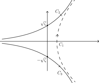
. Let us first consider the case , and
deform the image of the contour under the mapping
defined in (4.6) to the steepest descent path of in
the -plane which passes through . We denote the
path by . Similarly, we deform the image of the contour
, and denote the steepest descent path passing through
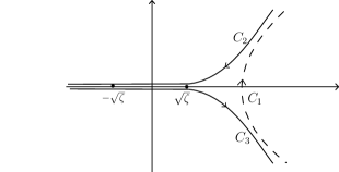
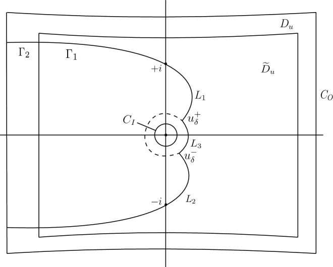
by ; see Figure 1. Next, we consider the case
. Note that here the saddle points are
real, and that the contours and pass through both of
them; see Figure 2. Clearly, in both cases, is the reflection
of with respect to the real axis in the -plane.
Let denote the dotted curve shown in Figures 1 and 2, and recall the identities and . A combination of (4.1), (4.4), (4.5) and (4.6) then gives
| (4.9) |
where
| (4.10) |
4.1 When is bounded
Following the standard integration-by-parts procedure [11, p.368], we define recursively
| (4.11) | |||||
| (4.12) |
Furthermore, expand
| (4.13) |
From (4.9), (4.11), (4.12) and (4.13), it follows
| (4.14) | ||||
where
| (4.15) |
and the coefficients are given by
| (4.16) |
In the present case, or, equivalently, are bounded. Thus is also bounded in view of (4.7). Therefore, it is easy to prove that (4.1) is asymptotic; for details, see [11, p.371-372].
4.2 When
When , by (2.9) the saddle points approach , respectively, along the line . In view of (4.7), this is equivalent to saying that . To prove that (4.1) is also asymptotic in this case, we rewrite the expansion in (4.1) as
| (4.17) | ||||
where is the same as in (4.15) and
| (4.18) |
Thus, it is sufficient to first prove the boundedness of the coefficients and , and then establish the asymptotic nature of the error term in (4.2), namely, to prove that there exist positive constants , , and such that
| (4.19) |
where
| (4.20) |
and
for . Note that in the present case, .
From (4.8), we recall that depends on . The value of is obtained by solving the two equations gotten from (4.6) with and replaced respectively by and ; see [11, p.367]. Thus, and hence both depend on the parameters and in (1.3). As and approach zero, may tend to infinity. When the saddle points are bounded, the mapping defined by the cubic transformation (4.6) is analytic, and its derivative is bounded. However, in the present case, the saddle points go to infinity as . Hence, the coefficients , and the function given recursively in (4.11) and (4.12) may all blow up as , where is defined by (4.10). Since the coefficients and in (4.1) are related to and via (4.16) and (4.13), to prove that the expansion in (4.2) is asymptotic when , we must first give estimates for the coefficient functions and . To this end, we shall adopt a method introduced by Olde Daalhuis and Temme [5]. To begin with, we define
| (4.21) |
Using (4.11) and the Cauchy residue theorem, it can be verified that
| (4.22) |
where is the contour consisting of two circles, centering
at , both with radius , where could be as
large as possible until the circles reach the singularities of
in the -plane.
We note that are removable singularities of . However, blows up at the points , where is any integer; see (4.8). To find their image points in the -plane under the mapping (4.6), we take as an example and denote its image point by . The image point of can be treated in a similar manner. By (4.6), we have
| (4.23) |
From (4.6) and (4.7), we also have
| (4.24) |
Subtracting (4.24) from (4.23) gives
| (4.25) |
Since and , from (4.25) it follows that . Therefore, there exists a constant , independent of , and , such that the interior of the two circles with centres at and radius is free of the singularities of in the -plane. Since is now analytic inside the contour , there exists a constant such that
| (4.26) |
for in the domain enclosed by the contour , where
denotes the maximum of the two functions
. Note that as functions
of , are analytic in
the neighbourhood of steepest descent path in the -plane.
We further introduce rational functions and , , defined recursively by
| (4.27) |
where and are given in (4.21). By induction, we can show that and are expressible as
| (4.28) |
where and are constants independent of and . As in (4.22), by Cauchy’s theorem, we have from equations (4.11) and (4.12)
| (4.29) |
where we have used integration-by-parts to derive the second equality. The second term in the second equality vanishes because is as and all poles of that function lie inside ; see (4.28). Similarly, we also have
| (4.30) |
Using (4.28), it is easy to obtain the estimates
| (4.31) |
for on and inside the contour and . Here and thereafter, is used as a generic symbol for constants independent of , , and . Substituting (4.31) into (4.29) and (4.30) gives
| (4.32) |
and
| (4.33) |
Therefore, and are both bounded for
in the neighbourhood of steepest descent path in the
-plane, and of course for in the neighbourhood of
. Thus we have the boundedness of the coefficients
and .
To estimate , we use the rational functions , , defined recursively by
| (4.34) |
These functions were also introduced by Olde Daalhuis and Temme [5]. They showed by induction that can be written as
| (4.35) |
where do not depend on , and . Similar to (4.29), we have
| (4.36) |
where is the same contour used in (4.29) and lies inside two disks centered at and with radius . It is easy to verify from (4.35) that
| (4.37) |
and from (4.36) that
| (4.38) |
Substituting (4.38) into (4.20) gives (4.19); for details, see [5, p.311-312]. Note that to make the expansion (4.2) asymptotic, we require to be large.
5 BESSEL-TYPE EXPANSION
In the case of Hahn Polynomials given
in (1.1), Sharapodinov [10] has
given an asymptotic formula involving Jacobi polynomials when the
parameters satisfy , and , where is a positive constant. The values of
the variable are also required to be large; more precisely,
and is a small number.
Although discrete Chebyshev polynomials given in
(1.2) is a special case of the Hahn
polynomials, the values of the parameters are ; that
is, Sharapodinov’s result does not include our case. However, since
the leading term in the uniform asymptotic expansion of the Jacobi
polynomials is a Bessel function (see [7, p.451]), the
work of Sharapodinov did inspire us to look for an asymptotic
expansion for involving Bessel functions, when the
parameters and in (1.3) satisfy and the variable is large. Our method differs completely
from that of
Sharapodinov.
Returning to (2.1), and making the change of variable , we have
| (5.1) |
where
| (5.2) |
the curve starts at , runs along the lower
edge of the positive real line towards , encircles the point
in the clockwise direction and returns to along the
upper edge of the positive real line. Note that since , there is no need to have a cut from the origin to
infinity.
The saddle point of in the -plane is given by
| (5.3) |
cf.(2.5), where the -plane is cut along two line segments joining to the two conjugate points , and the branch of the square root is chosen so that as . From (5.3), we have
| (5.4) |
where is a positive constant, and for ,
| (5.5) |
where and mean limits approaching from the right-hand side of the cut and the left-hand side of the cut, respectively. Moreover, easy calculation shows that for any , is not a real number on the cut in the -plane. Following the same argument given prior to (3.2), we introduce the mapping
| (5.6) |
with the correspondence between the saddle points and given by
| (5.7) |
Coupling (5.6) and (5.7) yields
| (5.8) |
The zeros of are given by
| (5.9) |
where is the relavant saddle point given in . By straightforward calculation, we have
| (5.10) |
Note that we have when , and when . For any fixed , we can deform the original interval of integration into a steepest descent path , passing through . Also note that is not on , unless . Moreover, if , then and is the real interval . In our case, there is only one point on the path in the -plane (see (5.1)), where it crosses the real line. Let us denote this point by . When , the mapping which we have introduced in (5.6) becomes singular at the point , since in (5.10) blows up. However for this particular case, we only need to slightly modify the path by replacing part of the original path near this point by a small half circle as shown in Figure 3.
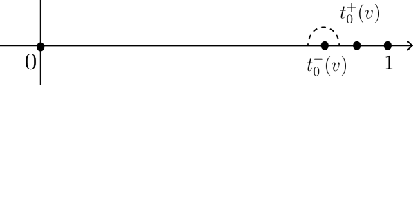
The corresponding integration path in the -plane following the
mapping (5.6) also needs to be modified.
However, this small modification on the integration path will not
affect the following argument and calculation. With this in mind, we
will simply ignore this particular case, and proceed with the
assumption that the integration path in the -plane is always
for all , and that
will not blow up in the neighbourhood of the path.
Thus, from (5.1) and (5.6), we have
| (5.11) |
Here, we rewrite the phase function as
| (5.12) |
Recalling the statements following (5.2) and (5.3), we know that there are only two cuts in the -plane: one along the infinite interval and the other along the bent line joining the conjugate points and passing through the origin. To find the saddle points of , we set
and obtain
| (5.13) |
Since (5.1) is obtained from (2.1) by making the change of variable , (5.13) can also be derived from (2.9).
Note that in this case, . Furthermore, since
, the quantity inside the square root is positive.
Hence, are distinct, and approach .
Define
where is some constant to be determined. The saddle points of are
| (5.14) |
Make the transformation
| (5.15) |
with
| (5.16) |
Note the fact that , where are given in (2.3) and (2.4). This can be seen from (2.6) and the change of variable that we have made. Thus, substituting (5.16) into (5.15) gives
| (5.17) |
and
| (5.18) |
when and . Moreover, from (5.15) we have
| (5.19) |
Here we have made use of the equality
.
Coupling (5.11) and (5.15), the integral representation of becomes
| (5.20) |
where
| (5.21) |
and the contour starts from , encircles the point in the counterclockwise direction and returns to . For , we define recursively
| (5.22) | |||||
| (5.23) |
where given in (5.21). Furthermore, we expand and at , and write
| (5.24) |
It is easy to see that
| (5.25) |
From (5.20), (5.22) and (5.23), we have
| (5.26) | ||||
where
| (5.27) |
and
| (5.28) |
In (5), we have made use of the integral representations of Bessel function and Gamma function
and
see [7, (10.9.19) and (5.9.1)]. Using (5.23) and integration by parts, we can rewrite in (5.28) as
| (5.29) |
Repeating the procedure above, we obtain
| (5.30) |
where
| (5.31) | |||||
| (5.32) | |||||
| (5.33) |
Since involves and
depends on the parameters and
in (1.3), the coefficients and in (5.31) and (5.32) also depend
on and . For an estimate on these coefficients, see (5.57) below.
To facilitate the application of expansion (5.30), we recall that the constants and are explicitly given in (5.17) and (5.18), and note that the leading coefficient can be (asymptotically) calculated by using (5.24) and (5.25). Indeed, we have
and
as and . Furthermore, equation (5.39) gives
| (5.34) |
where .
5.1 The mapping in (5.15)
In the case under discussion, and . Thus, since , we have , and the saddle points in (5.13) are complex.
Theorem 1.
Proof.
As in the cases of Charlier polynomials [9] and Meixner polynomials [3], we introduce an intermediate variable defined by
| (5.35) |
where is the relevant saddle point given in (5.3).
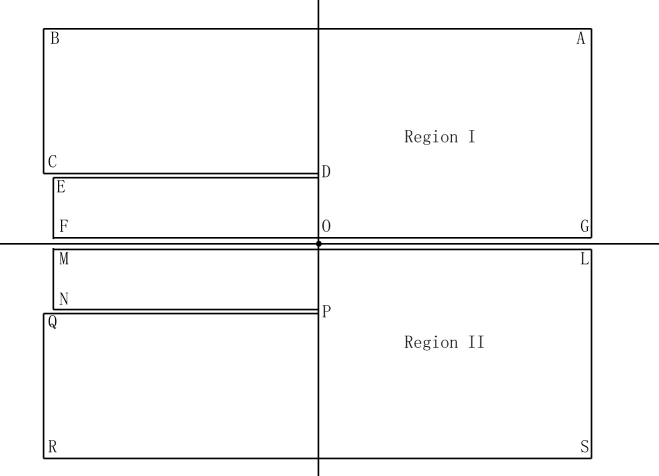
We consider the upper half of the -plane. Since the functions
and are both symmetric with
respect to the real line, the case for the lower half of the
-plane can be handled in the same manner. To avoid
multi-valuedness around the saddle point, we divide the upper half
of the -plane into two parts by using the steepest descent path
through , i.e., the point denoted by ; see Figure
4. Call the two parts region I and region III. Note that
there are two branch cuts: one along the infinite interval
, and the other along the line segment joining to
, which was introduced in (5.3). We denoted the point
by the letter in Figure 4.
As traverses along the boundary of region I, the
image point traverses along the corresponding boundary of a
region in the -plane; see Figure 5. In Figure
7, we draw the boundary of the region, corresponding to
region I, in the -plane. The image point
traverses along the boundary of the same region shown in Figure
5. Note that we have used an arc to avoid the
cut . The boundary curves and in the -plane are
rather arbitrary; for convenience, we choose them to be the ones
whose images
in the -plane are as indicated in Figure 5.
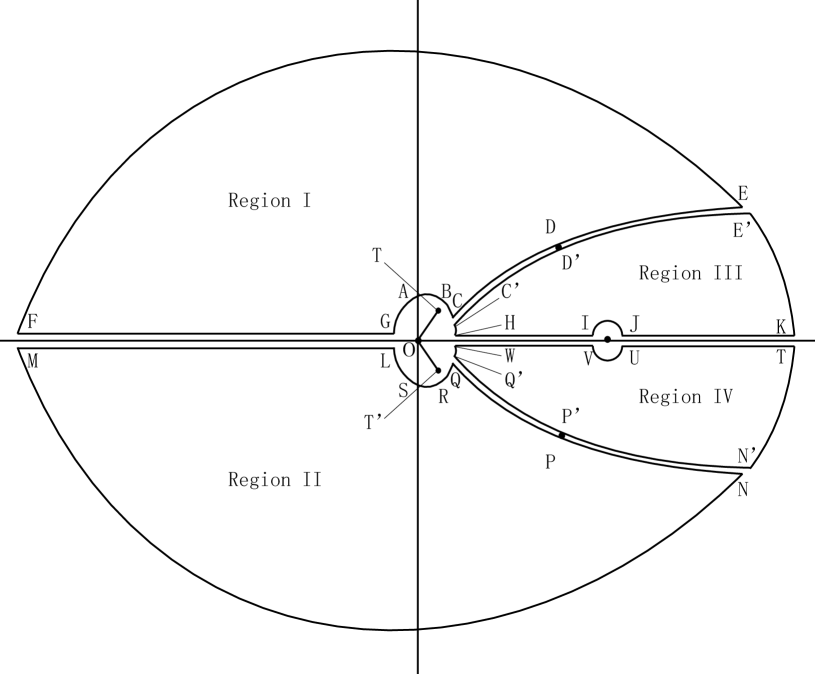
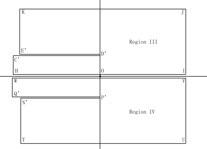
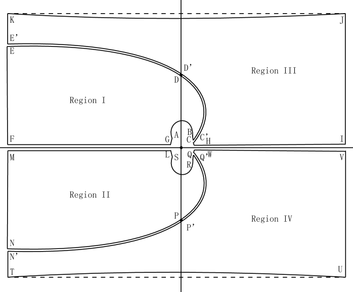
From (5.15), it is readily seen that the mapping is the composite function of and . We have just verified that this mapping is one-to-one on the boundary of region I. By the same argument, one can prove that this mapping is also one-to-one on the boundary of region III. For the image of region III in the intermediate -plane, see Figure 6. In the -plane, we let denote the union of the regions I to IV, with outer boundary , and inner boundary ; see Figure 7. Under the mapping , we express the images of parts of the outer and inner boundaries of in the -plane as follows:
| (5.36) |
where is any fixed constant, and is a generic symbol
for a constant in
. Furthermore, we denote by the corresponding region of in the -plane.
By Theorem 1.2.2 of [13, p.12], the mapping is one-to-one in the interior of both regions I and III in the upper half of the -plane. As explained earlier, the one-to-one property of this mapping in the lower half of the -plane can be established by using the symmetry of the functions with respect to the real axis. Note that the only possible singular points of the mapping in are at . Since the images of these points in the -plane (i.e., ) are bounded, the mapping is in fact one-to-one and analytic in .
∎
5.2 Analyticity of
We now investigate the function given in (5.21). By (5.10) and (5.19), we have
| (5.37) |
when and , and
| (5.38) |
when and , where and is defined in the previous subsection. Note that is excluded from . It is easy to see that is bounded by a constant, independent of and , as for and . Therefore, is analytic in for in the neighbourhood of ). Moreover, is also analytic in for , since the only singularities in are both removable; indeed, we have
| (5.39) |
when and , and by the equation following (5.19) we also have
| (5.40) |
when and . To reach (5.40), we have written as and
move inside the square root in
at ; see
(5.19).
For the analysis to be used in the next subsection, we now give an
estimate for when lies on the boundaries of ,
i.e, the outer boundary and the inner boundary
shown in Figure 7. For convenience, let
us denote the outer boundary by and the inner boundary by
.
First, we show that for on the inner boundary ,
| (5.41) |
where and , , are used, here and thereafter, as generic symbols for constants independent of , , , and . Recall from (5.18) that as . To prove (5.41), we take the part of the inner boundary as an illustration. Using (5.36), we obtain
| (5.42) |
Since , from the equality in (5.42) we have . Therefore,
| (5.43) |
Rewriting (5.42) gives
| (5.44) |
which lead to . Substituting (5.43) into the right-hand side of the last inequality, and combining the resulting inequality with (5.43), we obtain (5.41) immediately. Similarly, for on the outer boundary , we have the estimates
| (5.45) |
5.3 Error bounds for the remainder
To prove the asymptotic nature of the expansion in (5.30), we need to give precise estimates for its coefficients , in (5.31) and (5.32), and the error term given in (5.33), since the derivative in (5.19) may blow up as approach 0, just like the case in Section 4. Because the coefficients and are related to and by (5.24), (5.31) and (5.32), let us first estimate and . To this end, we define recursively
and
for . By induction, it can be shown that
| (5.47) |
for , where and are constants independent of and (but dependent of ); see [12]. Furthermore, by (5.25), (5.22) and (5.23), it can be proved that
| (5.48) |
and
| (5.49) |
see also [12]. Define ; since in this case
both and , and , we
have , if
, and if .
Using (5.47), (5.41) and (5.45), it is easily verified that
| (5.50) |
for on the inner boundary , and
| (5.51) |
for on the outer boundary , where is used again as a generic symbol for constants independent of , and . Also we have the estimates
| (5.52) |
To see this, we take one part of , namely, as an example; see (5.35) and (5.36), where in (5.35) satisfies . Using the second equality in (5.36), and in polar coordinates, , the last equation is equivalent to
| (5.53) |
Thus
| (5.54) |
Since in this case , we have . By (5.41), and
| (5.55) |
from which the first inequality in (5.52)
follows. The second inequality can be established in a similar
manner.
Since and is analytic in , we have for some constant and for in the neighbourhood of the origin. By a combination of (5.48), (5.49), (5.50), (5.51), (5.52) and (5.46), we obtain
| (5.56) |
for near . Furthermore, by (5.24), (5.31), (5.32) and (5.56), we have
| (5.57) |
To estimate the remainder in (5.33), we split the loop contour into two parts; see Figure 8. The bounded part of the contour, denoted by , is contained in a subdomain of , which has a distance from the outer boundary of (i.e., ), and has a distance from the inner boundary of (i.e., ), and being two constants independent of , and . Note that may become large, whereas may approach zero. The unbounded part of the contour, denoted by , is the rest of the loop outside the subdomain . Put
| (5.58) | |||||
| (5.59) |
As in [5] and [12], it can be shown that is exponentially small in comparison with . To estimate , we also follow [5] and [12] by first deriving an integral representation for . Define recursively
| (5.60) |
for . Using induction, one can easily verify that
| (5.61) |
where are some constants depending only on , and . Similar to (4.36), for we have from (5.22), (5.23) and (5.60) the integral representation
| (5.62) |
From (5.61), it is easy to see that
| (5.63) |
Coupling the above inequalities with (5.52) and (5.62), we obtain
| (5.64) |
for and in the neighbourhood of .
If we divide the integration path into three pieces: the steepest descent path through in the upper half of the -plane, the steepest descent path through in the lower half of the -plane, and the circular arc , denoted by , which joins the steepest descent paths and at and , respectively; see Figure 8. Hence,
| (5.66) |
where , , denotes the integral over the subcontour . Applying the steepest descent method [11, p.84], and using (5.64), it can be easily verified that
| (5.67) |
For , since
is exponentially small in comparison with . Therefore,
| (5.68) |
It is well-known that the Bessel function is bounded when is bounded, and that as ,
| (5.69) |
Coupling the estimates (5.65) and (5.68), and together with (5.69) and (5.57), we can find a constant independent of and such that
| (5.70) |
which establishes the asymptotic nature of the expansion in (5.30), given that . In conclusion, in the case and , (5.30) is an asymptotic expansion.
6 REMAINING CASES
We are now left with only two easy cases to consider.
6.1 , large and bounded
6.2
The case is relatively easy, compared with the case . Let us start with the integral representation (2.23). For fixed , the phase function in (2.23) has a saddle point
| (6.1) |
cf.(2.5). Note that the only difference between in (2.2) and in (2.24) is the choice of branch cuts in the -plane due to the term in and the term in . Similar to (3.1), for any fixed , we have as ; in particular, . By the same reasoning given for (3.2), we introduce the mapping defined by
| (6.2) |
with
| (6.3) |
Coupling (6.3) and (6.2) yields . From (6.2), we have
| (6.4) |
where we have used L’Hspital’s rule for and
| (6.5) |
cf.(3.5). Furthermore, it follows from (6.2) and (2.23) that
| (6.6) |
cf.(3.6). Solving the equation , we obtain the saddle points
| (6.7) |
cf.(2.9). The relevant saddle point on the
integral path is the negative saddle point .
The following procedure is the same as that given in [8]. Recall the Hankel integral for the Gamma function
| (6.8) |
where the contour is a loop starting at , encircling the origin in the counterclockwise direction and returning to . With and replaced by , we obtain
| (6.9) |
where . Make the transformation defined by
| (6.10) |
with
| (6.11) |
where is a constant to be determined. We have from (6.10)
| (6.12) |
where we again have used L’Hspital’s rule for .
References
- [1] R. Beals and R. Wong, Special Functions, A Graduate Text, Cambridge University Press, Cambridge, 2010.
- [2] C. Chester, B. Friedman and F. Ursell, An extension of the method of steepest descents, Proc. Cambridge Philos. Soc. 53 (1957), 599-611.
- [3] X.-S. Jin and R. Wong, Uniform asymptotic expansions for Meixner polynomials, Constr. Approx. 14 (1998), 113-150.
- [4] Y. Lin and R. Wong, Global Asymptotics of the Hahn Polynomials, Analysis and Applications, to appear.
- [5] A. B. Olde Daalhuis and N. M. Temme, Uniform Airy-type expansions of integrals, SIAM J. Math. Anal. 25 (1994), 304-321.
- [6] F. W. J. Olver, Asymptotics and Special Functions, Academic Press, New York, 1974. (Reprinted by A. K. Peters, Wellesley, MA, 1997.)
- [7] F. W. J. Olver, D. W. Lozier, C. W. Clark and R. F. Boisvert, NIST Handbook of Mathematical Functions, Cambridge University Press, Cambridge, 2010.
- [8] J. H. Pan and R. Wong, Uniform Asymptotic Expansions for the Discrete Chebyshev Polynomials, Studies in Applied Mathematics 128 (2012), 337-384.
- [9] Bo, Rui and R. Wong, Uniform asymptotic expansion of Charlier polynomials. Methods and Applications of Analysis 1 (1994), 294-313.
- [10] I. I. Sharapudinov, Asymptotic Properties of Orthogonal Hahn Polynomials in a Discrete Variable, Sbornik: Mathematics, Vol. 68, 1 (1991), 111-132.
- [11] R. Wong, Asymptotic Approximations of Integrals, Academic Press, Boston, 1989. (Reprinted by SIAM, Philadelphia, PA, 2001)
- [12] R. Wong and Y. Q. Zhao, Estimates for the error term in a uniform asymptotic expansion of the Jacobi polynomials. Anal. Appl. (Singap.) 1 (2003), no. 2, 213-241.
- [13] R. Wong, Lecture Notes on Applied Analysis, World Scientific, Singapore, 2010.