Asynchronous Distributed Protocol for Service Provisioning in the Edge-Cloud Continuum

Following the intuition, one would reduce the system costs by placing MSs in the network continuum as close as possible to the cloud, since cloud resources are cheaper and this may prevent future migrations. However, such an approach may make the algorithm fail to find feasible solutions, even when they exist [6].

Our solution to this conflict between feasibility and cost-efficiency is inspired to [6]. The proposed DAPP-ECC algorithm initially assigns – or, better, reserves – CPU for each request as close as possible to the edge. We dub this stage Seek a Feasible Solution (SFS). Once such a solution is found, the protocol Pushes Up (PU) the MSs as much as possible towards the cloud, to reduce costs. If SFS cannot find a feasible solution, non-critical MSs will be migrated via the Push-Down (PD) procedure, to make room for a critical MS.

We now detail the algorithmic framework we developed. We will denote by $\tilde{\mathcal{M}}$ a list of currently unassigned requests, and by $\mathcal{P}^{U}$ a list of assigned requests that may be pushed-up to a closer-to-the-cloud datacenter, to reduce costs. Let $\mathcal{P}^{D}$ denote a set of push-down requests. $a_{s}$ denotes the available capacity on datacenter $s$. Upon system initialization, each datacenter $s$ assigns $\tilde{\mathcal{M}}_{s}=\mathcal{P}^{U}_{s}=\mathcal{P}^{D}_{s}=\emptyset$ and $a_{s}=C_{s}$.

F-mode. Intuitively, a run of $s$.PD() indicates that a recent run of SFS() – either in $s$, or in an ancestor of $s$ – failed, and hence called PD(). Since in such a case, there is a high risk of failing again, the algorithm should focus on finding a feasible solution, rather than reducing costs: it does not make sense to push-up MSs just to push them back down slightly later. Hence, we define an F (feasibility)-mode of the protocol. Each time $s$.PD() is called, $s$ enters $F$-mode (if it was not already in $F$-mode), and remains so for some pre-configured F-mode period. While in $F$-mode, DAPP-ECC does not initiate new push-up requests, and only replies to existing push-up requests with the minimum necessary details to prevent deadlocks. If $s$.SFS() does not find a feasible solution while $s$ is in $F$-mode, DAPP-ECC terminates with a failure.

Accumulation delay. Theoretically, each attempt to place a single MS may result in a unique run of PD  that involves all the datacenters, thus incurring excessive overhead. To avoid such case, observe that, typically, several users move together in the same direction (e.g., cars moving simultaneously on the road, on the same trajectory). Naively, such a scenario may translate to multiple invocations of DAPP-ECC, each of them for placing a single request. To tackle this problem, we introduce short accumulation delays to our protocol. We let each datacenter receiving a SFS message wait for a short SFS accumulation delay before it begins handling the new request. To deter long service delays or even deadlocks, each datacenter maintains a single SFS accumulation delay timer that operates as follows: if a run of SFS reaches Ln. 3 in Alg. 1 while no SFS accumulation delay timer is ticking, the procedure initiates a new SFS accumulation delay timer. This current run of SFS, as well as all the subsequent runs, halt. After the SFS accumulation delay terminates, only a single SFS process resumes (see Alg. 1, Ln. 3).

Likewise, to initiate fewer runs of PD(), we let each datacenter retain a single PD accumulation delay mechanism that works similarly to the SFS accumulation delay timer. Significantly, the accumulation delay only impacts the time until the protocol finds a new feasible placement, not the delay experienced by applications in the data plane. We assess the impact of the accumulation delay in Sec. V-B.

Service area, network, and datacenters. We consider two mobility traces, representing real-world scenarios with distinct characteristics: the vehicular traffic within the centers of the cities of (i) Luxembourg [16], and (ii) the Principality of Monaco [17]. For the PoAs, we rely on real-world antenna locations, publicly available in [18]. For each simulated area, we consider the antennas of the cellular telecom provider having the largest number of antennas in the simulated area. For both traces, we consider the 8:20-8:30 am rush hour period. Further details about the mobility traces can be found in [6, 16, 17].

Network and datacenters. The cloud-edge continuum is structure as a 6-height tree; a topology level is denoted by $\ell\in\{0,1,\dots,5\}$. The leaves (level 0) are the datacenters co-located with the PoAs (antennas). Similarly to [9, 8, 12], the higher levels $5,4,3,2,1$ recursively partition the simulated area. In both Luxembourg and Monaco, if no PoAs exist in a particular rectangle, the respective datacenters are pruned from the tree. The CPU capacity increases with the level $\ell$ to reflect the larger computational capacity in datacenters closer to the cloud. Denoting the CPU capacity at each leaf datacenter by $C_{\text{cpu}}$, the CPU capacity in level $\ell$ is $(\ell+1)\cdot C_{\text{cpu}}$.

Services and costs. Each vehicle that enters the considered geographical area is randomly marked as requesting either real time (RT) or non-RT services, with some probability defined later. We calculate $\mathcal{S}_{r}$, $\beta^{r,s}$, and $\psi^{c}(r,s)$ for each $r\in\mathcal{R},s\in\mathcal{S}$ using the GFA algorithm and the same data-plane latency parameters as in [6]. We thus obtain the following values. Each RT request can be placed on levels 0, 1, or 2 in the tree, requiring CPU of 17, 17, and 19 GHz, associated with costs of 544, 278, and 164, respectively. Each non-RT request can be placed on any level, with a fixed allocated CPU of 17 GHz and associated costs of 544, 278, 148, 86, 58, and 47 for placing the MS on levels 0, 1, 2, 3, 4 and 5, respectively. The migration cost is $\psi^{m}(r,s,s^{\prime})=600$ for every request $r$ and datacenters $s,s^{\prime}$.

Delays. The delay experienced by each packet consists of (i) transmission delay and (ii) propagation delay.

The transmission delay is calculated as the packet’s size over the capacity allocated for the control plane at each link, through a dedicated network slice. We assume that this capacity is 10 Mbps. We now detail the size of each field in the messages exchanged by DAPP-ECC. As DAPP-ECC uses only single-hop packets, we assume a fixed 80-bits header. The IDs of datacenters, and requests, are represented using 12-bits, and 14-bits. Each MS belongs to a concrete class of timing constraint, expressed through a 4-bit classId. The CPU allocation of an MS on a datacenter $\beta^{r,s}$ is represented through a 5-bits field. deficitCpu is at most the highest capacity of any single datacenter; we assume that this requires 16 bits. For the propagation delay, we use a pessimistic approach, where the length of every single link in the network corresponds to the diameter of the simulated area, and the propagation speed is $2\cdot 10^{8}~{}\text{ms}^{-1}$. Consequently, the propagation delay of each link in Luxembourg and Monaco is $22~{}\mu\text{s}$ and $8~{}\mu\text{s}$ (resp.). For a datacenter at level $\ell$, SFS accumulation delay, and PD accumulation delay are $(\ell+1)\cdot T^{SFS}_{ad}$, and $(\ell+1)\cdot T^{PD}_{ad}$ (resp.). We assign $T^{SFS}_{ad}=0.1$ ms and $T^{PD}_{ad}=0.4$ ms. $F$-mode period (recall Sec. IV-C) is 10 s.

Benchmark algorithms. We are unaware of any fully distributed, asynchronous algorithm for the PMP. Hence, we consider centralized placement schemes that identify the currently critical and new users once in a second and solve the respective PMP. We will consider the following algorithms.

Lower Bound (LBound): An optimal solution to the PMP that can place fractions of an MS on distinct datacenters. Also, the LP formulation considers all MSs in the system every 1 s period, not just critical MSs. Hence, it serves as a lower bound on the cost of any feasible solution to the problem.

F-Fit: It places each request $r$ on the lowest datacenter in $\mathcal{S}_{r}$ that has sufficient available resources to place MS $\mathbf{m}^{r}$. This is an adaptation to our problem of the placement algorithm proposed in Sec. IV.B in [19].

BUPU [6]: It consists of two stages. At the bottom-up, it places all the critical and new MSs as low as possible. If this stage fails to place an MS while considering datacenter $s$, the algorithm re-places all the MSs associated with $s$’s sub-tree from scratch. Later, BUPU performs a push-up stage similar to our DAPP-ECC’s PU() procedure.

Simulation methodology. We simulate users’ mobility using SUMO [20]. The benchmark algorithms use the Python code publicly available in [21]. DAPP-ECC is implemented using OMNeT++ network simulator [22]. Each new user, or an existing user which becomes critical, invokes a run of DAPP-ECC datacenter co-located with the user’s PoA. DAPP-ECC’s code is available in [23]. LBound is computed using Gurobi optimizer [24].

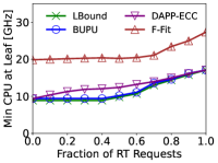
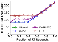
We now study the amount of resources each algorithm requires to find a feasible solution. We vary the fraction of RT MSs with respect to the total MSs. For each setting, a binary search is used to find the minimum amount of resources needed by the algorithm in question to successfully place all the critical MSs along the trace. Fig. 1 presents the results of this experiment. The amount of CPU required by BUPU is almost identical to the optimal value. Despite being fully distributed and asynchronous, the amount of CPU needed by DAPP-ECC is only slightly higher than BUPU. Finally, F-Fit requires a processing capacity that is 50% to 100% higher than LBound to provide a feasible solution.

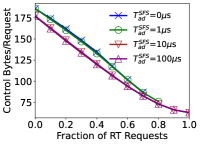
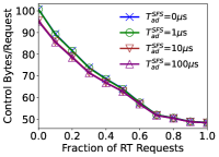
For each simulated scenario, we now set the CPU resources to 10% above the amount of resources required by LBound to find a feasible solution when 100% of the requests are RT. While maintaining this amount of CPU resources, we vary the ratio of RT requests, and measure the overall amount of data for signaling used by DAPP-ECC. Fig. 2 presents the per-request signaling overhead, defined as the overall signaling data exchanged by DAPP-ECC (“control bytes”) over the overall number of critical/new requests along the trace. We consider several values of the SFS accumulation delay parameter $T^{SFS}_{ad}$. A run of PD() may migrate also non-critical MSs, thus incurring a higher overhead than PU(). Hence, we set $T^{PD}_{ad}=4\cdot T^{SFS}_{ad}$. The results show that increasing the fraction of RT requests decreases the signaling overhead. The reason is that RT requests can be placed only in the three lowest levels in the tree, thus avoiding any signaling message between higher-level datacenters. When increasing the accumulation delays, the protocol aggregates more requests before sending a message, thus decreasing the signaling overhead. However, an accumulation delay of about $10~{}\mu\text{s}$ suffices. We stress that the accumulation delay only impacts the time until the protocol finds a new feasible placement, not the delay experienced by the user’s application. Indeed, delaying the migration decision may deteriorate the user’s QoE. However, this performance deterioration can be mitigated using an efficient prediction mechanism for the user’s mobility. Furthermore, in practical scenarios, an accumulation delay of about $10~{}\mu\text{s}$ may be negligible compared to the more considerable delay incurred by the migration process. Finally, in all the settings considered, the signaling overhead associated with each request is about $100$ bytes. Thus, we can claim a very low overhead for DAPP-ECC.

In our next experiment, we compare the cost of various solutions for the PMP. We set the ratio of RT requests to 30%, and vary the resource augmentation.

The results (not detailed here due to lack of space) show that the costs obtained by BUPU and DAPP-ECC are almost identical, and both are up to 10% higher than LBound (depending on the concrete setting). That is, despite being distributed and asynchronous, DAPP-ECC obtain costs that are almost identical to those obtained by BUPU, which relies on a centralized controller with an always-accurate view of the system state. F-Fit typically only finds any feasible solution when resources are abundant, in which case all the placement algorithms easily obtain close-to-optimal costs.

References

- [1] B. Kar et al., “QoS violation probability minimization in federating vehicular-fogs with cloud and edge systems,” IEEE Transactions on Vehicular Technology, vol. 70, no. 12, pp. 13 270–13 280, 2021.
- [2] D. Zhao et al., “Mobile-aware service function chain migration in cloud–fog computing,” Future Generation Computer Systems, vol. 96, pp. 591–604, 2019.
- [3] S. Svorobej et al., “Orchestration from the cloud to the edge,” The Cloud-to-Thing Continuum, pp. 61–77, 2020.
- [4] Y.-D. Lin, C.-C. Wang, C.-Y. Huang, and Y.-C. Lai, “Hierarchical cord for NFV datacenters: resource allocation with cost-latency tradeoff,” IEEE Network, vol. 32, no. 5, pp. 124–130, 2018.
- [5] L. Tong, Y. Li, and W. Gao, “A hierarchical edge cloud architecture for mobile computing,” in IEEE INFOCOM, 2016, pp. 1–9.
- [6] I. Cohen et al., “Dynamic service provisioning in the edge-cloud continuum with bounded resources,” IEEE Transaction on Networking, in press, 2023.
- [7] H. Yu, J. Yang, and C. Fung, “Elastic network service chain with fine-grained vertical scaling,” in IEEE GLOBECOM, 2018, pp. 1–7.
- [8] I. Leyva-Pupo et al., “Dynamic scheduling and optimal reconfiguration of UPF placement in 5G networks,” in ACM MSWiM, 2020, pp. 103–111.
- [9] X. Sun and N. Ansari, “PRIMAL: Profit maximization avatar placement for mobile edge computing,” in IEEE ICC, 2016, pp. 1–6.
- [10] I. Cohen et al., “Parallel VM deployment with provable guarantees,” in IFIP Networking, 2021, pp. 1–9.
- [11] A. De La Oliva et al., “Final 5g-crosshaul system design and economic analysis,” 5G-Crosshaul public deliverable, 2017.
- [12] T. Ouyang et al., “Adaptive user-managed service placement for mobile edge computing: An online learning approach,” in IEEE INFOCOM, 2019, pp. 1468–1476.
- [13] S. Wang et al., “Dynamic service migration in mobile edge-clouds,” in IEEE IFIP Networking, 2015, pp. 1–9.
- [14] Martín-Pérez et al., “OKpi: All-KPI network slicing through efficient resource allocation,” in IEEE INFOCOM, 2020, pp. 804–813.
- [15] M. Nguyen, M. Dolati, and M. Ghaderi, “Deadline-aware SFC orchestration under demand uncertainty,” IEEE Transactions on Network and Service Management, pp. 2275–2290, 2020.
- [16] L. Codecá et al., “Luxembourg SUMO traffic (LuST) scenario: Traffic demand evaluation,” IEEE Intelligent Transportation Systems Magazine, pp. 52–63, 2017.
- [17] L. Codeca and J. Härri, “Monaco SUMO traffic (MoST) scenario: A 3D mobility scenario for cooperative ITS,” EPiC Series in Engineering, vol. 2, pp. 43–55, 2018.
- [18] “Opencellid,” https://opencellid.org/, accessed on 3.10.2021.
- [19] M. Goudarzi, M. Palaniswami, and R. Buyya, “A distributed application placement and migration management techniques for edge and fog computing environments,” in IEEE FedCSIS, 2021, pp. 37–56.
- [20] P. Alvarez et al., “Microscopic traffic simulation using sumo,” in IEEE International Conference on Intelligent Transportation Systems, 2018.
- [21] “Service function chains migration.” [Online]. Available: https://github.com/ofanan/SFC_migration
- [22] “OMNeT++ discrete event simulator,” 2023. [Online]. Available: https://omnetpp.org
- [23] “Distributed SFC migration.” [Online]. Available: https://github.com/ofanan/Distributed_SFC_migration
- [24] “Gurobi optimizer reference manual,” 2023. [Online]. Available: https://www.gurobi.com
- [25] C. Puliafito et al., “Companion fog computing: Supporting things mobility through container migration at the edge,” in IEEE SMARTCOMP, 2018, pp. 97–105.
- [26] M. S. Hung and J. C. Fisk, “An algorithm for 0-1 multiple-knapsack problems,” Naval Research Logistics Quarterly, vol. 25, no. 3, pp. 571–579, 1978.
- [27] K. Ha et al., “You can teach elephants to dance: Agile VM handoff for edge computing,” in ACM/IEEE SEC, 2017, pp. 1–14.
- [28] T. Subramanya and R. Riggio, “Centralized and federated learning for predictive VNF autoscaling in multi-domain 5G networks and beyond,” IEEE TNSM, vol. 18, no. 1, pp. 63–78, 2021.