Date of publication xxxx 00, 0000, date of current version xxxx 00, 0000. 10.1109/ACCESS.2022.0122113
This work was supported in part by the Japan Science and Technology Agency (JST) PRESTO under Grant JPMJPR1935, and in part by Japan Society for the Promotion of Science (JSPS) KAKENHI under Grant 20H02145. This work was also supported in part by the Japan Science and Technology Agency (JST) FLOuRISH.
Corresponding author: Yang Li (e-mail: lytuat@msp-lab.org).
Attention-based Graph Convolution Fusing Latent Structures and Multiple Features for Graph Neural Networks
Abstract
We present an attention-based spatial graph convolution (AGC) for graph neural networks (GNNs). Existing AGCs focus on only using node-wise features and utilizing one type of attention function when calculating attention weights. Instead, we propose two methods to improve the representational power of AGCs by utilizing 1) structural information in a high-dimensional space and 2) multiple attention functions when calculating their weights. The first method computes a local structure representation of a graph in a high-dimensional space. The second method utilizes multiple attention functions simultaneously in one AGC. Both approaches can be combined. We also propose a GNN for the classification of point clouds and that for the prediction of point labels in a point cloud based on the proposed AGC. According to experiments, the proposed GNNs perform better than existing methods. Our codes open at https://github.com/liyang-tuat/SFAGC.
Index Terms:
Attention-based graph convolution, graph neural network, 3D point cloud, deep learning.=-21pt
I Introduction
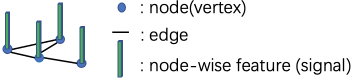
We often encounter irregularly structured data (signals) in the real world where they do not have a fixed spatial sampling frequency. Such data include opinions on social networks, the number of passengers on traffic networks, coordinates of 3D point clouds, and so on.
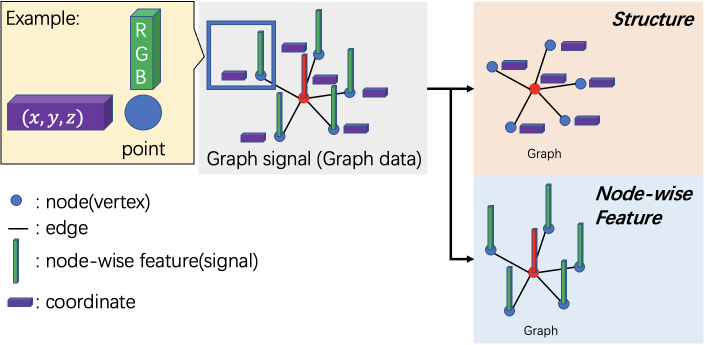
Deep neural networks have been widely used in recent years to detect, segment, and recognize regular structured data [1, 2, 3]. However, classical deep learning methods can not directly process the irregularly structured data mentioned above. They can be mathematically represented as data associated with a graph. An example of graph-structured data, that is, graph signals, is shown in Fig. 1. Deep neural networks for graph signals are called graph neural networks (GNNs): They have received a lot of attention [4, 5, 6, 7].
GNNs typically contain multiple graph convolution (GC) layers. The primary mechanism of GCs is to iteratively aggregate (i.e., filter) features from neighbors before integrating the aggregated information with that of the target node [4, 5, 8, 9]. In many existing GC methods, the node-wise features are typically utilized [10, 11, 12, 13]. Furthermore, it is observed that GCs are a special form of Laplacian smoothing [14]. This low-pass filtering effect often results in over-smoothing [4, 5, 14]. Over-smoothing means that the node-wise feature values become indistinguishable across nodes. Intuitively, representational power of GCs refers to the ability to distinguish different nodes [15]. Therefore, over-smoothing may negatively affect the performance of GNNs.
To improve the representational power of GCs, attention-based spatial graph convolutions (AGCs) such as graph attention networks (GATs) [16] have been proposed. AGCs are believed to have high representational power than the direct spatial methods because they can use features on neighboring nodes through the attention weights. However, there exist two major limitations in existing AGCs: 1) They may lose the structural information of the surrounding neighboring nodes, especially in a high-dimensional space. 2) When calculating attention weights for each neighboring node, only one type of attention function is used, e.g., dot-production, subtraction, or concatenation. Different types of attention functions will lead to different attention weights, which affect the representational power of AGCs.
In this paper, we propose a new AGC to overcome the above-mentioned limitations. First, we propose a local structure projection aggregation. This operation aggregates the structural information of neighboring nodes of a target node. Second, we also propose an AGC that utilizes multiple-type attention functions. We can simultaneously utilize these two methods to present the attention-based graph convolution fusing latent structures and multiple features (SFAGC). Our contributions are summarized as follows:
-
1.
By using local structure projection aggregation, we can obtain a representation of the local structural information of the graph in high-dimensional space in an AGC. This allows the convolved nodes to contain richer information than existing methods.
-
2.
By using multiple-type attention functions simultaneously, we can obtain better attention weights than the single attention function.
-
3.
We construct GNNs for graph and node classifications based on the proposed AGC with 3D point clouds. We demonstrate that GNNs using our method present higher classification accuracies than existing methods through experiments on ModelNet [17] for graph classification and ShapeNet [18] for node classification.
Notation: An undirected and unweighted graph is defined as , where is a set of nodes, and is a set of edges. The adjacency matrix of is denoted as . is the diagonal degree matrix. The graph Laplacian is defined as . is the matrix whose elements in the diagonal are 1.
Here, represents a feature vector on the node , and is the number of features in . represents a coordinate of the node , and is the dimension of coordinate in .
The non-linearity function is denoted as . The set of neighboring nodes is in which its cardinality is denoted as . A multilayer perceptron (MLP) layer is represented as . A channel-wise avg-pooling is denoted as . A channel-wise max-pooling is denoted as . The vector concatenation operation is denoted as . The SoftMax operation is represented as .
II Preliminary
In this section, we present related work for the proposed GC.
II-A Graph Convolutions
The mechanism of GCs is based on message passing. Message passing involves iteratively aggregating information from neighboring nodes and then integrating the aggregated information with that of the target node [4, 5].
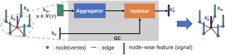
Typically, a GC has two parts, i.e., an aggregator and an updater. The aggregator is to collect and aggregate the node-wise features of neighboring nodes. The updater merges the aggregated features into the target node to update the node-wise features of the target node. These two parts are illustrated in Fig. 2.
Existing GCs can be classified into spectral and spatial methods. Furthermore, spatial methods can be classified into direct and attention-based methods. We briefly introduce them in the following.
II-A1 Spectral methods
In the spectral methods, the aggregation operation is carried out in the graph Fourier domain. Eigenvectors of graph Laplacian are known as the graph Fourier bases [1, 19, 8]. In order to reduce the computational complexity for large graphs, polynomial approximations of graph filters are often utilized [10, 20, 11].
GCN [12] further reduces computational complexity through the first-order graph filters. It can be formulated as follows:
| (1) |
where is the set of node-wise features, is the adjacency matrix with self-loops, and is a learnable weight matrix.
II-A2 Spatial methods
Spatial methods are a counterpart of spectral methods. As we described above, spatial methods can be classified into direct and attention-based methods. Direct spatial methods directly use the node-wise features and the aggregation operation is carried out spatially. A representative method for direct spatial methods is GraphSAGE [13], which treats each neighbor equally with mean aggregation.
Later, attention-based spatial methods are proposed. Instead of treating all neighboring nodes equally, attention-based methods calculate an attention weight for each neighboring node. Then, they use the weighted sum to aggregate features of neighboring nodes. GAT [16] is a representative method for attention-based spatial methods. It is composed of three steps. In the first step, the learnable weights are multiplied by the node-wise features, i.e., , where is the learnable weights. The second step computes attention weights as follows:
| (2) |
where is learnable weights. In the third step, the node-wise features of a target node is updated as follows:
| (3) |
However, as mentioned earlier, existing methods ignore the structural information of neighboring nodes in the high-dimensional space, and use only one type of attention function when calculating an attention weight for each neighboring node.
In contrast to the existing methods, we first focus on computing a representation of the structure of neighboring nodes in high-dimensional feature space and installing them into a spatial GC. Second, we use multiple types of attention functions simultaneously in an AGC. We use both of these two methods simultaneously to achieve SFAGC.
(a)
(b)
(c)
II-B Strctural features
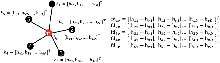
In previous works [21, 22], three structural features, i.e., feature angle, feature distance, and relational embedding, are proposed to describe the structural information between the target node and neighboring nodes. Below, we briefly introduce them since they are also used in our attention-based GCs.
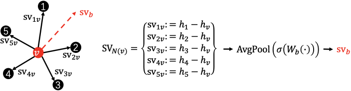
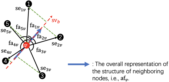
II-B1 Feature angle
Feature angle describes the local structure of neighboring nodes. First, a set of structure vectors pointing from target node to the neighboring nodes are calculated as . Then, a base structure vector is learned from as follows:
| (4) |
where W_b is learnable weights. An example of a base structure vector is shown in Fig. 3
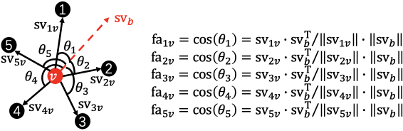
Finally, the cosine of the angle between and is calculated to obtain the feature angle as follows:
| (5) |
An example is shown in Fig. 4 (a).
II-B2 Feature distance
The second structural feature is feature distance. It is the absolute difference between the node-wise features of and represented as follows:
| (6) |
An example is shown in Fig. 4 (b).
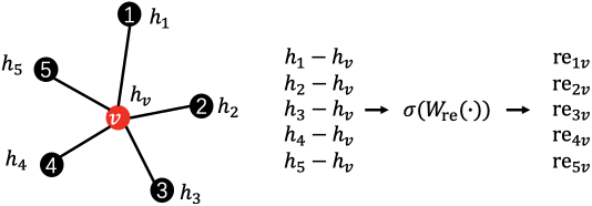
II-B3 Relational embedding
The third structural feature is relational embedding. It can be learned from as follows:
| (7) |
where is learnable weights. An example of it is shown in Fig. 4 (c).
Input:
graph ; input features ;
coordinates ;
weight matrices , , , , , , , , , , , , and ; non-linearity function ; neighborhood function ; MLP layer ; channel-wise avg-pooling ; concatenation operation ; transposition ; SoftMax operation
Output:
Convolved features and updated coordinates for all
III SFAGC
In this section, we introduce SFAGC. As mentioned above, we have two goals: Utilizing 1) the structural information of neighboring nodes in a high-dimensional feature space during a single step GC and 2) multiple-type attention functions simultaneously when calculating the attention weights.
Fig. 5 illustrates an example of a graph with feature vectors in the spatial domain. Spatially distributed nodes often have their coordinates and associated node-wise features, i.e., , where is the coordinate of the node . For example, a 3D color point cloud equips a 3-D coordinate and its node-wise features as RGB values. In the previous structure-aware GCs [21, 22], the node-wise features are simply used as their coordinates. In contrast, the proposed GC, SFAGC, simultaneously considers the coordinates and node-wise features.
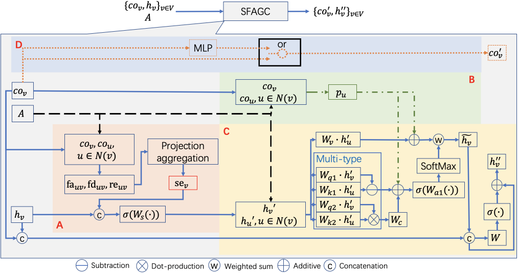
To achieve our goals, the SFAGC has four parts:
- A.
-
Local structure projection aggregation and fusing
- B.
-
Position embedding
- C.
-
Weighted sum aggregation and update
- D.
-
Coordinates processing
SFAGC is illustrated in Fig. 6 and the algorithm of SFAGC is summarized in Algorithm 1. We sequentially introduce these parts.
III-A Local structure projection aggregation and fusing
We propose a projection aggregation operation to obtain the structure representation in the feature space. We then fuse this with the node-wise features of the target node.
III-A1 Local structure projection aggregation
The inputs of this step are the feature angle, feature distance and relational embedding, i.e., , and , introduced in Section II-B. We first compute structure vectors as follows:
| (8) |
where is a learnable weight matrix.
Then, we project each as follows:
| (9) |
Finally, we calculate the summation of the projected structure vectors as follows:
| (10) |
Fig. 7 illustrates an example of the local structure projection aggregation.
III-A2 Fusing structure information with node-wise features
In this step, we fuse the with the as follows:
| (11) |
where is learnable weights.
III-B Position embedding
Position encoding is crucial for a self-attention mechanism because it enables the aggregation operation to adapt to local data structure [23, 24]. Our method directly learns a position embedding, while existing methods use cosine function-based position encoding [24].
We embed the difference of the coordinates between the neighboring node and target node in the feature space. Our position embedding for the node is represented as follows:
| (12) |
where and are learnable weights.
III-C Weighted sum aggregation and update
In this part, we update the node-wise features of the target node .
First, we introduce the calculation steps of the attention weights. Then, we present the weighted sum aggregation and node-wise features update step used in SFAGC.
III-C1 Attention weights
As we described above, we simultaneously use multiple-type attention functions to calculate attention weights. In existing methods [23, 24, 25], the subtraction or dot-production attention function is often utilized to calculate attention weights. Instead of the single attention function, we use these attention functions simultaneously. The subtraction attention function is defined as
| (13) |
where and are learnable weights. The dot-production attention function is represented as
| (14) |
where and are learnable weights.
Then, the two types of attention functions are added with the position embedding p_u as follows:
| (15) |
where is learnable weights that also converts into the same dimensions as .
Finally, is input into a small network to calculate the attention weights between the target node and the neighboring node as follows:
| (16) |
where and are learnable weights, and are the dimensions of the .
III-C2 Weighted-sum aggregation
For and , weighted sum aggregation is calculated as follows:
| (17) |
where is a learnable matrix.
III-C3 Node-wise features update
, and are integrated as follows:
| (18) |
where is learnable weights.
III-D Coordinate update
Finally, we update the coordinate of the target node as follows:
| (19) |
Hereafter, we represent the set of these operations as .
(a)
(b)
| Epoch | 200 | ||||
| Batch size | 16 | ||||
| Learning rate | 0.001 | ||||
| Drop out | 0.3 | ||||
| Phase | Graph convolution layer | Coordinates update | k | [,,,] | |
| Phase1 | SFAGC() | 20 | [3,3,32,64] | ||
| SFAGC | 20 | [32,64,-,64] | |||
| Phase2 | SFAGC | 20 | [32,64,64,64] | ||
| SFAGC | 20 | [64,64,-,128] | |||
| Phase3 | SFAGC | 20 | [64,128,128,256] | ||
| SFAGC | 20 | [128,256,-,256] | |||
| Phase4 | SFAGC | 20 | [64,128,64,128] | ||
| SFAGC | 20 | [64,128,-,128] | |||
| Phase5 | SFAGC | 20 | [128,128,128,256] | ||
| SFAGC | 20 | [128,256,-,256] | |||
| Graph pooling layername | Graph convolution layer | Coordinates update | k | t | [,,,] |
| 1 | SFAGC() | 36 | 512 | [131,131,32,64] | |
| 2 | SFAGC() | 64 | 128 | [320,320,64,128] | |
| 3 | SFAGC() | 64 | 128 | [384,384,128,128] | |
| Pointnet++ layer name | S | r | D | [input channels, output channels] | |
| Pointnet++ | 512 | 0.2 | 32 | [3,64] | |
| 0.4 | 128 | [3,64] | |||
IV Implementation
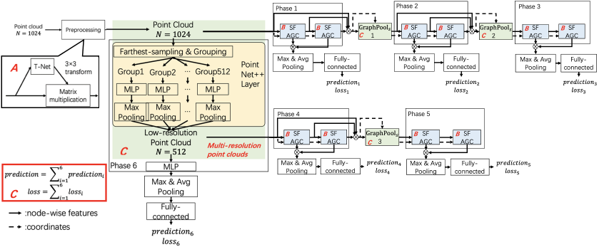
In this section, we construct classification and segmentation networks for 3D point clouds based on SFAGC. Their architectures are illustrated in Fig. 8. In the following, first, we introduce the components shared by the two GNNs. Then, specific implementations for each of the GNNs are introduced.
Here, we suppose that the input point cloud is given by where is the number of points.
IV-A Preprocessing
To alleviate effects on rotations of point clouds, we use the same transformation module as PointNet [26] for preprocessing.
IV-B SFAGC module
The inputs to this module are a set of features obtained from the previous layer and a set of node coordinates in the feature space. Suppose that the set of features output from the previous layer is where is the number of features of the input. For the first module, where is the set of node coordinates.
First, we construct with the -NN graph from where the th node in corresponds to the th feature and the th coordinate .
Recent studies [27, 28] have shown that dynamic graph convolution, i.e., allowing the graph structure to change at each layer, can perform better than that with a fixed graph structure. Therefore, we update coordinates of nodes at each SFAGC module, and we construct different graphs for different SFAGC modules.
IV-C Design of 3D point cloud classification network
Fig. 8 (a) illustrates the architecture of 3D point cloud classification network based on SFAGC. In the following, we describe the details of the building blocks that are specifically designed for point cloud classification.
IV-C1 Multi-resolution point clouds
We use a layer of PointNet++ [29] to generate a low-resolution point cloud. Both global and local information of the point cloud can be obtained through the multi-resolution structure.
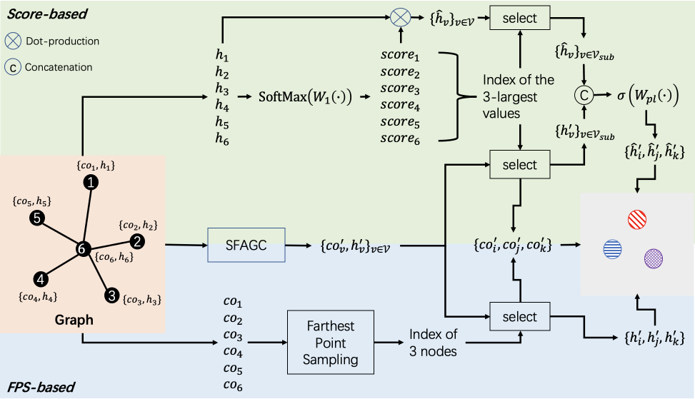
IV-C2 Score-based graph pooling
Effective graph pooling methods are a hot topic in GNNs and graph signal processing [30, 31]. Early work has been done by global pooling of all node-wise features or by using graph coarsening algorithms.
Recently, trainable graph pooling operations DiffPool [32], GraphU-net [33], and AttPool [34] have been proposed. Inspired by the ResNeXt [35], we extend the score-based graph pooling module proposed in SAMGC [22] by introducing the multi-branch architecture. The score-based graph pooling module has three branches: score-based sampling, integration, and SFAGC branches. The architecture of the score-based graph pooling is shown in Fig. 9. In the following, we introduce their details.
In the score-based sampling branch, we propose a scroe-based sampling to find the indices of the best nodes according to their scores. The score associated with each node is first computed as follows:
| (20) |
where is learnable weights. We then sort the nodes in descending order according to their scores. We find the indices of the top nodes as follows:
| (21) |
where is the ranking operation, and it finds the indices of the highest scores.
In the integration branch, node-wise features are multiplied by the node scores as follows:
| (22) |
In the SFAGC branch, the input graph is processed using SFAGC as follows:
| (23) |
Finally, the subset of and the subset of are found using as follows:
| (24) | ||||
and are merged using learnable weights as follows:
| (25) |
where is learnable weights. The score-based graph pooling can be summarized as follows:
| (26) |
IV-C3 Hierarchical prediction architecture
Here, we also use the intermediate supervision technique [36] and the hierarchical prediction architecture (Fig. 8 (a)), as in SAMGC [22]. The advantage of this architecture is that, by combining the outcomes of the different phases, more reliable and robust predictions can be produced [22]. The details are presented below.
We use two SFAGC modules in phase 1 to phase 5. One PointNet++ [29] layer is used in phase 6. Each phase connects with a max pooling layer and an average pooling layer. The outputs are then concatenated and input into a fully connected layer. We calculate the prediction and the classification loss for each phase. The total classification loss is obtained by adding the losses of several phases. Meanwhile, the total prediction is also increased by the predictions of several phases. The following is a representation of this processing:
| (27) | ||||
| (28) |
where is the prediction of the th phase, is the cross-entropy loss of the th phase. and are the total prediction and classification loss, respectively. is the number of phases.
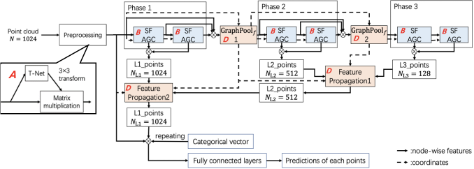
IV-D Design of 3D point cloud segmentation network
Fig. 8 (b) illustrates the architecture of the 3D point cloud segmentation network based on SFAGC. In the following, we describe the details of the building blocks that are specifically designed for point cloud segmentation.
IV-D1 Farthest point sampling-based graph pooling
For point cloud segmentation, we use the graph pooling module to reduce the overall computation cost. Here, we propose the farthest point sampling-based graph pooling (FPS-based graph pooling) by modifying the score-based graph pooling. The architecture of the FPS-based graph pooling is illustrated in Fig. 9. In the following, we introduce its details.
The FPS-based graph pooling has a multi-branch architecture like the score-based graph pooling in Section IV-C2. In contrast to the score-based method, the FPS-based graph pooling has two branches, i.e., the FPS and SFAGC branches.
In the FPS branch, we perform FPS on nodes to obtain indices of the best nodes according to their coordinates. FPS algorithm is widely utilized in 3D point cloud processing [29, 37]. The mechanism of FPS is to iteratively select the node that is farthest from the existing sampled nodes. Therefore, the sampled nodes with the FPS-based sampling are expected to be more evenly distributed than those with the score-based sampling. This branch can be summarized as follows:
| (29) |
where is the indices of the selected nodes, is the farthest point sampling algorithm.
The SFAGC branch is the same as the one that is used in the score-based graph pooling represented as
| (30) |
Finally, the subset of are extracted using as follows:
| (31) |
The FPS-based graph pooling is represented as follows:
| (32) |
IV-D2 Upsampling operation
Graph pooling can be regarded as a downsampling operation. For point cloud segmentation, the network also needs to perform upsampling in order to maitain the number of points. Therefore, the feature propagation used in PointNet++ [29] is also used in our network as the upsampling operation.
| Type | Method | ModelNet40 | ModelNet10 | |||
|---|---|---|---|---|---|---|
| OA | mAcc | OA | mAcc | |||
| Pointwise MLP | PointNet [26] | 89.2% | 86.2% | - | - | |
| Methods | PointNet++ [29] | 90.7% | - | - | - | |
| SRN-PointNet++ [38] | 91.5% | - | - | - | ||
| Transformer-based | PointASNL [37] | 93.2% | - | 95.9% | - | |
| Methods | PCT [39] | 93.2% | - | - | - | |
| PointTransformer [25] | 93.7% | 90.6 % | - | - | ||
| Convolution-based | PointConv [40] | 92.5% | - | - | - | |
| Methods | A-CNN [41] | 92.6% | 90.3% | 95.5% | 95.3% | |
| SFCNN [42] | 92.3% | - | - | - | ||
| InterpCNN [43] | 93.0% | - | - | - | ||
| ConvPoint [44] | 91.8% | 88.5% | - | - | ||
| Graph-based | Spectral | DPAM [45] | 91.9% | 89.9% | 94.6% | 94.3% |
| Methods | Methods | RGCNN [46] | 90.5% | 87.3% | - | - |
| 3DTI-Net [47] | 91.7% | - | - | - | ||
| PointGCN [48] | 89.5% | 86.1% | 91.9% | 91.6% | ||
| LocalSpecGCN [49] | 92.1% | - | - | - | ||
| Spatial | ECC [28] | 87.4% | 83.2% | 90.8% | 90.0% | |
| Methods | KCNet [50] | 91.0% | - | 94.4% | - | |
| DGCNN [27] | 92.2% | 90.2% | - | - | ||
| LDGCNN [51] | 92.9% | 90.3% | - | - | ||
| Hassani et al. [52] | 89.1% | - | - | - | ||
| ClusterNet [53] | 87.1% | - | - | - | ||
| Grid-GCN [54] | 93.1% | 91.3% | 97.5% | 97.4% | ||
| SAGConv [21] | 93.5% | 91.3% | 98.3% | 97.7% | ||
| SAMGC [22] | 93.6% | 91.4% | 98.3% | 97.7% | ||
| SFAGC | 94.0% | 91.6% | 98.6% | 97.8% | ||
| Epoch | 251 | ||||
| Batch size | 16 | ||||
| Learning rate | 0.001 | ||||
| Drop out | 0.4 | ||||
| Phase | Graph convolution layer | Coordinates update | k | [,,,] | |
| Phase1 | SFAGC() | 20 | [3,3,32,64] | ||
| SFAGC | 20 | [32,64,-,64] | |||
| Phase2 | SFAGC | 20 | [3,64,32,64] | ||
| SFAGC | 20 | [32,64,-,128] | |||
| Phase3 | SFAGC | 20 | [3,128,128,256] | ||
| SFAGC | 20 | [128,256,-,256] | |||
| Graph pooling layername | Graph convolution layer | Coordinates update | k | t | [,,,] |
| 1 | SFAGC() | 36 | 512 | [3,131,3,64] | |
| 2 | SFAGC() | 64 | 128 | [3,320,3,128] | |
| Feature propagation layer name | [input channels, output channels] | ||||
| Feature propagation1 | [256+256+128+128,256] | ||||
| Feature propagation2 | [256+64+64,128] | ||||
| Method | mIoU | air- | bag | cap | car | chair | ear- | guitar | knife | lamp | lap- | motor | mug | pistol | rocket | skate- | table |
|---|---|---|---|---|---|---|---|---|---|---|---|---|---|---|---|---|---|
| plane | phone | top | board | ||||||||||||||
| PointNet[26] | 83.0 | 81.5 | 64.8 | 77.2 | 73.5 | 88.6 | 68.3 | 90.4 | 84.1 | 80.0 | 95.1 | 59.2 | 91.8 | 79.7 | 52.1 | 72.4 | 81.6 |
| Point- | 84.7 | 81.4 | 73.4 | 80.6 | 77.8 | 89.9 | 74.5 | 90.6 | 85.8 | 83.5 | 95.1 | 69.3 | 94.0 | 81.0 | 58.5 | 74.3 | 82.0 |
| Net++[29] | |||||||||||||||||
| DGCNN[27] | 85.0 | 82.6 | 79.8 | 85.3 | 76.9 | 90.4 | 77.1 | 91.0 | 86.9 | 84.0 | 95.6 | 61.5 | 93.0 | 79.9 | 58.2 | 73.7 | 83.2 |
| Point- | 84.6 | 82.4 | 80.3 | 83.2 | 76.8 | 89.9 | 80.6 | 90.8 | 86.7 | 83.2 | 95.3 | 60.1 | 93.5 | 59.1 | 73.7 | 82.3 | |
| ASNL[37] | |||||||||||||||||
| PCT[39] | 84.7 | 83.6 | 67.6 | 83.6 | 75.4 | 90.1 | 74.5 | 90.8 | 85.8 | 82.1 | 95.4 | 64.0 | 92.1 | 81.1 | 56.2 | 72.5 | 83.2 |
| SFAGC | 85.5 | 83.7 | 80.9 | 83.5 | 77.4 | 90.5 | 76.2 | 91.0 | 88.7 | 84.2 | 95.5 | 67.4 | 93.7 | 81.1 | 59.4 | 74.1 | 83.2 |
V Experiments
In this section, we conduct experiments on 3D point cloud classification and segmentation to validate the proposed GC.
V-A 3D point cloud classification
Here, we present the 3D point cloud classification experiment using the 3D point cloud classification network introduced in Section IV.
V-A1 Dataset
The ModelNet dataset [17] is used in our point cloud classification experiment. 12,308 computer-aided design (CAD) models in 40 categories are included in ModelNet40. In addition, 9,840 CAD models are utilized for training and 2,468 CAD models are used for testing. 4,899 CAD models are included in ModelNet10. They are divided into 3,991 for training and 908 for testing from ten categories. For each CAD models, the CAD mesh faces were evenly sampled with 1,024 points. Initially, all point clouds were normalized to be in a unit sphere.
V-A2 Settings and evaluation
The settings of hyperparameters are summarized in Table I. We use the average accuracy of all test instances (OA) and the average accuracy of all shape classes (mAcc) to evaluate the performance of our network.
V-A3 Results and discussion
Table II summarizes the results for point cloud classification. The results of existing methods are taken from their original papers. In terms of both OA and mAcc, our method performs better than the others.
In the following, we focus on the comparison of our method and graph-based methods. The GCs utilized in DPAM [45] are GCN [12]. Therefore, it only uses node-wise features of one-hop neighboring nodes. RGCNN [46], 3DTI-Net [47], PointGCN [48], and LocalSpaceGCN [49] are the spectral methods. Although they can design the global spectral response, they may neglect the local spatial information. In comparison with the direct spatial methods [28, 50, 27, 51, 52, 53, 54], our method can obtain the local structural information of the graph in the feature space, and the information of neighboring nodes can be utilized efficiently using attention-based aggregation. In comparison with the direct spatial methods, i.e., SAGConv [21] and SAMGC [22], the proposed method can better aggregate the structural information of the neighboring nodes using the local structure projection aggregation. Furthermore, the information of neighboring nodes can be utilized efficiently using attention-based aggregation. These are possible reasons for the performance improvement of the proposed method.
| AGC | Local structure projection aggregation | Position | Weighted sum aggregation and update (Section III-C) | |
| and fusing (Section III-A) | embedding (Section III-B) | Subtraction attention function | Dot-production attention function | |
| SFAGC | ✓ | ✓ | ✓ | ✓ |
| SFAGC-nS | ✗ | ✓ | ✓ | ✓ |
| SFAGC-nP | ✓ | ✗ | ✓ | ✓ |
| SFAGC-ndot | ✓ | ✓ | ✓ | ✗ |
| SFAGC-nsub | ✓ | ✓ | ✗ | ✓ |
V-B 3D point cloud segmentation
In this subsection, we also perform a 3D point cloud segmentation experiment.
V-B1 Dataset
The ShapeNet dataset [18] is used in the experiment. It contains 16,846 computer-aided design (CAD) models in 40 categories and each point cloud has 2,048 points. 2,874 point clouds are used for testing, and 13,998 of them are taken for training.
V-B2 Settings and evaluation
Table III shows the hyperparameter settings. For this experiment, we re-perform existing methods with their corresponding codes available online. The hyperparameters (epoch, batch size, learning rate, and drop out) used in the existing methods experiments are the same with those shown in Table III.
We evaluated the average mIoU of all test instances with other neural networks designed specifically for point cloud segmentation.
V-B3 Results and discussion
Experimental results for point cloud segmentation are summarized in Table IV. It is observed that our method has higher mIoU than the existing methods.
Here, we discuss the possible reasons of the improvement. We first focus on the comparison between our method and DGCNN [27]. DGCNN corresponds to a graph-based direct spatial method. In contrast to the direct method, our method can utilize the local structural information in the feature space, and it also collects the information of neighboring nodes through attention-based aggregation.
We also compare our method with transformer-based methods PointASNL [37] and PCT [39]. While the transformer basically has a large number of parameters, they are restricted to use only node-wise features and the single dot-production attention function to calculate attention weights. In contrast, SFAGC utilizes the local structural information in the feature space and the multiple-type attention functions.
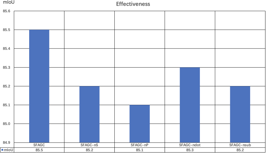
V-C Ablation Study
We also perform extra 3D point cloud segmentation experiments to validate the effectiveness of the components in the SFAGC.
The hyperparameters are the same as those shown in Table III. Here, we use some AGCs with different settings as follows:
-
1.
SFAGC. This is the full SFAGC described in Section III.
-
2.
SFAGC-nS. To validate the effectiveness of the local structure projection aggregation and fusing part proposed in the Section III-A, we discard this part from the SFAGC.
-
3.
SFAGC-nP. To confirm the effectiveness of the position embedding proposed in Section III-B, we bypass the position embedding part from the SFAGC.
-
4.
SFAGC-ndot and SFAGC-nsub. To validate the effectiveness of the multi-type attention function proposed in Section III-C, SFAGC-ndot is set as the SFAGC without the dot-production attention function, and SFAGC-nsub is set as the SFAGC without the subtraction attention function.
The architecture of the network and hyperparameters are the same as the previous experiment.
The results are summarized in Fig. 10. By comparing SFAGC with SFAGC-nS, use of the local structures in feature space increases 0.3 mIoU. In SFAGC vs. SFAGC-nP, the position-embedding phase increases 0.4 mIoU. In SFAGC vs. SFAGC-ndot, the multi-type attention function increases 0.2 mIoU. In SFAGC vs. SFAGC-nsub, the multi-type attention function increases 0.3 mIoU. The effectiveness of the SFAGC modules was demonstrated in this study.
VI Conclusion
In this paper, we propose a new attention-based graph convolution named SFAGC. It can better aggregate the structural information of the neighboring nodes in high-dimensional feature space by using local structure projection aggregation. It also can computes better attention weights by using multi-type attention functions simultaneously. Through experiments on point cloud classification and segmentation, our method outperforms existing methods.
References
- [1] J. Bruna, W. Zaremba, A. Szlam, A. Szlam, and Y. LeCun, “Spectral networks and locally connected networks on graphs,” arXiv preprint arXiv:1312.6203, 2013.
- [2] A. Karpathy, G. Toderici, S. Shetty, T. Leung, R. Sukthankar, and L. Fei-Fei, “Large-scale video classification with convolutional neural networks,” in Proceedings of the IEEE conference on Computer Vision and Pattern Recognition, 2014, pp. 1725–1732.
- [3] J. Redmon, S. Divvala, R. Girshick, and A. Farhadi, “You only look once: Unified, real-time object detection,” in Proceedings of the IEEE conference on computer vision and pattern recognition, 2016, pp. 779–788.
- [4] Z. Wu, S. Pan, F. Chen, G. Long, C. Zhang, and S. Y. Philip, “A comprehensive survey on graph neural networks,” IEEE Transactions on Neural Networks and Learning Systems, 2020.
- [5] J. Zhou, G. Cui, S. Hu, Z. Zhang, C. Yang, Z. Liu, L. Wang, C. Li, and M. Sun, “Graph neural networks: A review of methods and applications,” AI Open, vol. 1, pp. 57–81, 2020.
- [6] W. L. Hamilton, R. Ying, and J. Leskovec, “Representation learning on graphs: Methods and applications,” arXiv preprint arXiv:1709.05584, 2017.
- [7] P. W. Battaglia, J. B. Hamrick, V. Bapst, A. Sanchez-Gonzalez, V. Zambaldi, M. Malinowski, A. Tacchetti, D. Raposo, A. Santoro, R. Faulkner et al., “Relational inductive biases, deep learning, and graph networks,” arXiv preprint arXiv:1806.01261, 2018.
- [8] D. I. Shuman, S. K. Narang, P. Frossard, A. Ortega, and P. Vandergheynst, “The emerging field of signal processing on graphs: Extending high-dimensional data analysis to networks and other irregular domains,” IEEE Signal Processing Magazine, vol. 30, no. 3, pp. 83–98, 2013.
- [9] G. Cheung, E. Magli, Y. Tanaka, and M. K. Ng, “Graph spectral image processing,” Proceedings of the IEEE, vol. 106, no. 5, pp. 907–930, 2018.
- [10] M. Defferrard, X. Bresson, and P. Vandergheynst, “Convolutional neural networks on graphs with fast localized spectral filtering,” Advances in Neural Information Processing Systems, vol. 29, pp. 3844–3852, 2016.
- [11] R. Levie, F. Monti, X. Bresson, and M. M. Bronstein, “Cayleynets: Graph convolutional neural networks with complex rational spectral filters,” IEEE Transactions on Signal Processing, vol. 67, no. 1, pp. 97–109, 2018.
- [12] T. N. Kipf and M. Welling, “Semi-supervised classification with graph convolutional networks,” arXiv preprint arXiv:1609.02907, 2016.
- [13] W. Hamilton, Z. Ying, and J. Leskovec, “Inductive representation learning on large graphs,” in Advances in Neural Information Processing Systems, 2017, pp. 1024–1034.
- [14] Q. Li, Z. Han, and X.-M. Wu, “Deeper insights into graph convolutional networks for semi-supervised learning,” in Thirty-Second AAAI conference on artificial intelligence, 2018.
- [15] K. Xu, W. Hu, J. Leskovec, and S. Jegelka, “How powerful are graph neural networks?” arXiv preprint arXiv:1810.00826, 2018.
- [16] P. Veličković, G. Cucurull, A. Casanova, A. Romero, P. Lio, and Y. Bengio, “Graph attention networks,” arXiv preprint arXiv:1710.10903, 2017.
- [17] Z. Wu, S. Song, A. Khosla, F. Yu, L. Zhang, X. Tang, and J. Xiao, “3d shapenets: A deep representation for volumetric shapes,” in Proceedings of the IEEE CVPR, 2015, pp. 1912–1920.
- [18] A. X. Chang, T. Funkhouser, L. Guibas, P. Hanrahan, Q. Huang, Z. Li, S. Savarese, M. Savva, S. Song, H. Su et al., “Shapenet: An information-rich 3d model repository,” arXiv preprint arXiv:1512.03012, 2015.
- [19] F. R. Chung, Spectral graph theory. American Mathematical Soc., 1997, no. 92.
- [20] D. K. Hammond, P. Vandergheynst, and R. Gribonval, “Wavelets on graphs via spectral graph theory,” Applied and Computational Harmonic Analysis, vol. 30, no. 2, pp. 129–150, 2011.
- [21] Y. Li and Y. Tanaka, “Structural features in feature space for structure-aware graph convolution,” in 2021 IEEE International Conference on Image Processing (ICIP), 2021, pp. 3158–3162.
- [22] Y. Li and Y. Tanaka, “Structure-aware multi-hop graph convolution for graph neural networks,” IEEE Access, vol. 10, pp. 16 624–16 633, 2022.
- [23] A. Vaswani, N. Shazeer, N. Parmar, J. Uszkoreit, L. Jones, A. N. Gomez, Ł. Kaiser, and I. Polosukhin, “Attention is all you need,” Advances in neural information processing systems, vol. 30, 2017.
- [24] H. Zhao, J. Jia, and V. Koltun, “Exploring self-attention for image recognition,” in Proceedings of the IEEE CVPR, 2020, pp. 10 076–10 085.
- [25] H. Zhao, L. Jiang, J. Jia, P. H. Torr, and V. Koltun, “Point transformer,” in Proceedings of the IEEE ICCV, 2021, pp. 16 259–16 268.
- [26] C. R. Qi, H. Su, K. Mo, and L. J. Guibas, “Pointnet: Deep learning on point sets for 3d classification and segmentation,” in Proceedings of the IEEE CVPR, 2017, pp. 652–660.
- [27] Y. Wang, Y. Sun, Z. Liu, S. E. Sarma, M. M. Bronstein, and J. M. Solomon, “Dynamic graph cnn for learning on point clouds,” ACM Transactions On Graphics, vol. 38, no. 5, pp. 1–12, 2019.
- [28] M. Simonovsky and N. Komodakis, “Dynamic edge-conditioned filters in convolutional neural networks on graphs,” in Proceedings of the IEEE CVPR, 2017, pp. 3693–3702.
- [29] C. R. Qi, L. Yi, H. Su, and L. J. Guibas, “Pointnet++: Deep hierarchical feature learning on point sets in a metric space,” Advances in Neural Information Processing Systems, vol. 30, pp. 5099–5108, 2017.
- [30] J. Yang, D. Zhan, and X. Li, “Bottom-up and top-down graph pooling,” in PAKDD. Springer, 2020, pp. 568–579.
- [31] Y. Tanaka, Y. C. Eldar, A. Ortega, and G. Cheung, “Sampling signals on graphs: From theory to applications,” IEEE Signal Processing Magazine, vol. 37, no. 6, pp. 14–30, 2020.
- [32] Z. Ying, J. You, C. Morris, X. Ren, W. Hamilton, and J. Leskovec, “Hierarchical graph representation learning with differentiable pooling,” in Advances in Neural Information Processing Systems, 2018, pp. 4800–4810.
- [33] H. Gao and S. Ji, “Graph u-nets,” in ICML. PMLR, 2019, pp. 2083–2092.
- [34] J. Huang, Z. Li, N. Li, S. Liu, and G. Li, “Attpool: Towards hierarchical feature representation in graph convolutional networks via attention mechanism,” in Proceedings of the IEEE/CVF international conference on computer vision, 2019, pp. 6480–6489.
- [35] S. Xie, R. Girshick, P. Dollár, Z. Tu, and K. He, “Aggregated residual transformations for deep neural networks,” in Proceedings of the IEEE CVPR, 2017, pp. 1492–1500.
- [36] A. Newell, K. Yang, and J. Deng, “Stacked hourglass networks for human pose estimation,” in European conference on computer vision. Springer, 2016, pp. 483–499.
- [37] X. Yan, C. Zheng, Z. Li, S. Wang, and S. Cui, “Pointasnl: Robust point clouds processing using nonlocal neural networks with adaptive sampling,” in Proceedings of the IEEE/CVF Conference on Computer Vision and Pattern Recognition, 2020, pp. 5589–5598.
- [38] Y. Duan, Y. Zheng, J. Lu, J. Zhou, and Q. Tian, “Structural relational reasoning of point clouds,” in Proceedings of the IEEE/CVF Conference on Computer Vision and Pattern Recognition, 2019, pp. 949–958.
- [39] M. Guo, J. Cai, Z. Liu, T. Mu, R. R. Martin, and S. Hu, “Pct: Point cloud transformer,” Computational Visual Media, vol. 7, no. 2, pp. 187–199, 2021.
- [40] W. Wu, Z. Qi, and F. Li, “Pointconv: Deep convolutional networks on 3d point clouds,” in Proceedings of the IEEE/CVF Conference on Computer Vision and Pattern Recognition, 2019, pp. 9621–9630.
- [41] A. Komarichev, Z. Zhong, and J. Hua, “A-cnn: Annularly convolutional neural networks on point clouds,” in Proceedings of the IEEE/CVF Conference on Computer Vision and Pattern Recognition, 2019, pp. 7421–7430.
- [42] Y. Rao, J. Lu, and J. Zhou, “Spherical fractal convolutional neural networks for point cloud recognition,” in Proceedings of the IEEE/CVF Conference on Computer Vision and Pattern Recognition, 2019, pp. 452–460.
- [43] J. Mao, X. Wang, and H. Li, “Interpolated convolutional networks for 3d point cloud understanding,” in Proceedings of the IEEE/CVF International Conference on Computer Vision, 2019, pp. 1578–1587.
- [44] A. Boulch, “Convpoint: Continuous convolutions for point cloud processing,” Computers & Graphics, vol. 88, pp. 24–34, 2020.
- [45] J. Liu, B. Ni, C. Li, J. Yang, and Q. Tian, “Dynamic points agglomeration for hierarchical point sets learning,” in Proceedings of the IEEE ICCV, 2019, pp. 7546–7555.
- [46] G. Te, W. Hu, A. Zheng, and Z. Guo, “Rgcnn: Regularized graph cnn for point cloud segmentation,” in Proceedings of the ACM Multimedia, 2018, pp. 746–754.
- [47] G. Pan, J. Wang, R. Ying, and P. Liu, “3dti-net: Learn inner transform invariant 3d geometry features using dynamic gcn,” arXiv preprint arXiv:1812.06254, 2018.
- [48] Y. Zhang and M. Rabbat, “A graph-cnn for 3d point cloud classification,” in Proceedings of the IEEE ICASSP, 2018, pp. 6279–6283.
- [49] C. Wang, B. Samari, and K. Siddiqi, “Local spectral graph convolution for point set feature learning,” in Proceedings of the ECCV, 2018, pp. 52–66.
- [50] Y. Shen, C. Feng, Y. Yang, and D. Tian, “Mining point cloud local structures by kernel correlation and graph pooling,” in Proceedings of the IEEE CVPR, 2018, pp. 4548–4557.
- [51] K. Zhang, M. Hao, J. Wang, C. W. de Silva, and C. Fu, “Linked dynamic graph cnn: Learning on point cloud via linking hierarchical features,” arXiv preprint arXiv:1904.10014, 2019.
- [52] K. Hassani and M. Haley, “Unsupervised multi-task feature learning on point clouds,” in Proceedings of the IEEE ICCV, 2019, pp. 8160–8171.
- [53] C. Chen, G. Li, R. Xu, T. Chen, M. Wang, and L. Lin, “Clusternet: Deep hierarchical cluster network with rigorously rotation-invariant representation for point cloud analysis,” in Proceedings of the IEEE CVPR, 2019, pp. 4994–5002.
- [54] Q. Xu, X. Sun, C. Wu, P. Wang, and U. Neumann, “Grid-gcn for fast and scalable point cloud learning,” in Proceedings of the IEEE CVPR, 2020, pp. 5661–5670.