This paper was converted on www.awesomepapers.org from LaTeX by an anonymous user.
Want to know more? Visit the Converter page.

\PaperNumber

XX-XXX

Attitude Control of Spacecraft Formations subject to Distributed Communication Delays

Siddharth Nair Undergraduate, Department of Aerospace Engineering, Indian Institute of Technology, Bombay, 400076. This work was performed as part of an internship at the Aerospace Systems Laboratory in UT Arlington in Summer 2016       Kamesh Subbarao AAS Senior Member, Associate Professor, Department of Mechanical & Aerospace Engineering, The University of Texas at Arlington, 19018
Abstract

This paper considers the problem of achieving attitude consensus in spacecraft formations with bounded, time-varying communication delays between spacecraft connected as specified by a strongly connected topology. A state feedback controller is proposed and investigated using a time domain approach (via LMIs) and a frequency domain approach (via the small-gain theorem) to obtain delay dependent stability criteria to achieve the desired consensus. Simulations are presented to demonstrate the application of the strategy in a specific scenario.

1 Introduction

The consensus problem of multi-agent systems has been receiving significant attention in the recent years.[1, 2]. Coordination between multiple agents opens avenues for spacecraft applications such as formation control[3, 4, 5], attitude alignment[6], rendezvous[7] etc.

A set of dynamical systems is said to be synchronized when there is a complete match of configuration variables describing each system. Synchronization when pertaining to a spacecraft formation refers to the state when all the spacecraft possess a common attitude. [8] formulates the spacecraft formation problem in a Lagrangian framework and proposes a decentralized tracking law to achieve synchronization. [3] proposes a leader-follower configuration and solves the synchronization problem by designing a control strategy to make all the spacecraft track the leader(reference) spacecraft. [6] solves the attitude synchronization problem for a wider class of communication topologies (directed graphs).

In practical applications, the flow of information between spacecraft is delayed. This is often attributed to the delay in receiving data from the other spacecraft or processing of data. [9] considers the problem of synchronization of a spacecraft formation subject to constant communication delays and solves the same by using feedback linearization to track a reference trajactory while  [10] approaches the problem by proposing a backstepping controller that tracks a virtual angular velocity to achieve synchronization. [11] proposes a decentralized control approach for the same problem by appealing to the geometric structure of the configuration space of the spacecraft formation. Time-varying communication delays are considered in [12] along with delays in self-tracking control parts. This renders the dynamics nonlinear and the authors resort to constructing linear filters to derive an output feedback law.

This paper considers a spacecraft formation problem wherein there are asymmetric, bounded and time-varying delays in the communication links between the spacecraft while the feedback from the spacecraft’s own states is instantaneous. To the best of our knowledge, this problem hasn’t been attempted before and we propose a solution by linearizing the dynamics of the spacecraft formation system using the fact that the feedback is instantaneous. A controller is proposed for the delayed linear system to achieve consensus, followed by stability analysis of the system using both time domain and frequency domain approaches. Simulations at the end show the results of using the proposed controller in a formation containing four spacecraft.

2 Problem Formulation

2.1 Modified Rodrigues Parameters

The multiple spacecraft attitude consensus problem is considered with the states of each spacecraft being the Modified Rodrigues Parameters (MRP) 𝝈{\bm{\sigma}} and angular velocity 𝝎{\bm{\omega}} in the body frame. The attitude kinematics and the dynamics is assumed to be identical for all spacecraft in formation and is governed by the following nonlinear ordinary differential equations:

𝝈˙(t)\displaystyle\dot{\bm{\sigma}}(t) =\displaystyle= 𝑷(𝝈)𝝎(t)\displaystyle{\bm{P}}({\bm{\sigma}}){\bm{\omega}}(t) (1)
𝝎˙(t)\displaystyle\dot{\bm{\omega}}(t) =\displaystyle= 𝑱1([𝝎~(t)]𝑱𝝎(t)+𝝉)\displaystyle{\bm{J}}^{-1}\left(-[\tilde{\bm{\omega}}(t)]{\bm{J}}{\bm{\omega}}(t)+{\bm{\tau}}\right) (2)

where 𝑷(𝝈)=14(2[𝝈~(t)]+2𝝈(t)𝝈T(t)+(1𝝈T(t)𝝈(t))𝕀3×3){\bm{P}}({\bm{\sigma}})=\dfrac{1}{4}\left(2[\tilde{\bm{\sigma}}(t)]+2{\bm{\sigma}}(t){\bm{\sigma}}^{T}(t)+(1-{\bm{\sigma}}^{T}(t){\bm{\sigma}}(t))\mathbb{I}_{3\times 3}\right), [𝒂~]=[0a3a2a30a1a2a10][\tilde{\bm{a}}]=\begin{bmatrix}0&-a_{3}&a_{2}\\ a_{3}&0&-a_{1}\\ -a_{2}&a_{1}&0\end{bmatrix},

𝑱{\bm{J}} is the symmetric moment of Inertia matrix and 𝝉{\bm{\tau}} is the control torque.

The MRP is a vector defined as

𝝈=𝒏^tan(Φ4){\bm{\sigma}}=\hat{\bm{n}}\tan\left(\frac{\Phi}{4}\right)

where 𝒏^\hat{\bm{n}} is the principal axis and Φ\Phi is the principal angle as given by Euler’s rotation theorem. The MRPs yield a unique representation for the attitude of the spacecraft for all principal rotations that lie in the interval [0,2π)[0,~2\pi). At Φ=2π\Phi=2\pi, a singularity is encountered that is typically addressed using the shadow MRP set. In this paper, it is assumed that the rotations are limited to principal rotation angles less than 2π2\pi.

2.2 Feedback Linearization

The system represented by Eqs. (1) and (2) is rewritten into a compact second order nonlinear ode:

𝑴(𝝈)𝝈¨+𝑪(𝝈,𝝈˙)𝝈˙=𝒖{\bm{M}}({\bm{\sigma}})\ddot{\bm{\sigma}}+{\bm{C}}({\bm{\sigma}},\dot{\bm{\sigma}})\dot{\bm{\sigma}}={\bm{u}} (3)

Let 𝝈1=𝝈{\bm{\sigma}}_{1}={\bm{\sigma}} and 𝝈2=𝝈˙{\bm{\sigma}}_{2}=\dot{\bm{\sigma}}. Performing the transformations 𝝎=𝑷(𝝈)1𝝈˙{\bm{\omega}}={\bm{P}}({\bm{\sigma}})^{-1}\dot{\bm{\sigma}} and 𝑷(𝝈)1𝝉=𝒖{\bm{P}}({\bm{\sigma}})^{-1}{\bm{\tau}}={\bm{u}} the dynamics can be expressed as

𝝈˙1\displaystyle\dot{\bm{\sigma}}_{1} =𝝈2\displaystyle={\bm{\sigma}}_{2}
𝝈˙2\displaystyle\dot{\bm{\sigma}}_{2} =𝑴(𝝈1)1(𝑪(𝝈1,𝝈2)𝝈2+𝒖)\displaystyle={\bm{M}}({\bm{\sigma}}_{1})^{-1}\left(-{\bm{C}}({\bm{\sigma}}_{1},{\bm{\sigma}}_{2}){\bm{\sigma}}_{2}+{\bm{u}}\right) (4)

where 𝑴(𝝈1)=𝑷(𝝈1)1𝑱𝑷(𝝈1){\bm{M}}({\bm{\sigma}}_{1})={\bm{P}}({\bm{\sigma}}_{1})^{-1}{\bm{J}}{\bm{P}}({\bm{\sigma}}_{1}) and 𝑪(𝝈1,𝝈2)=𝑷(𝝈1)1(𝑱𝑷˙(𝝈1)+[𝑷(𝝈1)𝝈2]~𝑱𝑷(𝝈1)){\bm{C}}({\bm{\sigma}}_{1},{\bm{\sigma}}_{2})={\bm{P}}({\bm{\sigma}}_{1})^{-1}\left({\bm{J}}\dot{\bm{P}}({\bm{\sigma}}_{1})+\widetilde{\left[{\bm{P}}({\bm{\sigma}}_{1}){\bm{\sigma}}_{2}\right]}{\bm{J}}{\bm{P}}({\bm{\sigma}}_{1})\right).

Using full state feedback and a straightforward feedback linearization based control law, 𝒖=𝑪(𝝈1,𝝈2)𝝈2+𝑴(𝝈1)𝒗{\bm{u}}={\bm{C}}({\bm{\sigma}}_{1},{\bm{\sigma}}_{2}){\bm{\sigma}}_{2}+{\bm{M}}({\bm{\sigma}}_{1}){\bm{v}}, the above dynamics are further reduced to that of a double integrator as follows.

𝝈˙1\displaystyle\dot{\bm{\sigma}}_{1} =𝝈2\displaystyle={\bm{\sigma}}_{2}
𝝈˙2\displaystyle\dot{\bm{\sigma}}_{2} =𝒗\displaystyle={\bm{v}} (5)

2.3 Consensus of Spacecraft Formation

Now, consider a system of NN spacecraft with communication pathways among them forming a strongly connected graph, each of whom is being controlled using the control law 𝒖(t){\bm{u}}(t) described earlier. Thus, the attitude consensus problem for NN nonlinear spacecraft can be posed using the simpler structure derived earlier in Eq. (5).

Let 𝐱=[𝐱𝟏T𝐱𝟐T]T\mathbf{x}=[\mathbf{x_{1}}^{T}\ \mathbf{x_{2}}^{T}]^{T} be a vector such 𝐱1\mathbf{x}_{1} consists of the attitudes of the NN spacecraft while 𝐱𝟐\mathbf{x_{2}} consists of their derivatives i.e. 𝐱𝟏=[𝝈1T1𝝈1TN]T\mathbf{x_{1}}=\left[{}^{1}{\bm{\sigma}}_{1}^{T}\cdots{}^{N}{\bm{\sigma}}_{1}^{T}\right]^{T} and 𝐱𝟐=[𝝈2T1𝝈2TN]T\mathbf{x_{2}}=\left[{}^{1}{\bm{\sigma}}_{2}^{T}\cdots{}^{N}{\bm{\sigma}}_{2}^{T}\right]^{T}. This vector defines the state of the NN spacecraft system and the combined dynamics can be written as:

𝐱˙𝟏(t)\displaystyle\mathbf{\dot{x}_{1}}(t) =𝐱𝟐(t)\displaystyle=\mathbf{x_{2}}(t)
𝐱˙𝟐(t)\displaystyle\mathbf{\dot{x}_{2}}(t) =𝐮(t)\displaystyle={\mathbf{u}}(t) (6)

where the vector 𝐮=[𝒗T1𝒗TN]T{\mathbf{u}}=\left[{}^{1}{\bm{v}}^{T}\cdots{}^{N}{\bm{v}}^{T}\right]^{T} is the control input obtained by cascading the control inputs of all the spacecraft.

For the system of NN spacecraft described above in Eq. (2.3), attitude consensus is said to be achieved when 𝝈1i𝝈1j0||{}^{i}{\bm{\sigma}}_{1}-{}^{j}{\bm{\sigma}}_{1}||\rightarrow 0 and 𝝈2i𝝈2j0||{}^{i}{\bm{\sigma}}_{2}-{}^{j}{\bm{\sigma}}_{2}||\rightarrow 0 as tt\rightarrow\infty i,j,ij\forall\ i,~j,~i\neq j.

In the case where the spacecraft exchange state information to their connected neighbors with no delay, the following control law drives the system to consensus [13]. For all the analysis from here on, we will use the compact set of equations in Eq. (2.3) for the NN connected spacecraft.

𝐮(t)=𝐋𝐱𝟏(t)γ𝐋𝐱𝟐(t)\mathbf{u}(t)=-\mathbf{L}\mathbf{x_{1}}(t)-\gamma\mathbf{L}\mathbf{x_{2}}(t)

where 𝐋=[lij]\mathbf{L}=[l_{ij}] is the Laplacian matrix for a given communication topology [5, 13] and γ>0\gamma>0 is a damping gain.

2.4 Proposed Control Law

In this paper, the consensus problem is analyzed when the communication is subject to time delays i.e. the state information of the ithi^{\mathrm{th}} spacecraft is relayed to the jthj^{\mathrm{th}} spacecraft after a delay τij\tau_{ij} that satisfies

0τijhij&|τ˙ij|dij\displaystyle 0~\leq~\tau_{ij}~\leq~h_{ij}\quad\&\quad|\dot{\tau}_{ij}|~\leq~d_{ij} (7)

Clearly the time delays are different along different communication paths (spacecraft pairs) and are time-varying.

To achieve consensus, the following control law is investigated.

𝐮(t)=𝐱𝟏(t)γ𝐱𝟐(t)i=1Nj=1Nij𝐊𝐱𝟏ij(tτij)i=1Nj=1Nijγ𝐊𝐱𝟐ij(tτij)\displaystyle\mathbf{u}(t)=-\mathbf{x_{1}}(t)-\gamma\mathbf{x_{2}}(t)-\mathop{\sum_{i=1}^{N}\sum_{j=1}^{N}}_{i\neq j}{}^{ij}\mathbf{K}\mathbf{x_{1}}(t-\tau_{ij})-\mathop{\sum_{i=1}^{N}\sum_{j=1}^{N}}_{i\neq j}\gamma{}^{ij}\mathbf{K}\mathbf{x_{2}}(t-\tau_{ij}) (8)

For NN spacecraft defining the communication topology, then for every pair (i,j)(i,~j) of spacecraft we have lij0l_{ij}\leq 0 (from the Laplacian matrix). 𝐊ijN×N{}^{ij}\mathbf{K}\in\mathbb{R}^{N\times N} and 𝐊ij𝕀3×3{}^{ij}\mathbf{K}\otimes\mathbb{I}_{3\times 3} is the coefficient of the delayed state, where τij\tau_{ij} is the time delay in sending information from the ithi^{\mathrm{th}} spacecraft to the jthj^{\mathrm{th}} spacecraft. The jithji^{th} element of 𝐊ij{}^{ij}\mathbf{K} is equal to lijl_{ij}. All other elements are zero.
This is illustrated via an example involving three spacecraft with the communication topology specified by figure  1.

Refer to caption
Figure 1: Communication graph for the three spacecraft

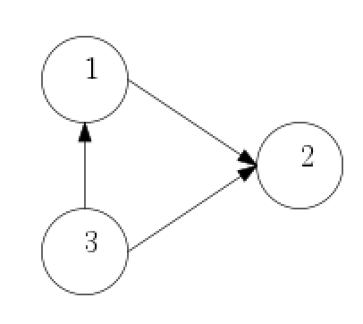
The Laplacian matrix specifying the communication topology between the three spacecraft be given by

[10112112000]\begin{bmatrix}1&0&-1\\ -\frac{1}{2}&1&-\frac{1}{2}\\ 0&0&0\end{bmatrix}

Let the delays in the communication channels be τ12,τ31\tau_{12},\ \tau_{31} and τ32\tau_{32}. Then, the matrices Kij{}^{ij}K are given by

K12=[0001200000]𝕀3×331K=[001000000]𝕀3×332K=[0000012000]𝕀3×3{}^{12}K=\begin{bmatrix}0&0&0\\ -\frac{1}{2}&0&0\\ 0&0&0\end{bmatrix}\otimes\mathbb{I}_{3\times 3}\ ^{31}K=\begin{bmatrix}0&0&-1\\ 0&0&0\\ 0&0&0\end{bmatrix}\otimes\mathbb{I}_{3\times 3}\ ^{32}K=\begin{bmatrix}0&0&0\\ 0&0&-\frac{1}{2}\\ 0&0&0\end{bmatrix}\otimes\mathbb{I}_{3\times 3}\

Substituting Eq. (8) in Eq. (2.3), the state dynamics are expressed as a linear differential equation with multiple time delays.

𝐱˙(t)=𝐀0𝐱(t)+i=1Nj=1Nij𝐀𝐱ij(tτij)\displaystyle\mathbf{\dot{x}}(t)=\mathbf{A}_{0}\mathbf{x}(t)+\mathop{\sum_{i=1}^{N}\sum_{j=1}^{N}}_{i\neq j}{}^{ij}\mathbf{A}\mathbf{x}(t-\tau_{ij}) (9)

where
𝐀0=[𝟎N×N𝕀N×N𝕀N×Nγ𝕀N×N]𝕀3×3\mathbf{A}_{0}=\begin{bmatrix}\mathbf{0}_{N\times N}&\mathbb{I}_{N\times N}\\ -\mathbb{I}_{N\times N}&-\gamma\mathbb{I}_{N\times N}\end{bmatrix}\otimes\mathbb{I}_{3\times 3}  and  𝐀ij=[𝟎N×N𝟎N×N𝐊ijγ𝐊ij]𝕀3×3{}^{ij}\mathbf{A}=\begin{bmatrix}\mathbf{0}_{N\times N}&\mathbf{0}_{N\times N}\\ -{}^{ij}\mathbf{K}&-\gamma{}^{ij}\mathbf{K}\end{bmatrix}\otimes\mathbb{I}_{3\times 3}.

Note that i=1Nj=1Nij𝐀ij=[𝟎N×N𝟎N×N𝒜γ𝒜]𝕀3×3=𝐀γ\mathop{\sum_{i=1}^{N}\sum_{j=1}^{N}}_{i\neq j}{}^{ij}\mathbf{A}=\begin{bmatrix}\mathbf{0}_{N\times N}&\mathbf{0}_{N\times N}\\ \mathcal{A}&\gamma\mathcal{A}\end{bmatrix}\otimes\mathbb{I}_{3\times 3}=\mathbf{A}_{\gamma} where 𝒜\mathcal{A} is the adjacency matrix of the connection topology.

3 Stability Analysis

3.1 Time Domain Approach

Lemma 1 (Schur’s Complement [14])

The following linear matrix inequality (LMI)

𝐒=[𝐒𝟏𝟏𝐒𝟏𝟐𝐒𝟐𝟏𝐒𝟐𝟐]<0\mathbf{S}=\begin{bmatrix}\mathbf{S_{11}}&\mathbf{S_{12}}\\ \mathbf{S_{21}}&\mathbf{S_{22}}\end{bmatrix}<0

where 𝐒=𝐒T\mathbf{S}=\mathbf{S}^{T}, is equivalent to each of the following conditions:

𝐒𝟏𝟏<0,𝐒𝟐𝟐𝐒𝟏𝟐T𝐒𝟏𝟏1𝐒𝟏𝟐<0,\mathbf{S_{11}}<0,\ \mathbf{S_{22}}-\mathbf{S_{12}}^{T}\mathbf{S_{11}}^{-1}\mathbf{S_{12}}<0,
𝐒𝟐𝟐<0,𝐒𝟏𝟏𝐒𝟏𝟐𝐒𝟐𝟐1𝐒𝟏𝟐T<0\mathbf{S_{22}}<0,\ \mathbf{S_{11}}-\mathbf{S_{12}}\mathbf{S_{22}}^{-1}\mathbf{S_{12}}^{T}<0
Lemma 2 (Jensen’s Inequality [14])

For any constant matrix Pm×mP\in\mathbb{R}^{m\times m}, P=PT>0P=P^{T}>0, scalar γ>0\gamma>0, vector function ω:[0,γ]m\omega:[0,\gamma]\rightarrow\mathbb{R}^{m} such that the integrations concerned are well defined, then

γ0γωT(β)Pω(β)𝑑β(0γω(β)𝑑β)TP(0γω(β)𝑑β)\gamma\int_{0}^{\gamma}\omega^{T}(\beta)P\omega(\beta)d\beta\geq\left(\int_{0}^{\gamma}\omega(\beta)d\beta\right)^{T}P\left(\int_{0}^{\gamma}\omega(\beta)d\beta\right)

The lemmas stated above are key to obtaining an LMI condition for ensuring stability of the desired consensus.

Theorem 1

Under the action of (8), the solutions to the dynamics given by (2.3) converge to consensus if there exist symmetric, positive definite matrices Qij6(n1)×6(n1)Q_{ij}\in\mathbb{R}^{6(n-1)\times 6(n-1)}, Sij6(n1)×6(n1)S_{ij}\in\mathbb{R}^{6(n-1)\times 6(n-1)} and positive constant γ\gamma such that the following LMIs hold

Ψ1\displaystyle\Psi_{1} <𝟎\displaystyle<\mathbf{0}
Ψ2\displaystyle\Psi_{2} <𝟎\displaystyle<\mathbf{0}
Ψ3\displaystyle\Psi_{3} <𝟎\displaystyle<\mathbf{0}

where

Ψ1=[ETEA0+A0TETEETEA12ETEA13ETEAnn1A12TETE000A13TETE000Ann1TETE000]\Psi_{1}=\begin{bmatrix}E^{T}EA_{0}+A^{T}_{0}E^{T}E&E^{T}EA_{12}&E^{T}EA_{13}&\ldots&E^{T}EA_{nn-1}\\ A^{T}_{12}E^{T}E&0&0&\ldots&0\\ A^{T}_{13}E^{T}E&0&0&\ldots&0\\ \vdots&\vdots&\vdots&\ddots&\vdots\\ A^{T}_{nn-1}E^{T}E&0&0&\ldots&0\end{bmatrix}
Ψ2=[i=1nj=1nijETQijE000ETQ12E00ETQnn1E]\Psi_{2}=\begin{bmatrix}\mathop{\sum_{i=1}^{n}\sum_{j=1}^{n}}_{i\neq j}E^{T}Q_{ij}E&0&\ldots&0\\ 0&-E^{T}Q_{12}E&\vdots&\vdots\\ \vdots&0&\ddots&\vdots\\ 0&\ldots&&-E^{T}Q_{nn-1}E\end{bmatrix}
Ψ3=[Ψ11Ψ12Ψ1nA0TETΨ12TΨ23A12TETΨ1nTΨnn1Ann1TETEA0EA12EAnn1(i=1nj=1nijhijSij)1]\Psi_{3}=\begin{bmatrix}\Psi_{11}&\Psi_{12}&\ldots&\Psi_{1n}&A^{T}_{0}E^{T}\\ \Psi_{12}^{T}&\ddots&\Psi_{23}\ldots&\vdots&A^{T}_{12}E^{T}\\ \vdots&\vdots&\ddots&\vdots&\vdots\\ \Psi_{1n}^{T}&\ldots&\ldots&\Psi_{nn-1}&A^{T}_{n\ n-1}E^{T}\\ EA_{0}&EA_{12}&\ddots&EA_{n\ n-1}&-(\mathop{\sum_{i=1}^{n}\sum_{j=1}^{n}}_{i\neq j}h_{ij}S_{ij})^{-1}\end{bmatrix}

where

E\displaystyle E =[[𝟏𝕀n1]𝟎𝟎[𝟏𝕀n1]]𝕀3×3\displaystyle=\begin{bmatrix}\left[\mathbf{1}\ -\mathbb{I}_{n-1}\right]&\mathbf{0}\\ \mathbf{0}&\left[\mathbf{1}\ -\mathbb{I}_{n-1}\right]\end{bmatrix}\otimes\mathbb{I}_{3\times 3}
Ψ11\displaystyle\Psi_{11} =i=1nj=1nij(1dijhijET(Sij)E)\displaystyle=\mathop{\sum_{i=1}^{n}\sum_{j=1}^{n}}_{i\neq j}(\frac{1-d_{ij}}{h_{ij}}E^{T}(S_{ij})E)
Ψ12\displaystyle\Psi_{12} =(1d12h12ET(S12)E)\displaystyle=(\frac{1-d_{12}}{h_{12}}E^{T}(S_{12})E)
Ψ22\displaystyle\Psi_{22} =(1d12h12ET(S12)E)\displaystyle=(-\frac{1-d_{12}}{h_{12}}E^{T}(S_{12})E)
Ψ23\displaystyle\Psi_{23} =𝟎\displaystyle=\mathbf{0}
..and so on.\displaystyle..\textrm{and so on.}

Proof
Consider the following Lyapunov-Krasovskii candidate funtional with 𝐲(t)=E𝐱(t)(i.e.,𝐲1=[𝟏𝕀n1]𝕀3×3𝐱1,𝐲2=[𝟏𝕀n1]𝕀3×3𝐱2\mathbf{y}(t)=E\mathbf{x}(t)\ (i.e.,\mathbf{y}_{1}=\left[\mathbf{1}\ -\mathbb{I}_{n-1}\right]\otimes\mathbb{I}_{3\times 3}\ \mathbf{x}_{1},\ \mathbf{y}_{2}=\left[\mathbf{1}\ -\mathbb{I}_{n-1}\right]\otimes\mathbb{I}_{3\times 3}\ \mathbf{x}_{2})

V=\displaystyle V= 𝐲(t)T𝐲(t)V1+i=1nj=1nijtτijt𝐲(s)TQij𝐲(s)𝑑sV2\displaystyle\underbrace{\mathbf{y}(t)^{T}\mathbf{y}(t)}_{V_{1}}+\underbrace{\mathop{\sum_{i=1}^{n}\sum_{j=1}^{n}}_{i\neq j}\int_{t-\tau_{ij}}^{t}\mathbf{y}(s)^{T}Q_{ij}\mathbf{y}(s)ds}_{V_{2}}
+i=1nj=1nijtτijtηt𝐲˙(s)TSij𝐲˙(s)𝑑s𝑑ηV3\displaystyle+\underbrace{\mathop{\sum_{i=1}^{n}\sum_{j=1}^{n}}_{i\neq j}\int_{t-\tau_{ij}}^{t}\int_{\eta}^{t}\mathbf{\dot{y}}(s)^{T}S_{ij}\mathbf{\dot{y}}(s)dsd\eta}_{V_{3}}

where Qij,SijQ_{ij},S_{ij} are appropriately dimensioned symmetric positive definite matrices.
Defining 𝐗=[𝐱(t)T𝐱T(tτ12)𝐱T(tτ13)𝐱T(tτnn1)]T\mathbf{X}=[\mathbf{x}(t)^{T}\ \mathbf{x}^{T}(t-\tau_{12})\ \mathbf{x}^{T}(t-\tau_{13})...\mathbf{x}^{T}(t-\tau_{nn-1})]^{T}, the derivatives of each individual term of the Lyapunov-Krasovskii functional are obtained as

V˙1=𝐗TΨ1𝐗\dot{V}_{1}=\mathbf{X}^{T}\Psi_{1}\mathbf{X}
V˙2=𝐗TΨ2𝐗\dot{V}_{2}=\mathbf{X}^{T}\Psi_{2}\mathbf{X}
V˙3\displaystyle\dot{V}_{3} i=1nj=1nijhij𝐱˙𝐓(t)ET(Sij)L𝐱˙(t)\displaystyle\leq\mathop{\sum_{i=1}^{n}\sum_{j=1}^{n}}_{i\neq j}h_{ij}\mathbf{\dot{x}^{T}}(t)E^{T}(S_{ij})L\mathbf{\dot{x}}(t)
i=1nj=1nij(1dij)tτijt𝐱˙𝐓(s)ET(Sij)L𝐱˙(s)𝑑s\displaystyle-\mathop{\sum_{i=1}^{n}\sum_{j=1}^{n}}_{i\neq j}(1-d_{ij})\int_{t-\tau_{ij}}^{t}\mathbf{\dot{x}^{T}}(s)E^{T}(S_{ij})L\mathbf{\dot{x}}(s)ds

Using Jensen’s inequality (Lemma 2), the above inequality can be expressed as

V˙3\displaystyle\dot{V}_{3} 𝐗TΩ𝐗\displaystyle\leq\mathbf{X}^{T}\Omega\mathbf{X}

where

Ω=[Ω11Ω12Ω1nΩ12TΩ23Ω1nTΩnn1]\Omega=\begin{bmatrix}\Omega_{11}&\Omega_{12}&\ldots&\Omega_{1n}\\ \Omega_{12}^{T}&\ddots&\Omega_{23}\ldots&\vdots\\ \vdots&\vdots&\ddots&\vdots\\ \Omega_{1n}^{T}&\ldots&\ldots&\Omega_{nn-1}\end{bmatrix}

and

Ω11\displaystyle\Omega_{11} =i=1nj=1nij(hijA0TET(Sij)EA01dijhijET(Sij)E)\displaystyle=\mathop{\sum_{i=1}^{n}\sum_{j=1}^{n}}_{i\neq j}(h_{ij}A^{T}_{0}E^{T}(S_{ij})EA_{0}-\frac{1-d_{ij}}{h_{ij}}E^{T}(S_{ij})E)
Ω12\displaystyle\Omega_{12} =i=1nj=1nijhijA0TET(Sij)EA12+1d12h12ET(S12)E\displaystyle=\mathop{\sum_{i=1}^{n}\sum_{j=1}^{n}}_{i\neq j}h_{ij}A^{T}_{0}E^{T}(S_{ij})EA_{12}+\frac{1-d_{12}}{h_{12}}E^{T}(S_{12})E
Ω22\displaystyle\Omega_{22} =i=1nj=1nijhijA12TET(Sij)EA121d12h12ET(S12)E\displaystyle=\mathop{\sum_{i=1}^{n}\sum_{j=1}^{n}}_{i\neq j}h_{ij}A^{T}_{12}E^{T}(S_{ij})EA_{12}-\frac{1-d_{12}}{h_{12}}E^{T}(S_{12})E
Ω23\displaystyle\Omega_{23} =i=1nj=1nijhijA12TET(Sij)EA13\displaystyle=\mathop{\sum_{i=1}^{n}\sum_{j=1}^{n}}_{i\neq j}h_{ij}A^{T}_{12}E^{T}(S_{ij})EA_{13}
..and so on.\displaystyle..\textrm{and so on.}

To make the elements of the above matrix affine in the unknown variables, Schur’s complement (Lemma 1) is applied using the fact that i=1nj=1nijhijSij\mathop{\sum_{i=1}^{n}\sum_{j=1}^{n}}_{i\neq j}h_{ij}S_{ij} is positive definite and invertible. The resulting LMI is Ψ3=<𝟎\Psi_{3}=<\mathbf{0}

The vector 𝐲(t)\mathbf{y}(t) converges to 𝟎\mathbf{0} if there exist symmetric positive definite matrices P,Qij,SijP,\ Q_{ij},\ S_{ij} such that the following LMIs are feasible

Ψ1\displaystyle\Psi_{1} <𝟎\displaystyle<\mathbf{0}
Ψ2\displaystyle\Psi_{2} <𝟎\displaystyle<\mathbf{0}
Ψ3\displaystyle\Psi_{3} <𝟎\displaystyle<\mathbf{0}

Observe that 𝐲𝟏𝐢(t)=𝐱𝟏𝟏(t)𝐱𝟏𝐢+𝟏(t)i>1\mathbf{y_{1i}}(t)=\mathbf{x_{11}}(t)-\mathbf{x_{1\ i+1}}(t)\ \forall\ i>1 . Thus, if 𝐲(t)𝟎\mathbf{y}(t)\rightarrow\mathbf{0} as tt\rightarrow\infty, we have 𝐱𝟏𝟏(t)=𝐱𝟏𝐢(t)\mathbf{x_{11}}(t)=\mathbf{x_{1i}}(t) as ti>1t\rightarrow\infty\ \forall\ i>1. Hence, consensus is achieved.\blacksquare
Note that finding feasible solutions for the above LMIs is a tedious task considering that the LK functional is required to be positive definite on the augmented state space 𝐲(t)\mathbf{y}(t) while its derivative is required to be negative definite on the actual state space 𝐱(t)\mathbf{x}(t) which can’t be obtained from 𝐲(t)\mathbf{y}(t) via an invertible transformation due to the nature of how the time delays appear in the closed loop dynamics. To guarantee feasible solutions, a leader-follower strategy or a constant set point must be specified to obtain an invertible transformation such that the derivatives of 𝐲(t)\mathbf{y}(t) appear as linear functions of 𝐲(t)\mathbf{y}(t) itself, i.e, 𝐘˙(t)=𝐀¯0𝐘(t)+i=1Nj=1Nij𝐀¯ij𝐘(tτij)\dot{\mathbf{Y}}(t)=\bar{\mathbf{A}}_{0}\mathbf{Y}(t)+\mathop{\sum_{i=1}^{N}\sum_{j=1}^{N}}_{i\neq j}{}^{ij}\bar{\mathbf{A}}\mathbf{Y}(t-\tau_{ij}).
To this end, we also investigate the consensus problem using a frequency domain approach to obtain delay dependent stability criteria.

Frequency Domain Approach

We adopt a frequency domain approach by making use of the small-gain theorem to show that the system achieves consensus. Before stating the main theorem, we present a few lemmas and the small-gain theorem itself.
Let L2pL^{p}_{2} be the space of p\mathbb{R}^{p} valued functions f:[0,)pf:[0,\infty)\rightarrow\mathbb{R}^{p} such that its L2L_{2} norm is bounded, i.e,

fL2=0fT(t)f(t)𝑑t<||f||_{L_{2}}=\int^{\infty}_{0}f^{T}(t)f(t)dt<\infty

Let L2epL^{p}_{2e} be an extended space containing functions that satisfy the above inequality on finite intervals. An operator is defined as a function G:L2epL2eqG:L^{p}_{2e}\rightarrow L^{q}_{2e} with an induced norm defined as

G=sup(G(f)f):fL2ep,f0||G||=sup\left(\frac{||G(f)||}{||f||}\right):\forall f\in L^{p}_{2e},f\neq 0
Refer to caption
Figure 2: Feedback System
Lemma 3 (Small-Gain theorem)
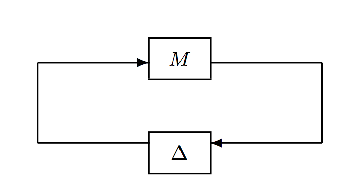
Suppose that MM and Δ\Delta are both stable systems with finite input-output gains. Let M||M|| and Δ||\Delta|| denote their respective induced norms. Then the feedback system in figure  2 is stable if

MΔ<1||M\Delta||<1

The small-gain theorem provides a sufficient condition for stability of feedback systems. Let us examine the form of  (9) more closely.

𝐱˙(t)\displaystyle\mathbf{\dot{x}}(t) =𝐀0𝐱(t)+i=1Nj=1Nij𝐀𝐱ij(tτij)\displaystyle=\mathbf{A}_{0}\mathbf{x}(t)+\mathop{\sum_{i=1}^{N}\sum_{j=1}^{N}}_{i\neq j}{}^{ij}\mathbf{A}\mathbf{x}(t-\tau_{ij})
𝐱˙(t)\displaystyle\Rightarrow\mathbf{\dot{x}}(t) =𝐀0𝐱(t)+i=1Nj=1Nij𝐀ij(𝐱(tτij)𝐱(t))+i=1Nj=1Nij𝐀𝐱ij(t)\displaystyle=\mathbf{A}_{0}\mathbf{x}(t)+\mathop{\sum_{i=1}^{N}\sum_{j=1}^{N}}_{i\neq j}{}^{ij}\mathbf{A}(\mathbf{x}(t-\tau_{ij})-\mathbf{x}(t))+\mathop{\sum_{i=1}^{N}\sum_{j=1}^{N}}_{i\neq j}{}^{ij}\mathbf{A}\mathbf{x}(t)
𝐱˙(t)\displaystyle\Rightarrow\mathbf{\dot{x}}(t) =𝐀0𝐱(t)+i=1Nj=1Nij𝐀ij(𝐱(tτij)𝐱(t))+𝐀γ𝐱(t)\displaystyle=\mathbf{A}_{0}\mathbf{x}(t)+\mathop{\sum_{i=1}^{N}\sum_{j=1}^{N}}_{i\neq j}{}^{ij}\mathbf{A}(\mathbf{x}(t-\tau_{ij})-\mathbf{x}(t))+\mathbf{A}_{\gamma}\mathbf{x}(t)
𝐱˙(t)𝐀γ𝐱(t)𝐀0𝐱(t)\displaystyle\Rightarrow\mathbf{\dot{x}}(t)-\mathbf{A}_{\gamma}\mathbf{x}(t)-\mathbf{A}_{0}\mathbf{x}(t) =i=1Nj=1Nij𝐀ij(𝐱(tτij)𝐱(t))\displaystyle=\mathop{\sum_{i=1}^{N}\sum_{j=1}^{N}}_{i\neq j}{}^{ij}\mathbf{A}(\mathbf{x}(t-\tau_{ij})-\mathbf{x}(t))

Thus, the system of spacecraft in our problem  (9) can be viewed as a feedback system with the same structure in Figure  2 with the transfer function

𝐗(s)=𝐓(s)Δ(𝐗(s))\mathbf{X}(s)=\mathbf{T}(s)\Delta(\mathbf{X}(s))

where 𝐓(s)=(s𝕀6N×6N𝐀0𝐀γ)1[𝐀12𝐀13𝐀nn1]\mathbf{T}(s)=(s\mathbb{I}_{6N\times 6N}-\mathbf{A}_{0}-\mathbf{A}_{\gamma})^{-1}\left[\mathbf{A}_{12}\ \mathbf{A}_{13}...\ \mathbf{A}_{nn-1}\right] and Δ=[Δτ12000Δτ1300..0Δτnn1]\Delta=\begin{bmatrix}\Delta_{\tau_{12}}&0&...&0\\ 0&\Delta_{\tau_{13}}&...&0\\ 0&..&0&\Delta_{\tau_{nn-1}}\end{bmatrix} with delay operators Δτ\Delta_{\tau} defined as Δτ(𝐱(t))=𝐱(t)𝐱(tτ)\Delta_{\tau}(\mathbf{x}(t))=\mathbf{x}(t)-\mathbf{x}(t-\tau)

Lemma 4[15])

Let 𝕊\mathbb{S} be a set of differentiable functions such that 𝕊={τ(t)|τ(t)[0,τ0],τ˙(t)dt}\mathbb{S}=\left\{\tau(t)|\tau(t)\in[0,\tau_{0}],\dot{\tau}(t)\leq d\ \forall t\ \right\}. Then the delay operator obeys the following equality

supτ(t)𝕊(Δτ1s)=τ0\mathop{sup}_{\tau(t)\in\mathbb{S}}(||\Delta_{\tau}\frac{1}{s}||)=\tau_{0}

Proof
Let v(t)L2epv(t)\in L^{p}_{2e}. Then

Δτ1sv(t)=tτ(t)tv(t)𝑑t\Delta_{\tau}\frac{1}{s}v(t)=\int^{t}_{t-\tau(t)}v(t)dt

Now,

Δτ1sv(t)2=(tτ(t)tv(s)𝑑s)T(tτ(t)tv(s)𝑑s)||\Delta_{\tau}\frac{1}{s}v(t)||^{2}=(\int^{t}_{t-\tau(t)}v(s)ds)^{T}(\int^{t}_{t-\tau(t)}v(s)ds)

Using lemma  2, we have

Δτ1sv(t)2τ0(tτ0tvT(s)v(s)𝑑s)||\Delta_{\tau}\frac{1}{s}v(t)||^{2}\leq\tau_{0}(\int^{t}_{t-\tau_{0}}v^{T}(s)v(s)ds)

The L2L_{2} norm of Δτ1sv(t)\Delta_{\tau}\frac{1}{s}v(t) is bounded above as follows

Δτ1sv(t)L22\displaystyle||\Delta_{\tau}\frac{1}{s}v(t)||_{L_{2}}^{2} 0τ0(tτ0tvT(s)v(s)𝑑s)𝑑t\displaystyle\leq\int^{\infty}_{0}\tau_{0}(\int^{t}_{t-\tau_{0}}v^{T}(s)v(s)ds)dt
=τ0τ000vT(s)v(s)𝑑t𝑑s\displaystyle=\tau_{0}\int^{0}_{-\tau_{0}}\int^{\infty}_{0}v^{T}(s)v(s)dtds
τ02vL2\displaystyle\leq\tau^{2}_{0}||v||_{L_{2}}

\blacksquare
The above lemma establishes a bound for the delay operator. The small-gain theorem also requires the plant 𝐓(s)\mathbf{T}(s) to be stable. The following lemma characterizes the values of the gain γ\gamma that render the system stable in the case where the delays are non-existent.

Lemma 5[13])

The system described by  (9) in the case where the delays are non-existent is stable for the values of γ\gamma which satisfy

γ>maxμi02|μi|cos(π2tan1(ReμiImμi))\gamma>\mathop{max}_{\mu_{i}\neq 0}\sqrt{\frac{2}{|\mu_{i}|\cos(\frac{\pi}{2}-tan^{-1}(\frac{-Re\ \mu_{i}}{Im\ \mu_{i}}))}}

if the connection topology of the spacecraft formation has a rooted directed spanning tree.

Now we make use of the above lemmas to prove the following theorem which establishes the condition under which consensus is guaranteed.

Theorem 2

The system of spacecraft with dynamics dictated by  (9) connected via a network topology containing a rooted directed spanning tree, achieves consensus if along with the conditions of lemmas  4 and  5, the following holds

τ0<1ωmaxμik=1pi|(jωγμi±γ2μi2+4μi2)k|(1+γ)ω(0,)\tau_{0}<\frac{1}{\omega\ \mathop{max}_{\mu_{i}}\sum^{p_{i}}_{k=1}|(j\omega-\frac{\gamma\mu_{i}\pm\sqrt{\gamma^{2}\mu^{2}_{i}+4\mu_{i}}}{2})^{-k}|(1+\gamma)}\quad\forall\omega\in(0,\infty)

where μi\mu_{i} are the eigenvalues of 𝐋𝕀3×3-\mathbf{L}\otimes\mathbb{I}_{3\times 3}, pip_{i} are the multiplicities of the corresponding eigenvalues of 𝐀0+𝐀γ\mathbf{A}_{0}+\mathbf{A}_{\gamma} and τ0=maxi,jhij\tau_{0}=\mathop{max}_{i,j}h_{ij}.

Proof
Now that we have that the individual transfer functions 𝐓(s)\mathbf{T}(s) and Δ\Delta are stable with finite input-output gains, we proceed to find a bound on 𝐓Δ||\mathbf{T}\Delta|| and subsequently use the small-gain theorem to show that consensus is achieved for all signals with frequencies ω[0,)\omega\in[0,\infty)

T(s)Δ\displaystyle||T(s)\Delta|| =(s𝕀6N×6N𝐀0𝐀γ)1[s𝐀12s𝐀13s𝐀nn1]Δ1s\displaystyle=||(s\mathbb{I}_{6N\times 6N}-\mathbf{A}_{0}-\mathbf{A}_{\gamma})^{-1}\left[s\mathbf{A}_{12}\ s\mathbf{A}_{13}...\ s\mathbf{A}_{nn-1}\right]\Delta\frac{1}{s}||
=(s𝕀6N×6N𝐀0𝐀γ)1(i=1Nj=1Nijs𝐀ijΔτij1s)\displaystyle=||(s\mathbb{I}_{6N\times 6N}-\mathbf{A}_{0}-\mathbf{A}_{\gamma})^{-1}(\mathop{\sum_{i=1}^{N}\sum_{j=1}^{N}}_{i\neq j}s\mathbf{A}_{ij}\Delta_{\tau_{ij}}\frac{1}{s})||
supω((s𝕀6N×6N𝐀0𝐀γ)1s𝐀γ)×maxi,jhij\displaystyle\leq\mathop{sup}_{\omega}\left(||(s\mathbb{I}_{6N\times 6N}-\mathbf{A}_{0}-\mathbf{A}_{\gamma})^{-1}s\mathbf{A}_{\gamma}||\right)\times\mathop{max}_{i,j}h_{ij}

Since the sum of elements in each row of the adjacency matrix 𝒜\mathcal{A} is 1, we have 𝐀γ=1+γ||\mathbf{A}_{\gamma}||_{\infty}=1+\gamma. Also observe that det(s𝕀6N×6N𝐀0𝐀γ)=(s\mathbb{I}_{6N\times 6N}-\mathbf{A}_{0}-\mathbf{A}_{\gamma})=det(s2𝕀3N×3N+sγ𝐋𝕀3×3+𝐋𝕀3×3)(s^{2}\mathbb{I}_{3N\times 3N}+s\gamma\mathbf{L}\otimes\mathbb{I}_{3\times 3}+\mathbf{L}\otimes\mathbb{I}_{3\times 3}). Thus the eigenvalues of 𝐀0+𝐀γ\mathbf{A}_{0}+\mathbf{A}_{\gamma} are given by λi=γμi±γ2μi2+4μi2\lambda_{i}=\frac{\gamma\mu_{i}\pm\sqrt{\gamma^{2}\mu^{2}_{i}+4\mu_{i}}}{2} where μi\mu_{i} are the eigenvalues of 𝐋𝕀3×3-\mathbf{L}\otimes\mathbb{I}_{3\times 3}.
Then, we have ||((s𝕀6N×6N𝐀0𝐀γ)1||=maxik=1pi|(sλi)k|||((s\mathbb{I}_{6N\times 6N}-\mathbf{A}_{0}-\mathbf{A}_{\gamma})^{-1}||_{\infty}=\mathop{max}_{i}\sum^{p_{i}}_{k=1}|(s-\lambda_{i})^{-k}| [16] where pip_{i} is the multiplicity of eigenvalue λi\lambda_{i}. Thus, to ensure that all signals with frequencies ω(0,)\omega\in(0,\infty) die out, we enforce the small-gain theorem to get

T(s)Δ\displaystyle||T(s)\Delta|| maxμik=1pi|(jωγμi±γ2μi2+4μi2)k|ω(1+γ)τ0<1\displaystyle\leq\mathop{max}_{\mu_{i}}\sum^{p_{i}}_{k=1}|(j\omega-\frac{\gamma\mu_{i}\pm\sqrt{\gamma^{2}\mu^{2}_{i}+4\mu_{i}}}{2})^{-k}|\omega(1+\gamma)\tau_{0}<1
τ0\displaystyle\Rightarrow\tau_{0} <1ωmaxμik=1pi|(jωγμi±γ2μi2+4μi2)k|(1+γ)ω(0,)\displaystyle<\frac{1}{\omega\ \mathop{max}_{\mu_{i}}\sum^{p_{i}}_{k=1}|(j\omega-\frac{\gamma\mu_{i}\pm\sqrt{\gamma^{2}\mu^{2}_{i}+4\mu_{i}}}{2})^{-k}|(1+\gamma)}\quad\forall\omega\in(0,\infty)

Under this condition, all signals with non-zero frequencies die out. To see what happens with signals with zero frequency, i.e., s=jω=0s=j\omega=0, we take the Laplace transform of  (9) to get

s2𝐗(s)\displaystyle s^{2}\mathbf{X}(s) =𝐗(s)γs𝐗(s)+𝒜𝕀3×3𝐗(s)+γ𝒜𝕀3×3s𝐗(s)fors=jω=0\displaystyle=-\mathbf{X}(s)-\gamma s\mathbf{X}(s)+\mathcal{A}\otimes\mathbb{I}_{3\times 3}\mathbf{X}(s)+\gamma\mathcal{A}\otimes\mathbb{I}_{3\times 3}s\mathbf{X}(s)\quad for\ s=j\omega=0
𝐋𝕀3×3𝐗\displaystyle\Rightarrow\mathbf{L}\otimes\mathbb{I}_{3\times 3}\mathbf{X} =0because𝐋𝕀3×3=𝕀3N×3N𝒜𝕀3×3\displaystyle=0\quad\textrm{because}\ \mathbf{L}\otimes\mathbb{I}_{3\times 3}=\mathbb{I}_{3N\times 3N}-\mathcal{A}\otimes\mathbb{I}_{3\times 3}

Since the connection topology has a rooted directed spanning tree [2], 0 is a simple eigenvalue of 𝐋\mathbf{L} with eigenvector [1 1 1.. 1]T[1\ 1\ 1..\ 1]^{T}. Thus, after the non-zero frequencies have died out, we are left with 𝐗=[ccc..c]T\mathbf{X}=[c\ c\ c..\ c]^{T} for some cc\in\mathbb{R} and by definition, the system has achieved consensus.

\blacksquare

4 Simulations

The proposed control strategy is implemented for a formation of 44 spacecraft communicating with each other via the graph shown in Figure  3.

Refer to caption
Figure 3: Communication Graph

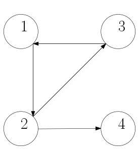
The simulation conditions are as specified in the tables below.

Spacecraft 1 Spacecraft 2 Spacecraft 3 Spacecraft 4
Inertia Matrix 20×𝕀3×320\times\mathbb{I}_{3\times 3} 30×𝕀3×330\times\mathbb{I}_{3\times 3} 40×𝕀3×340\times\mathbb{I}_{3\times 3} 50×𝕀3×350\times\mathbb{I}_{3\times 3}
Initial attitude (MRP) [0.80.80.8]\begin{bmatrix}0.8\\ 0.8\\ 0.8\end{bmatrix} [0.40.40.4]\begin{bmatrix}0.4\\ 0.4\\ 0.4\end{bmatrix} [0.60.60.6]\begin{bmatrix}-0.6\\ -0.6\\ -0.6\end{bmatrix} [0.80.80.8]\begin{bmatrix}-0.8\\ -0.8\\ -0.8\end{bmatrix}
Initial Angular Velocity [0.068490.068490.06849]\begin{bmatrix}0.06849\\ 0.06849\\ 0.06849\end{bmatrix} [000]\begin{bmatrix}0\\ 0\\ 0\end{bmatrix} [0.096150.096150.09615]\begin{bmatrix}-0.09615\\ -0.09615\\ -0.09615\end{bmatrix} [0.068490.068490.06849]\begin{bmatrix}0.06849\\ 0.06849\\ 0.06849\end{bmatrix}
Table 1: Spacecraft Initial conditions and Parameters
121\rightarrow 2 232\rightarrow 3 313\rightarrow 1 242\rightarrow 4
Bound on delay (h) 55 seconds 66 seconds 77 seconds 55 seconds
Bound on delay derivative (d) 11 22 0.50.5 11
Table 2: Time Delay Parameters

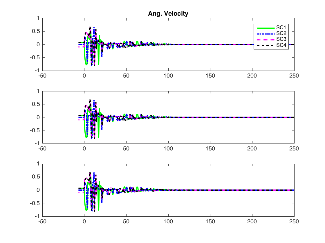
For the given communication topology, lemma  5 yields γ>1.414\gamma>1.414. Thus, the damping gain γ\gamma is set to 55. Theorem  2 yields a conservative upper bound on the delay at 9.6346 seconds. The simulation results are presented below. All vectors are expressed in body frames of the respective spacecraft.

Refer to caption
Figure 4: Spacecraft Attitudes vs Time
Refer to caption
Figure 5: Spacecraft Attitude Derivatives vs Time

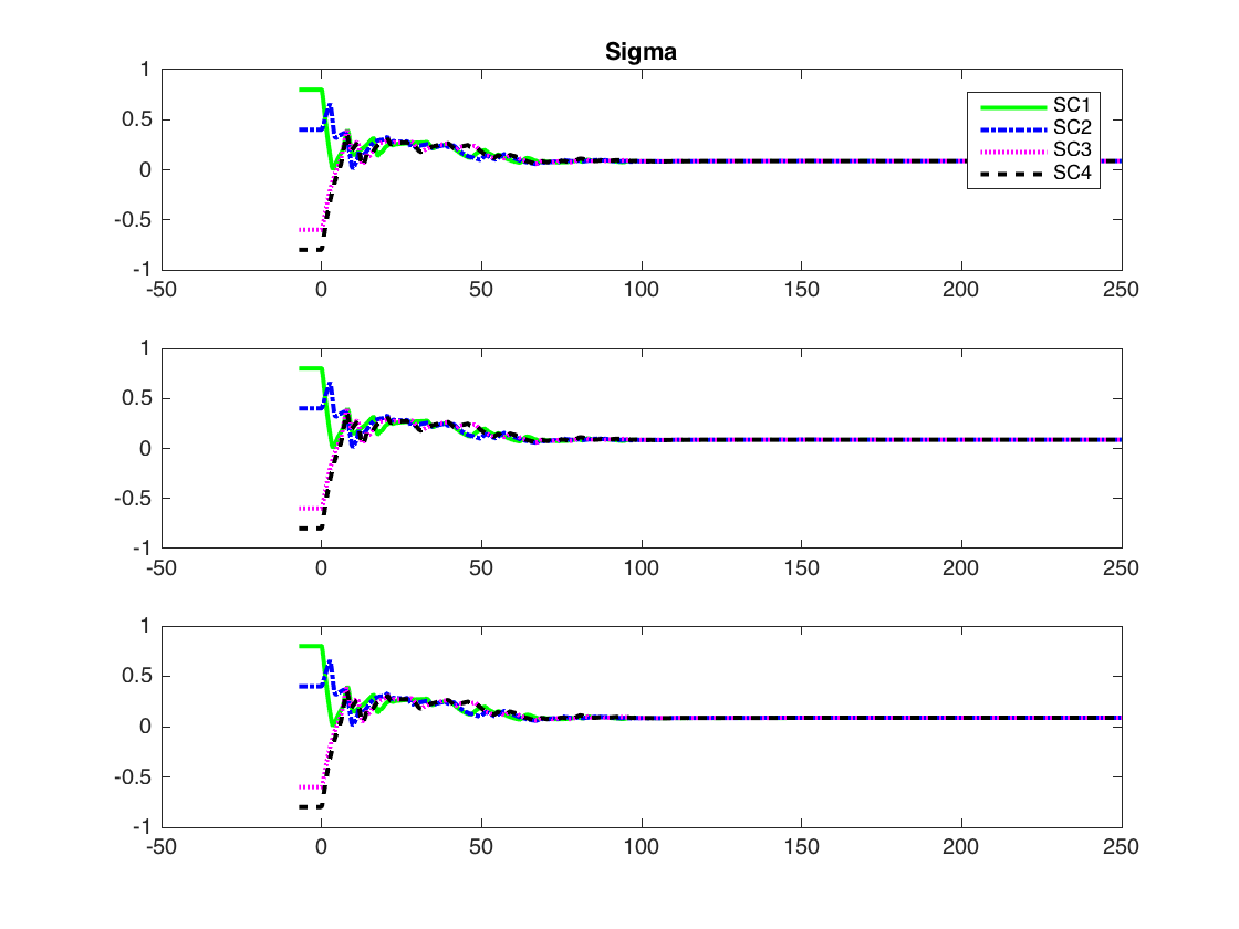
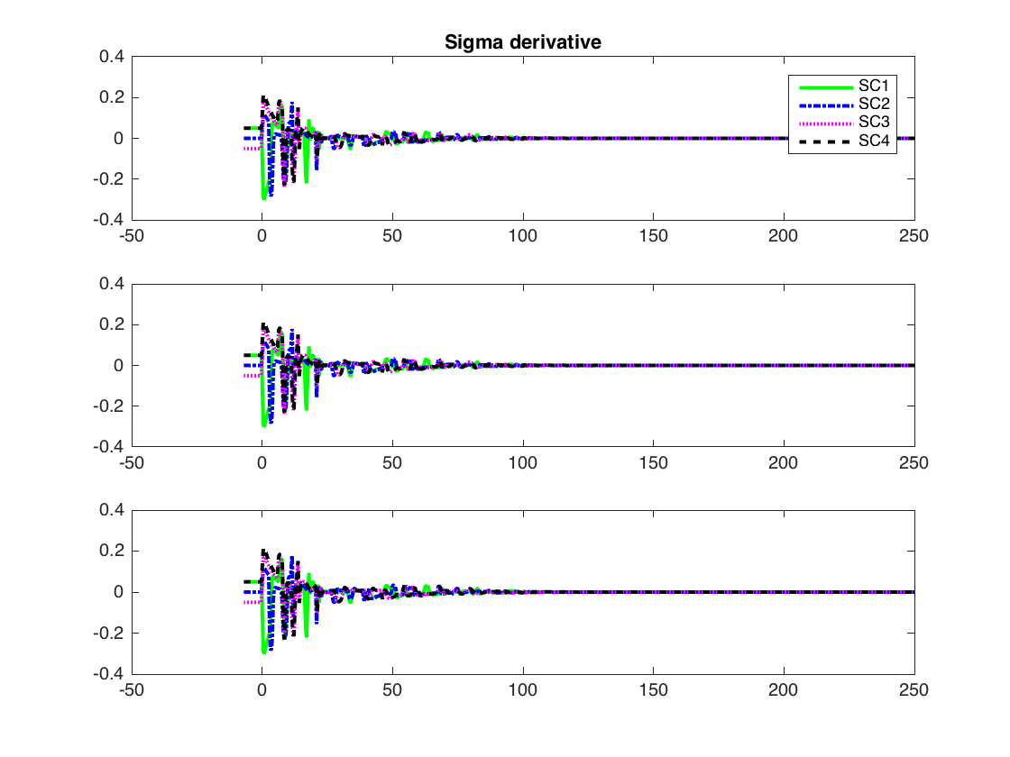
As we can see, the spacecraft achieve consensus.

Refer to caption
Figure 6: Spacecraft Angular Velocities vs Time
Refer to caption
Figure 7: Spacecraft Control Torques vs Time

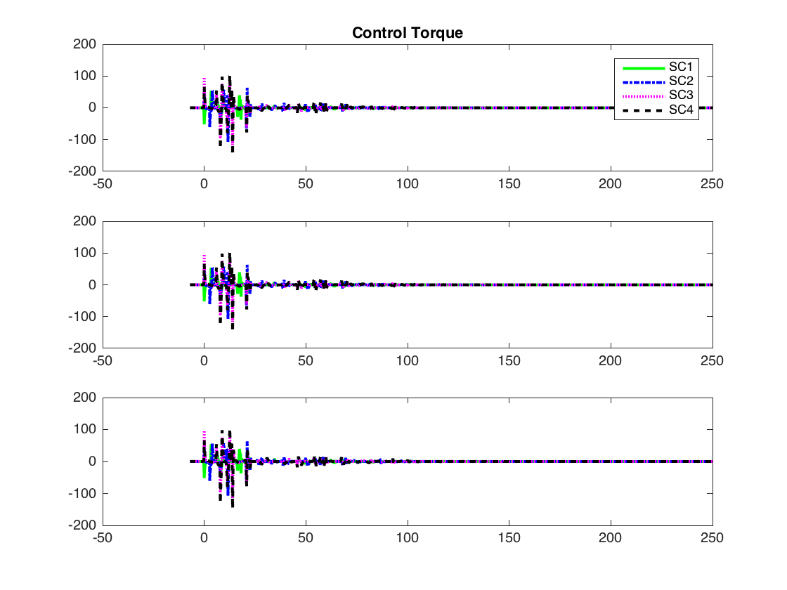
The control torques are obtained by transforming the control input (8) from the [𝝈𝝈˙]\left[{\bm{\sigma}}~\dot{\bm{\sigma}}\right] space back to the [𝝈𝝎]\left[{\bm{\sigma}}~{\bm{\omega}}\right] space. These are the actual torques that are implemented by the respective spacecraft towards achieving the desired consensus.
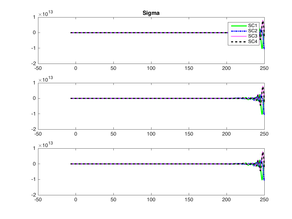
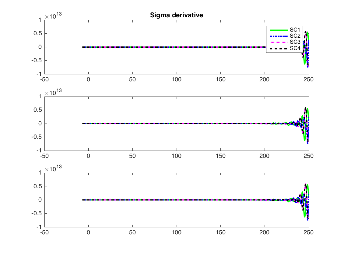
On setting the gain γ\gamma to 0.1, we observe that consensus is not achieved and the states of the spacecraft diverge from each other. The results are shown below.

Refer to caption
Figure 8: Spacecraft Attitudes vs Time when gain γ\gamma is set to 0.1
Refer to caption
Figure 9: Spacecraft Attitude Derivatives vs Time when gain γ\gamma is set to 0.1

5 Summary and Conclusions

Distributed variable time-delays were considered in attitude consensus of multiple cooperating spacecraft. The mathematical proof for consensus was shown using the small-gain theorem for spacecraft formations with a rooted directed spanning tree. Simulation results for a 4 spacecraft attitude consensus scenario were presented.

References

  • [1] R. Olfati-Saber and R. M. Murray, “Consensus problems in networks of agents with switching topology and time-delays,” IEEE Transactions on automatic control, Vol. 49, No. 9, 2004, pp. 1520–1533.
  • [2] R. B. Wei Ren and E. Atkins, “Information consensus in multivehicle cooperative control,” IEEE Control systems magazine, Vol. 27, No. 2, 2007, pp. 71–82.
  • [3] F. H. P. Wang and K. Lau, “Synchronized Formation Rotation and Attitude Control of Multiple Free-flying Spacecraft,” Journal of Guidance, Control and Dynmics, Vol. 22, 1999, pp. 28–35.
  • [4] M. VanDyke and C. Hall, “Decentralized Coordinated Attitude Control within a Formation of Spacecraft,” Journal of Guidance, Control and Dynmics, Vol. 29, No. 5, 2006, pp. 1101–1109.
  • [5] M. Mesbahi and F. Y. Hadaegh, “Formation Flying Control of Multiple Spacecraft via Graphs, Matrix Inequalities, and Switching,” Kohala Coast, Hawai’i, Proceedings of the 1999 IEEE International Conference on Control Applications, 1999.
  • [6] W. Ren, “Distributed attitude alignment in spacecraft formation flying,” International journal of adaptive control and signal processing, Vol. 21, No. 2-3, 2007, pp. 95–113.
  • [7] A. S. M. J. Lin and B. Anderson, “The multi-agent rendezvous problem. Part 1: The synchronous case,” Siam Journal on Control and Optimization, Vol. 46, 2007, pp. 2096–2119.
  • [8] S.-J. Chung, U. Ahsun, and J.-J. E. Slotine, “Application of synchronization to formation flying spacecraft: Lagrangian approach,” Journal of Guidance, Control, and Dynamics, Vol. 32, No. 2, 2009, pp. 512–526.
  • [9] L. Guiming and L. Liangdong, “Coordinated Multiple Spacecraft Attitude Control with Communication Time Delays and Uncertainities,” Chinese Journal of Astronautics, Vol. 25, 2012, p. 698–708.
  • [10] H. D. Shihua Li and P. Shi, “Distributed Attitude Control for Multiple Spacecraft With Communication Delays,” IEEE Transactions on Aerospace and Electronic Systems, Vol. 50, No. 3, 2014, pp. 1765–1773.
  • [11] M. Nazari, E. A. Butcher, T. Yucelen, and A. K. Sanyal, “Decentralized Consensus Control of a Rigid-Body Spacecraft Formation with Communication Delay,” Journal of Guidance, Control, and Dynamics, Vol. 39, No. 4, 2016, pp. 838–851.
  • [12] M. G. Zhou Jiakang and H. Qinglei, “Delay Depending Decentralized Adaptive Attitude Synchronization Tracking Control of Spacecraft Formation,” Chinese Journal of Astronautics, Vol. 25, 2012, p. 406–415.
  • [13] W. Ren and E. Atkins, “Distributed multi-vehicle coordinated control via local information exchange,” International Journal of Robust and Nonlinear Control, Vol. 17, No. 10-11, 2007, pp. 1002–1033.
  • [14] K. G. V. Kharitonov and J. Chen, Stability of time-delay systems. Birkhauser, 2003.
  • [15] C.-Y. Kao and A. Rantzer, “Stability analysis of systems with uncertain time-varying delays,” Automatica, Vol. 43, No. 6, 2007, pp. 959–970.
  • [16] W. Yang, A. L. Bertozzi, and X. Wang, “Stability of a second order consensus algorithm with time delay,” 47th IEEE Conference on Decision and Control, 2008, pp. 2926–2931.