AutoLTS: Automating Cycling Stress Assessment via Contrastive Learning and Spatial Post-processing
Abstract
Cycling stress assessment, which quantifies cyclists’ perceived stress imposed by the built environment and motor traffics, increasingly informs cycling infrastructure planning and cycling route recommendation. However, currently calculating cycling stress is slow and data-intensive, which hinders its broader application. In this paper, We propose a deep learning framework to support accurate, fast, and large-scale cycling stress assessments for urban road networks based on street-view images. Our framework features i) a contrastive learning approach that leverages the ordinal relationship among cycling stress labels, and ii) a post-processing technique that enforces spatial smoothness into our predictions. On a dataset of 39,153 road segments collected in Toronto, Canada, our results demonstrate the effectiveness of our deep learning framework and the value of using image data for cycling stress assessment in the absence of high-quality road geometry and motor traffic data.
1 Introduction
Safety and comfort concerns have been repeatedly identified as major factors that inhibit cycling uptake in cities around the world. A range of metrics, such as the level of traffic stress (LTS) (Furth, Mekuria, and Nixon 2016; Huertas et al. 2020) and bicycle level of service index (Callister and Lowry 2013), have been proposed to quantify cyclists’ perceived stress imposed by the built environment and motor traffic. These metrics are predictive of cycling behaviors (Imani, Miller, and Saxe 2019; Wang et al. 2020) and accidents (Chen et al. 2017), and thus have been applied to support cycling infrastructure planning (Lowry, Furth, and Hadden-Loh 2016; Gehrke et al. 2020; Chan, Lin, and Saxe 2022) and route recommendation (Chen et al. 2017; Castells-Graells, Salahub, and Pournaras 2020). However, calculating these metrics typically requires high-resolution road network data, such as motor traffic speed, the locations of on-street parking, and the presence/type of cycling infrastructure on each road segment. The practical challenge of collecting accurate and up-to-date data hinders the broader application of cycling stress assessment and tools built on it.
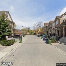
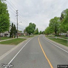
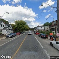
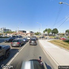
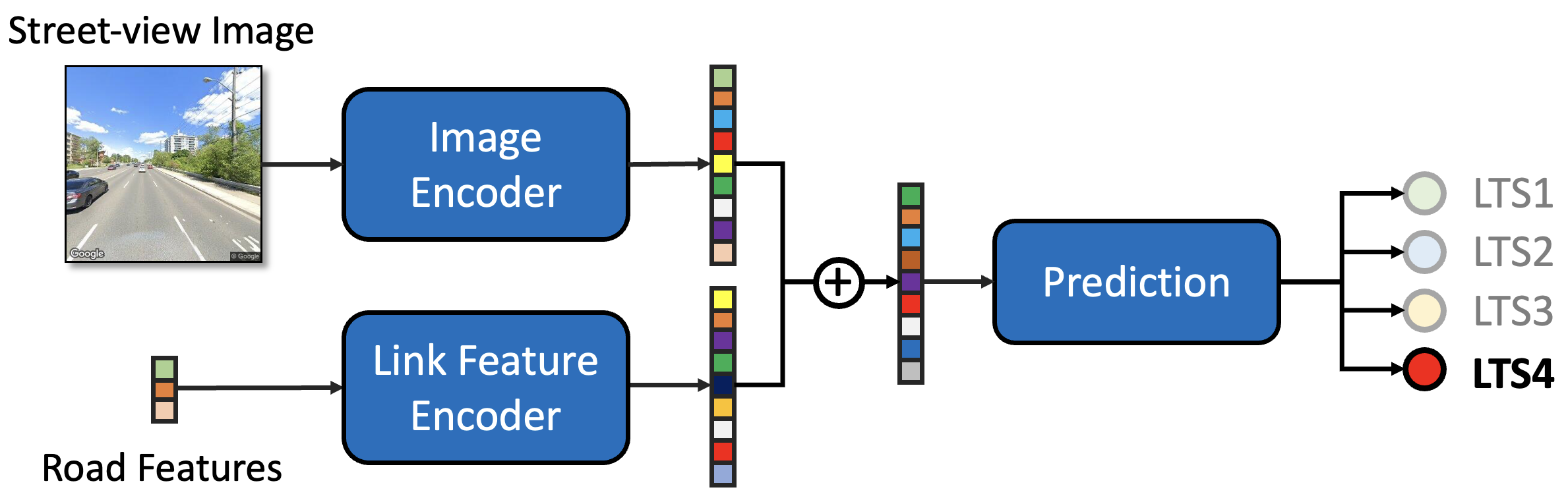
To tackle this challenge, we propose AutoLTS, a deep learning framework for assessing cycling stress of urban road networks based on street-view images. AutoLTS can facilitate timely, accurate, and large-scale assessments of cycling stress because up-to-date street-view images are easy to access via the Google StreetView API. Using a dataset of 39,153 road segments collected in Toronto, Canada, we focus on automating the calculation of the LTS metric. Specifically, as shown in Figure 1, road segments are classified into four classes, i.e., LTS 1, 2, 3 and 4 (Dill and McNeil 2016), corresponding to the cycling suitability of four types of cyclists, where LTS 1 is the least stressful road and LTS 4 is the most stressful. This metric has been applied to investigate the connectivity (Lowry, Furth, and Hadden-Loh 2016; Kent and Karner 2019) and equity (Tucker and Manaugh 2018) of urban cycling networks and to evaluate cycling interventions during the COVID-19 pandemic (Lin, Chan, and Saxe 2021). While we focus on LTS for demonstration, our approach applies to any cycling stress metric.
Formulating this task as a simple image classification problem may not utilize the training dataset to its full potential because it ignores i) the causal relationship between road features and LTS, ii) the ordinal relationships among LTS labels, and iii) the spatial structure of urban road networks. It is critical to leverage i)–iii) to improve the prediction performance as our dataset, limited by the practical data collection challenge and the number of road segments in a city, is relatively small for a computer vision task. Item ii) is of particular importance as misclassifications between different pairs of LTS labels carry different empirical meanings. For example, predicting an LTS1 road as LTS3 is considered worse than predicting it as LTS2 because LTS2 corresponds to the cycling stress tolerance of most adults (Furth, Mekuria, and Nixon 2016). The former may lead to redundant cycling infrastructure on a low-stress road and or recommended cycling routes that exceed most adults’ stress tolerance.
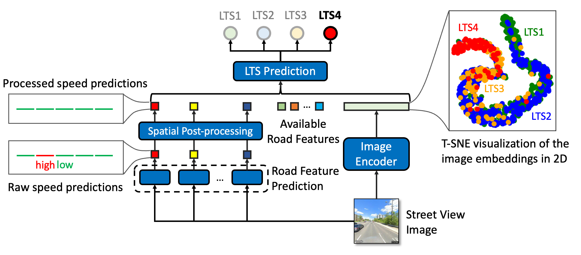
As illustrated in Figure 2, to capture i), we formulate the LTS assessment as a two-step learning task. We first predict LTS related road features based on the input image and learn high-quality representations of the image. We then combine the image embedding with the predicted and available road features to produce the final LTS prediction. This two-step framework allows us to capture ii) and iii) via contrastive learning and a spatial post-processing technique, respectively. Specifically, to address ii), we propose a contrastive learning approach to learn an image embedding space where images are clustered based on their LTS labels, and where these clusters are positioned according to the ordinal relationship among these labels. To tackle iii), we develop a post-processing technique to enforce spatial smoothness into road feature predictions. We opt not to directly enforce spatial smoothness into LTS predictions because it may smooth over important local patterns, which are critical for downstream applications such as cycling network design that aims to fix the disconnections between low-stress sub-networks. Our contributions are summarized below.
-
1.
A novel application. We introduce the first dataset and the first computer vision framework for automating cycling stress assessment.
-
2.
New methodologies. We propose a new contrastive loss for ordinal classification that generalizes the supervised contrastive loss (Khosla et al. 2020). We develop a post-processing technique that adjusts the road feature predictions considering the spatial structure of the road network. Both can be easily generalized to other tasks.
-
3.
Strong performance. Through comprehensive experiments using a dataset collected in Toronto, Canada, we demonstrate i) the value of street-view images for cycling stress assessment, and ii) the effectiveness of our approach in a wide range of real-world settings.
2 Literature Review
Computer vision for predicting urban perceptions.
Street view images have been used to assess the perceived safety, wealth, and uniqueness of neighborhoods (Salesses, Schechtner, and Hidalgo 2013; Arietta et al. 2014; Naik et al. 2014; Ordonez and Berg 2014; Dubey et al. 2016) and to predict neighborhood attributes such as crime rate, housing price, and voting preferences (Arietta et al. 2014; Gebru et al. 2017). We contribute to this stream of literature by i) proposing the first dataset and the deep-learning framework for assessing cycling stress, and ii) developing the first post-processing technique to enforce spatial smoothness in model predictions. Our proposal of automating cycling stress assessment via a computer vision approach is similar to the work of (Ito and Biljecki 2021) who use pre-trained image segmentation and object detection models to extract road features and then construct a bike-ability index based on them. In contrast, we focus on automating the calculation of a cycling stress metric that is well-validated in the transportation literature. The approach proposed by (Ito and Biljecki 2021) does not apply because many LTS-related road features are i) unlabeled in the dataset on which the segmentation and object detection models were trained (e.g. road and cycling infrastructure types) or ii) not observable in street-view images (e.g. motor traffic speed).
Contrastive learning.
Contrastive learning, which learns data representations by contrasting similar and dissimilar data samples, has received growing attention in computer vision. Such techniques usually leverage a contrastive loss to guide the data encoder to pull together similar samples in an embedding space, which has been shown to facilitate downstream learning in many applications (Zhao et al. 2021; Bengar et al. 2021; Bjorck et al. 2021), especially when data labels are unavailable or scarce. To date, most contrastive learning approaches are designed in unsupervised settings (Gutmann and Hyvärinen 2010; Sohn 2016; Oord, Li, and Vinyals 2018; Hjelm et al. 2018; Wu et al. 2018; Bachman, Hjelm, and Buchwalter 2019; He et al. 2020; Chen et al. 2020). They typically generate “similar” data by applying random augmentations to unlabeled data samples. More recently, Khosla et al. (2020) apply contrastive learning in a supervised setting where they define “similar” data as data samples that share the same image label. Linear classifiers trained on the learned embeddings outperform image classifiers trained directly based on images. We extend the supervised contrastive loss (Khosla et al. 2020) by augmenting it with terms that measure the similarity of images with “neighboring” labels. Consequently, the relative positions of the learned embeddings reflect the similarity between their class labels, which helps to improve our model performance.
3 Method
3.1 Data Collection and Pre-processing
Training and testing our model requires three datasets: i) road network topology, ii) ground-truth LTS labels for all road segments, and iii) street-view images that clearly present the road segments. We collect all the data in Toronto, Canada via a collaboration with the City of Toronto. Data sources and pre-processing steps are summarized below.
Road network topology: We retrieve the centerline road network from City of Toronto (2020). Geospatial coordinates of both ends of each road segment are presented. We exclude roads where cycling is legally prohibited, e.g., expressways. The final network has 59,554 road segments.
LTS label. The LTS calculation requires detailed road network data. For each road segment in Toronto, we collect road features as summarized in Table 1 and calculate its LTS label following Furth, Mekuria, and Nixon (2016) and Imani, Miller, and Saxe (2019) (detailed in Appendix B).
Street-view image. We collect street-view images using the Google StreetView API. We opt not to collect images for road segments that are shorter than 50 meters because a significant portion of those images typically present adjacent road segments that may have different LTS labels. For each of the remaining road segments, we collect one image using the geospatial coordinate of its mid-point. We manually examine the collected images to ensure that they clearly present the associated road segments. If an image fails the human screening, we manually recollect the image when possible. Images are missing for roads where driving is prohibited, such as trails and narrow local passageways.
| Feature | Source |
|---|---|
| Road type | (City of Toronto 2020) |
| Road direction | (City of Toronto 2020) |
| Number of lanes | (Government of Canada 2020) |
| Motor traffic speed | (Travel Modelling Group 2016) |
| Cycling infrastructure location | (City of Toronto 2020) |
| On-street parking location | (Toronto Parking Authority 2020) |
Our final image dataset consists of 39,153 high-quality street-view images, with 49.0%, 34.5%, 6.9%, and 9.7% of them labeled as LTS 1, 2, 3 and 4, respectively.
3.2 Supervised Contrastive Learning for Ordinal Classification
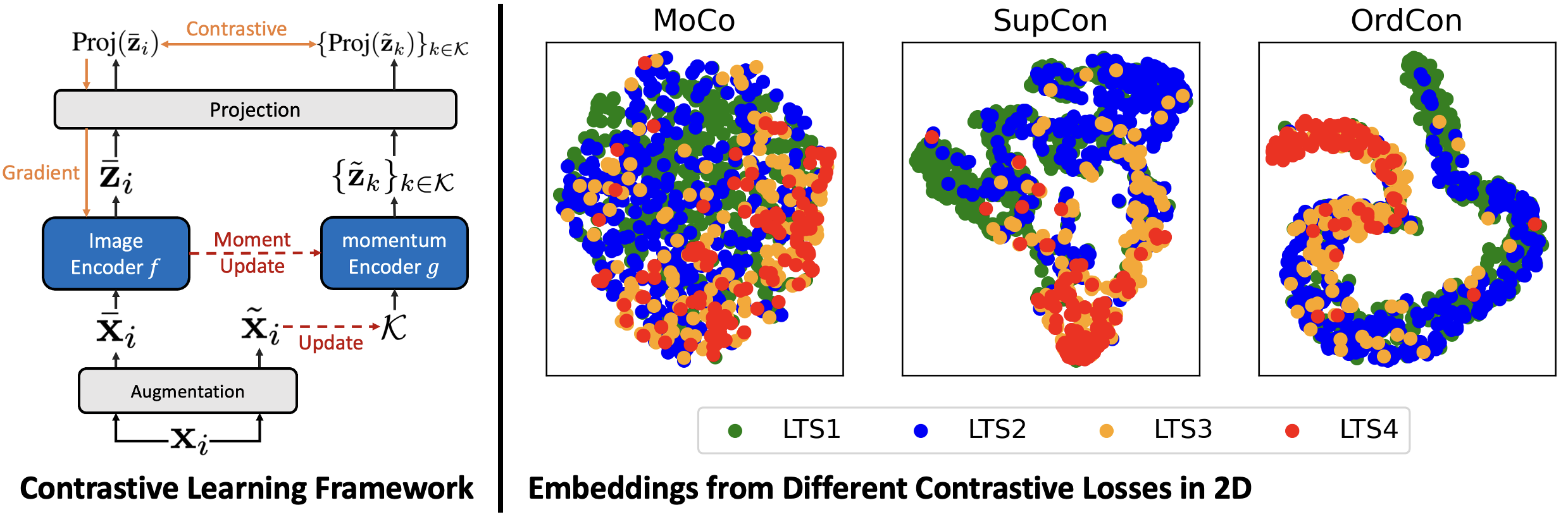
We propose a contrastive learning approach to train the image encoder. The novelty lies in the development of a new contrastive loss that considers the ordinal relationship among LTS labels. We adopt a contrastive learning framework (Figure 3) similar to MoCo (He et al. 2020) to train the image encoder on a pretext task where the encoder learns to pull together “similar” images in the embedding space. Given a batch of road segments indexed by , let and denote the street view image and the label of segment , respectively. We assume are discrete and ordered for all . We create virtual labels for each image where for all . In words, these virtual labels are created by grouping the “neighboring” real labels at different granularities. Consequently, images with “similar” real labels have more overlapping virtual labels. We create two views and of each image by applying a random augmentation module twice. We create a momentum encoder that has the same structure as and whose parameters are updated using the momentum update function (He et al. 2020) as we train . The image views and are encoded by and , respectively, where is a fixed-length queue that stores previously generated image views. Let and denote the embedding generated by these two encoders. During training, these embeddings are further fed into a projection layer, which is discarded during inference following Khosla et al. (2020) and Chen et al. (2020). The encoder network is trained to minimize the following loss that applies to the projected embeddings:
| (1) |
where for all , is a constant weight assigned to the virtual label, is a temperature hyper-parameter, and p is the projection function.
Comparison to other loss functions. Compared to MoCo (He et al. 2020), our OrdCon takes advantage of label information. Consequently, as illustrated in Figure 3, our image embeddings form clusters that correspond to their image labels. Compared to the SupCon (Khosla et al. 2020), our OrdCon considers the ordinal relationship among image labels by aggregating the real label at different granularities. As a result, the relative positions of our embedding clusters reflect the similarity between their corresponding labels. OrdCon recovers the SupCon when and .
3.3 Spatial Post-processing for Road Feature Predictions
Several LTS-related road features, e.g., motor traffic speed, have strong spatial correlations, meaning that the values associated with adjacent road segments are highly correlated. Such structure can be useful in regulating road feature predictions, which may lead to improved LTS predictions. However, it is often not obvious how spatial smoothness should be enforced. For example, consider a case where the motor traffic speeds of five consecutive road segments are predicted as 60, 40, 60, 40, and 60 km/h, respectively. It is likely that two of them are wrong, yet it is unclear if we should change the 40s to 60 or 60s to 40. In this section, we propose a principled way to address this problem.
A Causal Model
We start by introducing a directed arc graph (DAG) (illustrated in Figure 4) that describes the relationships between the inputs (i.e., street view images) and targets (i.e., the road feature of interest) of our road-feature prediction module (illustrated in Figure 2). We assume to be discrete. This is not restrictive because continuous road features can be categorized according to the LTS calculation scheme (detailed in Appendix C). Let denote the set of edges in the road network and denote the set of road segments that are adjacent to road segment . We make three assumptions as listed below.
-
1.
For any and , and are conditionally independent given .
-
2.
For any and , and are conditionally independent given .
-
3.
For any and and , and are conditionally independent given .
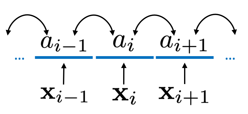
The first and second assumptions state that the target is directly influenced only by the input of the same road segment and the targets of its adjacent segments . The third assumption states that when target is known, its impacts on its adjacent targets are independent. This model naturally applies to several LTS-related road features. For example, the traffic speed on a road segment is affected by the built environment observable from its street-view image () and the traffic speeds on its adjacent road segments (). The built environment and traffic speeds on other road segments may present indirect impacts on the road segment of interest, but such impacts must transmit through its adjacent road segments. Additionally, the impacts of the traffic speed on a road segment on the speeds of its adjacent road segments can be viewed as independent (or weakly dependent) because they usually correspond to motor traffics along different directions.
Enforcing Spatial Smoothness
Given the DAG, target predictions can be jointly determined by maximizing the joint probability of all targets given all inputs, i.e., . However, evaluating the joint distribution of is non-trivial because our DAG is cyclic. Instead, we look into determining the target of one road segment at a time assuming all other targets are fixed.
Proposition 1.
Under assumptions 1–3, for any ,
| (2) |
Proposition 2 decomposes the conditional probability of target given all other targets and inputs. The transition probability can be estimated from our training data, and can be produced by our deep learning model. The proof is presented in Appendix A. Inspired by Proposition 2, we next introduce an algorithm that iteratively updates the target predictions in the whole network until there are no further changes. The algorithm is summarized in Algorithm 1.
Input: Initial predictions ; Transition Probabilities ; Model Predictions ; Adjacent sets for any .
Output: Updated predictions .
4 Empirical Results
4.1 Experiment Setup
Evaluation scenarios. We evaluate AutoLTS and baseline methods in three data-availability scenarios, each under four train-test-validation splits, totaling 12 sets of experiments.
For data availability, we consider LTS based on
-
1.
Street view image
-
2.
Street view image, road and cycling infrastructure types
-
3.
Street view image, number of lanes, and speed limit.
The design of these scenarios is informed by the real data collection challenges we encountered in Toronto. The number of lanes and the speed limit of each road segment are accessed via Open Data Canada (Government of Canada 2020). Road type and the location of cycling infrastructure are available via Open Data Toronto (City of Toronto 2020). However, as the two data platforms use different base maps, combining data from these two sources requires considerable manual effort, echoing the data collection challenges in many other cities.
For the train-test-validation split, we consider
-
1.
A random 70/15/15 train-test-validation split across all road segments in Toronto.
-
2.
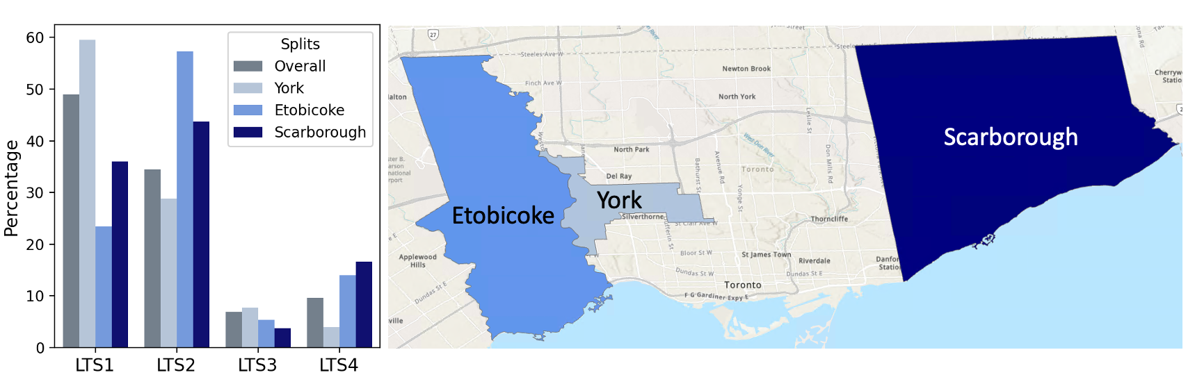
Three spatial splits, which use road segments in an area as the test set and performs a random 80/20 train-validation split for other road segments. As shown in Figure 5, we consider using road segments in three of Toronto’s amalgamated cities, York, Etobicoke, and Scarborough as the test sets. These three areas have very different LTS distributions, which allows us to exam the generalization ability of AutoLTS in real-world settings.
The random split mimics the situation where we use AutoLTS to extrapolate manual LTS assessment or to update the LTS assessment in the city where the model is trained. The spatial split mimics the situation where we apply AutoLTS trained in one city to an unseen city.
Evaluation Metrics.
-
•
LTS Prediction Accuracy
(3) -
•
High/Low-Stress Prediction Accuracy
(4) where is a function that takes a value of if the input LTS label is low-stress (LTS1/2) and takes if the LTS label is high-stress (LTS3/4).
-
•
Average False High/Low-Stress Rate
(5) where and denote, respectively, the numbers of test road segments that are low- and high-stress.
Acc and HLA measure the overall prediction performance, while AFR considers the fact that the dataset is imbalanced with a higher portion being low-stress. Ideally, we want a model that achieves high Acc and HLA and low AFR.
|
|
|
|
||||||||||||||||||
| Sce. | Method | Acc | HLA | AFR | Acc | HLA | AFR | Acc | HLA | AFR | Acc | HLA | AFR | ||||||||
| 1 | Cross-Entropy | 70.49 | 93.51 | 10.19 | 60.97 | 93.40 | 12.09 | 64.20 | 92.89 | 9.37 | 64.28 | 93.87 | 12.61 | ||||||||
| MoCo | 61.69 | 90.23 | 14.68 | 57.68 | 91.34 | 17.17 | 52.03 | 89.89 | 12.71 | 56.16 | 91.45 | 17.01 | |||||||||
| SupCon | 70.75 | 93.41 | 11.73 | 61.17 | 93.40 | 17.05 | 64.29 | 93.19 | 9.29 | 65.73 | 93.38 | 10.96 | |||||||||
| AutoLTS | 73.41 | 94.16 | 10.50 | 62.31 | 94.69 | 15.72 | 64.69 | 93.50 | 9.87 | 66.04 | 94.62 | 10.77 | |||||||||
| 2 | CART | 56.21 | 96.87 | 5.21 | 43.33 | 96.75 | 4.51 | 35.35 | 96.73 | 7.25 | 50.22 | 96.40 | 8.34 | ||||||||
| Cross-Entropy | 75.07 | 96.82 | 5.91 | 63.37 | 96.37 | 5.26 | 66.21 | 95.97 | 6.55 | 67.76 | 95.74 | 10.14 | |||||||||
| MoCo | 68.94 | 96.65 | 14.41 | 57.39 | 96.22 | 4.81 | 59.11 | 95.79 | 9.08 | 62.09 | 96.31 | 8.66 | |||||||||
| SupCon | 74.89 | 96.42 | 6.33 | 64.13 | 96.17 | 5.54 | 65.70 | 95.68 | 9.14 | 68.55 | 96.19 | 8.66 | |||||||||
| AutoLTS | 75.86 | 96.22 | 7.02 | 65.04 | 96.13 | 8.77 | 67.74 | 96.20 | 7.37 | 68.86 | 96.51 | 7.78 | |||||||||
| 3 | CART | 89.41 | 96.07 | 10.08 | 88.81 | 97.57 | 6.97 | 90.67 | 95.46 | 10.37 | 91.90 | 94.90 | 12.51 | ||||||||
| Cross-Entropy | 90.26 | 95.33 | 8.97 | 88.12 | 97.37 | 6.47 | 91.01 | 95.34 | 7.79 | 91.45 | 95.54 | 12.88 | |||||||||
| MoCo | 89.82 | 95.37 | 11.25 | 86.90 | 98.61 | 3.63 | 90.88 | 96.35 | 6.78 | 92.74 | 94.91 | 12.79 | |||||||||
| SupCon | 91.20 | 96.19 | 11.30 | 87.42 | 96.70 | 4.18 | 89.04 | 95.93 | 7.69 | 92.41 | 95.11 | 11.50 | |||||||||
| AutoLTS | 91.65 | 96.70 | 5.87 | 89.24 | 97.23 | 4.78 | 92.61 | 96.68 | 4.77 | 94.50 | 97.28 | 5.81 | |||||||||
Baselines. To demonstrate the value of image data, in scenarios where road features are available, we use a classification and regression tree (CART) that predicts LTS based on available road features as a baseline. CART is selected because the LTS calculation scheme (Furth, Mekuria, and Nixon 2016) can be summarized by a decision tree. We also compare AutoLTS with image-based supervised and contrastive learning methods. For supervised learning, we consider Res-50 (He et al. 2016) trained using the cross-entropy loss. For contrastive learning, we consider supervised contrastive learning (MoCo) (He et al. 2020) and self-supervised contrastive learning (SupCon) (Khosla et al. 2020), both implemented with the MoCo trick (He et al. 2020). Baselines are detailed in Appendix E.
Model details. We use ResNet-50 (He et al. 2016) as the image encoder. The normalized ReLU activations of the final pooling layer are used as the image embedding (=2,048). We follow He et al. (2020) to set and use the SimCLR augmentation (Chen et al. 2020) for training. We train one ResNet-50 to predict each missing road feature. All road features are discretized using the thresholds defined in the LTS calculation scheme (Furth, Mekuria, and Nixon 2016) (Appendix C). In the LTS prediction module, we first train a CART model to predict a road segment’s LTS based on its predicted and available road features. We then use the LTS distribution in the leaf node that a road segment is assigned to as its road feature embedding, which is mapped to a -dimensional space via a linear layer and averaged with the image embedding. Finally, a linear classifier predicts the road segment’s LTS based on the averaged embedding. Training details are summarized in Appendix D.
|
|
|
|
|||||||||||||||||
| Model | Acc | HLA | AFR | Acc | HLA | AFR | Acc | HLA | AFR | Acc | HLA | AFR | ||||||||
| 2Step-Exact | 41.97 | 52.41 | 33.89 | 57.05 | 84.41 | 29.92 | 23.23 | 42.31 | 39.09 | 24.18 | 35.90 | 45.31 | ||||||||
| 2Step-Spatial-Exact | 43.10 | 54.20 | 32.28 | 58.06 | 85.41 | 21.60 | 23.46 | 44.10 | 38.81 | 25.39 | 37.79 | 43.12 | ||||||||
| MoCo-NN | 61.69 | 90.23 | 14.68 | 57.68 | 91.34 | 17.17 | 52.03 | 89.89 | 12.71 | 56.16 | 91.45 | 17.01 | ||||||||
| SupCon-NN | 70.75 | 93.41 | 11.73 | 61.17 | 93.40 | 17.05 | 64.29 | 93.59 | 9.45 | 65.73 | 93.38 | 10.96 | ||||||||
| OrdCon-NN | 71.11 | 93.96 | 9.95 | 60.74 | 93.93 | 11.62 | 64.02 | 93.98 | 9.29 | 65.95 | 94.54 | 10.55 | ||||||||
| AutoLTS-MoCo | 72.21 | 93.70 | 10.11 | 61.60 | 94.02 | 13.52 | 64.69 | 92.94 | 9.84 | 64.40 | 94.05 | 11.62 | ||||||||
| AutoLTS-SupCon | 73.30 | 94.16 | 10.61 | 62.17 | 94.38 | 15.76 | 64.63 | 93.42 | 10.66 | 65.86 | 94.37 | 11.43 | ||||||||
| AutoLTS-OrdCon | 73.41 | 94.16 | 10.50 | 62.31 | 94.69 | 15.72 | 64.69 | 93.50 | 9.87 | 66.04 | 94.62 | 10.77 | ||||||||
4.2 Main Results
The performance of AutoLTS and baselines are shown in Table 2. We summarize our findings below.
The value of image data for cycling stress assessment. AutoLTS achieves LTS prediction accuracy of 62.31%–73.41% and high/low-stress accuracy of 93.50%–94.69% only using street-view images. Such a model can be useful for cycling infrastructure planning and route recommendation tools that do not require the granularity of four LTS categories and focus solely on the difference between high- (LTS3/4) and low-stress (LTS1/2) road segments. In data-availability scenarios where partial road features are available (scenarios two and three), incorporating street-view images leads to increases of 0.43–32.39 percentage points in Acc with little to no increases in AFR. The improvements are particularly large in scenario two where the average increase in Acc due to the usage of street-view images is 23.10 percentage points across all train-test-validation splits considered. By combining street-view images with the speed limit and the number of lanes (scenario 3), the Acc is over 90% under all splits. These numbers demonstrate that street view images are valuable for cycling stress assessment with and without partial road features.
The performance of AutoLTS and other image-based methods. Overall, AutoLTS achieves the highest Acc, which is of primary interest, in all evaluation scenarios. Due to the limited sample size, unsupervised contrastive learning (MoCo) generally falls around 10% behind SupCon. SupCon outperforms the simple image classification formulation (Cross-Entropy) in 8 out of 12 scenarios yet is inferior to AutoLTS in all scenarios. However, we observe that when there is a significant domain shift from training to test data (spatial splits), all methods including AutoLTS are more prone to overfitting the training data, and thus have worse out-of-sample performance than in random splits.
4.3 Ablation Studies
Next, we present ablation studies using data-availability scenario one to demonstrate the values of our two-step learning framework, ordinal contrastive learning loss, and the post-processing module, The results are summarized in Table 3.
The value of the two-step learning framework. We compare AutoLTS with an alternative approach that replaces the LTS prediction module with the exact LTS calculation scheme (2Step-Exact and 2Step-Spatial-Exact). This change leads to reductions of 6.16–40.83 percentage points in Acc due to the compounded errors from the first step, highlighting the importance of second-step learning. Moreover, AutoLTS outperforms all baselines that predict LTS based only on image (MoCo-, SupCon-, and OrdCon-NN), demonstrating the value of incorporating road feature predictions.
The value of ordinal contrastive learning. We compare the three contrastive learning methods using the AutoLTS framework and the linear classification protocol (He et al. 2020). When used to predict LTS without road features (MoCo-, SupCon-, and OrdCon-NN), OrdCon and SupCon are competitive in Acc, yet OrdCon constantly achieves higher HLA and lower AFR because it considers the relationship among LTS labels. This is practically important because the ability to distinguish between low- and high-stress roads plays a vital role in most adults’ cycling decision makings (Furth, Mekuria, and Nixon 2016). When combined with road features, all contrastive learning methods perform reasonably well. Nevertheless, Auto-OrdCon consistently outperforms others by a meaningful margin.
The value of spatial post-processing. Applying the spatial post-processing technique to road feature predictions generally leads to an increase of around 1% in road feature prediction accuracy (presented in Appendix C) which can be translated into improvements in LTS prediction Acc (2Step-Exact versus 2Step-Spatial-Exact). While the improvement seems to be limited, it corresponds to correctly assessing the LTS of 21–162 road segments in the studied area, which can have a significant impact on the routing and cycling infrastructure planning decisions derived based on the assessment.
5 Conclusion
In this paper, we present a deep learning framework, AutoLTS, that uses streetview images to automate cycling stress assessment. AutoLTS features i) a contrastive learning approach that learns image representations that preserve the ordinal relationship among image labels and ii) a post-processing technique that enforces spatial smoothness into the predictions. We show that AutoLTS can assist in accurate, timely, and large-scale cycling stress assessment in the absence of road network data.
Our paper has three limitations, underscoring potential future research directions. First, we observe performance degradation when the training and test data have very different label distributions (spatial splits). Future research may apply domain adaptation methods to boost the performance of AutoLTS in such scenarios. Second, AutoLTS does not consider the specific needs of downstream applications. For instance, in cycling route recommendations, under-estimation of cycling stress may be more harmful than over-estimation because the former may lead to cycling routes that exceed cyclists’ stress tolerance and result in increased risks of cycling accidents. In cycling network design, cycling stress predictions might be more important on major roads than on side streets because cycling infrastructure is typically constructed on major roads. Such impacts may be captured by modifying the loss function to incorporate decision errors. Finally, all our experiments are based on a dataset collected in Toronto. Future research may collect a more comprehensive dataset to further assess the generalizability of our model. We hope this work will open the door to using deep learning to support the broader application of cycling stress assessment and to inform real-world decision makings that improve transportation safety and efficiency.
References
- Arietta et al. (2014) Arietta, S. M.; Efros, A. A.; Ramamoorthi, R.; and Agrawala, M. 2014. City forensics: Using visual elements to predict non-visual city attributes. IEEE Transactions on Visualization and Computer Graphics, 20(12): 2624–2633.
- Bachman, Hjelm, and Buchwalter (2019) Bachman, P.; Hjelm, R. D.; and Buchwalter, W. 2019. Learning representations by maximizing mutual information across views. In Advances in Neural Information Processing Systems.
- Bengar et al. (2021) Bengar, J. Z.; van de Weijer, J.; Twardowski, B.; and Raducanu, B. 2021. Reducing label effort: Self-supervised meets active learning. In Proceedings of the IEEE/CVF International Conference on Computer Vision, 1631–1639.
- Bjorck et al. (2021) Bjorck, J.; Rappazzo, B. H.; Shi, Q.; Brown-Lima, C.; Dean, J.; Fuller, A.; and Gomes, C. P. 2021. Accelerating Ecological Sciences from Above: Spatial Contrastive Learning for Remote Sensing. In Thirty-Fifth AAAI Conference on Artificial Intelligence, AAAI 2021, 14711–14720.
- Callister and Lowry (2013) Callister, D.; and Lowry, M. 2013. Tools and strategies for wide-scale bicycle level-of-service analysis. Journal of Urban Planning and Development, 139(4): 250–257.
- Castells-Graells, Salahub, and Pournaras (2020) Castells-Graells, D.; Salahub, C.; and Pournaras, E. 2020. On cycling risk and discomfort: urban safety mapping and bike route recommendations. Computing, 102(5): 1259–1274.
- Chan, Lin, and Saxe (2022) Chan, T. C. Y.; Lin, B.; and Saxe, S. 2022. A Machine Learning Approach to Solving Large Bilevel and Stochastic Programs: Application to Cycling Network Design. arXiv preprint arXiv:2209.09404.
- Chen et al. (2017) Chen, C.; Anderson, J. C.; Wang, H.; Wang, Y.; Vogt, R.; and Hernandez, S. 2017. How bicycle level of traffic stress correlate with reported cyclist accidents injury severities: A geospatial and mixed logit analysis. Accident Analysis & Prevention, 108: 234–244.
- Chen et al. (2020) Chen, T.; Kornblith, S.; Norouzi, M.; and Hinton, G. 2020. A simple framework for contrastive learning of visual representations. In International Conference on Machine Learning, 1597–1607. PMLR.
- City of Toronto (2020) City of Toronto. 2020. City of Toronto Open Data. https://www.toronto.ca/city-government/data-research-maps/open-data/. Accessed: 2020-09-15.
- Dill and McNeil (2016) Dill, J.; and McNeil, N. 2016. Revisiting the four types of cyclists: Findings from a national survey. Transportation Research Record, 2587(1): 90–99.
- Dubey et al. (2016) Dubey, A.; Naik, N.; Parikh, D.; Raskar, R.; and Hidalgo, C. A. 2016. Deep learning the city: Quantifying urban perception at a global scale. In European Conference on Computer Vision, 196–212. Springer.
- Furth, Mekuria, and Nixon (2016) Furth, P. G.; Mekuria, M. C.; and Nixon, H. 2016. Network connectivity for low-stress bicycling. Transportation Research Record, 2587(1): 41–49.
- Gebru et al. (2017) Gebru, T.; Krause, J.; Wang, Y.; Chen, D.; Deng, J.; Aiden, E. L.; and Fei-Fei, L. 2017. Using deep learning and Google Street View to estimate the demographic makeup of neighborhoods across the United States. Proceedings of the National Academy of Sciences, 114(50): 13108–13113.
- Gehrke et al. (2020) Gehrke, S. R.; Akhavan, A.; Furth, P. G.; Wang, Q.; and Reardon, T. G. 2020. A cycling-focused accessibility tool to support regional bike network connectivity. Transportation Research Part D: Transport and Environment, 85: 102388.
- Government of Canada (2020) Government of Canada. 2020. Government of Canada Open Data. https://open.canada.ca/en/open-data. Accessed: 2020-09-15.
- Gutmann and Hyvärinen (2010) Gutmann, M.; and Hyvärinen, A. 2010. Noise-contrastive estimation: A new estimation principle for unnormalized statistical models. In Proceedings of the Thirteenth International Conference on Artificial Intelligence and Statistics, 297–304. JMLR Workshop and Conference Proceedings.
- He et al. (2020) He, K.; Fan, H.; Wu, Y.; Xie, S.; and Girshick, R. 2020. Momentum contrast for unsupervised visual representation learning. In Proceedings of the IEEE/CVF Conference on Computer Vision and Pattern Recognition, 9729–9738.
- He et al. (2016) He, K.; Zhang, X.; Ren, S.; and Sun, J. 2016. Deep residual learning for image recognition. In Proceedings of the IEEE Conference on Computer Vision and Pattern Recognition, 770–778.
- Hinton and Roweis (2002) Hinton, G. E.; and Roweis, S. 2002. Stochastic neighbor embedding. In Advances in Neural Information Processing Systems, volume 15.
- Hjelm et al. (2018) Hjelm, R. D.; Fedorov, A.; Lavoie-Marchildon, S.; Grewal, K.; Bachman, P.; Trischler, A.; and Bengio, Y. 2018. Learning deep representations by mutual information estimation and maximization. In International Conference on Learning Representations.
- Huertas et al. (2020) Huertas, J. A.; Palacio, A.; Botero, M.; Carvajal, G. A.; van Laake, T.; Higuera-Mendieta, D.; Cabrales, S. A.; Guzman, L. A.; Sarmiento, O. L.; and Medaglia, A. L. 2020. Level of traffic stress-based classification: A clustering approach for Bogotá, Colombia. Transportation Research Part D: Transport and Environment, 85: 102420.
- Imani, Miller, and Saxe (2019) Imani, A. F.; Miller, E. J.; and Saxe, S. 2019. Cycle accessibility and level of traffic stress: A case study of Toronto. Journal of Transport Geography, 80: 102496.
- Ito and Biljecki (2021) Ito, K.; and Biljecki, F. 2021. Assessing bikeability with street view imagery and computer vision. Transportation Research Part C: Emerging Technologies, 132: 103371.
- Kent and Karner (2019) Kent, M.; and Karner, A. 2019. Prioritizing low-stress and equitable bicycle networks using neighborhood-based accessibility measures. International Journal of Sustainable Transportation, 13(2): 100–110.
- Khosla et al. (2020) Khosla, P.; Teterwak, P.; Wang, C.; Sarna, A.; Tian, Y.; Isola, P.; Maschinot, A.; Liu, C.; and Krishnan, D. 2020. Supervised contrastive learning. Advances in Neural Information Processing Systems, 33: 18661–18673.
- Lin, Chan, and Saxe (2021) Lin, B.; Chan, T. C. Y.; and Saxe, S. 2021. The impact of COVID-19 cycling infrastructure on low-stress cycling accessibility: A case study in the City of Toronto. Findings, 19069.
- Lowry, Furth, and Hadden-Loh (2016) Lowry, M. B.; Furth, P.; and Hadden-Loh, T. 2016. Prioritizing new bicycle facilities to improve low-stress network connectivity. Transportation Research Part A: Policy and Practice, 86: 124–140.
- Naik et al. (2014) Naik, N.; Philipoom, J.; Raskar, R.; and Hidalgo, C. 2014. Streetscore-predicting the perceived safety of one million streetscapes. In Proceedings of the IEEE Conference on Computer Vision and Pattern Recognition Workshops, 779–785.
- Oord, Li, and Vinyals (2018) Oord, A. v. d.; Li, Y.; and Vinyals, O. 2018. Representation learning with contrastive predictive coding. arXiv preprint arXiv:1807.03748.
- Ordonez and Berg (2014) Ordonez, V.; and Berg, T. L. 2014. Learning high-level judgments of urban perception. In European Conference on Computer Vision, 494–510. Springer.
- Salesses, Schechtner, and Hidalgo (2013) Salesses, P.; Schechtner, K.; and Hidalgo, C. A. 2013. The collaborative image of the city: mapping the inequality of urban perception. PloS One, 8(7): e68400.
- Sohn (2016) Sohn, K. 2016. Improved Deep metric Learning with Multi-class N-pair Loss Objective. In Advances in Neural Information Processing Systems, volume 29.
- Toronto Parking Authority (2020) Toronto Parking Authority. 2020. Personal Communication. Accessed: 2020-10-26.
- Travel Modelling Group (2016) Travel Modelling Group. 2016. GTAModel V4 Introduction. https://tmg.utoronto.ca/doc/1.6/gtamodel/index.html. Accessed: 2020-11-20.
- Tucker and Manaugh (2018) Tucker, B.; and Manaugh, K. 2018. Bicycle equity in Brazil: Access to safe cycling routes across neighborhoods in Rio de Janeiro and Curitiba. International Journal of Sustainable Transportation, 12(1): 29–38.
- Wang et al. (2020) Wang, K.; Akar, G.; Lee, K.; and Sanders, M. 2020. Commuting patterns and bicycle level of traffic stress (LTS): Insights from spatially aggregated data in Franklin County, Ohio. Journal of Transport Geography, 86: 102751.
- Wu et al. (2018) Wu, Z.; Xiong, Y.; Yu, S. X.; and Lin, D. 2018. Unsupervised feature learning via non-parametric instance discrimination. In Proceedings of the IEEE Conference on Computer Vision and Pattern Recognition, 3733–3742.
- Zhao et al. (2021) Zhao, N.; Wu, Z.; Lau, R. W. H.; and Lin, S. 2021. What Makes Instance Discrimination Good for Transfer Learning? In International Conference on Learning Representations.
Appendix A Proof of Statements
A.1 Proof of Proposition 2
Proof.
We have
The first equation follows the definition of conditional probability. The second equation holds because of the assumptions 1, 2, and 3 presented in Section 3.3. Since the denominator in the last line is a constant, we have
| (6) |
∎
Appendix B LTS Calculation Details
We follow Furth, Mekuria, and Nixon (2016) and Imani, Miller, and Saxe (2019) to calculate the LTS label of every road segment in Toronto. The calculation scheme can be summarized by the following decision rules, which are applied in sequence.
-
•
Road segments that are multi-use pathways, walkway, or trails are LTS 1.
-
•
Road segment with cycle tracks (i.e. protected bike lanes) are LTS 1.
-
•
For road segments with painted bike lanes:
-
–
If the road segment has on-street parking,
-
*
If one lane per direction and motor traffic speed 40 km/h, then LTS 1.
-
*
If one lane per direction and motor traffic speed 48 km/h, then LTS 2.
-
*
If motor traffic speed 56 km/h, then LTS 3.
-
*
Otherwise, LTS4.
-
*
-
–
If the road segment has no on-street parking,
-
*
If one lane per direction and motor traffic speed 48 km/h, then LTS 1.
-
*
If one/two lanes per direction, then LTS 2.
-
*
If motor traffic speed 56 km/h, then LTS 3
-
*
Otherwise, LTS 4.
-
*
-
–
-
•
For road segments without cycling infrastructure:
-
–
If motor traffic speed 40 km/h, and 3 lanes in both directions,
-
*
If daily motor traffc volume 3000, then LTS 1.
-
*
Otherwise, LTS 2.
-
*
-
–
If motor traffic speed 48 km/h, and 3 lanes in both directions,
-
*
If daily motor traffc volume 3000, then LTS 2.
-
*
Otherwise, LTS 3.
-
*
-
–
If motor traffic speed 40 km/h, and 5 lanes in both directions, then LTS 3.
-
–
Otherwise, LTS 4.
-
–
Appendix C Road Feature Prediction Details
C.1 Label Discretization
We discretize all the road features as summarized in Table 4. Threshold values and feature categories are selected following Furth, Mekuria, and Nixon (2016) and Imani, Miller, and Saxe (2019). All road feature prediction problems are then formulated as image classfication problems.
| Road Feature | Label | Definition |
|---|---|---|
| Motor traffic speed | 1 | 40 km/h |
| 2 | 40 – 48 km/h | |
| 3 | 48 – 56 km/h | |
| 4 | km/h | |
| Road type | 1 | Major/minor arterial, arterial ramp |
| 2 | Collector, access road, laneway, local road, others | |
| 3 | Trail, walkway | |
| Number of lanes | 1 | One lane in both directions |
| 2 | Two lanes in both directions | |
| 3 | Three lanes in both directions | |
| 4 | Four lanes in both directions | |
| 5 | More than 5 lanes in both directions | |
| Road direction | 1 | Unidirectional road |
| 2 | Bidirectional road | |
| Cycling infrastructure type | 1 | Bike Lane |
| 2 | Cycle track | |
| 3 | Multi-use pathway | |
| 4 | Others or no cycling infrastructure | |
| On-street parking | 1 | Has on-street parking |
| 2 | No on-street parking |
C.2 Model Details
We train one ResNet-50 (He et al. 2016) to predict each road feature based on the input streetview image. We initialize the model with the weights pre-trained on the ImageNet. We replace the final layer with a fully connected layer whose size corresponds to the number of possible discrete labels for the road feature. We train the model with a standard cross-entropy loss.
C.3 Prediction Performance
We first present the road feature prediction accuracy under the random train-test-validation split (Tabel 5). We compare the performance of Res50 with a naive approach that predicts road features as the corresponding majority classes observed in the training set. We observe that Res50 provides improvements of 1.86%-22.31% for all road features except road direction. This is because the road direction labels are highly imbalanced with over 94% of the road segments being bi-directional. The Res50 model is able to identify some uni-directional road segments at the cost of miss-predicting some bi-directional road segments as uni-directional. We opt to use Res50 despite that it has a lower prediction accuracy than the naive approach because it leads to better prediction performance for AutoLTS according to our experiments.
| Road Feature | Res50 | Naive | Diff. |
|---|---|---|---|
| Road type | 89.97 | 67.66 | +22.31 |
| Motor traffic speed | 71.28 | 54.48 | +16.80 |
| Motor traffic volume | 88.13 | 70.81 | +17.32 |
| Number of lanes | 82.66 | 66.34 | +16.32 |
| Cycling infrastructure | 95.30 | 94.35 | +0.95 |
| On-street parking | 96.05 | 94.19 | +1.86 |
| Road direction | 94.04 | 94.18 | -0.14 |
We next present the road feature prediction results for all train-test-validation splits considered (Table 6). The model performance is similar across different splits, with minor changes in prediction accuracy due to the changes in label distributions.
| Road Feature | Random | York | Etobicoke | Scarborough |
|---|---|---|---|---|
| Road type | 89.97 | 90.34 | 89.47 | 88.72 |
| Motor traffic speed | 70.19 | 65.61 | 59.52 | 57.35 |
| Number of lanes | 82.66 | 75.32 | 85.05 | 88.05 |
| Cycling infrastructure | 95.30 | 96.46 | 94.59 | 95.90 |
| One-street parking | 96.05 | 95.36 | 98.16 | 99.74 |
| Road direction | 94.04 | 85.75 | 96.10 | 99.41 |
| (1.00, 0.00) | (0.95, 0.05) | (0.90, 0.10) | (0.85, 0.15) | (0.80, 0.20) | |
|---|---|---|---|---|---|
| Acc | 70.75 | 71.11 | 69.92 | 70.78 | 70.25 |
| HLA | 93.41 | 93.96 | 93.50 | 93.51 | 93.73 |
| AFR | 11.73 | 9.95 | 10.72 | 10.93 | 10.68 |
We apply the spatial post-processing module to the traffic speed prediction. As presented in Table 8, applying the spatial post-processing technique leads to improvements of 1.01–2.05 percentage points in traffic speed prediction accuracy, corresponding to 21–162 road segments.
| Feature | Sub-network | Original | Spatial | ||||||
|---|---|---|---|---|---|---|---|---|---|
| Traffic Speed |
|
|
|
||||||
|
|
|
|||||||
|
|
|
|||||||
|
|
|
Appendix D AutoLTS Training Details
The image encoder is trained using an SGD optimizer with an initial learning rate of 30, a weight decay of 0.0001, and a mini-batch size of 256 on an A40 GPU with RAM of 24 GB. The road feature prediction models and the LTS prediction model are trained with an SGD optimizer with an initial learning rate of 0.0003, a weight decay of 0.0001, and a mini-batch size of 128 on a P100 GPU with RAM of 12 GB. These hyper-parameters are chosen based on random search. The model is trained for 100 epochs, which takes roughly 17 hours.
We set to 2 because, according to the original LTS calculation scheme (Furth, Mekuria, and Nixon 2016), the four LTS labels can be grouped into low-stress (LTS1 and LTS2) and high-stress (LTS3 and LTS4). We search for in and evaluate using the linear classification protocol He et al. (2020) on the validation set. For example, Table 7 presents the performance of OrdCon-NN under different choices of . We observe that OrdCon always helps to improve HLA and AFR, which is unsurprising because it has an additional term in the loss function to contrast low-stress and high-stress images. OrdCon also helps to enhance Acc when is set to . We use for all scenarios. Further fine tuning is possible but is beyond the scope of this work due to the computational cost.
Appendix E Baseline Details
E.1 Supervised Learning
CART
In data-availability scenarios 2 and 3, we train a CART model to predict the LTS of a road segment based on its available road features. Hyper-parameters are selected using a grid search strategy and evaluated using a 10-fold cross-validation procedure. We summarize the hyper-parameters and their candidate values below.
-
•
Splitting criterion: entropy, gini
-
•
Max depth: 1, 2, 3, 4, 5, 6, 7, 8, 9, 10
-
•
Minimum sample split: 0.01, 0.03, 0.05, 0.1, 0.15, 0.2, 2, 4, 6
Res50
We adapt the ResNet-50 model (He et al. 2016) to predict the LTS of a road link based on its street-view image and link features that are available. As illustrated in Figure 6, our model consists of three modules:
-
•
Image encoder. This module extracts useful information from the street view image and represents it as a 64-dimensional vector. We implement this module with a ResNet-50 encoder followed by two fully connected layers of sizes 128 and 64, respectively.
-
•
Link-feature encoder. This module allows us to incorporate link features when they are available. Performing link feature embedding prevents the prediction module from being dominated by the image embedding, which is higher dimensional compared to the original link feature vector. We implement this module with a fully connected layer whose input size depends on the dimensionality of the feature vector and the output size equals 64.
-
•
Prediction. This module takes as inputs the average of the image embedding and the link-feature embedding and outputs a four-dimensional vector representing the probability of the link being classified as LTS1–4, respectively. We implement this module with a fully connected layer whose input and out sizes are set to 64 and 4, respectively.
All fully connected layers are implemented with the ReLU activation. This model is trained with an SGD optimizer with an initial learning rate of 0.0001, a weight decay of 0.0001, and a mini-batch size of 128 on a P100 GPU. Hyper-parameters are chosen using random search.
E.2 Contrastive Learning
MoCo
We train the image encoder depicted in Figure 3 to minimize the following loss function:
| (7) |
where is the index of the image view in that corresponds to the same original image as view . We follow He et al. (2020) to set . We set the queue length to 25,600 and the mini-batch size to 256, which are the maximum size that can be fed into an A40 GPU. The image encoder is trained for 100 epochs, which takes roughly 34 hours. Unlike SupCon and OrdCon, MoCo is trained on all data (without a train-test-validation split) because it does not utilize the label information.
SupCon
We train the image encoder depicted in Figure 3 to minimize the following loss function:
| (8) |
where . We adopt the same hyper-parameters as we used for MoCo. We train the model for 100 epochs, which also takes roughly 34 hours for each evaluation scenario. We then select the model that achieves the lowest validation loss for final evaluation.