Automatic Differentiation
in Machine Learning: a Survey
Abstract
Derivatives, mostly in the form of gradients and Hessians, are ubiquitous in machine learning. Automatic differentiation (AD), also called algorithmic differentiation or simply “autodiff”, is a family of techniques similar to but more general than backpropagation for efficiently and accurately evaluating derivatives of numeric functions expressed as computer programs. AD is a small but established field with applications in areas including computational fluid dynamics, atmospheric sciences, and engineering design optimization. Until very recently, the fields of machine learning and AD have largely been unaware of each other and, in some cases, have independently discovered each other’s results. Despite its relevance, general-purpose AD has been missing from the machine learning toolbox, a situation slowly changing with its ongoing adoption under the names “dynamic computational graphs” and “differentiable programming”. We survey the intersection of AD and machine learning, cover applications where AD has direct relevance, and address the main implementation techniques. By precisely defining the main differentiation techniques and their interrelationships, we aim to bring clarity to the usage of the terms “autodiff”, “automatic differentiation”, and “symbolic differentiation” as these are encountered more and more in machine learning settings.
Keywords: Backpropagation, Differentiable Programming
1 Introduction
Methods for the computation of derivatives in computer programs can be classified into four categories: (1) manually working out derivatives and coding them; (2) numerical differentiationusing finite difference approximations; (3) symbolic differentiationusing expression manipulation in computer algebra systems such as Mathematica, Maxima, and Maple; and (4) automatic differentiation, also called algorithmic differentiation, which is the subject matter of this paper.
Conventionally, many methods in machine learning have required the evaluation of derivatives and most of the traditional learning algorithms have relied on the computation of gradients and Hessians of an objective function (Sra2011). When introducing new models, machine learning researchers have spent considerable effort on the manual derivation of analytical derivatives to subsequently plug these into standard optimization procedures such as L-BFGS (Zhu1997) or stochastic gradient descent (Bottou1998). Manual differentiation is time consuming and prone to error. Of the other alternatives, numerical differentiation is simple to implement but can be highly inaccurate due to round-off and truncation errors (Jerrell1997); more importantly, it scales poorly for gradients, rendering it inappropriate for machine learning where gradients with respect to millions of parameters are commonly needed. Symbolic differentiation addresses the weaknesses of both the manual and numerical methods, but often results in complex and cryptic expressions plagued with the problem of “expression swell” (Corliss1988). Furthermore, manual and symbolic methods require models to be defined as closed-form expressions, ruling out or severely limiting algorithmic control flow and expressivity.
We are concerned with the powerful fourth technique, automatic differentiation (AD). AD performs a non-standard interpretation of a given computer program by replacing the domain of the variables to incorporate derivative values and redefining the semantics of the operators to propagate derivatives per the chain rule of differential calculus. Despite its widespread use in other fields, general-purpose AD has been underused by the machine learning community until very recently.111See, e.g., https://justindomke.wordpress.com/2009/02/17/automatic-differentiation-the-most-criminally-underused-tool-in-the-potential-machine-learning-toolbox/ Following the emergence of deep learning (lecun2015deep; goodfellow2016deep) as the state-of-the-art in many machine learning tasks and the modern workflow based on rapid prototyping and code reuse in frameworks such as Theano (Bastien2012), Torch (collobert2011torch7), and TensorFlow (abadi2016tensorflow), the situation is slowly changing where projects such as autograd222https://github.com/HIPS/autograd (maclaurin2016modeling), Chainer333https://chainer.org/ (tokui2015chainer), and PyTorch444http://pytorch.org/ (paszke2017automatic) are leading the way in bringing general-purpose AD to the mainstream.
The term “automatic” in AD can be a source of confusion, causing machine learning practitioners to put the label “automatic differentiation”, or just “autodiff”, on any method or tool that does not involve manual differentiation, without giving due attention to the underlying mechanism. We would like to stress that AD as a technical term refers to a specific family of techniques that compute derivatives through accumulation of values during code execution to generate numerical derivative evaluations rather than derivative expressions. This allows accurate evaluation of derivatives at machine precision with only a small constant factor of overhead and ideal asymptotic efficiency. In contrast with the effort involved in arranging code as closed-form expressions under the syntactic and semantic constraints of symbolic differentiation, AD can be applied to regular code with minimal change, allowing branching, loops, and recursion. Because of this generality, AD has been applied to computer simulations in industry and academia and found applications in fields including engineering design optimization (forth2002aerofoil; casanova2002application), computational fluid dynamics (Muller2005; thomas2006using; Bischof2006), physical modeling (Ekstrom2010), optimal control (Walther2007), structural mechanics (haase2002optimal), atmospheric sciences (Carmichael1997; Charpentier2000), and computational finance (Bischof2002; Capriotti2011).
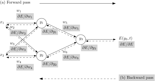
In machine learning, a specialized counterpart of AD known as the backpropagation algorithm has been the mainstay for training neural networks, with a colorful history of having been reinvented at various times by independent researchers (Griewank2012; schmidhuber2015deep). It has been one of the most studied and used training algorithms since the day it became popular mainly through the work of rumelhart1986learning. In simplest terms, backpropagation models learning as gradient descent in neural network weight space, looking for the minima of an objective function. The required gradient is obtained by the backward propagation of the sensitivity of the objective value at the output (Figure 1), utilizing the chain rule to compute partial derivatives of the objective with respect to each weight. The resulting algorithm is essentially equivalent to transforming the network evaluation function composed with the objective function under reverse mode AD, which, as we shall see, actually generalizes the backpropagation idea. Thus, a modest understanding of the mathematics underlying backpropagation provides one with sufficient background for grasping AD techniques.
In this paper we review AD from a machine learning perspective, covering its origins, applications in machine learning, and methods of implementation. Along the way, we also aim to dispel some misconceptions that we believe have impeded wider recognition of AD by the machine learning community. In Section 2 we start by explicating how AD differs from numerical and symbolic differentiation. Section LABEL:SectionPreliminaries gives an introduction to the AD technique and its forward and reverse accumulation modes. Section LABEL:SectionDerivativesAndMachineLearning discusses the role of derivatives in machine learning and examines cases where AD has relevance. Section LABEL:SectionImplementations covers various implementation approaches and general-purpose AD tools, followed by Section LABEL:SectionConclusions where we discuss future directions.
2 What AD Is Not
Without proper introduction, one might assume that AD is either a type of numerical or symbolic differentiation. Confusion can arise because AD does in fact provide numerical values of derivatives (as opposed to derivative expressions) and it does so by using symbolic rules of differentiation (but keeping track of derivative values as opposed to the resulting expressions), giving it a two-sided nature that is partly symbolic and partly numerical (Griewank2003). We start by emphasizing how AD is different from, and in several aspects superior to, these two commonly encountered techniques of computing derivatives.
2.1 AD Is Not Numerical Differentiation
Numerical differentiation is the finite difference approximation of derivatives using values of the original function evaluated at some sample points (Burden2001) (Figure 2, lower right). In its simplest form, it is based on the limit definition of a derivative. For example, for a multivariate function , one can approximate the gradient using
| (1) |
where is the -th unit vector and is a small step size. This has the advantage of being uncomplicated to implement, but the disadvantages of performing evaluations of for a gradient in dimensions and requiring careful consideration in selecting the step size .
Numerical approximations of derivatives are inherently ill-conditioned and unstable,555Using the limit definition of the derivative for finite difference approximation commits both cardinal sins of numerical analysis: “thou shalt not add small numbers to big numbers”, and “thou shalt not subtract numbers which are approximately equal”. with the exception of complex variable methods that are applicable to a limited set of holomorphic functions (Fornberg1981). This is due to the introduction of truncation666Truncation error is the error of approximation, or inaccuracy, one gets from not actually being zero. It is proportional to a power of . and round-off777Round-off error is the inaccuracy one gets from valuable low-order bits of the final answer having to compete for machine-word space with high-order bits of and (Eq. 1), which the computer has to store just until they cancel in the subtraction at the end. Round-off error is inversely proportional to a power of . errors inflicted by the limited precision of computations and the chosen value of the step size . Truncation error tends to zero as . However, as is decreased, round-off error increases and becomes dominant (Figure LABEL:FigureApproximationError).