Autonomous Apple Fruitlet Sizing and Growth Rate Tracking using Computer Vision
Abstract
In this paper, we present a computer vision-based approach to measure the sizes and growth rates of apple fruitlets. Measuring the growth rates of apple fruitlets is important because it allows apple growers to determine when to apply chemical thinners to their crops in order to optimize yield. The current practice of obtaining growth rates involves using calipers to record sizes of fruitlets across multiple days. Due to the number of fruitlets needed to be sized, this method is laborious, time-consuming, and prone to human error. With images collected by a hand-held stereo camera, our system, segments, clusters, and fits ellipses to fruitlets to measure their diameters. The growth rates are then calculated by temporally associating clustered fruitlets across days. We provide quantitative results on data collected in an apple orchard, and demonstrate that our system is able to predict abscise rates within 3.5% of the current method with a 6 times improvement in speed, while requiring significantly less manual effort. Moreover, we provide results on images captured by a robotic system in the field, and discuss the next steps required to make the process fully autonomous.
Index Terms:
Agricultural Automation, Computer Vision for Automation, Robotics in Agriculture and Forestry, Field RoboticsI Introduction
Recent advancements in computer vision have allowed farmers to deploy autonomous plant monitoring solutions to more efficiently inspect vast quantities of crops. Computer vision-based systems provide fast and reliable information for downstream tasks such as harvesting [1, 2], phenotyping [3, 4], and yield prediction [5, 6, 7], ultimately allowing farmers to make real-time crop management decisions. Common computer vision applications in agriculture include mapping [8, 9], counting [10, 11, 12], modelling [13, 14], and disease classification [15].
We focus on the target application of measuring growth rates of apple fruitlets333A fruitlet is a young apple formed on the tree shortly after pollination. This is important because it enables farmers to better control their annual yield. It is standard practice to thin apple trees to prevent them from developing a pattern of alternative year bearing in order to produce a more consistent yearly harvest. To predict the effect of thinning application applied on trees, the Fruitlet Growth Model developed by Greene et al. [16] is used to determine how often farmers need to spray their crops. The model takes into account the growth rates of a subset of fruitlets over multiple days. The fruitlets with growth rates greater than 50% of the fastest growing fruits are predicted to persist the thinning. Farmers calculate the percentage of fruitlets expected to abscise and use this information to determine if another round of chemical thinner needs to be applied.
The sizing method most commonly used in practice involves identifying each individual fruitlet, using a digital caliper to hand-measure sizes, and manually entering the data into a spreadsheet so that growth rates can be tracked. We will refer to this sizing process as the caliper method. The number of fruit typically sized using the caliper method is approximately 400-500 fruitlets per varietal. This means growers need to size hundreds to thousands of fruitlets depending on the number of varietals that they grow. Each fruitlet is sized twice per thinning application: once three to four days after application, and again seven to eight days after application. Taking this many hand-measurements is not only labor-intensive, but highly subject to human error. It is inefficient and time-consuming for a human to record caliper readings for hundreds to thousands of fruitlets across multiple days, making some farmers hesitant to adopt the approach. Manually associating fruitlets across different days is also very challenging; fruitlets are likely to have moved or fallen off, resulting in them being mis-identified which negatively affects growth estimates. Moreover, using calipers creates variability when measuring asymmetrically shaped fruit, leading to inaccurate measurements which become more pronounced as different workers are employed to collect data. As a result, there is a need to automate this process to make sizing faster, more repeatable, and more accurate.
In this paper, we present a computer vision-based system for sizing and measuring the growth rates of apple fruitlets using stereo image pairs generated from a hand-held camera. Our system segments, clusters, and fits ellipses to apple fruitlets to measure their diameters. Fruitlets are autonomously clustered and temporally associated to track growth rates across days. We demonstrate that the results produced by our method are comparable to those produced by the caliper method, with the ability to reduce the labor-intensive effort and significantly improve speed. The specific contributions of this paper are:
-
i
A computer vision-based system to autonomously size and measure growth rates of apple fruitlets
-
ii
Experiments and results on data collected by a hand-held stereo camera in a commercial apple orchard
-
iii
Quantitative evaluation on data collected by a robotic system in a commercial apple orchard
II Related Work
There has been significant work dedicated towards sizing fruit in agriculture. In the work of [6], calibration spheres are placed on trees and used as reference scales to estimate the sizes of segmented apples. Similarly, Wang et al. [17] are able to size fruits in the field with a smartphone by placing a reference circle of known size behind the fruit. While these methods only require simple segmentation and sizing algorithms, they do not extend well to fruitlets as it is impractical to place reference objects behind hundreds of fruit in occluded environments.
Approaches have also been developed to size fruit in 3D. Reconstruction-based methods are used by [18, 19], where 3D models are created from multiple sensor measurements. However, these methods are computationally expensive and do not perform well with occlusions where reconstructions are often incomplete. To address these issues, automated shape completion methods have been implemented by [20, 21] which fit superellipsoids to accumulated point clouds. These methods either rely on successive frame alignment algorithms, such as Iterative Closest Point, which fail in agricultural environments due to the dynamic structure of plants, or use expensive ray casting operations which are slow when performed at finer resolutions. 3D sizing is performed by [22] where the major-axis of an apple is fit to 3D points collected from a single camera image and time-of-flight sensor. However, the performance is poor, achieving an accuracy of 69.1. The work of [23] also sizes apples from single images by fitting spheres in 3D. This would not adapt well to apple fruitlets due to their small size making it challenging to capture enough of the fruit’s surface.
As an alternative to 3D sizing, 2D photogrammetric methods have been adopted in agriculture. These methods either directly estimate the widths of fruits [22] or fit ellipses to measure the heights and widths [24, 25]. This is advantageous as sizes are able to be extracted quickly from 2D images without the need to aggregate information from multiple views. However, the presented approaches use simple detection and segmentation modules, relying on color information and non-deep features. While these methods work well in their respective domains, they would fail when trying to detect and segment fruitlets. This is because the proximity of fruitlets are much closer together, and their colors blend in with the surrounding leaves. Most similar to our approach, the work of Qadri [26] fits ellipses to apple fruitlets to estimate their diameters. However, they make use of a MADNet [27] network to estimate disparity which uses only the left image and requires re-training between stereo cameras. Additionally, they do not provide a method to autonomously cluster and associate fruitlets which is required to calculate growth rates.
III Methodology
III-A System Overview
The Fruitlet Growth Model [16] specifies that growers select the fruitlet clusters444A cluster is a group of fruitlets that grow out of the same bud they want to size and measure the growth rates of all fruitlets in each cluster. Our system is designed to replicate this process by both sizing the fruitlets and autonomously identifying which fruitlets in the image belong to the cluster intended to be sized. We refer to this cluster as the target cluster.
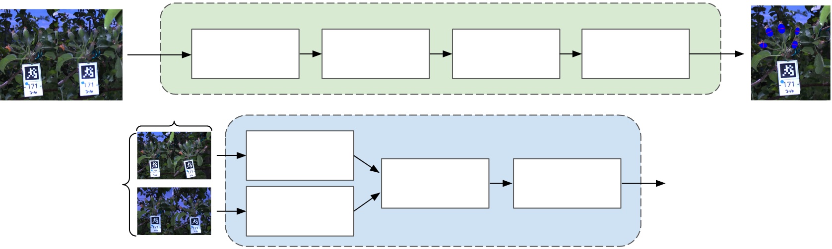
Images are captured in the field using an illumination-invariant flash stereo camera [28]. Once images of all clusters are acquired, the data is passed through our sizing and growth-rate tracking pipelines (Fig. 1). In the first stage, the fruitlets belonging to the target clusters are extracted and sized. All fruitlets in each image are segmented using a Mask-RCNN [29] instance segmentation network, and disparities are extracted using RAFT-Stereo [30] to build point clouds of each fruitlet. The point clouds are used to cluster the fruitlets using a multi-stage Louvain Community Detection [31] approach, and the fruitlets corresponding to the target cluster are identified. Ellipses are fit to the fruitlets that belong to the target cluster, and the diameter of each fruitlet is calculated using the minor axis of the fit ellipse and the disparity values.
The second stage consists of fruit association and growth rate tracking. Fruitlets in images taken in the same and across different days are associated using an approach that makes use of Iterative Closest Point and the Hungarian Algorithm [32]. The sizes of the resulting temporally associated fruitlets are used to calculate growth rates, which in turn are used to predict the percentage of fruitlets that will persist and abscise.
III-B Fruitlet Cluster Sampling
The Fruitlet Growth Model specifies that growers choose the number of trees and the number of clusters per tree they want to size. While the original model suggests using 15 clusters per tree across 7 trees for a total of 105 clusters, we instead use 7 clusters per tree across 10 trees for a total of 70 clusters. This is because using fewer clusters has been previously adopted by apple growers to save time acquiring data. For example, Michigan State University555https://mediaspace.msu.edu/media/How+to+Use+the+Fruit+Growth+Model+to+Guide+Apple+Thinning+Decisions/1_o359pflp and the University of Massachusetts666https://ag.umass.edu/fruit/fact-sheets/hrt-recipe-predicting-fruit-set-using-fruitlet-growth-rate-model suggest using 5 trees with either 15 or 14 clusters per tree respectively. Additionally, spreading clusters over more trees allows us to collect data on a wider range of fruitlet sizes and appearances. This is advantageous as it allows us to evaluate our system’s performance on a more diverse and representative set of fruitlets. Because our objective is to compare predicted thinner response between computer vision and hand-caliper growth rates, and not compare against actual abscise rates, this is a fair sampling strategy for the purpose of this work.
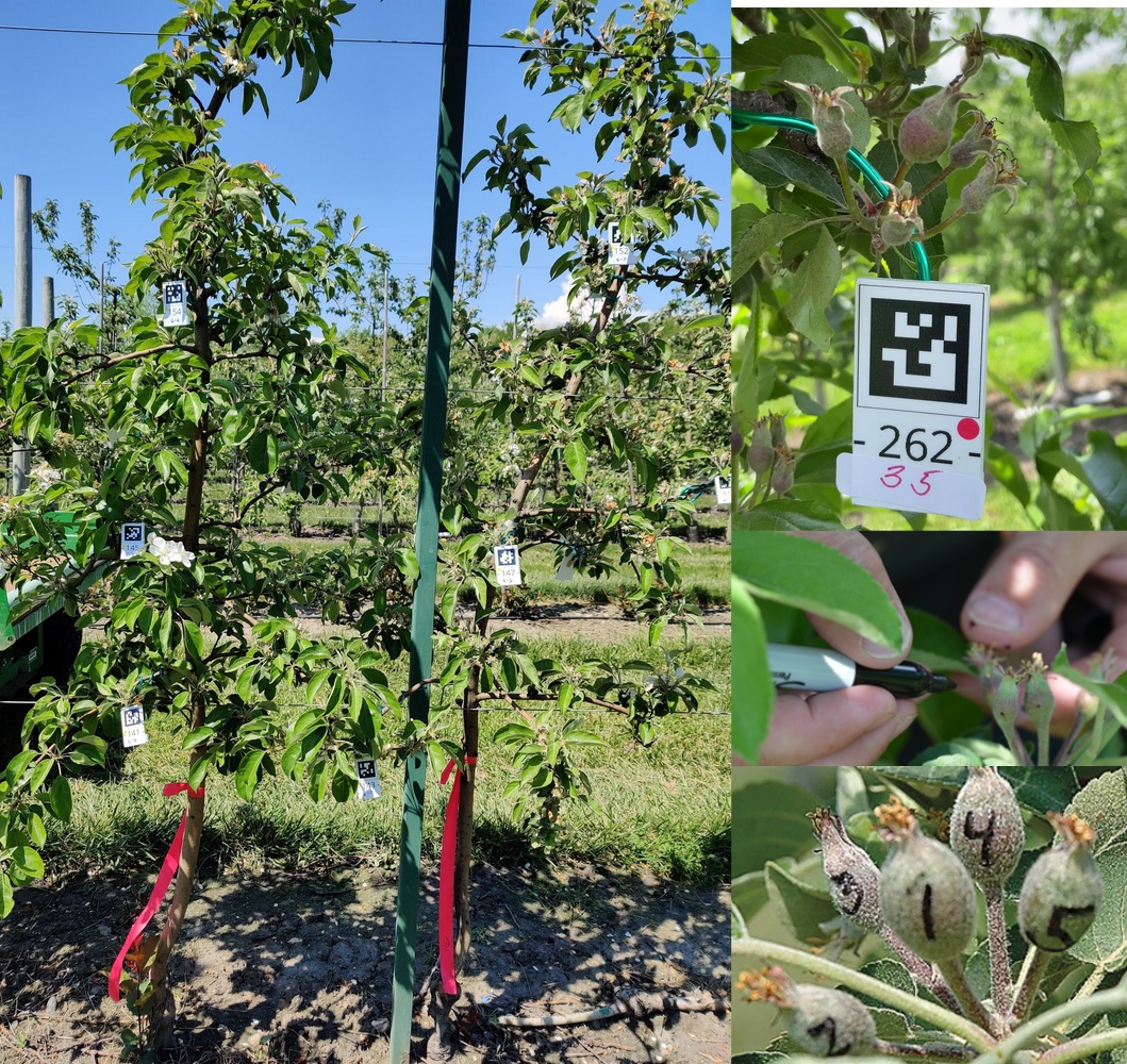
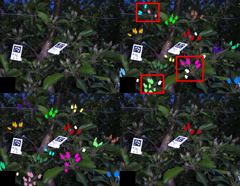
We hang AprilTags [33] to identify the selected clusters and fruitlets. AprilTags were selected because they allow for fast identification in computer vision systems. The AprilTag is only used for identifying the cluster id in addition to determining which fruitlet cluster is the target cluster, as described in Section III-E. Each fruitlet in each cluster is assigned a unique id written on the back which is used for evaluating against ground truth. An example of tagged fruitlet trees and clusters can be seen in Fig. 2.
III-C Image Capture
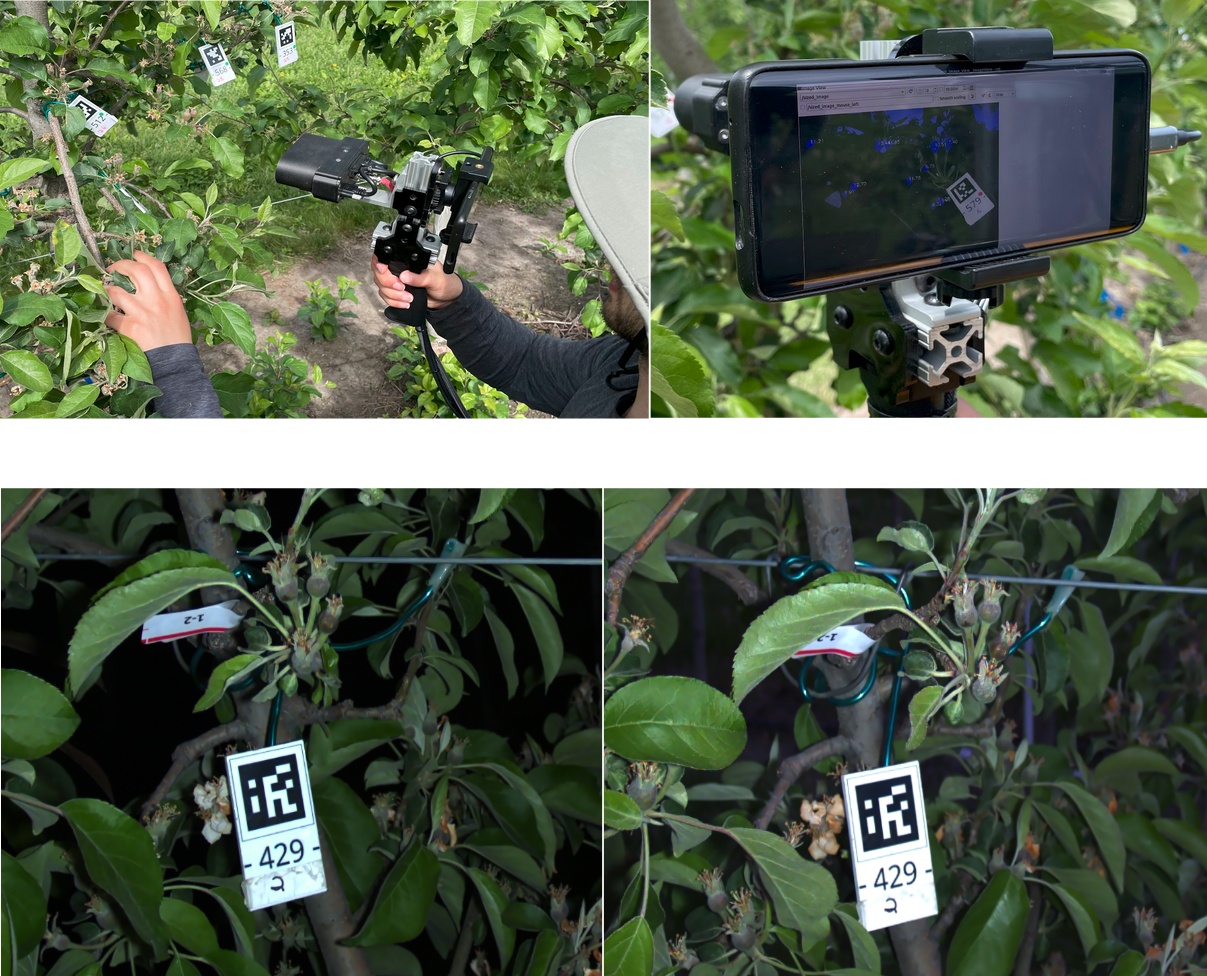
Images are captured using an in-hand version of the illumination-invariant flash stereo camera presented by Silwal et al. [28]. Stereo camera systems are commonly used in agriculture to extract 3D information as a result of their reliability and low cost. They resolve finer details compared to systems that use LiDAR [34, 35, 36], and flash-based systems are more resilient to varying illumination conditions (Fig. 3 c-d) where RGB-D sensors inconsistently perform [24, 22].
To facilitate data collection, we designed a custom setup that consists of the stereo camera connected via USB to a laptop to save the captured images. A phone is mounted on the back and connected via USB-C to the same laptop to allow the user to visualize and assess the quality of the images in real-time. When imaging, one to two images per cluster are captured per day. The reason for this is because we want to limit both the amount of time apple growers need to spend in the field acquiring images and the computational time required to post-process the data. Taking many images or long video sequences significantly adds time to both processes, which results in reduced benefit. Ideally, one image per cluster is taken, but two images are used when not every fruitlet is visible in a single image as a result of occlusions.
III-D Segmentation and Disparity Estimation
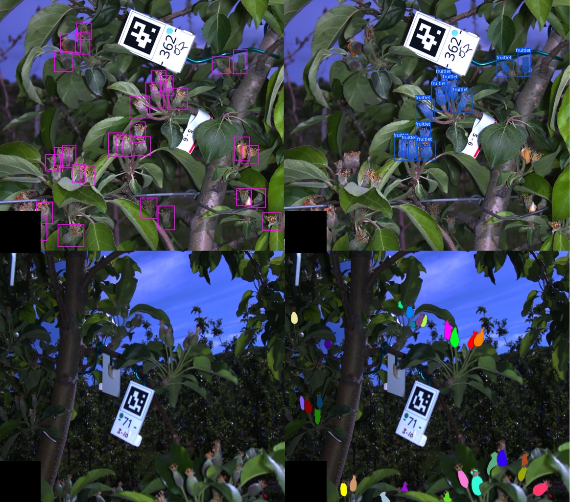
Two differences between our sizing approach and the one presented by Qadri [26] is we replace the MADNet [27] disparity and pix2pix [37] segmentation networks with RAFT-Stereo [30] and Mask-RCNN [29] respectively. RAFT-Stereo is a state-of-the-art deep learning-based stereo matching network that outperforms traditional disparity generation methods, such as SGBM [38], on benchmarks such as the Middleburry Stereo Evaluation777https://vision.middlebury.edu/stereo/eval3/. Additionally, RAFT-Stereo does not require fine-tuning, which is advantageous as the network does not need to be retrained between datasets or when switching out the stereo camera being used. In addition, Mask-RCNN is a more standard and widely adopted instance segmentation network compared to pix2pix, which is traditionally used for pair-to-pair image translation.
To account for the difficulties in obtaining ground truth segmented data, the Mask-RCNN network is trained following a two stage process. In the first stage, bounding box annotations are used to train the bounding box regression and classification heads. In the second stage, the weights of these heads are frozen, and a subset of the fruitlets in each image are segmented and used to train the mask head. An overview of the process can be seen in Fig. 4. We use a customized detectron2 [39] Mask-RCNN implementation.
III-E Fruitlet Clustering
In order to measure and compare the growth rates of the fruitlets, our system needs to be able to identify which fruitlets belong to the target cluster. We achieve this using a multi-stage Louvain Community Detection [31] approach. Louvain Community Detection is an algorithm that extracts communities within a graph using a heuristic method based on modularity optimization. A community is a subset of nodes whose connections among themselves are denser than connections with the rest of the graph. The algorithm iterates through nodes and moves each node into the community that maximizes modularity gain. The process repeats for each node until no modularity gain can be found. We use the NetworkX [40] Louvain Community Detection implementation.
Point clouds of each fruitlet are first extracted using the segmentations and disparities from Section III-D. The point clouds are filtered using a bilateral filter and a depth discontinuity filter [41]. Point clouds with too few points or inconsistent depth values are discarded.
Input:
Parameters: , , ,
Output:
We then perform our clustering approach as described in Algorithm 1. We first construct a graph consisting of the centroids of each fruitlet as a node. An edge is created between nodes if their euclidean distance is less than a pre-determined threshold . The weight of edge is determined based on the euclidean distance, with closer nodes receiving a greater edge weight. Louvain Community Detection (LCD in Algorithm 1) is then run on to produce a set of communities .
As a result of the inconsistent spacings between fruitlets and fruitlets falling off during the thinning period, naively using only Louvain Community Detection often results in fruitlet clusters being incorrectly divided into multiple communities (Fig. 5 (b)). We observed that when this occurs one of the communities almost always contains two fruitlets. To account for this, we iterate through all communities of size two and combine them with their nearest communities if the distance between the centroids of all the fruitlets in the combined community and the centroid of the combined community is less than a threshold (MergeCommunities in Algorithm 1).
There are occasionally clusters all of whose fruitlets are unassigned to a community. To overcome this, we repeat the above process for all unassigned fruitlets using a relaxed threshold. A graph is built consisting of the unassigned fruitlet centroids, and edges and weights are created as before with a new threshold . Louvain Community Detection is run on this graph to produce a new set of communities , which is combined with to form . Once again, communities of size two are merged. As a final step, all remaining unassigned fruitlets are merged with their nearest communities (MergeUnassigned in Algorithm 1) if the distance between the centroids of all the fruitlets in the combined community and the centroid of the combined community is less than . A visualization of the final result can be seen in Fig. 5 (c). The fruitlets belonging to the community closest to the AprilTag are determined to belong to the target cluster and are used for sizing and growth rate tracking (Fig. 5 (d)).
III-F Ellipse Fitting and Sizing
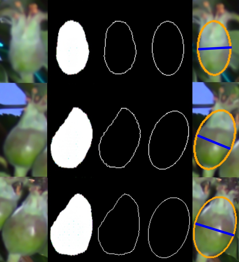
An ellipse is fit to the segmented fruitlets in the target cluster following the process demonstrated in Fig. 6. First, for each fruitlet in the target cluster, the contour surrounding the segmented points is extracted. Then, an ellipse is fit using the OpenCV [42] fitEllipse function. Finally, the size is calculated as , where is the baseline of the stereo camera, is the median disparity value of the segmented pixels, and is the length of the minor axis of the fit ellipse. The derivation for this equation can be found in [26].
III-G Growth Rate Tracking
While the sizing pipeline presented in Fig. 1 (a) automates the fruitlet sizing process by removing the need for hand-caliper measurements, the fruitlets still need to be associated between images taken on the same and across different days in order to measure growth rates. We accomplish this by using a coarse cluster alignment to fine fruitlet matching approach. First, for each image, a point cloud of the target cluster is created by combing the point clouds of the individual fruitlets. Iterative Closest Point is run on the cluster point clouds to align them. The fruitlets are then associated using the Hungarian algorithm [32] on the pairwise euclidean distances of their transformed centroids. Matches whose euclidean distance exceeds a specified threshold are discarded. This simple matching method provides reasonable performance to predict persist and abscise percentages.
As demonstrated in Fig. 1 (b), the fruitlets are first associated in images taken on the same day, and the larger size of each fruitlet is used for calculating growth rates. If only one image is taken of a cluster on a particular day, this step is skipped. Next, the fruitlets are temporally associated across days and growth rates are calculated by finding the difference between the end and start sizes.
Lastly, thinner response in the form of persist and abscise rates are predicted following the process described in the Fruitlet Growth Model [16]. This is achieved by calculating the average growth rate of the top 20 fastest growing fruitlets. All fruitlets with growths rates greater than 50% of this value are predicted to persist, and the rest abscise. We validate our calculations by comparing our results to those produced by the Predicting Fruitset spreadsheet available at the Michigan State University Extension Horticulture website 888https://www.canr.msu.edu/apples/horticulture/.
| 2021 | 2022 | 2023 | |||||||
| Day 1 | 05/21/2021 | 05/22/2022 | 05/19/2023 | ||||||
| Day 3 | 05/23/2021 | 05/24/2022 | 05/21/2023 | ||||||
| Day 5 | 05/25/2021 | 05/26/2022 | Freeze Occurred | ||||||
| Varietal | Fuji | Gala | Honeycrisp | Fuji | Gala | Honeycrisp | Honeycrisp | ||
| Total Clusters | 84 | 84 | 84 | 70 | 70 | 70 | 70 | ||
| Train Clusters | 14 | 14 | 14 | 0 | 0 | 0 | 70 | ||
| Eval Clusters | 70 | 70 | 70 | 70 | 70 | 70 | 0 | ||
| Total Train Clusters: | 112 | ||||||||
| Total Eval Clusters: | 420 | ||||||||
IV Experiments
IV-A Dataset
Our datasets will be made publicly available at 999https://labs.ri.cmu.edu/aiira/resources/ by the time of publication.
IV-A1 Data Collection
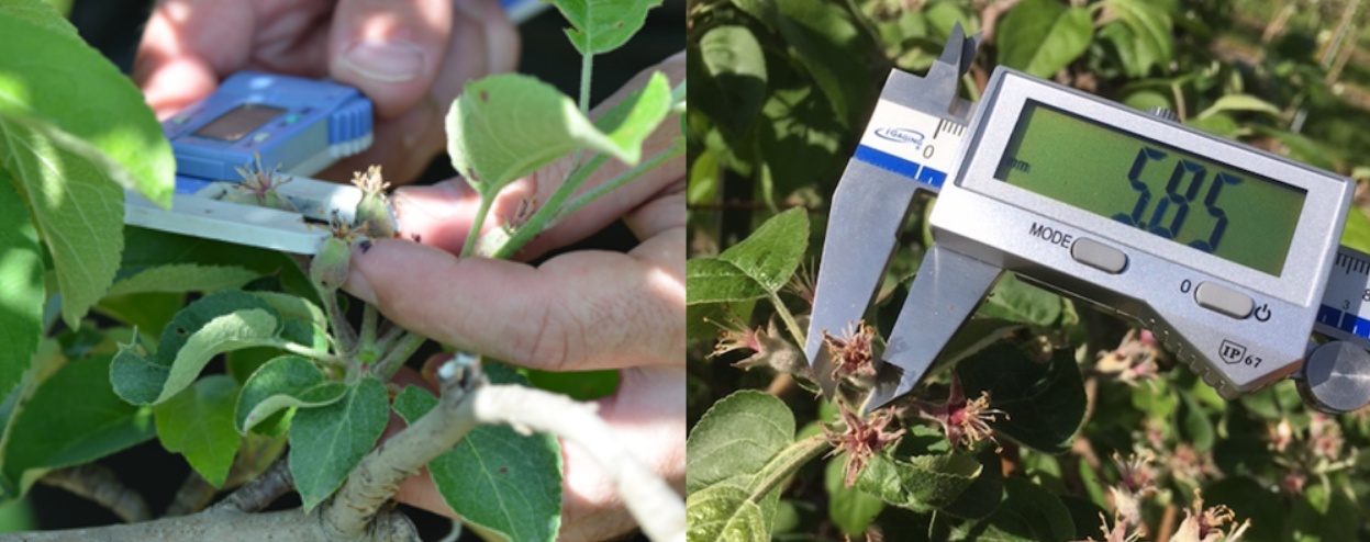
Our dataset consists of stereo-images of 532 clusters along with their respective caliper measurements collected over three years. The data was collected at the University of Massachusetts Amherst Cold Spring Orchard. Each cluster was imaged three times over a period of five days, represented as Day 1, Day 3, and Day 5. The breakdown of dates and varietals can be seen in Table I. Prior to data collection, the clusters were selected and tagged with an AprilTag and the fruitlets were individually labelled following the process described in Section III-B. A human manually operated the hand-held stereo camera (Fig. 3), collecting a sequence of images of each cluster. For evaluation, one to two images from each cluster per day were manually selected, representing an apple grower taking one to two images as described in Section III-C. Hand measurements were collected for each fruitlet using a digital caliper (Fig. 7).
Taking measurements with calipers naturally results in random errors. This is because the measurement will very as the caliper is rotated around the fruitlet as a result of its asymmetrical shape. As well, the measurements are dependant on how hard the caliper is closed around the fruitlet, which can easily change from day to day and from person to person. To quantitatively asses this variation, we collected 45 fruitlets equally distributed between small ( 8mm), medium ( 8mm and 12mm) and large ( 12mm) sizes. For each fruitlet, we measured its diameter 5 times using calipers, and recorded the difference between the maximum and minimum sizes. The average difference for the small, medium, and large fruitlets were 0.50mm, 0.34mm, and 0.71mm respectively. The maximum differences were 2.31mm, 0.52mm, and 1.85mm respectively. These measurement inconsistencies further demonstrate the need for alternative solutions.
IV-A2 Train and Evaluation Splits
All imaged clusters were split into training and evaluation clusters, as shown in Table I. The training clusters were use to train and validate the Mask-RCNN network as well as tune the parameters for fruitlet clustering. As discussed in Section III-B, because we use 70 clusters to predict thinning response, 14 of the 84 clusters per varietal imaged in 2021 were used for training, and the rest were used for evaluation. Additionally, a freeze occurred during our data collection in 2023, effectively ending the growth of the fruitlets. As a result, clusters imaged in 2023 were used for training. All clusters imaged in 2022 were used for evaluation, which demonstrates our method’s ability to generalize to datasets taken on different years without requiring the need to fine tune any of the models. The final evaluation data includes 6 sets of 70 clusters evenly distributed over 2021 and 2022 fuji, gala, and honeycrisp varietals.
IV-A3 Annotation Labelling
To train the Mask-RCNN network, 600 images were randomly selected from the images of the training clusters. Bounding boxes were labelled around every fruitlet to train the Mask-RCNN bounding box classification and regression heads, as discussed in Section III-D. From the 600 images, 100 were randomly selected and used to manually hand segment 1000 fruitlets to train the mask head. All data was then divided into training, validation, and test sets to train the network, with a 70/15/15 split respectively.
IV-B Fruitlet Sizing
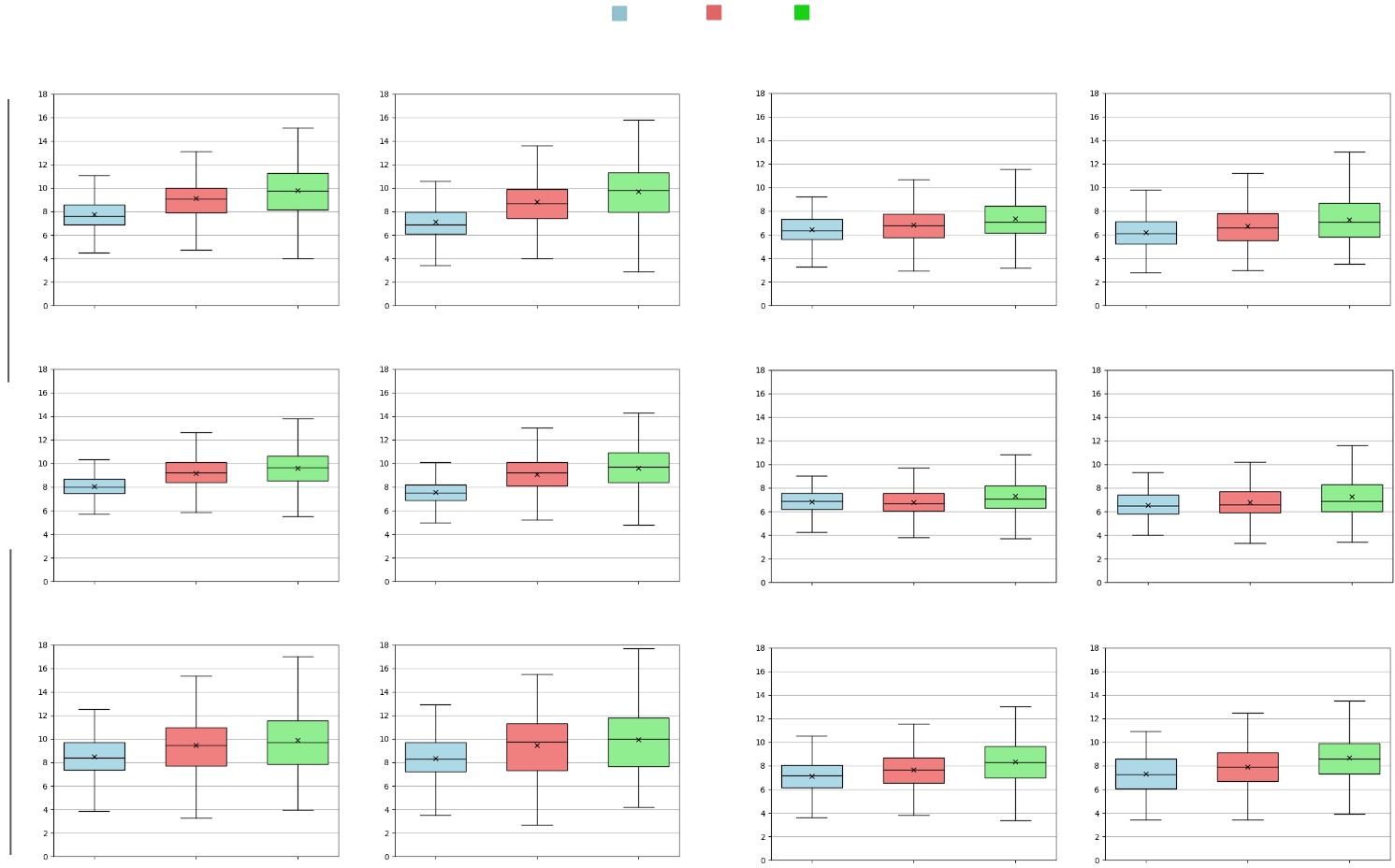
We evaluate our fruitlet sizing approach. After all fruitlets are sized, outliers are removed from our computer vision pipeline using a Z-score with threshold 3. The number of outliers removed is less than 0.25% of all fruitlets sized. The distribution of measured sizes using our computer vision sizing pipeline (CVSP) and the ground truth caliper measurements (GT) are reported Fig. 8. While the computer vision pipeline produces slightly larger results on Day 1 for most datasets, the size and growth trends are similar across the 5 day period with regards to mean, median, and size distribution.
| 2021 | 2022 | |||||||||||||||||||||||
|---|---|---|---|---|---|---|---|---|---|---|---|---|---|---|---|---|---|---|---|---|---|---|---|---|
| Fuji | Gala | Honeycrisp | Fuji | Gala | Honeycrisp | |||||||||||||||||||
| Day 1 | Day 3 | Day 5 | All | Day 1 | Day 3 | Day 5 | All | Day 1 | Day 3 | Day 5 | All | Day 1 | Day 3 | Day 5 | All | Day 1 | Day 3 | Day 5 | All | Day 1 | Day 3 | Day 5 | All | |
| CVSP (ours) | ||||||||||||||||||||||||
| MAE (mm) | 0.771 | 0.582 | 0.607 | 0.652 | 0.645 | 0.607 | 0.661 | 0.642 | 0.603 | 0.672 | 0.714 | 0.662 | 0.610 | 0.580 | 0.602 | 0.597 | 0.650 | 0.625 | 0.585 | 0.616 | 0.701 | 0.721 | 0.792 | 0.739 |
| MAPE (%) | 12.1 | 7.27 | 7.57 | 8.98 | 9.02 | 7.24 | 7.28 | 7.92 | 8.40 | 8.33 | 7.99 | 8.26 | 11.51 | 9.64 | 9.41 | 10.22 | 10.5 | 9.61 | 8.60 | 9.57 | 10.06 | 9.88 | 9.86 | 9.98 |
| % Sized | 83.6 | 90.4 | 87.9 | 87.4 | 95.6 | 95.4 | 95.3 | 95.2 | 95.4 | 96.0 | 96.8 | 95.7 | 81.3 | 86.7 | 88.2 | 84.9 | 88.1 | 93.9 | 94.5 | 91.9 | 95.3 | 93.8 | 95.5 | 94.7 |
| Score | 0.830 | 0.889 | 0.896 | 0.899 | 0.587 | 0.722 | 0.739 | 0.748 | 0.854 | 0.858 | 0.875 | 0.869 | 0.729 | 0.779 | 0.845 | 0.796 | 0.570 | 0.671 | 0.842 | 0.724 | 0.610 | 0.713 | 0.772 | 0.731 |
| SGBM-CVSP | ||||||||||||||||||||||||
| MAE (mm) | 0.708 | 1.08 | 1.19 | 0.994 | 0.955 | 1.19 | 1.48 | 1.21 | 1.01 | 1.40 | 1.40 | 1.27 | 0.593 | 0.596 | 0.652 | 0.604 | 0.871 | 0.903 | 0.790 | 0.849 | 0.767 | 0.718 | 0.731 | 0.743 |
| MAPE (%) | 10.6 | 12.0 | 12.7 | 11.8 | 12.7 | 13.1 | 14.9 | 13.5 | 12.0 | 14.7 | 13.2 | 13.3 | 10.8 | 9.44 | 9.51 | 9.89 | 12.9 | 13.5 | 11.3 | 12.5 | 10.7 | 9.22 | 8.54 | 9.57 |
| % Sized | 82.9 | 87.2 | 84.6 | 84.6 | 94.5 | 91.3 | 91.5 | 92.3 | 92.7 | 92.8 | 91.1 | 96.2 | 54.8 | 40.6 | 52.9 | 49.0 | 35.6 | 42.6 | 53.1 | 43.7 | 54.8 | 54.8 | 52.6 | 53.4 |
| Score | 0.695 | 0.596 | 0.700 | 0.694 | 0.243 | 0.369 | 0.401 | 0.417 | 0.602 | 0.624 | 0.672 | 0.638 | 0.687 | 0.804 | 0.809 | 0.800 | 0.486 | 0.492 | 0.662 | 0.560 | 0.565 | 0.723 | 0.796 | 0.732 |
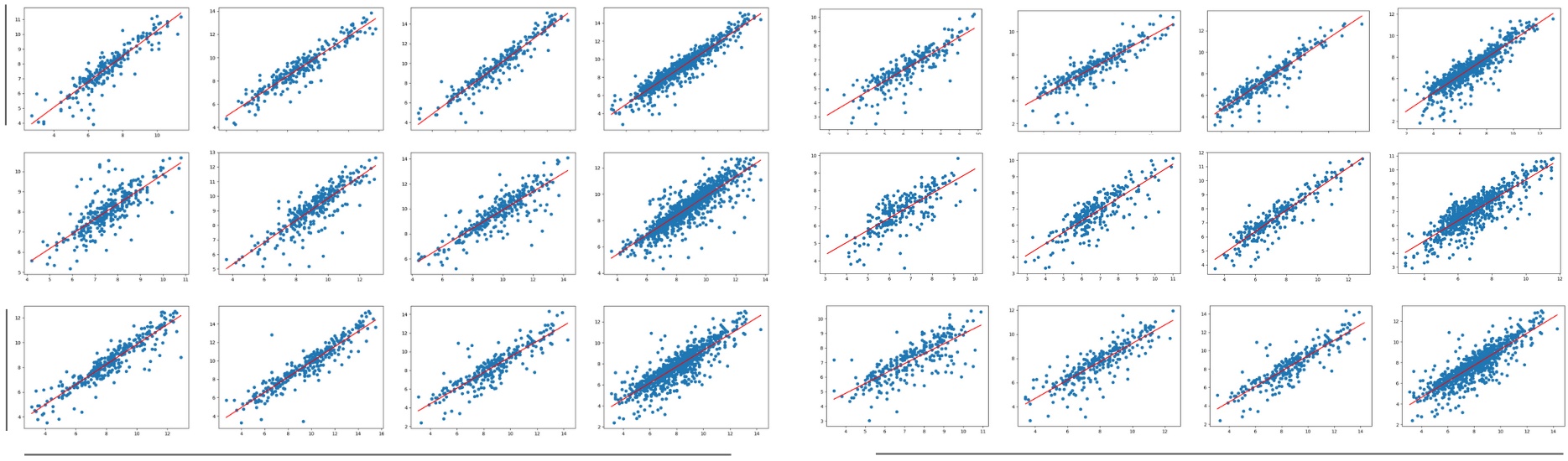
Table II shows the Mean Absolute Error (MAE), the Mean Absolute Percentage Error (MAPE), the percentage of fruitlets sized, and the linear fit score of the computer vision sizes compared against the caliper method for each day, as well as across all days. All linear fit plots can be seen in in Fig. 12. The MAE is consistently under 1mm, and the MAPE remains below 10% except for on the first day of the Fuji 2021, Fuji 2022, Gala 2022, and Honeycrisp 2022 varietals. Additionally, we are able to size approximately 85% - 95% of fruitlets, and achieve scores between 0.724 and 0.899 across all days.
As expected, fruitless sized on the first day typically have a higher MAPE and lower score compared to the later days. One possible reason for this is because is it more difficult to accurately segment smaller fruitlets as their flowery top covers a greater percentage of the fruit. On the other hand, the errors may stem from the inconsistencies in measuring ground truth. The size variations from using calipers would have a more significant effect when the fruitlets are small.
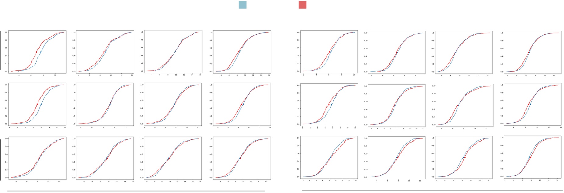
We also plot the cumulative distribution functions (CDF) of fruitlet sizes in Fig. 12. The CDFs follow similar shapes across all varietals and days. The most noticeable difference is on Day 1 for most varietals, where there is a horizontal shift between the CVSP and ground truth distributions. This is again because of the difficulty in sizing smaller fruit.
We also investigate the effect of replacing RAFT-Stereo with the classical disparity estimation method SGBM [38] (SGBM-CVSP). As shown in Table II, fewer fruitlets are able to be sized using SGBM, especially for the fruitlets imaged in 2022. When a similar number of fruitlets are able to be sized (the 2021 varietals), using SGBM results in higher MAE and MAPE values and lower scores. These results are likely because SGBM is unable to assign a disparity value to every pixel. As well, the performance of its disparity estimation is sensitive to the algorithm parameters used.
| Mean (s) | Median (s) | Std (s) | |
|---|---|---|---|
| RAFT-Stereo | 4.32 | 4.29 | 0.226 |
| Mask-RCNN | 0.225 | 0.220 | 0.0719 |
| Fruitlet Clustering | 0.190 | 0.190 | 0.00907 |
| Sizing | 0.00617 | 0.00603 | 0.00258 |
| Total | 4.74 | 4.71 | 0.248 |
We assess the speed of our sizing pipeline. Table III shows the distribution of sizing times from image input to sizing output. We ran our evaluation on an NVIDIA GeForce RTX 3070 GPU. The average processing time is approximately 4.74s, with RAFT-Stereo consuming a majority of the time with an average of 4.32s. The speed of RAFT-Stereo and the pipeline will be affected by the GPU used.
We asked apple growers how long it usually takes to size fruitlets with calipers. The response we received is that it takes approximately 30s per cluster, which we confirmed when collecting ground truth measurements. Based on this preliminary study, our computer vision pipeline was able to size fruitlets 6 times faster compared to hand-caliper measurements. We plan to evaluate this performance improvement on a larger scale in the future.
IV-C Fruitlet Association and Thinner Response Prediction
We evaluate the performance of our fruitlet association method and the ability for our full Fruitlet Growth Measurement Pipeline (FGMP) to predict persist and abscise rates. We also evaluate our pipeline against one that uses the classical disparity estimation method SGBM instead of RAFT-Stereo (SGBM-FGMP), and one that naively associates fruitlets based solely on order of size (Size-FGMP). This association method is often done in practice when growers use the modified Ferri Version of the Fruitlet Growth Model 101010https://ag.umass.edu/sites/ag.umass.edu/files/fruit/predictingfruitsetmodelferri.pdf and apps such as Malusim 111111https://malusim.org/ in order to save time from having to manually associate fruitlets. The full results can be seen in Table IV. We compare each method’s ability to predict fruitlet persist and abscise rates with assumed known associations (KA Persist / Abscise %) and compare the absolute abscise percentage difference (KA AAPD) against ground truth. Additionally, we evaluate the precision and recall performance of the association method used in addition to the performance of the full end-to-end pipeline with regards to predicted thinning response (E2E Persist / Abscise %) compared against ground truth (E2E AAPD). Because the only difference between FGMP and Size-FGMP is the association method, both will have the same KA Persist / Absicse % and KA AAPD values. These are reported only in the FGMP section of Table IV. Known and E2E association results are provided to demonstrate the performance should the grower choose to manually or autonomously associate the fruitlets respectively.
Among the six clusters, our method achieves the lowest average absolute percentage difference compared to ground truth using both known associations and the full end-to-end pipeline, with 3.75% and 3.33% average KA AAPD and E2E AAPD respectively. This is what best demonstrates the effectiveness of our approach. Apple growers would be able to draw similar conclusions about when to spray using our automated pipeline that does not require any manual sizing or fruitlet identification. Additionally, associating by size also achieves reasonable performance, with an average E2E AAPD of 4.52%. Replacing RAFT with SGBM performed the worst. The SGBM-FGMP pipeline acheived an average KA AAPD and E2E AAPD of 10.5% and 10.9% respectively, with AAPD values greater than 15% for both the 2021 datasets of the Fuji and Gala varietals.
Our method is also able to associate fruitlets with an average precision and recall of 92.2% and 76.1% across all datasets. This is reasonable given the simplicity of the approach. The results suggest that association performance does not have the most significant effect on the pipeline’s ability to estimate abscise rates, as the Size-FGMP method is able to produce reasonable predictions with average association precision and recall values of 46.1% and 43.6%. While more sophisticated deep-learning and slam-based methods may improve association, the small improvement in abscise predication might not be worth the additional computation time and loss of generalizability that our method provides.
| 2021 | 2022 | |||||||
| Fuji | Gala | Honeycrisp | Fuji | Gala | Honeycrisp | Average | ||
| GT Persist / Abscise % | 53.0 / 47.0 | 48.0 / 52.0 | 27.2 / 72.8 | 37.2 / 62.8 | 27.5 / 72.5 | 42.4 / 57.6 | x | |
| FGMP (ours) | KA Persist / Abscise % | 50.7 / 49.3 | 41.4 / 58.6 | 26.0 / 74.0 | 38.0 / 62.0 | 22.9 / 77.1 | 35.4 / 65.6 | x |
| KA AAPD (%) | 2.3 | 6.6 | 1.2 | 0.8 | 4.6 | 7.0 | 3.75 | |
| Association Precision | 95.1 | 92.9 | 96.4 | 86.4 | 89.2 | 93.0 | 92.2 | |
| Association Recall | 74.7 | 83.4 | 86.1 | 62.6 | 70.8 | 79.2 | 76.1 | |
| E2E Persist / Abscise % | 52.3 / 47.7 | 43.6 / 56.4 | 25.0 / 75.0 | 39.4 / 60.6 | 22.2 / 77.8 | 37.4 / 62.6 | x | |
| E2E AAPD (%) | 0.7 | 4.4 | 2.2 | 2.2 | 5.5 | 5.0 | 3.33 | |
| SGBM-FGMP | KA Persist / Abscise % | 34.6 / 65.4 | 24.5 / 75.5 | 21.4 / 78.6 | 38.9 / 61.1 | 34.5 / 65.5 | 48.9 / 51.1 | x |
| KA AAPD (%) | 18.4 | 23.5 | 5.8 | 1.7 | 7.0 | 6.5 | 10.5 | |
| Association Precision | 95.1 | 92.1 | 95.0 | 83.9 | 57.9 | 77.4 | 83.6 | |
| Association Recall | 74.7 | 78.6 | 79.1 | 20.6 | 11.4 | 21.1 | 47.6 | |
| E2E Persist / Abscise % | 35.1 / 64.9 | 24.0 / 76.0 | 22.8 / 77.2 | 40.5 / 59.5 | 38.6 / 61.4 | 46.8 / 53.2 | x | |
| E2E AAPD (%) | 17.9 | 24.0 | 4.4 | 3.3 | 11.1 | 4.4 | 10.9 | |
| Size-FGMP | Association Precision | 53.4 | 35.3 | 49.8 | 49.6 | 35.8 | 42.6 | 46.1 |
| Association Recall | 50.3 | 34.6 | 48.6 | 43.2 | 35.1 | 41.3 | 43.6 | |
| E2E Persist / Abscise % | 52.1 / 47.9 | 44.3 / 55.7 | 24.6 / 75.4 | 42.4 / 57.6 | 24.6 / 75.4 | 34.2 / 65.8 | x | |
| E2E AAPD (%) | 0.9 | 3.7 | 2.6 | 5.2 | 2.9 | 10.2 | 4.52 |
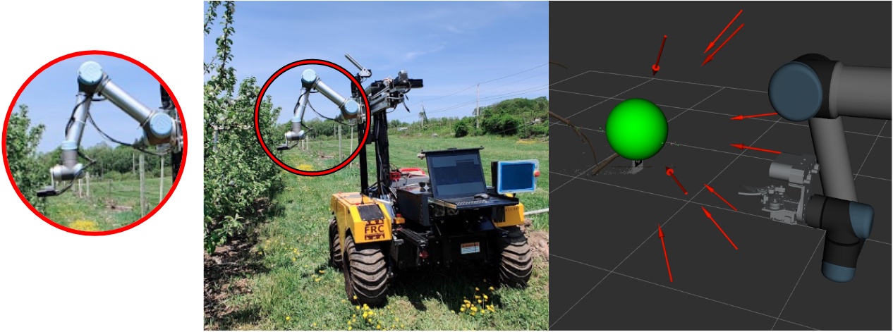
IV-D Robot Experiment
We test our sizing pipeline on images collected by a robotic system in the field. The flash stereo camera is is attached to a 7 DoF robotic arm consisting of a UR5 and linear slider [43]. Images of 30 gala clusters were taken at the University of Massachusetts Amherst Cold Spring Orchard on 3 different days spanning a five day window: 05/22/2022, 05/24/2022, and 05/26/2022, which we denote as Day 1, Day 3, and Day 5 respectively. The robot was controlled to follow a predefined semi-spherical motion path around the detected AprilTag, collecting images at viewpoints equally distributed throughout the motion path (Fig. 9). For each cluster on each day, the two images with the greatest fruitlet segmented area of the target cluster were used to size and calculate growth rates.
The same process described in Section III was used to size the fruitlets. When associating, Iterative Closest Point was still used to correct noise in the robot extrinsics, and fruitlets belonging to the detected target cluster were matched using the Hungarian algorithm on point cloud centroids.
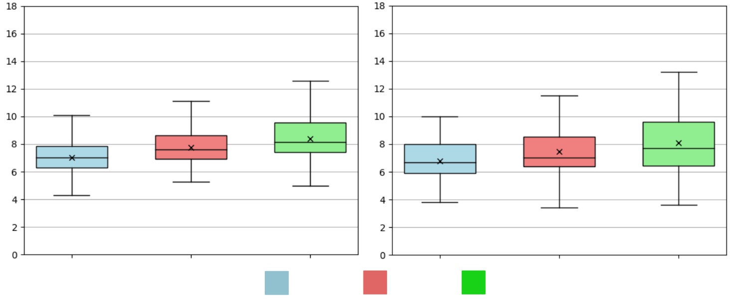
We record the size distributions (Fig. 10) for measurements taken by both our computer vision sizing pipeline with robot captured images (RCVSP) and the caliper method (GT). Across all days, the sizes produced by the computer vision pipeline are larger on average than those produced by the caliper method, and the distributions are much narrower. This is because the robot is naively following pre-set path and not reasoning about where to capture an image. As a result, smaller fruitlets are likely to be completely occluded and unsized.
The MAE, MAPE, and percentage of fruitlets sized are presented in Table V. While the MAE remains under 1mm, the MAPE is higher on average compared to the hand-held camera results presented in Section IV-B. This is because of the partial occlusion of the fruitlets in the images as a result of following the pre-set path. Additionally, the percentage of fruitlets sized decreases as time goes on. This is a result of the larger fruitlets fully occluding the smaller ones, which has a more significant effect as the fruitlets grow.
| Day 1 | Day 3 | Day 5 | All | |
|---|---|---|---|---|
| MAE (mm) | 0.863 | 0.838 | 0.992 | 0.898 |
| MAPE (%) | 14.6 | 12.6 | 13.3 | 13.6 |
| % Sized (mm) | 91.5 | 88.9 | 81.6 | 87.2 |
V Conclusion
This paper presents an alternative approach to sizing and measuring the growth rates of apple fruitlets. We have demonstrated that our computer vision-based method is able to produce similar sizes and thinner response predictions as the current caliper method used in practice. Most notably, we are able to predict similar abscise rates with only one to two single stereo image pairs per cluster, without any human effort required to label fruitlets or take caliper measurements. The advantage our system brings is a faster and less labor intensive approach that produces comparable results.
While our approach produces promising results, there is still work needed in order to make it adoptable by growers. For one, it requires the use of a stereo camera that is able to take quality images in light varying environments. We used a custom-made illumination-invariant camera system [28] that is not freely available. As well, to process results in real-time, a computationally sufficient device has to be carried out in the field and remain connected to the camera. This brings challenges as the wiring makes it difficult to maneuver around the cluster. In an ideal scenario, lightweight models small enough to run mobile devices would be used. While it is possible to replace the backbone of Mask-RCNN with lightweight networks [44, 45], RAFT-Stereo still requires sufficient computational resources. Further investigation is needed to determine if faster learning-based stereo matching algorithms [46, 47] provide sufficient performance to be used in agriculture. Alternatively, one advantage to our fully automated approach is images can be collected and processed offline. This would require connecting the camera to a device with sufficient memory capacity to save the captured images to be processed at a future point in time. Lastly, one drawback of our approach is the system cannot distinguish between a fruitlet that fell off and a missed detection. This affects thinner response predictions as the Fruitlet Growth Model considers fruitlets that have abscised during the sizing period. Future work would have to be dedicated towards distinguishing between these scenarios in order to fully replicate the process described in the model.
The next step to make the process fully autonomous is to replace the need for humans to collect images. This paper evaluates the sizing performance of images collected by a robot following a set motion path. The system fails to successfully size smaller, fully occluded fruitlets and large, partially occluded fruitlets. This is because the robot is not reasoning about the environment as it captures images, unlike a human is with the hand-held camera. While one possible solution to handle partial occlusions is to incorporate the work of Dong et al. [48] to directly infer ellipses, this would require labelling copious amounts of training data that would likely have to be repeated across datasets. As well, this would not handle the case of fully occluded fruits.
In our future work, we focus on integrating next-best-view planning for the task of fully automated fruitlet sizing. This will allow the robot to be able to take high quality images of all fruitlets in the cluster. Recently, there has been work dedicated towards next-best-view planning for fruit sizing using region of interest exploration [21, 49, 50], but these approaches rely on low resolution 3D maps that are insufficient to size fruitlets. As well, sizing is performed by fitting 3D shapes, which is challenging for apple fruitlets because of their small size and often only having one side of their surfaces visible as a result of the occluded environment. We will build upon these works by adapting next-best-view planning techniques to the fruitlet domain and by integrating both 3D and 2D sizing techniques.
Acknowledgments
We would like to thank the University of Massachusetts Amherst Cold Spring Orchard for allowing us to collect data. This research was funded by NSF / USDA NIFA 2020-01469-1022394 and NSF Robust Intelligence 195616.
References
- [1] D. Font, T. Pallejà, M. Tresanchez, D. Runcan, J. Moreno, D. Martínez, M. Teixidó, and J. Palacín, “A proposal for automatic fruit harvesting by combining a low cost stereovision camera and a robotic arm,” Sensors, vol. 14, no. 7, pp. 11 557–11 579, 2014. [Online]. Available: https://www.mdpi.com/1424-8220/14/7/11557
- [2] C. McCool, I. Sa, F. Dayoub, C. Lehnert, T. Perez, and B. Upcroft, “Visual detection of occluded crop: For automated harvesting,” in 2016 IEEE International Conference on Robotics and Automation (ICRA), 2016, pp. 2506–2512.
- [3] S. Paulus, J. Behmann, A.-K. Mahlein, L. Plümer, and H. Kuhlmann, “Low-cost 3d systems: Suitable tools for plant phenotyping,” Sensors, vol. 14, no. 2, pp. 3001–3018, 2014. [Online]. Available: https://www.mdpi.com/1424-8220/14/2/3001
- [4] A. L. Chandra, S. V. Desai, W. Guo, and V. N. Balasubramanian, “Computer vision with deep learning for plant phenotyping in agriculture: A survey,” CoRR, vol. abs/2006.11391, 2020. [Online]. Available: https://arxiv.org/abs/2006.11391
- [5] S. T. Nuske, K. Wilshusen, S. Achar, L. Yoder, S. G. Narasimhan, and S. Singh, “Automated visual yield estimation in vineyards,” J. Field Robotics, vol. 31, pp. 837–860, 2014.
- [6] H. Cheng, L. Damerow, Y. Sun, and M. Blanke, “Early yield prediction using image analysis of apple fruit and tree canopy features with neural networks,” Journal of Imaging, vol. 3, no. 1, 2017. [Online]. Available: https://www.mdpi.com/2313-433X/3/1/6
- [7] B. Darwin, P. Dharmaraj, S. Prince, D. E. Popescu, and D. J. Hemanth, “Recognition of bloom/yield in crop images using deep learning models for smart agriculture: A review,” Agronomy, vol. 11, no. 4, 2021. [Online]. Available: https://www.mdpi.com/2073-4395/11/4/646
- [8] M. Stein, S. Bargoti, and J. Underwood, “Image based mango fruit detection, localisation and yield estimation using multiple view geometry,” Sensors, vol. 16, no. 11, p. 1915, 2016.
- [9] X. Liu, S. W. Chen, C. Liu, S. S. Shivakumar, J. Das, C. J. Taylor, J. Underwood, and V. Kumar, “Monocular camera based fruit counting and mapping with semantic data association,” IEEE Robotics and Automation Letters, vol. 4, no. 3, pp. 2296–2303, 2019.
- [10] W. Qureshi, A. Payne, K. Walsh, R. Linker, O. Cohen, and M. Dailey, “Machine vision for counting fruit on mango tree canopies,” Precision Agriculture, vol. 17, 04 2017.
- [11] A. K. Nellithimaru and G. A. Kantor, “Rols: Robust object-level slam for grape counting,” in Proceedings of the IEEE/CVF Conference on Computer Vision and Pattern Recognition Workshops, 2019, pp. 0–0.
- [12] A. Janowski, R. Kaźmierczak, C. Kowalczyk, and J. Szulwic, “Detecting apples in the wild: Potential for harvest quantity estimation,” Sustainability, vol. 13, no. 14, 2021. [Online]. Available: https://www.mdpi.com/2071-1050/13/14/8054
- [13] H. Kang, H. Zhou, and C. Chen, “Visual perception and modeling for autonomous apple harvesting,” IEEE Access, vol. 8, pp. 62 151–62 163, 2020.
- [14] Y. Ge, Y. Xiong, and P. J. From, “Symmetry-based 3d shape completion for fruit localisation for harvesting robots,” Biosystems Engineering, vol. 197, pp. 188–202, 2020. [Online]. Available: https://www.sciencedirect.com/science/article/pii/S1537511020301963
- [15] V. R. Vijaykumar and S. Vanik, “Agricultural robot: Leaf disease detection and monitoring the field condition using machine learning and image processing,” 2018.
- [16] D. W. Greene, A. N. Lakso, T. L. Robinson, and P. Schwallier, “Development of a fruitlet growth model to predict thinner response on apples,” HortScience, vol. 48, no. 5, pp. 584–587, 2013.
- [17] Z. Wang, A. Koirala, K. Walsh, N. Anderson, and B. Verma, “In field fruit sizing using a smart phone application,” Sensors, vol. 18, no. 10, 2018. [Online]. Available: https://www.mdpi.com/1424-8220/18/10/3331
- [18] Y. Wang and Y. Chen, “Fruit morphological measurement based on three-dimensional reconstruction,” Agronomy, vol. 10, no. 4, 2020. [Online]. Available: https://www.mdpi.com/2073-4395/10/4/455
- [19] T. Jadhav, K. Singh, and A. Abhyankar, “Volumetric estimation using 3d reconstruction method for grading of fruits,” Multimedia Tools and Applications, vol. 78, pp. 1613–1634, 2018.
- [20] C. Lehnert, I. Sa, C. McCool, B. Upcroft, and T. Perez, “Sweet pepper pose detection and grasping for automated crop harvesting,” in 2016 IEEE International Conference on Robotics and Automation (ICRA), 2016, pp. 2428–2434.
- [21] S. Marangoz, T. Zaenker, R. Menon, and M. Bennewitz, “Fruit mapping with shape completion for autonomous crop monitoring,” 2022. [Online]. Available: https://arxiv.org/abs/2203.15489
- [22] A. Gongal, M. Karkee, and S. Amatya, “Apple fruit size estimation using a 3d machine vision system,” Information Processing in Agriculture, vol. 5, no. 4, pp. 498–503, 2018. [Online]. Available: https://www.sciencedirect.com/science/article/pii/S2214317317302408
- [23] E. Grilli, R. Battisti, and F. Remondino, “An advanced photogrammetric solution to measure apples,” Remote Sensing, vol. 13, no. 19, 2021. [Online]. Available: https://www.mdpi.com/2072-4292/13/19/3960
- [24] Z. Wang, K. B. Walsh, and B. Verma, “On-tree mango fruit size estimation using rgb-d images,” Sensors, vol. 17, no. 12, 2017. [Online]. Available: https://www.mdpi.com/1424-8220/17/12/2738
- [25] J. M. Ponce, A. Aquino, B. Millan, and J. M. Andújar, “Automatic counting and individual size and mass estimation of olive-fruits through computer vision techniques,” IEEE Access, vol. 7, pp. 59 451–59 465, 2019.
- [26] M. Qadri, “Robotic vision for 3d modeling and sizing in agriculture,” Master’s thesis, Carnegie Mellon University, Pittsburgh, PA, August 2021.
- [27] A. Tonioni, F. Tosi, M. Poggi, S. Mattoccia, and L. Di Stefano, “Real-time self-adaptive deep stereo,” 2018. [Online]. Available: https://arxiv.org/abs/1810.05424
- [28] A. Silwal, T. Parhar, F. Yandun, H. Baweja, and G. Kantor, “A robust illumination-invariant camera system for agricultural applications,” in 2021 IEEE/RSJ International Conference on Intelligent Robots and Systems (IROS), 2021, pp. 3292–3298.
- [29] K. He, G. Gkioxari, P. Dollár, and R. B. Girshick, “Mask R-CNN,” CoRR, vol. abs/1703.06870, 2017. [Online]. Available: http://arxiv.org/abs/1703.06870
- [30] L. Lipson, Z. Teed, and J. Deng, “RAFT-Stereo: Multilevel Recurrent Field Transforms for Stereo Matching,” arXiv preprint arXiv:2109.07547, 2021.
- [31] V. D. Blondel, J.-L. Guillaume, R. Lambiotte, and E. Lefebvre, “Fast unfolding of communities in large networks,” Journal of Statistical Mechanics: Theory and Experiment, vol. 2008, no. 10, p. P10008, oct 2008. [Online]. Available: https://doi.org/10.1088%2F1742-5468%2F2008%2F10%2Fp10008
- [32] J. R. Munkres, “Algorithms for the Assignment and Transportation Problems,” Journal of the Society for Industrial and Applied Mathematics, vol. 5, no. 1, pp. 32–38, March 1957.
- [33] E. Olson, “Apriltag: A robust and flexible visual fiducial system,” in 2011 IEEE International Conference on Robotics and Automation, 2011, pp. 3400–3407.
- [34] N. Tsoulias, D. S. Paraforos, G. Xanthopoulos, and M. Zude-Sasse, “Apple shape detection based on geometric and radiometric features using a lidar laser scanner,” Remote Sensing, vol. 12, no. 15, 2020. [Online]. Available: https://www.mdpi.com/2072-4292/12/15/2481
- [35] J. P. Underwood, C. Hung, B. Whelan, and S. Sukkarieh, “Mapping almond orchard canopy volume, flowers, fruit and yield using lidar and vision sensors,” Computers and Electronics in Agriculture, vol. 130, pp. 83–96, 2016. [Online]. Available: https://www.sciencedirect.com/science/article/pii/S0168169916308249
- [36] U. Weiss and P. Biber, “Plant detection and mapping for agricultural robots using a 3d lidar sensor,” Robotics and Autonomous Systems, vol. 59, no. 5, pp. 265–273, 2011, special Issue ECMR 2009. [Online]. Available: https://www.sciencedirect.com/science/article/pii/S0921889011000315
- [37] P. Isola, J.-Y. Zhu, T. Zhou, and A. A. Efros, “Image-to-image translation with conditional adversarial networks,” 2018.
- [38] H. Hirschmuller, “Stereo processing by semiglobal matching and mutual information,” IEEE Transactions on Pattern Analysis and Machine Intelligence, vol. 30, no. 2, pp. 328–341, 2008.
- [39] Y. Wu, A. Kirillov, F. Massa, W.-Y. Lo, and R. Girshick, “Detectron2,” https://github.com/facebookresearch/detectron2, 2019.
- [40] A. A. Hagberg, D. A. Schult, P. Swart, and J. Hagberg, “Exploring network structure, dynamics, and function using networkx,” 2008. [Online]. Available: https://api.semanticscholar.org/CorpusID:16050699
- [41] A. Singh, J. Sha, K. S. Narayan, T. Achim, and P. Abbeel, “Bigbird: A large-scale 3d database of object instances,” in 2014 IEEE International Conference on Robotics and Automation (ICRA), 2014, pp. 509–516.
- [42] G. Bradski, “The OpenCV Library,” Dr. Dobb’s Journal of Software Tools, 2000.
- [43] A. Silwal, F. Yandún, A. K. Nellithimaru, T. Bates, and G. Kantor, “Bumblebee: A path towards fully autonomous robotic vine pruning,” CoRR, vol. abs/2112.00291, 2021. [Online]. Available: https://arxiv.org/abs/2112.00291
- [44] A. G. Howard, M. Zhu, B. Chen, D. Kalenichenko, W. Wang, T. Weyand, M. Andreetto, and H. Adam, “Mobilenets: Efficient convolutional neural networks for mobile vision applications,” 2017. [Online]. Available: https://arxiv.org/abs/1704.04861
- [45] H. Li, A. Wu, W. Fang, Q. Zhang, M. Liu, Q. Liu, and W. Chen, “Lightweight mask r-cnn for long-range wireless power transfer systems,” in 2019 11th International Conference on Wireless Communications and Signal Processing (WCSP), 2019, pp. 1–6.
- [46] J.-R. Chang, P.-C. Chang, and Y.-S. Chen, “Attention-aware feature aggregation for real-time stereo matching on edge devices,” in Proceedings of the Asian Conference on Computer Vision (ACCV), November 2020.
- [47] V. Tankovich, C. Häne, Y. Zhang, A. Kowdle, S. Fanello, and S. Bouaziz, “Hitnet: Hierarchical iterative tile refinement network for real-time stereo matching,” 2020. [Online]. Available: https://arxiv.org/abs/2007.12140
- [48] W. Dong, P. Roy, C. Peng, and V. Isler, “Ellipse r-CNN: Learning to infer elliptical object from clustering and occlusion,” IEEE Transactions on Image Processing, vol. 30, pp. 2193–2206, 2021. [Online]. Available: https://doi.org/10.1109%2Ftip.2021.3050673
- [49] T. Zaenker, C. Smitt, C. McCool, and M. Bennewitz, “Viewpoint planning for fruit size and position estimation,” CoRR, vol. abs/2011.00275, 2020. [Online]. Available: https://arxiv.org/abs/2011.00275
- [50] X. Zeng, T. Zaenker, and M. Bennewitz, “Deep reinforcement learning for next-best-view planning in agricultural applications,” in 2022 International Conference on Robotics and Automation (ICRA), 2022, pp. 2323–2329.