Autonomous Navigation of Underactuated Bipedal Robots
in Height-Constrained Environments
††thanks: All authors are with Hybrid Robotics Group at the Dept. of Mechanical Engineering, UC Berkeley, USA. {zhongyu_li, zengjunsjtu, shuxiao.chen, koushils}@berkeley.edu
Abstract
Navigating a large-scaled robot in unknown and cluttered height-constrained environments is challenging. Not only is a fast and reliable planning algorithm required to go around obstacles, the robot should also be able to change its intrinsic dimension by crouching in order to travel underneath height-constrained regions. There are few mobile robots that are capable of handling such a challenge, and bipedal robots provide a solution. However, as bipedal robots have nonlinear and hybrid dynamics, trajectory planning while ensuring dynamic feasibility and safety on these robots is challenging. This paper presents an end-to-end autonomous navigation framework which leverages three layers of planners and a variable walking height controller to enable bipedal robots to safely explore height-constrained environments. A vertically-actuated Spring-Loaded Inverted Pendulum (vSLIP) model is introduced to capture the robot’s coupled dynamics of planar walking and vertical walking height. This reduced-order model is utilized to optimize for long-term and short-term safe trajectory plans. A variable walking height controller is leveraged to enable the bipedal robot to maintain stable periodic walking gaits while following the planned trajectory. The entire framework is tested and experimentally validated using a bipedal robot Cassie. This demonstrates reliable autonomy to drive the robot to safely avoid obstacles while walking to the goal location in various kinds of height-constrained cluttered environments.
I Introduction
Autonomous robots that can safely travel in unknown and unstructured environments with obstacles distributed in three dimensional space can be useful for various practical applications such as navigating in narrow complex spaces with varying ceiling heights in tunnels or caves or in collapsed buildings after disasters. This motivates us to have robots that are able to crouch down and travel underneath obstacles in confined spaces. Moreover, there are few wheeled mobile robots that are capable of changing their intrinsic dimensions while moving around obstacles due to their low Degree-of-Freedoms (DoFs) and design limitations. This restrains their usage in complex environments. Bipedal robots, on the other hand, are able to dynamically change their configuration by stretching or crouching to navigate environments with height constraints. However, bipedal robots are high-dimensional, nonlinear and underactuated systems with hybrid dynamics. Trajectory generation for such robots with guarantees of dynamic feasibility while safely avoiding obstacles is challenging. There is existing work trying to tackle these problems for bipedal robots in confined environments, such as [1, 2, 3], but these are only validated in simulated environments. According to the best of our knowledge, navigation with height constraints for large-scaled bipedal walking robots in the real world has not been experimentally demonstrated.

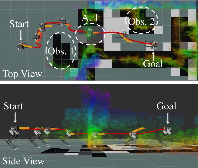
In this paper, we seek to ascertain the feasibility of utilizing a dynamic bipedal walker Cassie to explore and navigate in congested and unknown environments, as shown in Fig. 1. To enable bipedal robots, like Cassie, to navigate autonomously in height-constrained spaces without prior knowledge of the environment, three major problems should be addressed. Firstly, a collision-free path should be found and updated quickly from the current position to the goal location while exploring in the unknown space with varying admissible heights. Next, a local trajectory for the bipedal robot is required with consideration of obstacle avoidance and robot’s physical limitations. Moreover, the planners also need to ensure the gait stability of the underactuated bipedal robot, i.e., the planners should respect the underactuated dynamic coupling and prevent the robot falling and hurting nearby humans and the robot itself. Finally, to enable the robot to reliably follow the planned motions, we need a walking controller that can change the robot’s configuration, e.g., walking height, while maintaining stable walking gaits with different velocities. While these problems are challenging, a solution that addresses them will enable end-to-end navigation for bipedal robots for autonomous and safe travel in unknown height-constrained environments.
I-A Related Work
I-A1 Motion Planning for Legged Robots:
Motion planning for legged robots has been an attractive topic and usually involves planning in the configuration space. In some prior work, paths of the root of robots are firstly found, for example, by sampling-based methods such as RRTs presented in [4, 3, 5, 6]. Later, robot footholds are selected over uneven terrain and the configuration of the whole body is planned by imposing foot contacts and stability constraints, such as [7, 8, 5]. There are other approaches that choose to plan reachable and optimal footholds over terrains first, and then generate the whole body motion using constrained optimization, see [9, 10, 11, 12]. Besides stepping over uneven terrain, some approaches also consider avoiding obstacles in confined spaces as demonstrated in [1, 3, 13], but only simulated results are presented. Recently, a hierarchical motion planning framework and experiments on quadrupedal robots to travel in height-constrained environments is presented in [6]. In this work, a path of robot pose is firstly randomly sampled by RRT-Connect in [14], followed by path smoothing while avoiding collision through CHOMP in [15]. Footholds are selected via the method shown in [7] and posture of the robot is optimized again to adapt to the planned foot placement. However, this last step in the pipeline ignores potential collisions, which prevents the entire framework from making collision-free guarantees.
Moreover, the above-mentioned motion planning work for legged robots only considers planning in configuration space without the dynamics of the legged robot, which results in slow and statically stable gaits. This could also lead to failures in experiments as reported in [6].
I-A2 Trajectory Optimization for Bipedal Robots:
More recently, a kino-dynamics model is leveraged in a Model Predictive Control (MPC) framework to enable a quadrupedal robot to autonomously avoid obstacles in confined spaces including height constraints by [16] using quasi-static gaits. However, collision-free navigation while considering dynamic feasibility for bipedal robots is more challenging. This can be solved by formulating online optimization problems that enforce the bipedal robot’s dynamics constraints. Using full-order dynamic models of high dimensional bipedal robots in online optimization is computationally expensive. A widely-used alternative approach is through simplified models which approximate the walking dynamics, such as the Linear Inverted Pendulum (LIP) models, see [17, 18], and Spring-Loaded Inverted Pendulum (SLIP) models, see [19, 20, 21, 22], based on stability criterion such as Zero Moment Point (ZMP) in [23] or Capturability in [24].
In some approaches, reduced-order models such as centroidal model in [2] or Center-of-Mass (CoM) model in [25] are utilized to optimize for CoM trajectories while enforcing contacts and ZMP constraints, see [26, 27, 28]. Among these, [2] enables person-sized humanoid robots to travel in confined spaces, such as an obstructed door, without collision in simulation. However, in implementations on physical robots, these methods usually limit the robot’s vertical movement, i.e. robot’s walking height is fixed to make the ZMP dynamics linear for online control, such as [29, 18, 30]. Dynamics of LIP without fixed height constraints is studied in [31] where a Variable-Height Inverted Pendulum (VHIP) is proposed to enable walking while changing heights for humanoids based on capturability in simulation. However, the introduction of variable height to the LIP model is more to improve the control performance on the robot rather than to change the robot walking height significantly and enable travelling underneath obstacles.
Cassie, which is more agile with linear feet, cannot use the above-mentioned ZMP-based approaches, see [18]. Trajectory optimization for Cassie is demonstrated in [32] and is formulated using MPC based on SLIP model in simulation. A LIP model based MPC is also developed in [33] for discrete-time safety-critical trajectory generation proposed in [34] for Cassie. But both of them lack experiments on hardware. MPC is also utilized in [35] on a Hybrid LIP (H-LIP) model of Cassie to track a simple global trajectory in experiments and to avoid nearby obstacles in simulation. There is a concurrent work in [36] on building navigation autonomy of Cassie using a RRT as a global planner and a Control-Lyapunov Function (CLF) as a local trajectory planner. But this work doesn’t consider obstacle avoidance during the local planning. Moreover, these works don’t consider the coupled walking dynamics between planar and vertical directions and don’t study autonomous navigation in confined or height-constrained spaces.
Furthermore, almost all prior work on using reduced-order models to generate trajectories for walking robots forces the robot to mimic walking patterns computed by reduced models, like [32, 31, 35]. Such an approach is effective but loses information and properties of the full-order model dynamics of the robots, thus leading to difficulties during experimental implementation on real robots, such as on Cassie as described in [32, 35]. As we will see, we leverage a reduced-order model to capture the control design and its limitation on the full-order model, enabling us to achieve more agile motions during navigation on Cassie.
I-A3 Bipedal Locomotion Control:
Developing a reliable locomotion controller for a bipedal robot to follow the planned footholds and configurations is critical to complete the navigation pipeline. There is a large body of literature to tackle this problem, see [37, 29, 38]. Hybrid Zero Dynamics (HZD) presented in [39] offers a mathematically rigorous procedure to generate stable, fast and energy-efficient periodic gaits using the full robot model based on input-output linearization. Moreover, the stability of gait transition using HZD is studied in [40] and applied to the problem of navigation by transitioning between limit-cycles and validated on bipedal walkers in simulations, such as [41, 42, 43]. In experiments, HZD is validated on a range of bipedal robots with point or linear feet in [44, 45, 46], and more recently, on Cassie in [47, 48, 49]. Based on [47] and HZD, a walking controller that is able to control a bipedal robot to crouch is firstly developed in [48]. Variable walking height control problems are later explored by a reinforcement learning method in [50] and by an H-LIP-based approach in [51]. In this work, we use the HZD-based controller on Cassie constructed by [48].

I-B Contributions
The primary contributions of this work are: (1) the design and development of one of the first autonomous navigation frameworks for underactuated bipedal robots to navigate unknown height-constrained environments. In this framework, search-based A* and collocation on a reduced-order dynamical biped model work as global and local planners, respectively. (2) A vertically-actuated SLIP model (vSLIP) is introduced to describe the coupled walking dynamics for variable walking heights and walking velocity and to reduce the online computation burden. Unlike previous attempts to force physical robots to mimic reduced-order models, we introduce a modelling method in the vSLIP to capture the properties and limitations of HZD-based locomotion control that leverages the full-order dynamics model. (3) Such a reduced-order model is utilized in hierarchical collocation-based trajectory planners to find trajectory profile and real-time control commands that also respect gait stability and safety constraints for bipedal robots. (4) Using the proposed framework, we present experiments on the bipedal robot Cassie illustrating safe navigation in height-constrained environments. This framework is one of the first to demonstrate considerable level of autonomy to enable a bipedal robot to travel without collision nor losing balance while exploring various unknown confined environments. This proposed autonomy serves as a milestone towards real-world deployment of person-sized bipedal robots like Cassie.
I-C Paper Structure
The paper is structured as follow. The overview of the proposed navigation autonomy is introduced in Sec. II. In Sec. III, the Cassie experimental platform is introduced and its HZD-based variable walking height controller is briefly discussed. The gait stability constraint of this walking controller is also introduced there. Sec. IV develops the vSLIP model to capture variable height dynamics and limitations of the HZD-based controller, which is later utilized in optimization-based local trajectory planners developed in Sec. V. Robot localization, mapping, and global planning are presented in Sec. VI. Numerical validation in simulation and experimental results are presented in Sec. VII and Sec. VIII, respectively. The proposed autonomy is also extended to navigating on height-constrained sloped terrain in Sec. IX. Conclusion and future work are discussed in Sec. X.
II Overview of the Navigation Autonomy
The proposed autonomous navigation framework for the Cassie bipedal robot is illustrated in Fig. 2. The core part of this autonomy is the hierarchical design of the planners. This includes a (1) global planner to search for a collision-free path on the global map, (2) a local planner to generate dynamically-feasible trajectory to lead the robot to track a local goal location from the global planner while avoiding nearby obstacles, and (3) a reactive planner outputting real-time commands to the walking controller while providing dynamic feasibility and safety guarantees.
In this framework, the environment is perceived by a RGB-Depth camera, and the detected obstacles are classified as non-traversal areas and height-constrained areas (Sec. VI-B). The detected obstacles are registered into a 2.5D grid map as demonstrated in [52] which encodes the information of admissible walking height in each grid, and the map is updated at 1 Hz. Moreover, the robot’s odometry is estimated simultaneously by a tracking camera based on Visual Inertial Odometry (VIO) as discussed in [53] at 30 Hz.
After being given a goal location, a global planner using A* is designed to find a path of collision-free waypoints on the map from the robot’s current position to the goal (Sec. VI-C). A local goal is found on the global path within a range of the robot’s current position, e.g., a local goal which is 1-meter ahead of the current robot position, to send to the local planner. The global planner and the local goal are updated at 1 Hz in order to synchronize with the local planner.
After being given the position of the local goal from the global planner, an optimization-based local planner (Sec. V-B1) uses vSLIP dynamics to compute a dynamically feasible state profile to reach the local goal. This local planner not only respects the robot’s gait stability constraints but also ensures the robot avoids obstacles. The resulting trajectory from this local planner lasts 3 seconds and is replanned every 1 second in this work. This local planner provides a smooth trajectory to lead the robot to reach the local goal that is 1 meter ahead. However, the 1 Hz frequency of this planner is still not fast enough for an agile dynamic walker when it is exploring an unknown and confined environment. Therefore, a reactive planner (Sec V-B2) that replans at higher frequency, 10 Hz, is developed.
This reactive planner uses the same optimization schematic as the local planner but has a shorter-term preview, replans at 10 Hz and outputs a short-term discrete state profile. Its target state is chosen as 0.3 m ahead of robot’s position in the planned state profile from the local planner. It only sends the walking velocity and walking height from the closest planned state as the real-time command to the walking controller. As we will see, this reactive planning strategy helps ensure that each control command has a guarantee of dynamics feasibility, gait stability, and collision-free safety. Moreover, in this way, we can combine the advantages from the local planner, that is the ability to have longer preview of the robot’s trajectory, and the one from a fast reactive planner that is to handle real-time disturbances and modeling error of the reduced model.
After being given the planned walking velocity and walking height, the variable walking height controller sends torque commands to the robot at 2 kHz. Moreover, the robot states for the controller is estimated quickly based on robot kinematics model using onboard sensors such as motor encoders and IMU. As there is no pre-built map used, this vision-to-torque framework can enable bipedal robots to safely navigate with agility in new unknown cluttered and height-constrained environments without losing balance.
III Cassie and Locomotion Control
Having introduced the overall navigation framework, we next present Cassie and its variable walking height controller to better understand properties of the system to plan for.
III-A Cassie Robot Model

As presented in Fig. 3, Cassie is a dynamic, underactuated legged robot and has 20 DoFs. It has ten actuated motors and four passive joints on its Left/Right legs. Its pelvis, i.e., floating base, has 6 DoFs that represents sagittal, lateral, vertical transitions and roll, pitch, yaw rotations, respectively. The floating-based coordinate captures the joint angles and the pose of the robot. The underactuation in the robot is primarily due to the fact that the feet only have a pitch DOF and can’t roll. Additional underactuated DOFs exist in the form of the two passive springs in each leg. The virtual leg length and leg pitch angle are denoted by and , respectively. Unlike its predecessor robots such as [44, 45], Cassie can not only walk in the saggital direction but can also walk in the lateral direction as well as turn. Such an ability gives it advantages to serve as a robotic platform in navigation tasks. Moreover, we summarize the notations and symbols we frequently use in this paper in Table I.
| Full-Order Model | |
| Floating based coordinates | |
| Base (pelvis) translational coordinates | |
| Base rotational coordinates | |
| Motor positions on Left/Right Leg | |
| Virtual leg length and leg angle | |
| Gait Library | |
| Gait parameter | |
| Periodic gait | |
| Gait library | |
| Variable Walking Height Controller | |
| Commands to the controller | |
| Convex feasible command set | |
| vSLIP Reduced-Order Model | |
| States | |
| Inputs | |
| Foothold position on flat ground () | |
| , | Current and uncompressed leg length |
| Total mass of the robot | |
| Leg stiffness | |
| Trajectory Optimization | |
| Safe set | |
| , | Radii of obstacles and robot footprint |
| Minimum admissible height nearby | |
| Safety margin | |
| Slack variables | |
III-B Gait Library
To obtain dynamically-feasible walking behaviors for the bipedal robot Cassie, we generated a set of periodic walking gaits by formulating a direct-collocation based optimization using the full dynamics model of Cassie with HZD as described in [48, Sec. III] based on [47, 54]. A gait is defined as a periodic state trajectory for all actuated joints. For each gait, represents its gait parameter. Then, a gait library is formulated by indexing each optimized gait with its gait parameter . We generated a gait library offline with 1331 gaits with the gait parameters as described in Table II.
III-C Variable Walking Height Controller
In the real-time controller as shown in Fig. 2, a reference gait is obtained by linearly interpolating the gait library with respect to the observed current robot’s gait parameter . A PD-based gait regulator is deployed to correct the gait in order to track the desired commands . The control command in this work includes desired sagittal walking speed , lateral walking speed , walking height , and turning yaw velocity , i.e., . This is achieved by adding regulating terms to the reference gait and the resulted regulated gait is sent to joint level PD controllers to generate motor torques to control the robot. More details about this controller can be found in [48, Sec. IV] which is extended from [47]. In particular, this controller is able to regulate the robot to the command .
III-D Convex Feasible Command Set
There exists varying velocity upper and lower bounds with respect to the variable walking height controller described, e.g. when robot walks with a low walking height, it can’t walk fast. In order to quantitatively analyze such constraints, a feasible command set is constructed as shown in Fig. 4. This set is obtained in a high-fidelity simulation, MATLAB SimMechanics, with full-order dynamics of the Cassie walking robot.
| number of gaits | |

During each iteration in the simulation, a test command is sent to the tracking controller. If the controller succeeds to maintain a stable walking gait on the robot for 30 seconds, i.e. the robot doesn’t fall, that input command is recorded as a feasible command. Otherwise, that command will be considered as infeasible and not recorded. The testing range for is between and with a resolution of and a finer resolution at the border. We collect all the feasible commands as the yellow circles shown in Fig. 4 and these form a Feasible Command Set.
In this set, the maximum positive sagittal walking velocity grows as the walking height increases, after reaching its maximum around m/s, at around m, it drops dramatically. The maximum negative and lateral walking velocity have similar trends but they reach their maximums, m/s and m/s, respectively, at m. Note that the backward walking behavior in the feasible set is not symmetric to the forward walking one while side walking behavior is symmetric about the plane. Moreover, the feasible walking height command range is m. The range of feasible turning yaw velocity command is not dependent on other dimensions, therefore, for simplicity, it is not visualized in Fig. 4, and the range is deg/s.
Furthermore, several feasible points are selected as vertices, which are represented by solid red points in Fig. 4 to form a conservative convex subset of the original feasible command set. This is defined as Convex Feasible Command Set , and its vertices are . As long as a given command is within this convex feasible command set, the resulting closed-loop gait obtained by the controller enforces gait stability (in the sense of not falling) on the full-order model. As we will see, the convex feasible command set will enable us to plan using the reduced-order model while still ensuring stability on the full-order model.
Since the HZD-based walking controller used in this work realizes periodic walking gaits, the feasible command set numerically captures the stability of the resulting periodic motions using the closed-loop controller for each command on the 3D bipedal robots. Since the walking period is second in this work and simulation time is relatively long ( sec) which results in roughly full-cycle walking, the resulting motion has already become periodic if it is stable, and the robot will not fail to keep this gait during a longer test time in the absence of external perturbation.
The concept of a feasible command set was initially introduced in [50] to quantitatively compare the ability of different controllers on bipedal robots. However, using the convex subset to ensure the gait stability of the command input is first introduced here.
IV Vertically-actuated Spring-Loaded Inverted Pendulum (vSLIP)
In this section, we develop a reduced-order model we call vertically-actuated Spring Loaded Inverted Pendulum (vSLIP) to approximate the walking dynamics in planar and vertical direction for bipedal walking robots. Compared to previous reduced-order models, such as SLIP, vSLIP introduces one more actuation in the vertical direction. Moreover, the modeling of vSLIP considers the design and limitation of the robot controlled by a HZD-based controller in order to bridge the full-order model and the reduced-order model.
IV-A Bridging the reduced-order model and full-order model
Prior approaches first design reduced-order models and later develop controllers to force the robot to mimic the motions obtained from the reduced-order model such as [32, 31, 35]. Our approach differs from this and first develops a library of dynamically feasible periodic gaits on the full-order model along with a variable walking height controller that stabilizes to a chosen periodic gait on the robot. As illustrated in Fig. 5, we consider and utilize the restrictions coming from the full-order dynamics, the controller, and the robot in the reduced-order model. In this way, we enable the online generation of motion plans on the reduced-order model that will be feasible on the full-order model. Specifically, this is achieved in a threefold manner: (i) We extract the foot placements from the periodic orbits in the gait library that are optimized with the full-order model; (ii) We use the convex feasible command set describing the feasible commands to the controller, and this represents restrictions on walking velocity and walking height that result in stable gaits; (iii) We measure physical parameters of the robot. These are then used in the reduced-order model, vSLIP, so that this model captures the information and limitations of the full-order dynamics, the controller, and the physical robot.

IV-B Model Representation
The mathematical representation of vSLIP model is described in detail in this section. In vSLIP, the bipedal walking robot is simplified as a point mass supported by a massless leg with a spring and actuators during one walking step. When one step ends and another step begins, i.e., transition happens, the stance leg spontaneously switches. The state represents the Cartesian 3D position and velocity of the Center-of-Mass (CoM), and turning yaw and turning velocity of vSLIP. The dynamics could be defined as , presented as follows:
| (1) |
where is the virtual input acting on the CoM and . Here, is the total mass, and are the leg length and uncompressed leg length of the reduced-order model, respectively, and is the stiffness of the leg. Moreover, the values of , and are measured from the robot. Note that the leg stiffness parameterized as a function of the leg length is defined as below (see [55] for more details),
| (2) | ||||
| (3) |
In the vSLIP model, the walking dynamics of planar motion (xy-plane) and vertical motion are coupled by virtual leg length. Moreover, vSLIP has one more actuation in the vertical direction compared to previous SLIP models in order to change the virtual leg length significantly. Furthermore, we decouple turning dynamics from other dimensions and simply model it as a double-integrator system.
Remark 1
The way that we model the turning yaw dynamics is inspired by previous HZD-based locomotion controls in simulation and experiments where yaw doesn’t affect motions in other dimensions significantly. But it does have constraint on turning velocity, i.e., the robot cannot change its heading orientation too fast.
In (1), the foothold position is defined which represents the step length and step width of vSLIP on flat ground () between two adjacent walking phases. The foothold for the next step is obtained at the end of each step. For brevity, the superscript prime indicates the next step. To plan for trajectories for walking robots, the foothold position is usually required to be jointly planned with model state as in prior work, see [6, 27]. Moreover, there exists constraints on step length and step width to make the planned foothold reachable, e.g., the leg cannot extend too long. This actually brings challenges to quickly solve the planning problem. In the following part, we introduce the foot placement heuristics coming from the HZD-based gait library that can be utilized in vSLIP for online computation.
IV-C Foot placement heuristics
In this part, we take advantage of the fact that the foothold planning and constraints are already considered during full-order model based gait optimization, and use the resulting foot placement into the reduced-order model vSLIP. In Sec. III-B, the precomputed gait library optimized by the model of the robot already contains the foothold position for different gait parameters. The optimized foothold position represents the limitations on the robot’s strides since the robot dynamics and physical constraints are considered during optimization. Therefore, taking advantage of the HZD-based gait library, in this work, foothold position of vSLIP doesn’t need to be planned online. More specifically, the information of step length and step width is decoded from the optimized library and is utilized into the reduced-order model dynamics to fasten computational speed while ensuring the planned foothold to be reachable. Interestingly, through our study, the foot placement for next step is a function of the gait parameters at the end of step, i.e., during transition between adjacent gaits. We denote this function as foot placement heuristics, and it can be calculated via:
| (4) |
where is the state of the end of one step, and , , are the leg length, leg pitch, and abduction, at the beginning of next gait.


They can be formulated as explicit functions of the state of the end of one step, as shown in Fig. 6, and the data points are obtained from the gait library with different gait parameters. To alleviate the complexity, we choose a first-order polynomial model to fit those data. This fitting could be described as:
| (5) |
where and are the coefficients that could be solved with linear regression. In this way, the foothold values can be updated by the gait parameters at the end of each step, presented in (4) and (5).
In conclusion, we describe the reduced vSLIP model in a manner of using the information and limitations from optimized gait library, walking controller, and physical robot based on full dynamics model. In return, this reduced model can be used online to generate dynamically-feasible reduced-dimensional state profile for the actual closed-loop system which is the robot controlled by a walking controller.
V Optimization-Based Trajectory Planners
The goal of this section is to use the vSLIP model to formulate a nonlinear program to optimize for dynamically-feasible trajectories to drive the robot to track the given local goal while respecting various constraints. We first introduce the formulation of collocation-based trajectory optimization on vSLIP to reach a target state. As mentioned in Sec. II, such a formulation is used in both a local planner and a reactive planner. After presenting the trajectory optimization problem, we also discuss and compare the local and reactive planners.
V-A Trajectory Optimization


V-A1 Formulation
The trajectory optimization is applied on vSLIP and is formulated using a collocation method. States and inputs are defined in the vSLIP model in Sec. IV. The nonlinear optimization problem is on discrete collocation nodes with time step and fixed time span .
Given initial and target state as and , the collocation optimization could be formulated as follows,
| (6a) | ||||
| s.t. | (6b) | |||
| (6c) | ||||
| (6d) | ||||
| (6e) | ||||
| (6f) | ||||
| (6g) | ||||
| (6h) | ||||
| (6i) | ||||
where the cost function is designed as below,
| (7) |
where , and , and they are diagonal matrices with non-negative entries. Specifically, is the weight for state cost and has positive values on the velocity terms and zero for the position ones. Smoothing cost weight is introduced to smooth the trajectory, and input cost weight penalizes the virtual input representing the acceleration terms of the vSLIP. Furthermore, admissible state set and input set , safe set , admissible height and its safety margin , initial condition and target state will be explained in the following section.
The time span for this optimization could cover multiple walking steps which are described in Sec. IV-B. At the end of each step, the foothold in the next step will be updated by the foot placement heuristics (4).
Moreover, is defined as . This represent a vector of slack variables used in the constraints, and diagonal matrix has all positive entries and is sufficiently large to minimize the slack.
V-A2 Constraints
The constraints that the optimization problem (6) enforces during the navigation in height-constrained environments mainly contains the state and input bounds, initial and final state conditions, dynamic feasibility, avoidance for both ground obstacles and overhanging obstacles, and gait stability of the robot. These can be summarized as follows.
Dynamic feasibility
Leg length
States bounds and gait stability
The admissible state set in (6d) is the intersection of two sets: states within upper and lower bounds and states within the convex feasible command set introduced in Sec. III-D. The admissible state set is
| (8) |
Since is a convex set, it can be described by its vertices (Fig. 4) such that
| (9) |
The above constraint at the node can then be rewritten as follows,
| (10a) | ||||
| (10b) | ||||
| (10c) | ||||
where are Lagrangian multipliers. If the optimizing states meet (10), the walking controller will be able to maintain a stable walking gait on the robot since the command is feasible for the controller as illustrated in Sec. III-D. A slack variable vector is added to allow small violations to ensure the feasibility of the optimization problem.
Collision-free safety
The robot should be able to avoid obstacles along the trajectory and this is achieved by limiting all states in the safe set of node in (6e), as illustrated in Fig. 7(a). This safe set is formulated as follows,
| (11) | ||||
where represents planar position of the detected obstacle and encodes that obstacle’s size. stands for the robot shape. In this case, it is set to m which is Cassie’s footprint size. norm is used to better describe the shape of rectangle obstacles. The constant is set to be a safety margin for obstacle avoidance. Another vector of slack variable is included to attain the feasibility of the optimization problem. However, this slack variable should be always larger or equal to zero to avoid collision.
Admissible height
In the environment with varying height constraints, there may exist different admissible heights in the robot surrounding, as shown in Fig. 7(b). Therefore, a conservative way to apply the height constraint is to set the height of the robot in the last half of the trajectory to be less than the minimal admissible height in the local region as given by (6f). Moreover, a safety margin of the robot height is included. Enforcing this constraint in the last half of the trajectory could guide the robot to lower its height early to have a smooth height transition and to prevent the robot crouching down too slow to avoid colliding with the ceiling obstacles.
Initial and final states
The starting node should be equal to the current observed robot state , enforced by (6g). Similarly, the terminal node should also stay close to the given target state , enforced by (6h). But the target state may not satisfy other constraints, e.g., the target state is very close to the obstacles or is unreachable for the robot dynamics in the given time span. Therefore, a vector of slack variable is added to adjust the distance between and to ensure the feasibility of the optimization.
Input bounds
Equation (6g) restricts the virtual input to stay in the admissible input set . This could help to bound the acceleration along the trajectory, which could also smooth the optimized trajectory as contains acceleration of the vSLIP. Please note that the inputs are virtual and represent acceleration terms of the vSLIP model in (1). The actual commands given to the locomotion controller are functions of the states . The input bounds here are redundant terms and can be a very large range. These are to prevent unbounded acceleration in the optimized state trajectory if the stage costs are all zeros ().
V-B Local planner and reactive planner
As explained in Sec. II, the local planner and reactive planner share the same optimization schematic explained above but serve different proposes: the local planner has longer preview to generate a smooth trajectory to lead the robot to reach the local goal location, while the reactive planner has a shorter preview but replans in a high frequency to obtain real-time commands for the controller. The output from the local planner is marked as the yellow trajectory in Fig. 7 and the plan from the reactive planner is shown as the blue trajectory in Fig. 7. The comparison between these two planners is illustrated in Table III and is explained in detail as follows.
| Local Planner | Reactive Planner | |
| Num. of steps | ||
| Time span | s | s |
| Horizon | ||
| Apply (6f) | Yes | No |
| Target State |
V-B1 Local Planner
The role of the local planner is to generate a smooth local trajectory which complies to constraints to lead the robot to the given local goal that is 1 meter ahead. As shown in Table III, this planner uses a preview with walking steps elapsing 3 seconds, and replans around every 1 second. Such long-term preview brings benefits to the robot with longer prediction and therefore enables the robot to proceed to avoid obstacles and change walking height early with a larger safety margin. For example, as illustrated in Fig. 7, the height constraint (6f) is enforced on the last half of the planned local trajectory. This prevents the robot from being too late to crouch down and to avoid the height constraint. The target state is set to , as marked as dark yellow in Fig. 7(a), where the desired position terms is the given local goal location, and the velocity term is zero. The given local goal is selected as one-meter ahead of the robot’s current position, and is found on the global path. Moreover is set to 1 m to encourage the robot to recover to normal walking height (1 m) if possible. As this 3-second local trajectory will be updated every 1 second, robot will only follow less than half of the trajectory. The second half of the local trajectory with zero terminal velocities serves as a backup plan to decelerate the robot and step in place in case of a planning failure.
However, this planner suffers from a drawback. The robot may deviate from the planned trajectory during the 1-second update due to tracking errors of the controller or due to environmental perturbations. Especially, it is risky to allow person-sized bipedal robots to follow a path without any feedback and correction for 1 second. Therefore, a reactive planner running at a higher frequency is needed.
V-B2 Reactive Planner
The reactive planner is designed to run at 10 Hz in real time to enable the robot to track the planned local trajectory. The fast computational speed is achieved by only planning for a single step with a horizon length of 6. Besides the horizon difference, the reactive planner has several variances from the local planner. Firstly, as the planned reactive trajectory is short, satisfying the height constraints for half of the horizon may not be feasible. Therefore, as mentioned in Table III, (6f) is not enforced in this planner. Secondly, the target state for the reactive planner is chosen from the local trajectory with a range of m, and not only includes target position but planned velocity, as shown in Fig. 7(a). Apart from these two changes, the reactive planner shares the same constraints and costs as the local planner, ensuring the reactive plan to meet all the constraints. The output from the local planner is a trajectory with 6 nodes, but it only passes the next state to the controller as command where the subscript 1 represents the first node after the initial node 0.
V-B3 Initial Condition
If the initial condition is set to the observed current robot state , the reactive planner is a nonlinear model predictive controller (NMPC). However, due to several factors such as the vSLIP only approximates the robot dynamics and the measured velocities are very noisy on the walking robot, NMPC doesn’t work well in the experiments on Cassie. Therefore, the initial condition is set to a combination of feedback and feedforward terms: the position part except in the is measured while the rest is the last timestep output from the reactive planner, and the local and reactive planners share a same initial condition.
V-B4 Solving the Optimization
The optimization problems for the long-term planner and reactive planner are formulated using CasADi in [56] and solved by IPOPT in [57] with the initial guess linearly interpolated between the given initial condition and target state .
In this manner, we obtain the major part of the proposed autonomy which is the pipeline to go from a given local goal to real-time control commands for walking robots. This is realized by using the cascading trajectory planners to optimize for a local plan with long preview and a reactive plan with fast replanning. The trajectory optimization schematic used in these two planners leverages vSLIP to ensure dynamic feasibility, collision-free safety, and gait stability for bipedal robots, and can be utilized online.
VI Localization, Mapping & Global Planner
After the development of trajectory planners for Cassie, the infrastructure of the navigation autonomy, such as perception and localization of the robot, world representation via a 2.5D map, and the global planner to provide a path to reach the given goal, is introduced in this section.
VI-A Perception and Localization
Cassie’s perception is based on robot vision, and it is equipped with one tracking camera (Intel RealSense T265) and one RGB-Depth camera (Intel RealSense D435i). Both of them are fixed on the top of Cassie’s pelvis, as shown in Fig. 3. The tracking camera is able to estimate the odometry of the robot’s floating base which is by Visual Inertial Odometry (VIO) demonstrated in [53] at 30 Hz. The RGB-Depth camera is utilized to perceive the robot’s surroundings by filtered pointclouds and runs at 30 Hz.
VI-B Mapping
A RTAB-Map presented in [58] is used in real time to localize the perceived historical pointclouds in the map by optimizing over the 3D map’s graph with proximity detection and estimated robot odometry, see [59]. The RTAB-Map updates at 1 Hz and the resolution of the voxels is 0.1 m in 3D space. In this way, the perceived 3D environment can be described by an Octomap in [60] as shown in Fig. 8. With an assumption that the robot walks on a flat ground, the obstacles on the ground can be extracted by removing the voxels that are lower than a given threshold.
VI-B1 Global Map
In order to utilize the spatial information for spontaneous planning, the 3D map is later translated to a 2.5D map where the minimum height of the voxels on the Octomap is recorded on the corresponding 2D cell on the grid, as exemplified in Fig. 8. The minimum height of the voxels over the ground at the same 2D position is termed as admissible height to the robot, because it describes the maximal walking height on that 2D cell.
Remark 2
The sensor stack on top of Cassie adds a 0.25 m vertical dimension to the pelvis height , as shown in Fig. 3. In this work, admissible height refers to the maximum walking height and ceiling height includes this 0.25 m vertical dimension.
Compared to Octomap, the 2.5D map has a size of 20 and has a lower resolution of 0.5 m. The admissible height recorded in this map is obtained by finding the lowest height of the 0.1 m resolution voxels inside the low-resolution cell, as shown in Fig. 8. Such low resolution grid is able to take the robot shape into account because Cassie’s footprint radius is around 0.2 m. In this way, each cell on this 2.5D map can be classified into four types of space for the robot with respect to its admissible height:
Obstacle
The admissible height is lower than the robot’s lowest walking height (0.7 m) and is, therefore, not traversable for the robot.
Height-constrained
The admissible height is within the robot’s lowest and largest walking height (1 m) because such a region is traversable but requires the robot to lower its walking height to be below this admissible height.
Free
The robot can travel through it using its largest walking height.
Unexplored
The low-resolution cell that has not been well perceived and does not have obstacles, i.e., only part of this cell is detected as free space.


In this way, planners can utilize the information on this 2.5D map to find an optimal path to navigate the robot while considering the varying admissible height and obstacles in the environment. The global planner is deployed on this 2.5D global map while trajectory planners developed in Sec. V only use the information of a small region on the global map which are denoted as a local map.
VI-B2 Local Map
For optimization-based trajectory planners that only plan for short trajectories, the information over the entire map is not necessary. Therefore, a local map that only contains the environment information of the robot’s surroundings is built. In this work, the local map is designed to be a bounding box whose width is 1.2 m and length is 2.75 m, and is shown in Fig. 8 as the pink bounding box. The location and orientation of this local region can be well defined by the robot’s current position and the local goal for the local planner and can be updated in real time. The locations of all the obstacles, i.e., 0.5 m untraversable cells, inside this local map will be considered in the collision-free constraints via (6e) in Sec. V, which are termed as local obstacles in Fig. 8. The minimum admissible height in this region will be added to the height constraint by (6f).
VI-C Global Planner
VI-C1 A* Search
In the scenario where the robot is exploring an unknown environment, a global planner is needed to quickly find a collision-free path (a list of waypoints) to lead the robot to reach the goal location on the global map and should be able to replan when the map is updated. Moreover, in the height-constrained environment, we prefer the robot to avoid traveling underneath obstacles if the robot can walk around the obstacles. Therefore, an A* search presented in [61] that encodes the costs of different types of regions on the map is introduced to serve as the global planner. The cost of each node , i.e., traversal cell, during the search is defined as where is the cost of coming from the start node to the current node while is the heuristic cost that is defined as
| (12) |
where is the Euclidean distance to the goal location and is the cost of admissible height of the node, i.e., a node that has lower admissible height will have a larger . In this way, the A* will prefer to include the node which has a larger admissible height into the path. Moreover, a node that has not been explored will be avoided if there is a well-known node around, and this is achieved by having a larger weight on the node that is unexplored. In this way, the A* search is able to find an optimal path that is shortest to the goal location while avoiding height-constrained and unexplored regions if possible.
VI-C2 Local goal
This global planner returns a sequence of waypoints which are the 2D coordinates of the selected nodes in the planned path and these are updated at 1 Hz. The local goal that is ahead of the robot’s current position in a given range will be selected from this global path by a breadth-first search, as marked in Fig. 8. In this work, the local goal is chosen as 1-meter ahead of the current estimated robot position. Specifically, the nearest two waypoints around one-meter ahead are found first and then a linear interpolation between these two waypoints allows us to select the local goal. This local goal selected by the proposed approach is continuous with respect to the robot’s movement and is passed to the local planner as part of the target state via (6h) in Sec. V.
By now, the infrastructure for the autonomy is developed, and the trajectory planners and walking controller can be embedded in this framework to drive the bipedal robot to safely explore height-constrained environments as illustrated in Fig. 2. The entire pipeline is validated next in simulations and experiments in the following sections.
VII Numerical Validation
In order to validate the proposed navigation framework and exemplify the necessity of the feasible command set introduced in Sec. III-D and used in Sec. V, the proposed navigation autonomy is deployed on the bipedal robot Cassie and is tested extensively in a joint Simulink-Gazebo simulation for simulating dynamics and vision.
VII-A Simulation Implementation
We utilize Gazebo to simulate the robot’s depth camera reading and MATLAB Simulink to calculate the robot full-order dynamics in order to have a higher fidelity simulation of the robot’s walking dynamics. These two simulators are synchronized and the navigation algorithms are running online during simulation. Specifically, the simulation of robot dynamics and vision will not wait for the results of planners and the controller, which is aligned with the real-world setting. The planning data is visualized via ROS RViz, as shown in Fig. 9(a),9(c).
For the simulation test, a congested space with an arch whose admissible height is 0.75m and two obstacles are constructed in Gazebo, as demonstrated in Fig. 9. The initial position of the robot is behind the first obstacle and the goal location is set to be close to the second obstacle.
VII-B Validation of the Proposed Autonomy
The proposed navigation pipeline shown in Fig. 2 is first tested in the simulation. It demonstrates the capacity to drive the robot to avoid the first obstacle, crouch down to pass through the arch, recover to a normal walking height afterward, and then stop in front of the second obstacle. All this is done without a single fall or collision, as exhibited in Fig. 9(a). The profiles of the robot’s planned and actual walking speeds and walking height are recorded in Fig. 9(b).
VII-C Autonomy without Feasible Command Set
In order to demonstrate the necessity of the feasible command set during the navigation, we consider the pipeline as introduced in Sec. V but remove the feasible command set which introduces a gait stability constraint via (10). This is compared with the original pipeline without changes. The parameters used in the walking controller, cost functions (7), and the rest of the constraints in Sec. V-A2 are kept identical to obtain a fair comparison.
As shown in Fig. 9(c), the navigation autonomy without the feasible set causes the robot to fall. This occurs when the robot is approaching the goal location while increasing the walking height after the robot walks through the arch and avoids collision with the second obstacle.
According to the recorded data in Fig. 9(d), during the period of 28 s to 30 s, when the robot is changing its walking height from 0.75 m to 1 m while walking to the left, the profile of planned walking height is much steeper than the one using (10) (28.5 s to 32 s in Fig. 9(b)). Because of the coupled dynamics between planar walking velocity and walking height, such fast changes in the walking height triggers a larger robot lateral walking speed under similar planar walking velocity commands. As a result, the robot’s actual lateral speed accelerates to over 0.4 m/s during 33 s to 35 s, and the planner needs to use a large lateral speed command later during 36 s to 40 s to drive the robot back. At this period, the lateral walking speed command is over -0.2 m/s at of 1 m which lies outside of the feasible command set in Fig. 4, and directly results in gait instability.
This showcases the importance of the feasible command set. Without it, the planned trajectory is not dynamically feasible in the sense that the plan does not take into account dynamic coupling that exists between the planar velocity and the walking height, leading to unbounded robot states and eventually a walking failure like Fig. 9(c),9(d).
We repeated such ablation test at least 5 times with different robot initial states in this simulation and results are consistent across all trials. More extensive tests on the proposed autonomy are conducted in the experiments on the real robot Cassie in the following section.
VIII Experiments


VIII-A Hardware Implementation
Cassie has a real-time computer running the variable walking height controller and kinematics-based state estimation at 2 kHz. There are two Intel NUC mini computers with i7 processors used for the entire navigation pipeline. One computer processes the perceived spatial information and registers it into the 2.5D map. It also communicates with the Cassie’s computer in order to send real-time commands to the controller while processing robot’s state feedback. Another mini computer receives the maps and deals with all planning-related work, data visualization, and provides the planned control commands. The testing cases are indoor scenarios where obstacles are represented by cardboard boxes. Note that while there are some QR codes used in the environments, like the ones in Fig. 10(a), these are only used to add more features to a relative-plain background to enhance the performance of VIO and are not exploited to store prior information of ground truth locations in the environment.
VIII-B Experiments
In this work, the autonomy is tested in four types of indoor environments which include (1) a maze without height constraints, (2) a cluttered space with multiple obstacles and one height-constrained space in the form of an arch, (3) an area that has multiple arches and a ground obstacle, and (4) an obstructed door. The motivation of this study is to validate the proposed legged navigation autonomy that can handle unknown environments with a range of obstacles. Each experiment is designed to test a specific aspect of the algorithm’s performance and build upon the previous experiment.
The proposed autonomy is tested successfully in at least 4 trials where the robot is able to safely walk to the given goal location without a single fall in each of these scenarios. Representative experiments (video111https://youtu.be/Da0tebC3WuE) are exemplified and analyzed below.
VIII-B1 2D Maze
In this scenario, three obstacles are distributed in a cluttered space with 4 m width and 10 m length without any height constraints, as shown in Fig. 10(a). Each of the obstacles is in the shape of 0.5 m1.0 m and they form a maze for the robot. In order to test the ability of the autonomy to explore an unknown and complex environment, Cassie is initialized in front of the first obstacle which blocks most of the view of the robot and therefore the robot has a limited prior information about the entire maze. During the test, as illustrated in Fig. 10(a),10(b), the global planner is able to quickly reroute and create an updated path to avoid the new detected obstacle, while the local planners update in real-time to regulate the robot movement to avoid collision. Moreover, several decelerating maneuvers take place when the robot walks close to the obstacles to ensure the robot’s safety. This is realized by outputting a negative walking speed from the reactive local planner as presented in Fig. 10(c). Between 58 s to 69 s, Cassie enters a very narrow space whose size is only 0.5 m0.5 m, a similar size as the robot footprint, as marked in Fig. 10(b). At this time, the planners slowly change the robot’s movement using almost zero velocity commands, as shown in Fig. 10(c), in order to keep the robot safe. After the robot moves to a more open space, the planners quickly find a trajectory to lead the robot to get out of the current narrow space, which happens after 69 s in Fig. 10(c). As this environment doesn’t have any height constraints, the robot maintains a normal height of around 1 m all the time, as exhibited in Fig. 10(d). This experiment demonstrates the capability of the proposed autonomy of a large-scale humanoid robot to safely navigate in a tight space that has almost the same width as the robot’s footprint.


VIII-B2 Height-Constrained Space
In this test, there is an arch-shaped obstacle with a height of 1 m, causing 0.75 m admissible height, along with two obstacles pinned on the ground. This is shown in Fig. 11(a). The robot is initialized right behind the first obstacle in order to have a limited view of the entire map, and the goal is set to be 8 m ahead of the robot’s start location, as illustrated in Fig. 11(b). After Cassie avoided the first obstacle and saw the overhanging arch obstacle and detected that the admissible height in this area is about 0.75 m, it starts to crouch down to use a walking height of 0.7 m to avoid collision with the ceiling, as illustrated in Fig. 11(d). Later, Cassie starts to enlarge to its normal walking height to 1 m after it passed through this arch. In the meantime, the second obstacle appears in the view of the robot and accordingly, Cassie starts to walk to its right to avoid it and reach its goal location, as shown in Fig. 11(c). Humanoid robots walking underneath similar scenarios are mostly presented in simulation in prior efforts such as [1, 2, 3], which use offline optimization with perfect knowledge of the environment and robot dynamics. This is one of the first experimental demonstrations of a person-sized bipedal robot safely navigating in a cluttered environment that has an overhanging obstacle through real-time online planning.


VIII-B3 Multiple Arches
In order to show the autonomy framework is capable to operate in more constrained environments where the robot needs to keep a low walking height, two arches are placed in the two ends of the 4 m10 m space, respectively, representing the entrance and exit of this constrained area, as demonstrated in Fig. 12(a). Moreover, a 0.5 m0.5 m obstacle is placed inside of this region. In the experiments, Cassie changes its walking height to 0.7 m in order to walk through the first arch, starting after 11 s as shown in Fig. 12(d). During the robot’s travel inside this tight space using a 0.7 m walking height illustrated in Fig. 12(b), there are several deceleration happening in order to finely regulate Cassie’s position to avoid collision with the walls and obstacles nearby, such as 26 s, 38 s, and 42 s in Fig. 12(c). Since there are no more overhanging obstacles detected, the planners start trying to recover Cassie’s height to a normal height, as shown between 21 s to 27 s in Fig. 12(d). However, at that time, the robot has traveled forward and detected the second arch, therefore, the planners quickly replan to keep the robot at a low walking height. After the robot exited this area after 50 s, the robot recovers to a normal walking height. However, as shown in Fig. 12(b) and attached video, Cassie passed the goal location while it is enlarging the walking height. The planner is then able to correct the robot back to the goal location by sending backwards velocity commands as recorded after 65 s in Fig. 12(c). This experiment first exhibits a capability of the proposed autonomy for bipedal robots to keep low walking height under multiple height-constrained spaces while reactively avoiding obstacles.
VIII-B4 Obstructed Door
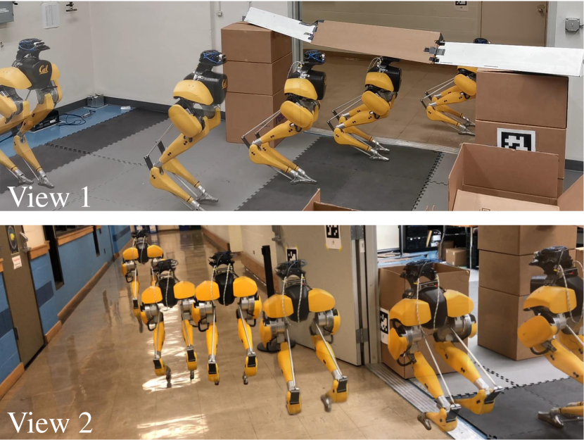
As demonstrated in Fig. 13(a), this environment consists of two parts: a lab space that has a size of 4 m10 m and a corridor that is outside of the lab and has a width of 4 m. There is a door left open connecting these two space and an arch-like obstacle is placed in front of the door. Such an overhanging obstacle adds height constraint to the doorway. The robot is initialized inside the lab and the goal location is set to be outside the lab, as shown in Fig. 13(b). After the robot detected the obstacles and the doorway, the planners start to drive Cassie to its left in order to move towards the target, as shown in Fig. 13(c). In the meantime, Cassie starts to crouch down to avoid the arch obstacle over the doorway. After Cassie moved outside of the lab, obstacles in the corridor, such as the stanchion and the opened door shown in Fig. 13(a) (View 2), can be detected and robot therefore changes its previous plan and keeps moving to its left to avoid these new-detected obstacles. Moreover, when the robot is moving across the doorway, the detected height-constrained grids surrounding the robot are included in the local map, even though the robot is not walking exactly underneath them. Therefore, as illustrated in Fig. 13(d), Cassie keeps a low walking height between 15 s and 30 s in this cluttered environment until 30 s when it travels to an open space and recovers to a normal height. This shows a successful demonstration of a large-scale humanoid robot walking underneath an obstructed door and traveling between different rooms.
IX Extension to Navigation on Height-Constrained Sloped Terrain
While all earlier results are conducted on flat ground, in this section, we extend the proposed method to complex terrains with varying slopes.
In order to realize bipedal navigation on sloped grounds, we require only a few modifications to the navigation framework described in Fig. 2. They are: (i) pre-computing the convex feasible command set on different slopes in the same way described in Sec. III-D, (ii) considering the feasible command sets (by changing the set used in (9)) based on the current slope angle during planning, and (iii) compensating the terrain heights for the detection of the ground and overhanging obstacles during mapping described in Sec. VI-B. We use the same HZD-based variable walking height controller introduced in Sec. III-C as it is robust to the change of ground slope angle in a given range without further tuning or modifications. The controller does not require terrain information.
Followed by the same method introduced in Sec. III-D, we obtained the feasible command sets and their convex subset for the Cassie driven by its variable walking height controller on an inclined slope whose angle is and on a declined slope with an angle of . They are shown in Fig. 14(a). Compared to the feasible command set on the flat ground (zero slope angle) in Fig. 4, we can clearly observe the set shape and volume changes significantly with the change of the slope angles. For example, the feasible command set on the inclined slope shrinks in the backward sagittal velocity dimension while the set on the declined slope is smaller in the lower walking height dimension . This shows that the capacity of the walking controller varies with the changing slope angles and considering such a change during planning is necessary. Therefore, the convex feasible command set used in (9) is updated when solving (6a) based on the slope angle at the robot’s current footprint.
To evaluate the modified navigation framework, we build up a simulation environment where the slope angle of the terrain is varying, as shown in Fig. 14(b). The terrain has a 4-meter-long inclined slope with an angle of , followed by a 2-meter flat ground, and a 4-meter-long declined slope (slope angle is ). There is an arch on each inclined slope and declined slopes and a ground obstacle on the flat plateau. The simulation environment is built in the same high-fidelity Simulink-Gazebo joint simulation of Cassie described in Sec. VII-A.
As demonstrated in Fig. 14(b),14(c), the proposed navigation framework enables the bipedal robot Cassie to navigate on both inclined and declined slopes while avoiding obstacles and changing the walking height to walk through arches without losing balance or collision. In order to reach the target that is set to m ahead of the robot, the robot starts to accelerate after it is initialized on the flat ground. After it walks on the inclined slope, it encounters a height-constrained space, and the robot quickly crouches down and maneuvers through the arch while climbing the slope. After passing the arch, the robot reaches the flat plateau and detected a new ground obstacle. The planner exerts an emerging stop command in front of this obstacle, as recorded around 20 s in Fig. 14(c), and the robot takes side steps to move around it. Afterward, the robot walks to the declined slope and successfully reacts to the newly-detected height-constrained space. The robot reaches the goal location and gets back to the normal walking height after passing this declined slope with the overhanging obstacle.
A limitation of the current method is that the terrain slopes are assumed to be perfectly known and extracting both overhanging obstacles and terrain height on a long slope could be challenging onboard. This drawback from our current robot vision algorithm stops us from deploying the system in the real world. Additional efforts on terrain perception by fusing the IMU reading, the robot’s leg kinematics, and vision, or a better sensor such as long-range 3D LiDAR, can facilitate the real-world deployment of this navigation autonomy.
For other types of rough terrain such as stairs, we hypothesize that the proposed method could also be flexible for the following reasons. On the discrete terrain, the feasible command set can now be formulated to capture the coupled walking dynamics in step length, step width, and step height dimensions, and the rest of the framework can be used. But this may require the development of a precise foot placement controller for a 3D bipedal robot extended from the work like [62], which is challenging.
X Conclusion and Future Work
We have presented one of the first autonomous navigation frameworks for person-size bipedal robots to travel and explore unknown height-constrained and cluttered environments while maintaining gait stability and safety. The autonomy framework is deployed and validated on an underactuated bipedal robot Cassie to travel in various kinds of congested environments. This autonomy leverages a lightweight perception system that only includes an RGB-Depth camera and a tracking camera to perceive the world, along with hierarchical real-time planners.
A global planner using A* search is able to find and reroute the path from the robot’s current position to the goal location while considering the cost of different types of areas while exploring an unknown environment. In order to find a dynamically feasible trajectory for the bipedal robot to track the local goal from the global planner, two optimization-based trajectory planners that consider the robot’s physical limitation, gait stability, and obstacle avoidance are developed for real-time replanning. In this trajectory planning schematic, a local planner schedules a trajectory to reach the given local goal and a reactive planner considers the real-time commands for the variable walking height controller to follow the planned trajectory.
Moreover, a vertical-actuated Spring-Loaded Inverted Pendulum (vSLIP) is developed to capture the coupled walking dynamics of the bipedal robot in the varying walking heights scenarios during trajectory optimization. We introduce a new and practical method to develop and utilize a reduced model (i.e., vSLIP) by first investigating the walking patterns and restrictions on the robot controlled by an HZD-based walking controller, and later utilizing such information in the reduced model for online optimization.
Empowered by the proposed autonomous navigation framework, we demonstrate several successful experiments of Cassie autonomously exploring a diverse repertoire of height-constrained narrow environments, such as a cluttered space with an overhanging obstacle, a region that has multiple arches, and an obstructed door. During the experiments, Cassie exemplifies its capacity to reactively avoid obstacles on the ground and to crouch down and travel underneath arches. Such skills were only realized in simulation with the motions pre-computed offline in most previous work for humanoid robots. Besides allowing the robot to crouch under a minimum ceiling height of 1.0 m overhanging obstacle, the proposed walking autonomy also exhibits the ability to safely walk through a narrow space that is as wide as the robot’s footprint, such as the experiment in the 2D maze. Using the proposed vSLIP model and cascading planning strategy, Cassie never loses its gait stability, i.e., never falls over, throughout the tests of this work.
We next outline a few directions for future work. In our work, we use a single RGB-Depth camera for obstacle detection, enabling the robot to have a small-sized sensor stack and thus enabling walking underneath low-hanging obstacles. However, the field of view of a single depth camera is limited, and therefore, the robot cannot take a wider range of environments into consideration, such as the obstacles behind the robot. This can be solved by upgrading to a 3D LiDAR and this is one of our future work. Moreover, the variable walking height controller used in this work shows some delays and tracking errors not only in the walking velocity but also in the walking height. This forces us to include safety margins during planning and further limits the agility of this autonomy. Replacing the walking controller in this pipeline with a more powerful one with better control performance is another future work. Furthermore, Cassie is able to maintain a lower walking height of 0.6 m by using the current walking controller, which can further extend its capacity in tighter spaces. However, Cassie cannot reach that limit in the presented experiments because the state estimation by the tracking camera is no longer stable due to large vibrations from faster stepping frequency and impacts at such a low walking height. We addressed this by setting a minimum walking height of m during experiments. Investigating a reliable state estimator for bipedal robots that can handle consistent and large impacts at varying walking heights is a very interesting research direction.
Acknowledgments
This work is supported in part by National Science Foundation Grant CMMI-1944722. The authors would also like to thank Bike Zhang, Ayush Agrawal, and Lizhi Yang for their gracious help in experiments.
References
- [1] J. Schulman, Y. Duan, J. Ho, A. Lee, I. Awwal, H. Bradlow, J. Pan, S. Patil, K. Goldberg, and P. Abbeel, “Motion planning with sequential convex optimization and convex collision checking,” The International Journal of Robotics Research, vol. 33, no. 9, pp. 1251–1270, 2014.
- [2] H. Dai, A. Valenzuela, and R. Tedrake, “Whole-body motion planning with centroidal dynamics and full kinematics,” in 2014 IEEE-RAS International Conference on Humanoid Robots, 2014, pp. 295–302.
- [3] M. X. Grey, A. D. Ames, and C. K. Liu, “Footstep and motion planning in semi-unstructured environments using randomized possibility graphs,” in 2017 IEEE International Conference on Robotics and Automation (ICRA), 2017, pp. 4747–4753.
- [4] S. M. LaValle and J. J. Kuffner Jr, “Randomized kinodynamic planning,” The international journal of robotics research, vol. 20, no. 5, pp. 378–400, 2001.
- [5] S. Tonneau, A. Del Prete, J. Pettré, C. Park, D. Manocha, and N. Mansard, “An efficient acyclic contact planner for multiped robots,” IEEE Transactions on Robotics, vol. 34, no. 3, pp. 586–601, 2018.
- [6] R. Buchanan, L. Wellhausen, M. Bjelonic, T. Bandyopadhyay, N. Kottege, and M. Hutter, “Perceptive whole-body planning for multilegged robots in confined spaces,” Journal of Field Robotics, vol. 38, no. 1, pp. 68–84, 2021.
- [7] P. Fankhauser, C. D. Bellicoso, C. Gehring, R. Dubé, A. Gawel, and M. Hutter, “Free gait—an architecture for the versatile control of legged robots,” in 2016 IEEE-RAS 16th International Conference on Humanoid Robots (Humanoids), 2016, pp. 1052–1058.
- [8] A.-C. Hildebrandt, M. Klischat, D. Wahrmann, R. Wittmann, F. Sygulla, P. Seiwald, D. Rixen, and T. Buschmann, “Real-time path planning in unknown environments for bipedal robots,” IEEE Robotics and Automation Letters, vol. 2, no. 4, pp. 1856–1863, 2017.
- [9] C. Mastalli, M. Focchi, I. Havoutis, A. Radulescu, S. Calinon, J. Buchli, D. G. Caldwell, and C. Semini, “Trajectory and foothold optimization using low-dimensional models for rough terrain locomotion,” in 2017 IEEE International Conference on Robotics and Automation (ICRA), 2017, pp. 1096–1103.
- [10] Y. Tian and F. Gao, “Efficient motion generation for a six-legged robot walking on irregular terrain via integrated foothold selection and optimization-based whole-body planning,” Robotica, vol. 36, no. 3, pp. 333–352, 2018.
- [11] R. Deits and R. Tedrake, “Footstep planning on uneven terrain with mixed-integer convex optimization,” in 2014 IEEE-RAS international conference on humanoid robots, 2014, pp. 279–286.
- [12] R. J. Griffin, G. Wiedebach, S. McCrory, S. Bertrand, I. Lee, and J. Pratt, “Footstep planning for autonomous walking over rough terrain,” in 2019 IEEE-RAS 19th International Conference on Humanoid Robots (Humanoids), 2019, pp. 9–16.
- [13] I. Kumagai, M. Morisawa, S. Nakaoka, and F. Kanehiro, “Efficient locomotion planning for a humanoid robot with whole-body collision avoidance guided by footsteps and centroidal sway motion,” in 2018 IEEE-RAS 18th International Conference on Humanoid Robots (Humanoids), 2018, pp. 251–256.
- [14] J. J. Kuffner and S. M. LaValle, “Rrt-connect: An efficient approach to single-query path planning,” in Proceedings 2000 ICRA. Millennium Conference. IEEE International Conference on Robotics and Automation. Symposia Proceedings (Cat. No. 00CH37065), vol. 2, 2000, pp. 995–1001.
- [15] M. Zucker, N. Ratliff, A. D. Dragan, M. Pivtoraiko, M. Klingensmith, C. M. Dellin, J. A. Bagnell, and S. S. Srinivasa, “Chomp: Covariant hamiltonian optimization for motion planning,” The International Journal of Robotics Research, vol. 32, no. 9-10, pp. 1164–1193, 2013.
- [16] M. Gaertner, M. Bjelonic, F. Farshidian, and M. Hutter, “Collision-free mpc for legged robots in static and dynamic scenes,” arXiv preprint arXiv:2103.13987, 2021.
- [17] T. Koolen, T. De Boer, J. Rebula, A. Goswami, and J. Pratt, “Capturability-based analysis and control of legged locomotion, part 1: Theory and application to three simple gait models,” The international journal of robotics research, vol. 31, no. 9, pp. 1094–1113, 2012.
- [18] S. Kajita, F. Kanehiro, K. Kaneko, K. Fujiwara, K. Harada, K. Yokoi, and H. Hirukawa, “Biped walking pattern generation by using preview control of zero-moment point,” in 2003 IEEE International Conference on Robotics and Automation (Cat. No. 03CH37422), vol. 2, 2003, pp. 1620–1626.
- [19] H. Geyer, A. Seyfarth, and R. Blickhan, “Compliant leg behaviour explains basic dynamics of walking and running,” Proceedings of the Royal Society B: Biological Sciences, vol. 273, no. 1603, pp. 2861–2867, 2006.
- [20] I. Poulakakis and J. Grizzle, “Formal embedding of the spring loaded inverted pendulum in an asymmetric hopper,” in 2007 European Control Conference (ECC), 2007, pp. 3159–3166.
- [21] J. Rummel, Y. Blum, H. M. Maus, C. Rode, and A. Seyfarth, “Stable and robust walking with compliant legs,” in 2010 IEEE International Conference on Robotics and Automation, 2010.
- [22] U. Saranlı, Ö. Arslan, M. M. Ankaralı, and Ö. Morgül, “Approximate analytic solutions to non-symmetric stance trajectories of the passive spring-loaded inverted pendulum with damping,” Nonlinear Dynamics, vol. 62, no. 4, pp. 729–742, 2010.
- [23] M. Vukobratović and B. Borovac, “Zero-moment point—thirty five years of its life,” International journal of humanoid robotics, vol. 1, no. 01, pp. 157–173, 2004.
- [24] J. Pratt, T. Koolen, T. De Boer, J. Rebula, S. Cotton, J. Carff, M. Johnson, and P. Neuhaus, “Capturability-based analysis and control of legged locomotion, part 2: Application to m2v2, a lower-body humanoid,” The international journal of robotics research, vol. 31, no. 10, pp. 1117–1133, 2012.
- [25] S. Feng, E. Whitman, X. Xinjilefu, and C. G. Atkeson, “Optimization-based full body control for the darpa robotics challenge,” Journal of Field Robotics, vol. 32, no. 2, pp. 293–312, 2015.
- [26] A. Herdt, H. Diedam, P.-B. Wieber, D. Dimitrov, K. Mombaur, and M. Diehl, “Online walking motion generation with automatic footstep placement,” Advanced Robotics, vol. 24, no. 5-6, pp. 719–737, 2010.
- [27] S. Kuindersma, R. Deits, M. Fallon, A. Valenzuela, H. Dai, F. Permenter, T. Koolen, P. Marion, and R. Tedrake, “Optimization-based locomotion planning, estimation, and control design for the atlas humanoid robot,” Autonomous robots, vol. 40, no. 3, pp. 429–455, 2016.
- [28] S. Dafarra, S. Bertrand, R. J. Griffin, G. Metta, D. Pucci, and J. Pratt, “Non-linear trajectory optimization for large step-ups: Application to the humanoid robot atlas,” in 2020 IEEE/RSJ International Conference on Intelligent Robots and Systems (IROS), 2020, pp. 3884–3891.
- [29] S. Kuindersma, F. Permenter, and R. Tedrake, “An efficiently solvable quadratic program for stabilizing dynamic locomotion,” in 2014 IEEE International Conference on Robotics and Automation (ICRA), 2014, pp. 2589–2594.
- [30] S. Feng, X. Xinjilefu, C. G. Atkeson, and J. Kim, “Robust dynamic walking using online foot step optimization,” in 2016 IEEE/RSJ International Conference on Intelligent Robots and Systems (IROS), 2016, pp. 5373–5378.
- [31] S. Caron, A. Escande, L. Lanari, and B. Mallein, “Capturability-based pattern generation for walking with variable height,” IEEE Transactions on Robotics, 2019.
- [32] T. Apgar, P. Clary, K. Green, A. Fern, and J. W. Hurst, “Fast online trajectory optimization for the bipedal robot cassie.” in Robotics: Science and Systems, vol. 101, 2018, p. 14.
- [33] S. Teng, Y. Gong, J. W. Grizzle, and M. Ghaffari, “Toward safety-aware informative motion planning for legged robots,” arXiv preprint arXiv:2103.14252, 2021.
- [34] J. Zeng, B. Zhang, and K. Sreenath, “Safety-critical model predictive control with discrete-time control barrier function,” in 2021 American Control Conference (ACC), 2021, pp. 3882–3889.
- [35] X. Xiong, J. Reher, and A. D. Ames, “Global position control on underactuated bipedal robots: Step-to-step dynamics approximation for step planning,” in 2021 IEEE International Conference on Robotics and Automation (ICRA), 2021.
- [36] J.-K. Huang and J. W. Grizzle, “Efficient anytime clf reactive planning system for a bipedal robot on undulating terrain,” arXiv preprint arXiv:2108.06699, 2021.
- [37] S. Feng, X. Xinjilefu, W. Huang, and C. G. Atkeson, “3d walking based on online optimization,” in 2013 13th IEEE-RAS International Conference on Humanoid Robots (Humanoids), 2013, pp. 21–27.
- [38] S. Caron, Q.-C. Pham, and Y. Nakamura, “Zmp support areas for multicontact mobility under frictional constraints,” IEEE Transactions on Robotics, vol. 33, no. 1, pp. 67–80, 2016.
- [39] J. W. Grizzle, C. Chevallereau, A. D. Ames, and R. W. Sinnet, “3d bipedal robotic walking: models, feedback control, and open problems,” IFAC Proceedings Volumes, vol. 43, no. 14, pp. 505–532, 2010.
- [40] S. Veer and I. Poulakakis, “Switched systems with multiple equilibria under disturbances: Boundedness and practical stability,” IEEE Transactions on Automatic Control, vol. 65, no. 6, pp. 2371–2386, 2019.
- [41] M. S. Motahar, S. Veer, and I. Poulakakis, “Composing limit cycles for motion planning of 3d bipedal walkers,” in 2016 IEEE 55th conference on decision and control (CDC). IEEE, 2016, pp. 6368–6374.
- [42] S. Veer, M. S. Motahar, and I. Poulakakis, “Almost driftless navigation of 3d limit-cycle walking bipeds,” in 2017 IEEE/RSJ International Conference on Intelligent Robots and Systems (IROS). IEEE, 2017, pp. 5025–5030.
- [43] S. Veer and I. Poulakakis, “Safe adaptive switching among dynamical movement primitives: Application to 3d limit-cycle walkers,” in 2019 International Conference on Robotics and Automation (ICRA). IEEE, 2019, pp. 3719–3725.
- [44] C. Chevallereau, A. Gabriel, Y. Aoustin, F. Plestan, E. Westervelt, C. C. De Wit, and J. Grizzle, “Rabbit: A testbed for advanced control theory,” IEEE Control Systems Magazine (CSM), vol. 23, no. 5, pp. 57–79, 2003.
- [45] K. Sreenath, H.-W. Park, I. Poulakakis, and J. W. Grizzle, “A compliant hybrid zero dynamics controller for stable, efficient and fast bipedal walking on mabel,” International Journal of Robotics Research (IJRR), vol. 30, no. 9, pp. 1170–1193, 2011.
- [46] X. Da, O. Harib, R. Hartley, B. Griffin, and J. W. Grizzle, “From 2d design of underactuated bipedal gaits to 3d implementation: Walking with speed tracking,” IEEE Access, vol. 4, pp. 3469–3478, 2016.
- [47] Y. Gong, R. Hartley, X. Da, A. Hereid, O. Harib, J.-K. Huang, and J. Grizzle, “Feedback control of a cassie bipedal robot: Walking, standing, and riding a segway,” in 2019 American Control Conference (ACC), 2019, pp. 4559–4566.
- [48] Z. Li, C. Cummings, and K. Sreenath, “Animated cassie: A dynamic relatable robotic character,” in 2020 IEEE/RSJ International Conference on Intelligent Robots and Systems (IROS), 2020, pp. 3739–3746.
- [49] J. Reher and A. D. Ames, “Control lyapunov functions for compliant hybrid zero dynamic walking,” arXiv preprint arXiv:2107.04241, 2021.
- [50] Z. Li, X. Cheng, X. B. Peng, P. Abbeel, S. Levine, G. Berseth, and K. Sreenath, “Reinforcement learning for robust parameterized locomotion control of bipedal robots,” in 2021 IEEE International Conference on Robotics and Automation (ICRA), 2021, pp. 2811–2817.
- [51] X. Xiong and A. Ames, “3-d underactuated bipedal walking via h-lip based gait synthesis and stepping stabilization,” IEEE Transactions on Robotics, vol. 38, no. 4, pp. 2405–2425, 2022.
- [52] I.-S. Kweon, M. Hebert, E. Krotkov, and T. Kanade, “Terrain mapping for a roving planetary explorer,” in IEEE International Conference on Robotics and Automation, 1989, pp. 997–1002.
- [53] S. Leutenegger, S. Lynen, M. Bosse, R. Siegwart, and P. Furgale, “Keyframe-based visual–inertial odometry using nonlinear optimization,” The International Journal of Robotics Research, vol. 34, no. 3, pp. 314–334, 2015.
- [54] A. Hereid, O. Harib, R. Hartley, Y. Gong, and J. W. Grizzle, “Rapid trajectory optimization using c-frost with illustration on a cassie-series dynamic walking biped,” in 2019 IEEE/RSJ International Conference on Intelligent Robots and Systems (IROS), 2019, pp. 4722–4729.
- [55] X. Xiong and A. D. Ames, “Bipedal hopping: Reduced-order model embedding via optimization-based control,” in 2018 IEEE/RSJ International Conference on Intelligent Robots and Systems (IROS), 2018, pp. 3821–3828.
- [56] J. A. E. Andersson, J. Gillis, G. Horn, J. B. Rawlings, and M. Diehl, “CasADi – A software framework for nonlinear optimization and optimal control,” Mathematical Programming Computation, In Press, 2018.
- [57] L. T. Biegler and V. M. Zavala, “Large-scale nonlinear programming using ipopt: An integrating framework for enterprise-wide dynamic optimization,” Computers & Chemical Engineering, vol. 33, no. 3, pp. 575–582, 2009.
- [58] M. Labbé and F. Michaud, “Rtab-map as an open-source lidar and visual simultaneous localization and mapping library for large-scale and long-term online operation,” Journal of Field Robotics, vol. 36, no. 2, pp. 416–446, 2019.
- [59] ——, “Long-term online multi-session graph-based splam with memory management,” Autonomous Robots, vol. 42, no. 6, pp. 1133–1150, 2018.
- [60] A. Hornung, K. M. Wurm, M. Bennewitz, C. Stachniss, and W. Burgard, “Octomap: An efficient probabilistic 3d mapping framework based on octrees,” Autonomous robots, vol. 34, no. 3, pp. 189–206, 2013.
- [61] P. E. Hart, N. J. Nilsson, and B. Raphael, “A formal basis for the heuristic determination of minimum cost paths,” IEEE transactions on Systems Science and Cybernetics, vol. 4, no. 2, pp. 100–107, 1968.
- [62] Q. Nguyen, A. Agrawal, W. Martin, H. Geyer, and K. Sreenath, “Dynamic bipedal locomotion over stochastic discrete terrain,” The International Journal of Robotics Research, vol. 37, no. 13-14, pp. 1537–1553, 2018.