Autonomous Search of Semantic Objects in Unknown Environments
Abstract
This paper addresses the problem of enabling a robot to search for a semantic object, i.e., an object with a semantic label, in an unknown and GPS-denied environment. For the robot in the unknown environment to detect and find the target semantic object, it must perform simultaneous localization and mapping (SLAM) at both geometric and semantic levels using its onboard sensors while planning and executing its motion based on the ever-updated SLAM results. In other words, the robot must be able to conduct simultaneous localization, semantic mapping, motion planning, and execution in real-time in the presence of sensing and motion uncertainty. This is an open problem as it combines semantic SLAM based on perception and real-time motion planning and execution under uncertainty. Moreover, the goals of the robot motion change on the fly depending on whether and how the robot can detect the target object. We propose a novel approach to tackle the problem, leveraging semantic SLAM, Bayesian Networks, Markov Decision Process, and Real-Time Dynamic Programming. The results in simulation and real experiments demonstrate the effectiveness and efficiency of our approach.
Index Terms:
Reactive and Sensor-Based Planning, Semantic SLAM, Planning under Uncertainty, Semantic Scene Understanding.I Introduction
This paper is motivated by the problem of searching an unknown and GPS-denied environment for some target object by a robot in a timely fashion, which is a fundamental problem in many robotics application scenarios, from search and rescue to reconnaissance to elderly care. For example, rescue robots are deployed at an earthquake site to search for survivors where the environment is complicated and unknown, and time is a matter of life and death.
Despite the importance of this problem, it remains largely unsolved as there are three major challenges in this problem:
-
•
The environment is unknown and GPS-denied (such as inside an unknown building) so that no map, neither in a geometrical nor in a semantic sense, is provided to the robot.
-
•
The target object’s location is unknown to the robot.
-
•
The robot has to rely on limited and noisy sensing input to perceive the environment as it moves in the presence of motion uncertainty, resulting in estimation errors in mapping and robot localization.
To address those challenges, the robot needs to have the following capabilities:
SLAM: the robot must perceive the environment to build geometric and semantic maps and localize itself.
Exploration: since the environment is unknown, the robot must have autonomous exploration capabilities.
Semantic prior knowledge usage: the robot should be able to use semantic prior knowledge related to the target object to make the search opportunistic and efficient.
Probabilistic planning: the robot must plan its motion in the presence of both perception and motion uncertainty to maximize the probability of completing the task.
Adaptation: as the robot explores the environment, it should not only expand but improve map building (by reducing perception uncertainty), and with the expanded and improved map, its search motion plan for the target object should be improved also.
Uncertainty reduction: the robot must be able to improve semantic map building by reducing map uncertainty through its action, which in turn enables the robot to find the target object more efficiently.
Mission status awareness: the robot should be able to perceive its current mission progress. That is, the robot should know whether and with what confidence score it has completed the task.
Goal creation on the fly: the robot must change its goal of motion on the fly, depending on its perception of the environment to decide if it should explore, determine and move towards an intermediate goal relevant to the target object, or move to reduce perception uncertainty of the semantic map (including the target object).
Related existing methods are compartmentalized to focus only on some of the above capabilities while making assumptions about the rest, as discussed in more depth in section II. How to enable a robot to possess all the key capabilities is necessary for solving the problem but is not addressed in the current literature.
II Related Work
We will review related work in simultaneous localization and mapping, and robot path and motion planning, including next-best view planning below.
II-A SLAM
There is a significant amount of literature on simultaneous localization and mapping (SLAM) [1, 2] for robot mapping and navigation in an unknown environment based on perception, such as visual and odometry sensing [3]. SLAM methods model and reduce sensing uncertainties in mapping an unknown environment and localizing the robot in it at the same time. Semantic SLAM and active SLAM are particularly relevant.
II-A1 Semantic SLAM
II-A2 Active SLAM
Active SLAM [10] aims to choose the optimal trajectory for a robot to improve map and localization accuracy and maximize the information gain. The localization accuracy is typically measured by metrics such as A-opt (sum of the covariance matrix eigenvalues)[11, 12], D-opt (product of covariance matrix eigenvalues) [13], E-opt (largest covariance matrix eigenvalue) [14]. Information gain is measured in metrics such as joint entropy [15] and expected map information [16].
However, neither semantic nor active SLAM considers performing tasks other than mapping an unknown environment. The planning aspect is not addressed for semantic SLAM and is downplayed in active SLAM with simple methods such as A*[13].
II-B Planning
Robot path and motion planning is one of the most studied areas in robotics. The basic objective is to find an optimal and collision-free path for a robot to navigate to some goals in an environment. Many traditional path-planning approaches assume a more or less known environment, i.e., the robot already has a map and models of objects [17]. On the other hand, real-time, sensing-based planning in an unknown environment remains largely a challenge [18].
Earlier work includes grid-based planning approaches such as D* [19] and D* Lite [20], sampling-based approaches such as ERRT[21] and DRRT [22], and adaptive approaches such as [23]. These approaches consider the environment dynamic and only partially known, but assume the goal position is known, disregard the uncertainties in sensing, the robot pose, and dynamics, and do not consider semantic information.
Recently, various techniques based on partially observable Markov decision processes (POMDPs) have been developed [24, 25, 26] to incorporate sensing and robot motion uncertainties into planning in partially observable environments. However, POMDP suffers from the curse of dimensionality and is computationally expensive, particularly when the state space is large. For the POMDP to scale, high-level abstraction must be made for the state space. For example, treat objects [25] or rooms[24] as state variables. The downside is that highly abstracted models can lose touch with reality. To bypass this problem, some researchers turn to deep learning to learn semantic priors and make predictions on the unobserved region (PONI[27], SemExp[28], L2M[29]). These methods tend to suffer from poor generalization.
Next-best view planning [30] is another highly related topic, designed for efficient visual exploration of unknown space. Unlike active SLAM, approaches for next-best view planning typically do not consider robot localization uncertainty. A next-best view planner starts by sampling a set of views in the environment, evaluates the estimated information gain for each view, and selects the view with the maximum information gain as the next view [31]. Different approaches differ in the sampling methods (uniform sampler, frontier-based coverage sampler [32]), information gain (path costs are incorporated in [33, 32]), and the selection of the next view (such as receding horizon scheme in [34] and Fixed Start Open Traveling Salesman Problem (FSOTSP) solver in [32]).
However, existing planning methods in unknown environments usually do not consider real-time results from SLAM with embedded and changing uncertainties, such as the robot’s pose, the metric map, and the semantic map (generated by semantic SLAM). Only the metric map was used by next-best view planning approaches [31, 32, 33].
II-C Limitations
We further discuss the limitations of the existing work when applied to the problem studied in this paper, summarized in Table I. Specifically, we evaluate each method for the essential capabilities identified in Section I. For example, SLAM approaches only have the SLAM capability. Active SLAM and next-best view planning methods do not employ semantic SLAM. They have exploration capability and limited adaption capability as plans can be changed based on the current map. These methods take explicit actions to reduce the map and pose uncertainty by creating and reaching a set of intermediate goals.
Traditional grid-based planning approaches such as D*, D* Lite, and sampling-based planning approaches such as ERRT and DRRT can also adapt to changes of objects in the map, but do not consider uncertainties. POMDP-based approaches are intended for probabilistic planning by taking into account uncertainties and maintaining belief about the mission status. However, these approaches do not incorporate SLAM, are compartmentalized, and miss essential capabilities (Section I) required for our overarching problem.
Several deep-learning based approaches exhibit more comprehensive capabilities. Nevertheless, PONI and SemExp only have mapping but not localization capabilities as they rely on ground-truth robot pose information. The uncertainty in the map, robot motion, and robot pose estimation are not treated when formulating plans to reach intermediate goals. No explicit action is taken to reduce map uncertainty. Although L2M improves upon those methods by taking uncertainty reduction into goal formulation, it still misses two capabilities either partially or entirely.
| Method | SLAM | Exploration | Semantic prior | Probabilistic planning | Adaptation | Uncertainty reduction | Mission status awareness | Goal creation |
| SLAM | ✓ | ✗ | ✗ | ✗ | ✗ | ✗ | ✗ | ✗ |
| Active SLAM | No semantics | ✓ | ✗ | ✗ | ✓ | ✓ | ✗ | ✓ |
| Next-best view | No semantics | ✓ | ✗ | ✗ | ✓ | ✓ | ✗ | ✓ |
| D*, D* Lite | ✗ | ✗ | ✗ | ✗ | ✓ | ✗ | ✗ | ✗ |
| ERRT, DRRT | ✗ | ✗ | ✗ | ✗ | ✓ | ✗ | ✗ | ✗ |
| POMDP | ✗ | ✗ | ✗ | ✓ | ✗ | ✗ | ✓ | ✗ |
| PONI | No localization | ✓ | ✓ | ✗ | ✓ | ✗ | ✓ | ✓ |
| SemExp | No localization | ✓ | ✓ | ✗ | ✓ | ✗ | ✓ | ✓ |
| L2M | No localization | ✓ | ✓ | ✗ | ✓ | ✓ | ✓ | ✓ |
| Our method | ✓ | ✓ | ✓ | ✓ | ✓ | ✓ | ✓ | ✓ |
III Approach and Contributions
This paper introduces a novel, adaptive system that equips the robot with all the eight essential capabilities listed in Section I.
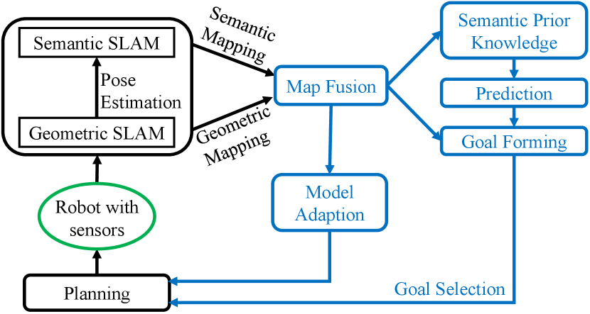
An overview of our online, real-time approach is shown in Fig. 1, where the novel contributions of this paper are highlighted in blue. The geometric SLAM and the custom semantic SLAM modules generate and update the robot pose estimation, a geometric map, and a semantic map. Using semantic prior knowledge, our system predicts the target object’s position based on the current fused map. The predicted position, together with the fused map, are fed into the goal-forming module. This module selects an intermediate goal and passes it into the planning module. The planning module uses a probabilistic planner to account for all uncertainties. Finally, as the generated plan is being executed by the robot, the SLAM modules update the map and pose estimation based on the expanded sensing information, which in turn is used to update the fused map and adapt the models of the environment and robot for the planner, forming a closed-loop system (with two loops).
Compared to existing approaches, our system’s main contributions include:
-
1.
incorporating geometric SLAM and custom semantic SLAM modules to enable full SLAM capabilities for the robot;
-
2.
incorporating prior semantic knowledge to facilitate the search of semantic objects;
-
3.
on-the-fly goal selection enabling the robot to perform exploration, more opportunistic search based on semantic objects detected, to reduce map uncertainty, or to complete the task when the target object is considered found and the mission is accomplished;
-
4.
probabilistic planning that accounts for the uncertainties in pose estimation, map, and robot motion and adapts the models for producing the policy for the next robot motion based on the ever-updated SLAM results;
-
5.
interconnections between modules so that each module is mutually dependent and mutually facilitating the related modules.
Finally, the fused maps produced in the autonomous search of a target object with our system can be used for future tasks in the same environment, and each time, the maps will be enhanced in terms of accuracy and coverage (as the robot explores more of the environment with semantic SLAM) to enable more efficient and effective robot performance in accomplishing tasks.
IV Mapping and localization
In this section, we describe how geometric and semantic SLAM is achieved, and the information from different levels is fused into a single map .
IV-A Geometric SLAM
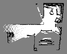
Geometric SLAM is run in parallel with semantic SLAM in our system. We employ the RTAB-MAP [35] algorithm for geometric SLAM. It generates a grid map , where and are the width and height of the grid map. , , and in the grid map represent free, occupied, and unknown space respectively, as shown in Fig. 2. The geometric SLAM module also estimates the robot pose , where and are the mean and covariance of the robot pose at time instance .
IV-B Semantic SLAM
We adapt the system introduced in our previous work [6] for semantic SLAM. At time instance , the position estimation for the semantic object is:
| (1) |
Where stands for the belief over a variable. Note that for simplicity, the subscript is dropped in (1), as in (2)–(4).
At time instance , the robot pose estimated by geometric SLAM is .
If the semantic object is detected on the color image , range-bearing measurement will be generated based on the depth information of from the depth image. The range-bearing measurement noise is:
| (2) |
The covariance of the range-bearing measurement is assumed to be time-dependent. Then the posterior belief at time can be updated using Bayes’ theorem:
| (3) |
where is a normalizing term.
Substituting the probability density functions of , , and into (3), the final result after simplification suggests that the updated posterior belief can be approximated by a multivariate Gaussian distribution :
where is the error between expected and actual range-bearing measurement,
The object class probability distribution is updated using Bayes’ rule:
| (4) |
where is a normalization constant, is the confidence level distribution of an object in different classes, returned by an object detector, such as YOLOv3 [36] at time . is one of the possible object classes. is the object detector uncertainty model, representing the probability of object detector outputs when the object class is . We use the Dirichlet distribution to model this uncertainty, with a different parameter for each object class .
IV-C Map Fusion
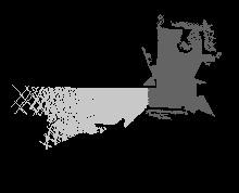
As the robot explores an environment, our system uses off-the-shelve tools [37] to segment the gradually built grid map into different geometric rooms: a room is defined as any space enclosed within a number of walls to which entry is possible only by a door or other dividing structure that connects it either to a hallway or to another room. Every grid on the grid map is assigned with a corresponding room ID: . An example is provided in Fig. 3.
Based on the locations of map objects, the corresponding geometric room IDs are assigned to the objects. Formally, a map object is represented as a 4-tuple with and the mean and covariance of the object pose, the object class distribution, and the room ID of . The object map is the set of observed map objects .
Finally, the fused map collects the grid map , object map , as well as the room information .
V Semantic Prior Knowledge
Our robot planner leverages prior semantic knowledge to facilitate efficient exploration. The key idea is that objects in the target category may have a closer affinity to some categories of objects than others. The co-occurrence relationship between objects of two categories is estimated based on Lidstone’s law of succession [38]:
| (5) |
where is the conditional probability of objects of class being in a geometric room given objects of class is already observed in the same room. is the number of times objects of classes and are observed in the same room. is the number of times objects of category are observed in a room. is a smoothing factor, and finally is the number of classes.
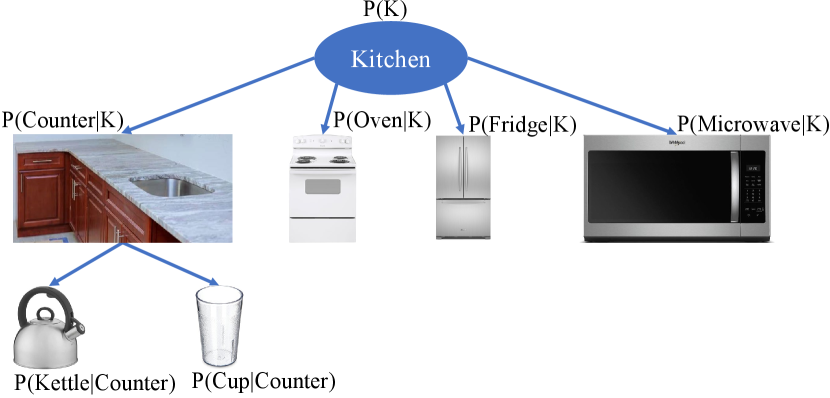
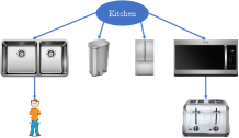
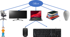
The probabilistic co-occurrence relationships of multiple pairs of objects are captured using Eq. (5) and further assembled into multiple Bayesian networks. We construct a set of Bayesian networks , with one for each semantic space . Each semantic space corresponds to one room category, such as kitchen, office, bathroom, etc. An example of a Bayesian Network is illustrated in Fig. 4, demonstrating common object classes found in a kitchen, and their conditional dependency.
For each geometric room in the environment, we will collect the set of object classes that are observed in the room . Recall that we keep a class probability distribution for each map object. Thus we cannot draw a deterministic conclusion regarding the presence of a certain object class in the room . However, to keep the problem tractable, we assume the presence of object class if for any object in the room, the probability of the object being in class exceeds some threshold : .
Given the evidence set , we only consider the Bayesian networks in that contains the target object instance and contains some objects in ; name this subset of Bayesian networks . By doing so, we narrow down the possible semantic space categories for the geometric room to a subset , which corresponds to . For each Bayesian network , our system can compute the probability of finding the target object instance in the room based on evidence , denoted as .
Our robot system can then infer the probability of finding the target object instance in the same room by feeding into the Bayesian network set :
This probability is computed for all geometric rooms.
VI Robot Modeling and Goal Forming
In this section, we describe how an intermediate goal is determined on the fly for the robot and how the intermediate goal is incorporated into the robot model as the reward signal for subsequent planning.
VI-A Robot Modeling
To account for the uncertainty in robot pose estimation, SLAM map, and robot motion, the robot is modeled as a Markov decision process (MDP) with the following components:
— is the discrete state space, representing the mean of the Gaussian distribution of the robot position. The mean of the robot’s position is discretized and clipped to the closest grid cell in the grid map to avoid an infinite state space.
— is a set of actions. We consider eight actions that allow the robot to move horizontally, vertically, and diagonally to reach its eight neighboring grid cells. A low-level controller maps the actions into the continuous robot actuation command.
— is the initial state. is determined by clipping the current robot position estimation to the nearest grid cell in the grid map .
— is the transition probability function, where represents the probability distribution over next states given an action taken at the current state . For example, for the move-up action, the robot has a high probability of moving up one cell, but it also has a small probability of moving to the upper-left or upper-right cell due to uncertainty.
— is the reward function, where is the reward for executing action at state and reaching the next state , which depends on the environment (captured by the fused map) and its changes after the robot’s action .
— is the set of (intermediate) target states, which are determined on the fly depending on the intermediate goal at the time, as described in Section VI-B.
VI-B Goal Forming and Reward Design
As the robot’s mission is to find a target object in an unknown environment, its goal of motion will be determined on the fly depending on the information provided by the fused map and the prediction made using semantic prior knowledge. The mission is accomplished if the target object is visible and identified as such.
There are several types of intermediate goals for the robot motion:
-
1.
If the target object is visible and identified as such, then the mission is accomplished and a stop signal is sent.
-
2.
If the target object is not included in the current map , the robot chooses to explore where the target object likely is. This intermediate goal requires frontier detection.
-
3.
If an object in the map may be the target object (with a low probability ), the robot chooses to observe more of the object in its visibility region and reduce the object’s uncertainty.
At the beginning of each planning cycle, the robot evaluates the mission status and decides its intermediate goal. Next, the corresponding reward function of the robot MDP model is designed to drive the robot to a selected intermediate target state based on the intermediate goal. In the following, each type of intermediate goal and the corresponding reward function is described.
VI-B1 Mission Status for Task Completion
To evaluate mission status, our robot system first identifies the object most likely in the target object category . We refer to this object as the object of interest , . If the probability of the object of interest being in the target object category exceeds a preset threshold , i.e., , then the mission is evaluated as completed, and a stop signal is sent to the planner.
VI-B2 Frontier Detection and Exploration
If the probability of the object of interest being in the target object category is smaller than a custom threshold , i.e., , the intermediate goal is to perform exploration at likely target position. The robot’s target is the frontier region . The Frontier region is the set of cells between free and unknown space in the grid map . Formally, a grid cell belongs to the frontier region if and only if and .
Our system uses the Canny edge detector [39] to detect the grid cells between free and unknown. The detected cells are grouped into edges using 8-connectivity, i.e., each cell with coordinates is connected to the cell at . Similar to map objects, a frontier edge is also assigned a single room ID based on its centroid position. The frontier region is defined as , where is the number of frontier edges. Edges with area smaller than cells are deemed as noise and excluded from . Fig. 5 shows an example frontier region in green.
The reward function is designed as:
| (6) |
where is the probability of the robot being at frontier edge if its mean position is . is the probability to find target object instance in geometric room where edge lies given the current evidence .
By including the term in the reward function, the robot is encouraged to explore frontier edges where the target object is more likely to be found. is the size of the frontier edge, representing the possible information gain by exploring . can be calculated by first discretizing the robot’s Gaussian position distribution (with mean at ) based on and then summing up the probability of the robot at each cell that belongs to . is calculated using the Bayesian network, as discussed in Section V.
VI-B3 Object Uncertainty Reduction
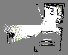
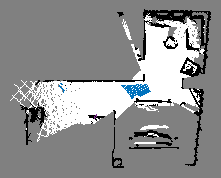
If the probability of the object of interest being in the target object category is smaller than , but greater than , i.e., , the intermediate goal is to reduce uncertainty. The robot’s target is the visibility region for the object of interest . At time , the visibility region for in the grid map with obstacles is the region of all cells on the grid map that is visible. That is, if a line connecting the position of and a cell does not intersect with any obstacle cell and is within the sensing range, then . We apply a uniform ray-casting algorithm to compute the visibility region. Rays originating from the object’s position are cast in many directions. Regions illuminated by the ray (reached by it) are considered the visibility region . An example visibility region for the current object of interest is drawn in blue in Fig. 6.
The reward function is designed as:
| (7) |
which is the probability of the robot being in visibility region if its mean position is .
VII Planning and Execution
We now describe how the optimal policy for reaching an intermediate goal is computed for the robot and how the robot will adapt to the ever-updated SLAM results.
VII-A Probabilistic Planning
The MDP and the selected reward function are fed into a planner based on the Real Time Dynamic Programming (RTDP) algorithm [40] to compute an optimal policy that maximizes the expected sum of rewards, i.e., value function . A value function starting at state following policy is defined as follows:
where is a deterministic policy over mapping the state into an action, and is a discounting factor. The optimal policy is computed as follows: for all ,
The RTDP algorithm allows us to compute a semi-optimal policy in a short time111unlike a more traditional approach such as value iteration [41].. As the robot carries out the semi-optimal policy, the policy is continuously improved by the RTDP algorithm with the current robot mean position as the initial state and converges to the optimal policy.
VII-B Adaptation
The fused map , the robot pose estimation , frontier region , and visibility region are updated at every time instance based on the ever-improving SLAM results. Consequently, once the robot reaches an intermediate target state, the MDP model must be updated. We call this process the adaptation of the MDP model. Next, the corresponding policy is also updated.
Specifically, the following components are adapted:
-
•
the discrete state space to match the changing grid map ,
-
•
the initial state to match the changing robot pose estimation ,
-
•
the transition probability function ,
- •
-
•
the set of intermediate target states as and change.
The RTDP planner takes the updated MDP model to generate a new policy.
VIII EXPERIMENTS
We conducted experiments in both simulated and real environments to verify the effectiveness and efficiency of our approach.
VIII-A Experiment Setup
In each experiment, the robot’s objective is to find any instance of the target with a confidence level greater than . The robot’s linear and angular velocity actuation signal is continuous. A task is successful if the agent has identified the target object within a specific time budget (1K seconds) and stops its motion. The set of parameters used for virtual and real-world experiments are presented in Table II.
| Parameter | Parameter meaning | Value |
| Threshold for mission completion | 0.01 | |
| Threshold for exploration | 0.5 | |
| Threshold for object evidence | 0.5 | |
| discount factor of the MDP | 0.9 | |
| Threshold for frontier region filter | 15 |
VIII-B Virtual-World Study
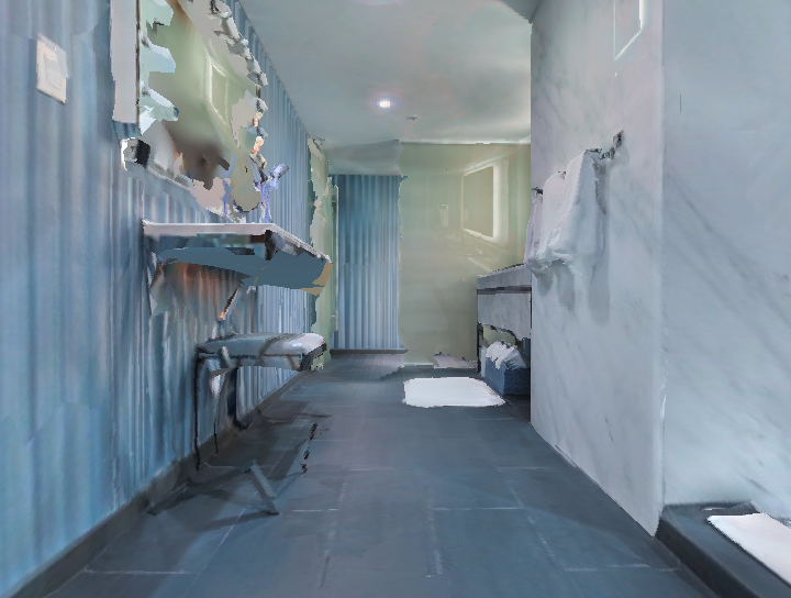
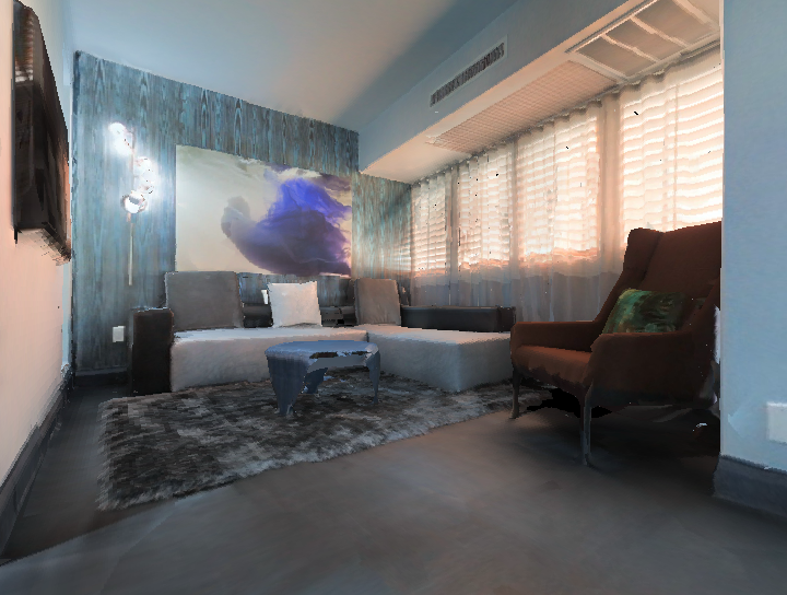
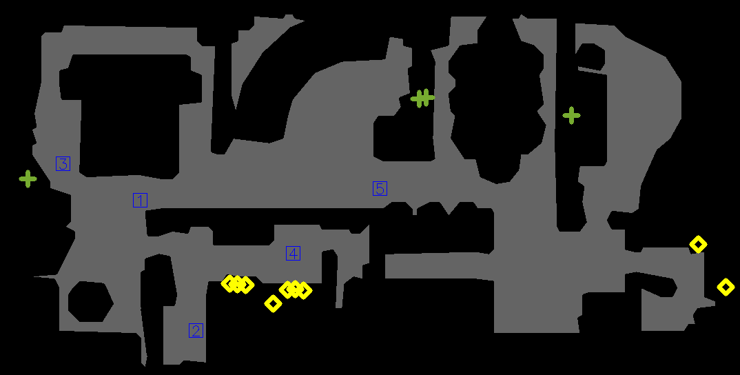
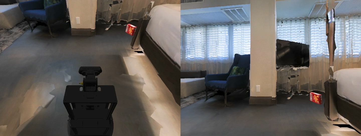
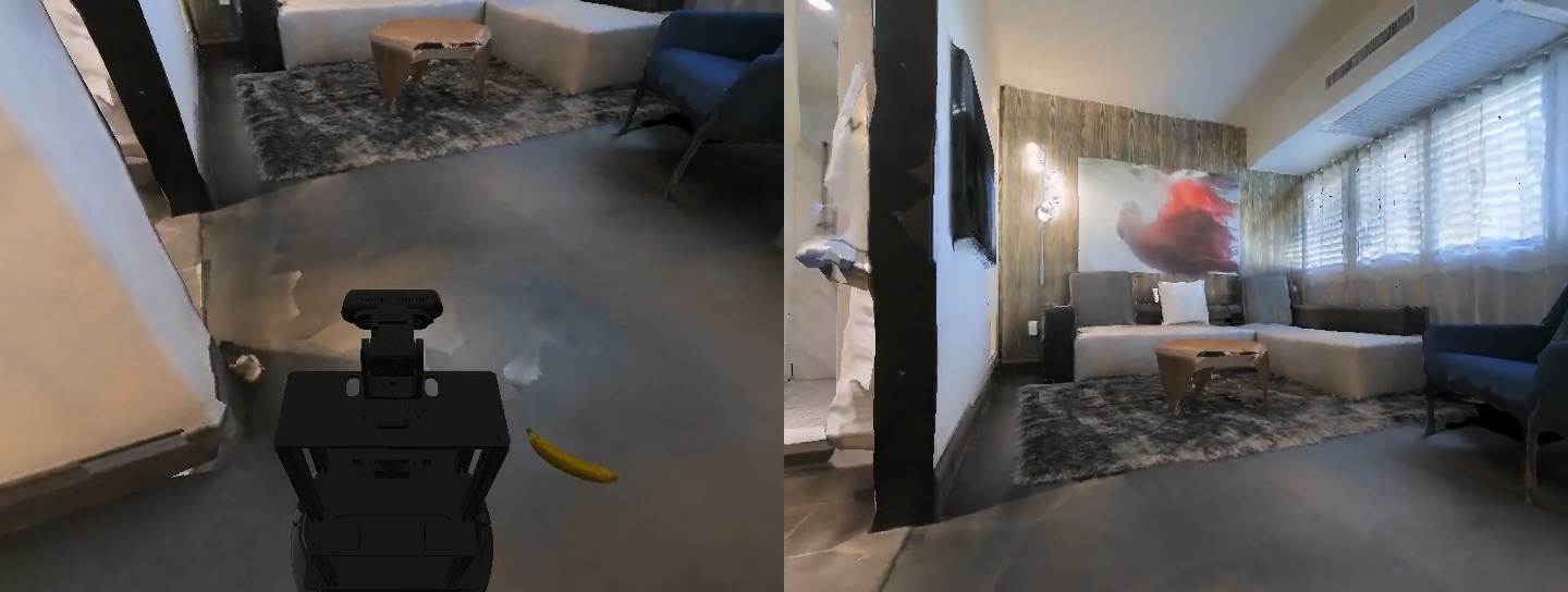
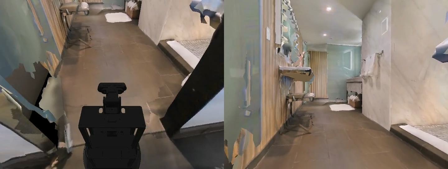
We performed experiments on the Matterport3D (MP3D) [42] dataset using the Habitat [43] simulator. MP3D dataset contains 3D scenes of a typical indoor environment, and the Habitat simulator allows the robot to navigate the virtual 3D scene. Two snapshots of the MP3D scene are given in Fig. 7. This particular scene is in size and has one level, ten rooms, and 187 objects, but it is unknown to the robot. The robot start positions and the target object instances are indicated in Fig. 8.
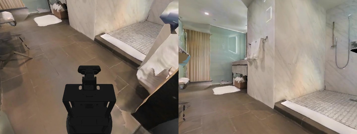
Random noise following a Dirichlet distribution is injected into the ground truth semantic labels that the Habitat-lab simulator provides to simulate the results from an object detector. Random Gaussian noise is also injected into the linear and angular velocity of the mobile robot to simulate the motion uncertainty. We used an AMD RyzenTM 3700X CPU with 3.60GHz, 16 GB of RAM, and an Nvidia GeForce RTX 3060Ti graphics card for all simulations. Fig. 9 presents several snapshots showing the robot starting from position 1 in the virtual environment at various stages of the task of finding towels.
VIII-B1 Semantic SLAM results
We present the semantic SLAM results obtained by running five task runs from starting position 1 in the MP3D dataset. Our evaluation focuses on the accuracy and uncertainty of the collected results. The results are summarized in Table III, visualized in Figs. 10 – 15, and explained in details below.
| Metrics | T1 | T2 | T3 | T4 | T5 | Average |
| MEDIAN(m) | 0.16 | 0.14 | 0.15 | 0.17 | 0.18 | 0.26 |
| MEAN(m) | 0.25 | 0.25 | 0.25 | 0.27 | 0.31 | 0.27 |
| RMSE(m) | 0.39 | 0.39 | 0.39 | 0.43 | 0.48 | 0.42 |
| Cross Entropy | 1.28 | 1.31 | 1.37 | 1.15 | 1.27 | 1.27 |
| Entropy | 1.93 | 1.80 | 1.73 | 1.75 | 1.86 | 1.82 |
| A-OPT () | 9.8 | 9.3 | 9.3 | 9.0 | 14.7 | 10.4 |
| D-OPT () | 6.95 | 6.28 | 6.29 | 7.02 | 45.7 | 14.5 |
| E-OPT () | 9.7 | 9.3 | 9.2 | 9.0 | 14.5 | 10.3 |
Accuracy
We calculate the mean and the median of the error between a predicted object’s position and the ground-truth object’s position:
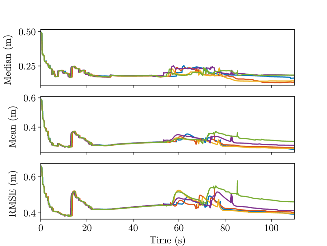
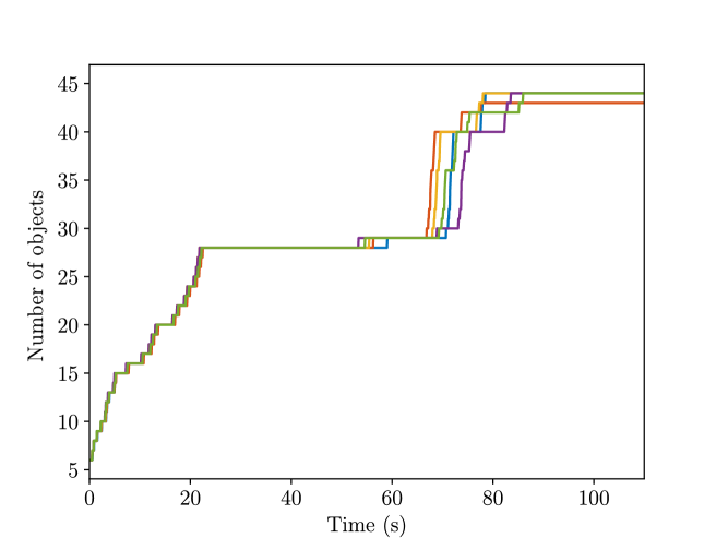
where is the current number of objects, is the estimated object position, and is the ground truth object position. Their variations over time are plotted in Fig. 10, and the final error is presented in Table III. For reference, the number of identified objects at each time instance is also plotted in Fig. 11. We can see that the error increases for the first few seconds as new objects are identified. Nonetheless, as more observations come in, the error decreases and converges. The final error in Table III is partially due to the difference between the center of object as defined by our semantic SLAM system and the ground truth. For the same reason, we expect large errors for objects with large sizes, such as tables or sofas, and we consider the median error as a more sensible metric.
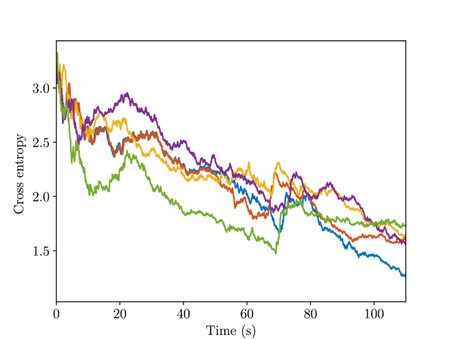
We also calculate the cross entropy between the classes of the predicted objects and those of ground-truth objects:
is the predicted object class distribution, is the ground truth of object class distribution, taking the value one at the corresponding object class and zero elsewhere. The results are plotted in Fig. 12, and the final cross-entropy is presented in Table III. We can see that the cross entropy gradually decreases with time and reaches a small value in the end, proving that the classes of the predicted objects will converge to the correct results.
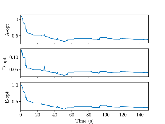
Uncertainty
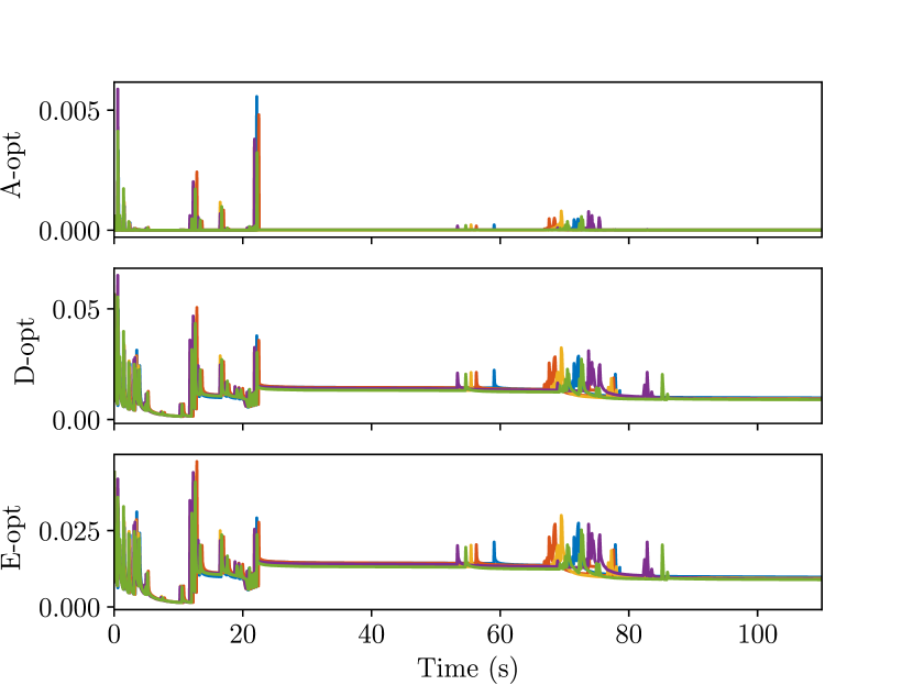
We observe a decrease in semantic map uncertainty as the robot progresses. The average A-opt (sum of the covariance matrix eigenvalues), D-opt (product of covariance matrix eigenvalues), and E-opt (largest covariance matrix eigenvalue) of the map object position covariance are calculated. Their evolution over time is plotted in Fig. 13, and the final values are stored in Table III. The spikes in the graph indicate new objects are identified, hence the increased position uncertainty. However, as time passes and more observations come in, we can see that all three metrics are kept at a low level. This shows that the robot can estimate the objects’ position fairly confidently.
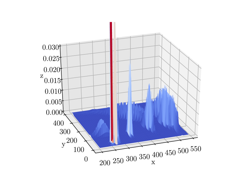
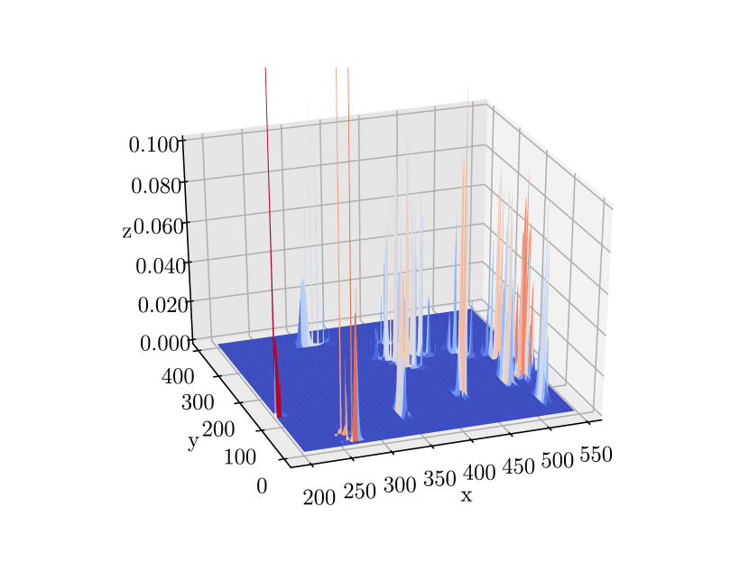
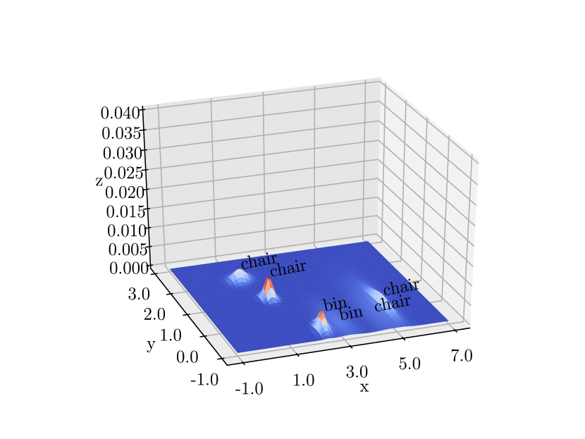
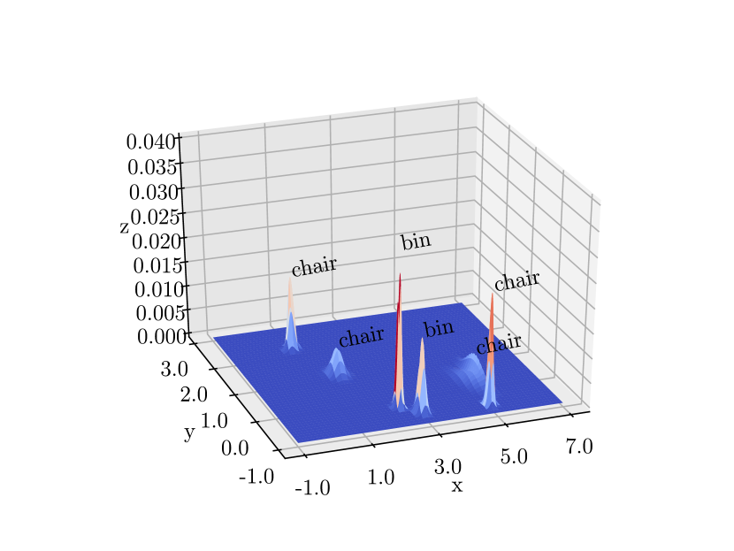
Fig. 14 gives a more intuitive representation. In Fig. 14, we plot the Gaussian functions with their means and covariances set as the estimated object position means and covariances. Therefore, each “bell” in the plot represents one object. Comparing the results we obtained at time instants and , we can see that at , the bell’s peak increases, and the base decreases, indicating a more accurate estimation of the object’s position.
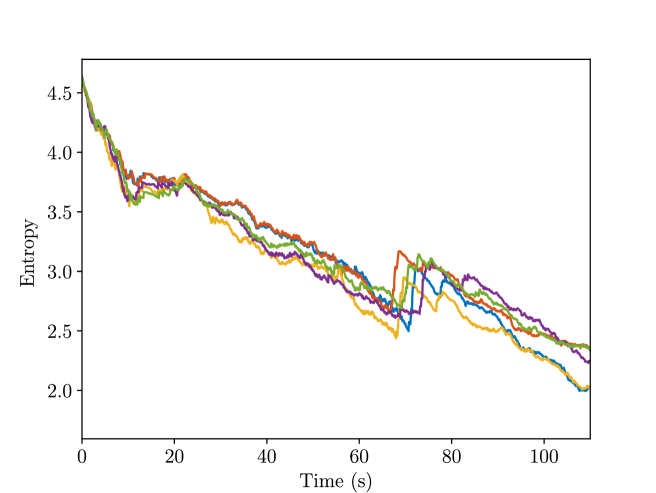
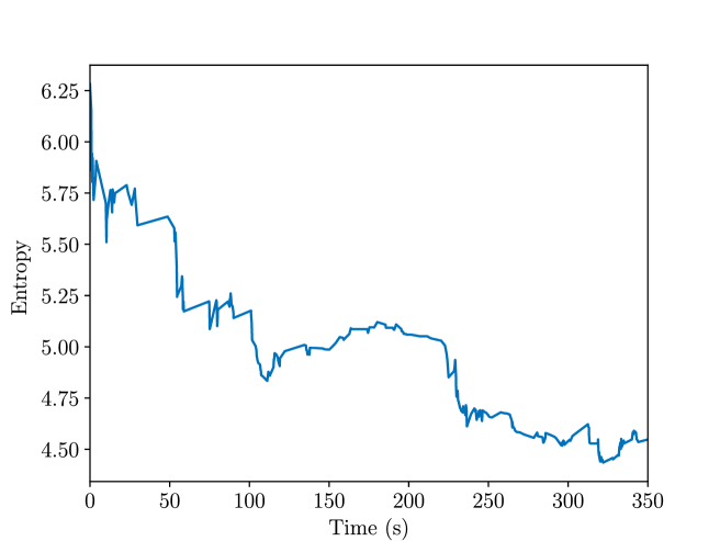
The entropy of the predicted object class is also calculated:
and visualized in Fig. 15, its final value is also listed in Table III. The result suggests that as time progresses, the robot is more and more certain about the object class it predicted.
VIII-B2 Planning results
We use the following metrics to evaluate a planner’s performance:
-
•
Success: percentage of successful task runs.
-
•
Average path length: average length of the path taken by the agent in all task runs.
-
•
Success weighted by path length (SPL) [44]:
where length of the shortest path between goal and the visibility region of target instance for a run, length of the path taken by the agent in a run, binary indicator of success in the th run.
-
•
Average time consumption: average time spent on a single task run.
Further, to establish the effectiveness of the individual components used in our planner, we conducted the following ablation studies:
-
•
Method-S: ablation of our method without semantic prior knowledge and using a uniform reward.
-
•
Method-UR: ablation of our method without uncertainty reduction.
We tested all methods on two target object categories: Towel and TV Monitor. Our system sampled five random start positions, and from each start position, it conducted five task runs. The average results are shown in Table IV.
Our method outperforms the ablation baselines in success rate, SPL, and path length by a large margin. It in turn proves the efficacy of using semantic prior knowledge to guide the search for the target object and the necessity of taking explicit actions to reduce map uncertainty.
| Category | Method | Success | Path length (m) | SPL | Time (s) |
| Towel | Our Method | 96% | 4.98 | 0.39 | 242.3 |
| Method-S | 68% | 8.73 | 0.28 | 291.7 | |
| Method-UR | 92% | 8.38 | 0.26 | 327.4 | |
| TV Monitor | Our Method | 100% | 5.75 | 0.55 | 251.7 |
| Method-S | 84% | 10.85 | 0.37 | 397.5 | |
| Method-UR | 92% | 9.19 | 0.39 | 387.2 |
VIII-C Real-World Demos
We also performed real-world experiments using a TurtleBot2 mobile robot. We deployed our algorithm on the TurtleBot and tested it in two unknown environments – involving a cluttered laboratory and a kitchen.
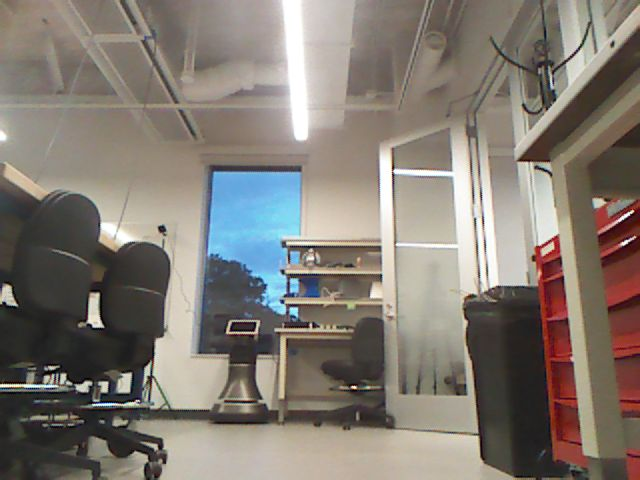
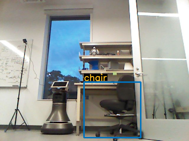
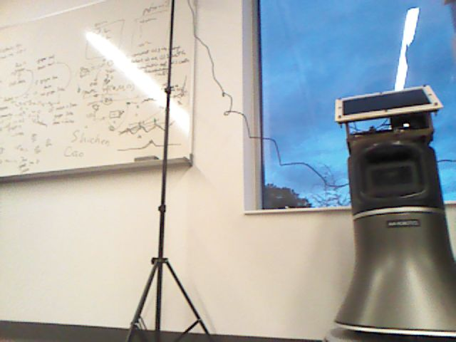
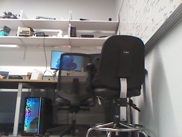
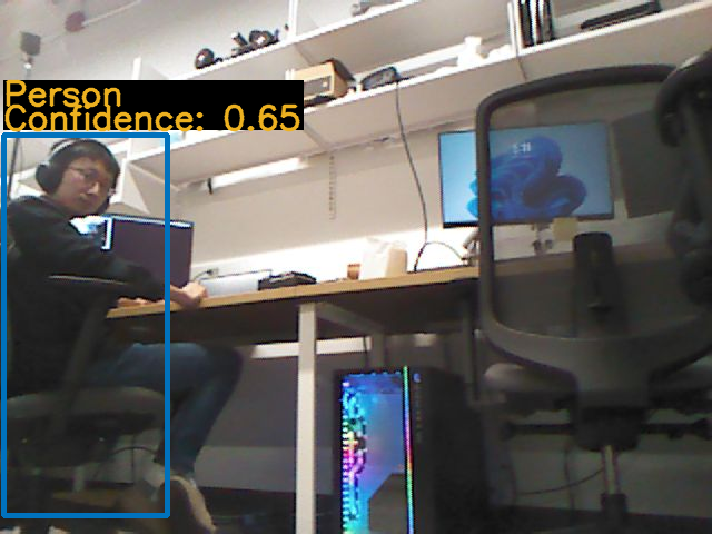
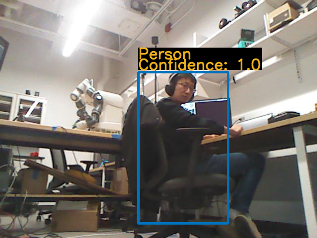
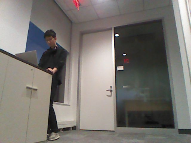
In the laboratory, the robot’s task is to find a person. The laboratory is 6m × 6m in size, unknown to the robot. Several sample images from the laboratory environment were taken from the robot’s first-person view, showing the robot at the initial position, performing exploration tasks, performing uncertainty reduction tasks, and finally identifying the target object, as shown in Fig. 16. In Fig. 16b, the robot has detected a chair in this room and inferred that a person is likely to be in the same room. From Figs. 16e and 16f, we can see that before the uncertainty reduction operation, the confidence score for the person was 0.65. After the operation, the confidence score was 1.00, and the robot correctly determined that the task was completed. The success path the robot traversed is visualized in the blue line in Fig. 17.
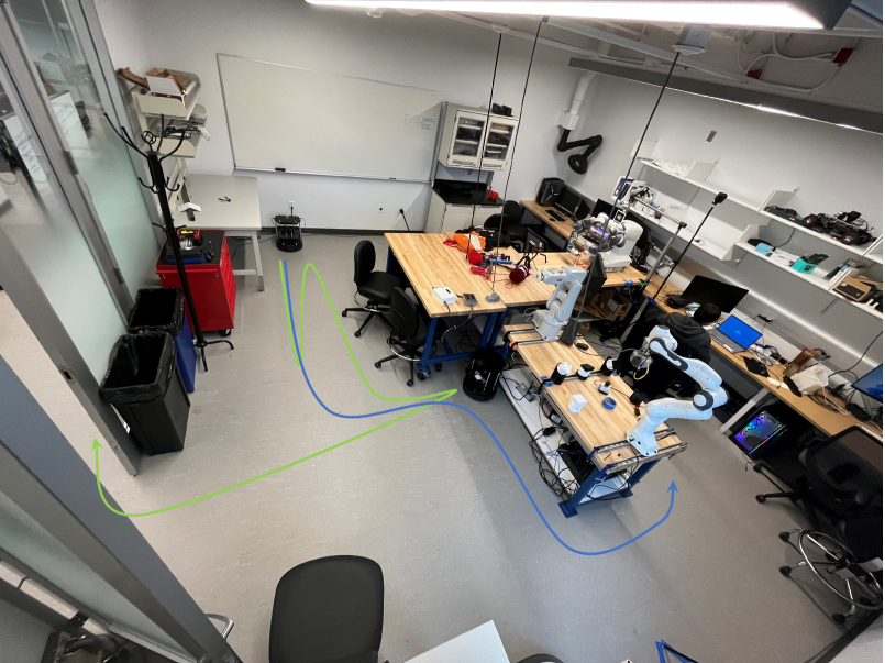
We performed three runs in the laboratory, and all were successful. The average total time for the robot to complete the task was about 4.5 minutes, and the average time spent on planning alone was seconds. The average length of the robot path was 16.3m. We estimate the optimal path to be 6.5m, which gives a SPL of 0.41.
To highlight the importance of using semantic prior knowledge, we conducted another test by denying the robot planner access to semantic prior knowledge and using a uniform reward. Without semantic prior knowledge, the robot chose to exit the laboratory and failed to find the target, as visualized in the green line in Fig. 17.
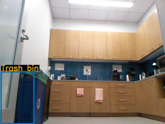
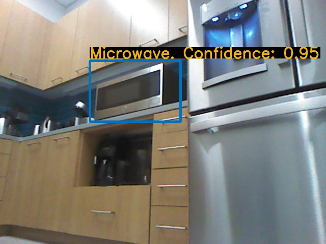
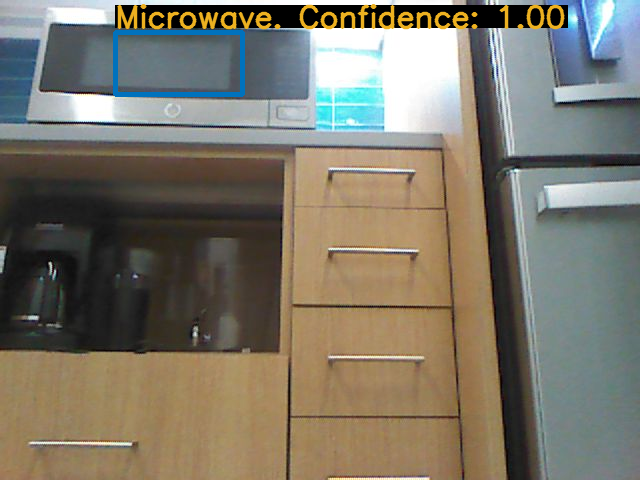
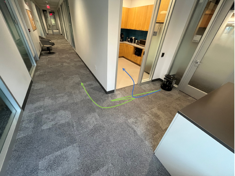
For the kitchen scenario, the robot’s task is to find a microwave. The space is about 4.5m × 5.5m in size, unknown to the robot. Several robot first-person view images from the environment are presented in Fig. 18. In Fig. 18b, the robot has detected a trash bin and inferred that the unexplored room is a kitchen and probably contains a microwave. From Figs. 18c and 18d, we can see that after the uncertainty reduction operation, the confidence score for the microwave increased from 0.95 to 1.00, and the robot correctly determined that the task was completed. The success path the robot traversed was visualized in the blue line in Fig. 19.
Again, we performed three runs in this kitchen scenario, and all three were successful. The average total time for the robot to complete the task was 7.1 minutes, and the average time spent on planning was minutes. The average length of the robot path is 13.0m. We estimate the optimal path to be 3m, which gives a SPL of 0.24.
We also conducted a test denying the robot access to semantic prior knowledge. Without semantic prior knowledge, the robot did not enter the kitchen and failed to find the target, as visualized in the green line in Fig. 19.
The real-world tests show that our approach runs effectively on a physical robot in unknown real environments, among which the lab environment has many obstacles. It enabled the robot to find the target object nested among obstacles successfully.
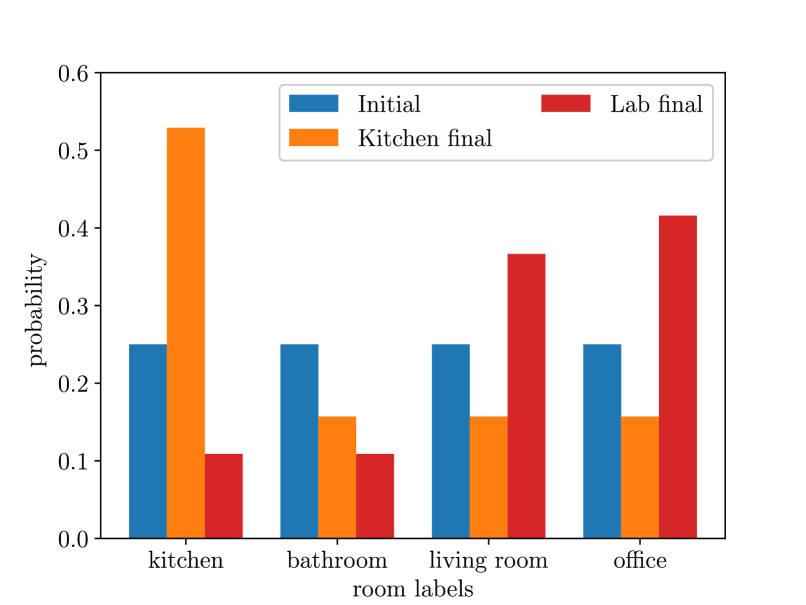
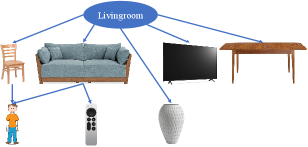
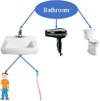
We provide the semantic room labels inferred by the Bayesian network in Fig. 20. We can see that at the beginning, due to the lack of evidence, all four room types (“Kitchen”, “Bathroom”, “living room”, “office”) were equally likely. At the end of the task, the robot correctly concluded that in the laboratory environment, the scene most resembled an office, and in the kitchen environment, the scene was most likely a kitchen. For illustration purposes, we also show the Bayesian networks used for all four room types in Fig. 21 without displaying the associated conditional probabilities for brevity.
We now present the semantic SLAM results in the lab demo. Since we do not have the object ground truth information, for the semantic SLAM results, we focus on its uncertainty reduction capability. For all the detected map objects in the lab environment, the A-opt, D-opt, and E-opt of position covariance is calculated. Their evolution over time is plotted in Fig. 22. We can see that the position uncertainty of objects decreases with time and is kept at a low level in the end.
Fig. 23 gives a more intuitive presentation. Comparing the results at time instants t = 48s and t = 70s, we can see that at t = 254s, the peak of the bell (which shows the object position covariance) increases, and the bell’s base decreases, indicating a more certain estimation of the object’s position.
The entropy of the predicted object class is visualized in Fig. 24. The result suggests that as time progresses, the robot is more and more certain about the object class it predicted.
Please refer to the supplementary video for several recorded runs in the virtual and real-world environments.
IX Conclusions
We presented a novel approach to tackle the open problem of enabling a robot to search for a semantic object in an unknown and GPS-denied environment. Our approach combines semantic SLAM, Bayesian Networks, Markov Decision Process, and Real-Time Dynamic Programming. The testing and ablation study results demonstrate both the effectiveness and efficiency of our approach. Moreover, the fused maps produced with our system can be used for performing future tasks in the same environment, and each time, the maps will be enhanced in terms of accuracy and coverage (as the robot explores more of the environment with semantic SLAM) to enable more efficient and effective task performance. In the next step, we will extend our approach to more complex, compound semantic tasks involving interaction with objects.
References
- [1] S. Thrun, W. Burgard, and D. Fox, “A probabilistic approach to concurrent mapping and localization for mobile robots,” Autonomous Robots, vol. 5, pp. 253–271, 1998.
- [2] H. Durrant-Whyte, D. Rye, and E. Nebot, “Localization of autonomous guided vehicles,” in Robotics Research, G. Giralt and G. Hirzinger, Eds. London: Springer London, 1996, pp. 613–625.
- [3] F. Fraundorfer and D. Scaramuzza, “Visual odometry: Part i: The first 30 years and fundamentals,” IEEE Robotics and Automation Magazine, vol. 18, no. 4, pp. 80–92, 2011.
- [4] D. Gálvez-López, M. Salas, J. D. Tardós, and J. Montiel, “Real-time monocular object slam,” Rob. Auton. Syst., vol. 75, pp. 435–449, 2016.
- [5] L. Nicholson, M. Milford, and N. Sünderhauf, “Quadricslam: Dual quadrics from object detections as landmarks in object-oriented slam,” IEEE Robot. Autom. Lett. (RA-L), vol. 4, no. 1, pp. 1–8, 2018.
- [6] Z. Qian, K. Patath, J. Fu, and J. Xiao, “Semantic slam with autonomous object-level data association,” in IEEE Int. Conf. Robot. Autom. (ICRA), 2021, pp. 11 203–11 209.
- [7] Z. Qian, J. Fu, and J. Xiao, “Towards accurate loop closure detection in semantic slam with 3d semantic covisibility graphs,” IEEE Robotics and Automation Letters, vol. 7, no. 2, pp. 2455–2462, 2022.
- [8] S. Yang and S. Scherer, “Cubeslam: Monocular 3-d object slam,” IEEE Trans. Robot. (T-RO), vol. 35, no. 4, pp. 925–938, 2019.
- [9] L. Zhang, L. Wei, P. Shen, W. Wei, G. Zhu, and J. Song, “Semantic slam based on object detection and improved octomap,” IEEE Access, vol. 6, pp. 75 545–75 559, 2018.
- [10] H. J. S. Feder, J. J. Leonard, and C. M. Smith, “Adaptive mobile robot navigation and mapping,” The International Journal of Robotics Research, vol. 18, no. 7, pp. 650–668, 1999.
- [11] C. Leung, S. Huang, and G. Dissanayake, “Active slam using model predictive control and attractor based exploration,” in IEEE Int. Conf. Intell. Robots Syst. (IROS). IEEE, 2006, pp. 5026–5031.
- [12] T. Kollar and N. Roy, “Trajectory optimization using reinforcement learning for map exploration,” Int. J. Robot. Res. (IJRR), vol. 27, no. 2, pp. 175–196, 2008.
- [13] A. Kim and R. M. Eustice, “Perception-driven navigation: Active visual slam for robotic area coverage,” in ICRA. IEEE, 2013, pp. 3196–3203.
- [14] S. Ehrenfeld, “On the efficiency of experimental designs,” Ann. Math. Stat., vol. 26, no. 2, pp. 247–255, 1955.
- [15] C. Stachniss, G. Grisetti, and W. Burgard, “Information gain-based exploration using rao-blackwellized particle filters.” in Robotics: Science and systems, vol. 2, 2005, pp. 65–72.
- [16] J.-L. Blanco, J.-A. Fernandez-Madrigal, and J. González, “A novel measure of uncertainty for mobile robot slam with rao—blackwellized particle filters,” IJRR, vol. 27, no. 1, pp. 73–89, 2008.
- [17] S. M. LaValle, Planning algorithms. Cambridge university press, 2006.
- [18] R. Alterovitz, S. Koenig, and M. Likhachev, “Robot planning in the real world: Research challenges and opportunities,” Ai Magazine, vol. 37, no. 2, pp. 76–84, 2016.
- [19] A. Stentz, “Optimal and efficient path planning for partially known environments,” in Intelligent unmanned ground vehicles. Springer, 1997, pp. 203–220.
- [20] S. Koenig and M. Likhachev, “Fast replanning for navigation in unknown terrain,” T-RO, vol. 21, no. 3, pp. 354–363, 2005.
- [21] J. Bruce and M. M. Veloso, “Real-time randomized path planning for robot navigation,” in Robot soccer world cup. Springer, 2002, pp. 288–295.
- [22] D. Ferguson, N. Kalra, and A. Stentz, “Replanning with rrts,” in ICRA. IEEE, 2006, pp. 1243–1248.
- [23] J. Vannoy and J. Xiao, “Real-time adaptive motion planning (ramp) of mobile manipulators in dynamic environments with unforeseen changes,” T-RO, vol. 24, no. 5, pp. 1199–1212, 2008.
- [24] Z. Wang and G. Tian, “Hybrid offline and online task planning for service robot using object-level semantic map and probabilistic inference,” Information Sciences, vol. 593, pp. 78–98, 2022.
- [25] T. S. Veiga, M. Silva, R. Ventura, and P. U. Lima, “A hierarchical approach to active semantic mapping using probabilistic logic and information reward pomdps,” in Int. Conf. Automated Planning Scheduling, vol. 29, 2019, pp. 773–781.
- [26] L. Burks, I. Loefgren, and N. R. Ahmed, “Optimal continuous state pomdp planning with semantic observations: A variational approach,” T-RO, vol. 35, no. 6, pp. 1488–1507, 2019.
- [27] S. K. Ramakrishnan, D. S. Chaplot, Z. Al-Halah, J. Malik, and K. Grauman, “Poni: Potential functions for objectgoal navigation with interaction-free learning,” in Proceedings of the IEEE/CVF Conference on Computer Vision and Pattern Recognition, 2022, pp. 18 890–18 900.
- [28] D. S. Chaplot, D. P. Gandhi, A. Gupta, and R. R. Salakhutdinov, “Object goal navigation using goal-oriented semantic exploration,” Adv. Neural. Inf. Process. Syst., vol. 33, pp. 4247–4258, 2020.
- [29] G. Georgakis, B. Bucher, K. Schmeckpeper, S. Singh, and K. Daniilidis, “Learning to map for active semantic goal navigation,” arXiv preprint arXiv:2106.15648, 2021.
- [30] C. Connolly, “The determination of next best views,” in Proceedings. 1985 IEEE international conference on robotics and automation, vol. 2. IEEE, 1985, pp. 432–435.
- [31] R. Zeng, Y. Wen, W. Zhao, and Y.-J. Liu, “View planning in robot active vision: A survey of systems, algorithms, and applications,” Comput. Vis. Media., vol. 6, no. 3, pp. 225–245, 2020.
- [32] Z. Meng, H. Sun, H. Qin, Z. Chen, C. Zhou, and M. H. Ang, “Intelligent robotic system for autonomous exploration and active slam in unknown environments,” in Int. Symp. Syst. Integr. (SII). IEEE, 2017, pp. 651–656.
- [33] M. Selin, M. Tiger, D. Duberg, F. Heintz, and P. Jensfelt, “Efficient autonomous exploration planning of large-scale 3-d environments,” RA-L, vol. 4, no. 2, pp. 1699–1706, 2019.
- [34] A. Bircher, M. Kamel, K. Alexis, H. Oleynikova, and R. Siegwart, “Receding horizon” next-best-view” planner for 3d exploration,” in ICRA. IEEE, 2016, pp. 1462–1468.
- [35] M. Labbé and F. Michaud, “Rtab-map as an open-source lidar and visual simultaneous localization and mapping library for large-scale and long-term online operation,” J. Field Robot., vol. 36, no. 2, pp. 416–446, 2019.
- [36] J. Redmon and A. Farhadi, “Yolov3: An incremental improvement,” arXiv preprint arXiv:1804.02767, 2018.
- [37] R. Bormann, F. Jordan, J. Hampp, and M. Hägele, “Indoor coverage path planning: Survey, implementation, analysis,” in ICRA. IEEE, 2018, pp. 1718–1725.
- [38] H. Schütze, C. D. Manning, and P. Raghavan, Introduction to information retrieval. Cambridge University Press Cambridge, 2008, vol. 39.
- [39] J. Canny, “A computational approach to edge detection,” IEEE Trans. Pattern Anal. Mach. Intell., no. 6, pp. 679–698, 1986.
- [40] T. Smith and R. Simmons, “Focused real-time dynamic programming for mdps: Squeezing more out of a heuristic,” in AAAI, 2006, pp. 1227–1232.
- [41] R. Bellman, “A markovian decision process,” J. math. mech., pp. 679–684, 1957.
- [42] A. Chang, A. Dai, T. Funkhouser, M. Halber, M. Niessner, M. Savva, S. Song, A. Zeng, and Y. Zhang, “Matterport3d: Learning from rgb-d data in indoor environments,” arXiv preprint arXiv:1709.06158, 2017.
- [43] M. Savva, A. Kadian, O. Maksymets, Y. Zhao, E. Wijmans, B. Jain, J. Straub, J. Liu, V. Koltun, J. Malik et al., “Habitat: A platform for embodied ai research,” in IEEE Int. Conf. Comput. Vis., 2019, pp. 9339–9347.
- [44] P. Anderson, A. Chang, D. S. Chaplot, A. Dosovitskiy, S. Gupta, V. Koltun, J. Kosecka, J. Malik, R. Mottaghi, M. Savva et al., “On evaluation of embodied navigation agents,” arXiv preprint arXiv:1807.06757, 2018.