Autoparallelity of Quantum Statistical Manifolds in The Light of Quantum Estimation Theory
Abstract
In this paper we study the autoparallelity w.r.t. the e-connection for an information-geometric structure called the SLD structure, which consists of a Riemannian metric and mutually dual e- and m-connections, induced on the manifold of strictly positive density operators. Unlike the classical information geometry, the e-connection has non-vanishing torsion, which brings various mathematical difficulties. The notion of e-autoparallel submanifolds is regarded as a quantum version of exponential families in classical statistics, which is known to be characterized as statistical models having efficient estimators (unbiased estimators uniformly achieving the equality in the Cramér-Rao inequality). As quantum extensions of this classical result, we present two different forms of estimation-theoretical characterizations of the e-autoparallel submanifolds. We also give several results on the e-autoparallelity, some of which are valid for the autoparallelity w.r.t. an affine connection in a more general geometrical situation.
Keywords— quantum estimation theory, information geometry, autoparallel submanifold, dual connection, torsion, SLD (symmetric logarithmic derivative)
1 Introduction
The autoparallelity is a multi-dimensional version (including the 1-dimensional case in particular) of the notion of geodesic for a manifold equipped with an affine connection. In the classical information geometry for manifolds of probability distributions, where the triple of the Fisher metric , the e-connection and the m-connection plays the leading role, the autoparallelity w.r.t. (with respect to) the e-connection, which is called the e-autoparallelity, is particularly important. This is because the e-autoparallel submanifolds of the space consisting of all strictly positive probability distributions on a finite set are the exponential families, which is one of the key concepts in probability theory and statistics. For quantum statistical manifolds, which are submanifolds of the space consisting of all strictly positive density operators on a finite-dimensional Hilbert space, we may introduce an analogous notion of exponential families as autoparallel submanifolds w.r.t. an affine connection on analogous to the classical e-connection. However, the notion of quantum exponential families introduced in this way does not necessarily have statistical and/or physical importance. One of the main achievements of the present paper is that the e-autoparallelity for the SLD structure, which is among a family of information-geometric structures introduced on in a unified way, has been shown to possess estimation-theoretical characterizations.
In order to clarify our motivation, we begin with an overview of a result in the classical estimation theory. Let be the totality of strictly positive probability distributions (probability mass functions) on a finite set , and let be a statistical model whose elements are smoothly and injectively parametrized by an -dimensional parameter ranging over an open subset of . As is well known, the variance matrix of an arbitrary unbiased estimator for the parameter satisfies the Cramér-Rao inequality , where denotes the Fisher information matrix. An unbiased estimator achieving the equality for every is called an efficient estimator for the parameter , whose existence is known to impose strong restrictions on both the set and the parametrization . Namely, we have the following theorem (e.g. § 5a.2 (p.324) of [1], Eq. (7.14) in § 7.2 of [2], Theorem 3.12 of [3]).
Theorem 1.1.
For a statistical model , the following conditions are equivalent.
-
(i)
There exists an efficient estimator for the parameter .
-
(ii)
is an exponential family, and is an expectation parameter.
Condition (ii) in the above theorem means that the elements of are represented as
| (1.1) |
and that the parameter satisfies
| (1.2) |
where denotes the expectation w.r.t. the distribution . This condition is expressed in the language of geometry as follows.
-
(ii)’
is autoparallel in w.r.t. the e-connection of , and forms an affine coordinate system w.r.t. the m-connection of .
Remark 1.2.
In the notation of [3] as well as of many references on information geometry, , and in (1.1) and (1.2) are expressed as , and , respectively. The reason why the upper and lower indices are reversed here (and throughout the paper) is that we first treat as an arbitrary coordinate system, which has an upper index (superscript) as in the standard notation of differential geometry, and then consider the condition for to become an m-affine coordinate system such as the expectation coordinate system.
A quantum version of Theorem 1.1 is known, which we state below. Let be a finite-dimensional Hilbert space, be the totality of strictly positive density operators on , and be an arbitrary quantum statistical model consisting of states in . It is well known that the variance matrix of an arbitrary unbiased estimator for the parameter satisfies the SLD Cramér-Rao inequality [6, 7], where is the SLD Fisher information matrix (see Section 4 for details.) When an unbiased estimator satisfies for every , we call it an efficient estimator for the parameter as in the classical case. Then we have the following theorem (Theorem 7.6 of [3]).
Theorem 1.3.
For a quantum statistical model , the following conditions are equivalent.
-
(i)
There exists an efficient estimator for the parameter .
-
(ii)
There exist mutually commuting Hermitian operators and a strictly positive operator such that the elements of are represented as
(1.3) and that
(1.4)
When a model is represented as (1.3), we call it a quasi-classical exponential family. As is pointed out in [3] and will be verified in Section 4 of this paper, a quasi-classical exponential family is e-autoparallel in w.r.t. the SLD structure. Note, however, that this is merely a special case of e-autoparallel submanifolds. Namely, the existence of efficient estimator is too strong as a characterization of the e-autoparallelity. Is it then possible to characterize the e-autoparallelity by an estimation-theoretic condition which is weaker than the existence of efficient estimator? We give an affirmative answer to this question in Section 5. We also give another characterization of the e-autoparallelity in Section 7 by considering estimation for scalar-valued functions instead of estimation for vector-valued parameters.
As mentioned above, the e-autoparallelity in the SLD structure has estimation-theoretical significance and is therefore a concept worth studying further. It should be noted here that the e-connection in the SLD structure is curvature-free but not torsion-free, so that the e-connection is not flat. This also means that is not a dually flat space w.r.t. the SLD structure. In the case of a flat connection, an autoparallel submanifold corresponds to an affine subspace in the coordinate space of an affine coordinate system, so that the existence condition for autoparallel submanifolds is obvious. For a non-flat connection, on the other hand, we cannot see the whole picture of autoparallel submanifolds and are faced with the new problem of what kind of condition ensures the existence of autoparallel submanifold. Therefore, it is also important to study the autoparallelity from a purely geometrical point of view, away from estimation problems. This is another concern in this paper, along with the estimation-theoretical consideration.
The paper is organized as follows. In Section 2, we explain the basic issues about the autoparallelity for an affine connection on a general differential manifold, focusing in particular on the situation where the dual connection of w.r.t. a Riemannian metric is flat. In Section 3, we introduce a family of information-geometric structures on the space , and derive the basic issues concerning the e-autoparallelity by applying the results of Section 2. These two sections are preliminaries for later sections. Although the results shown there are mostly known, we present them together with their derivations so that the descriptions are as self-contained as possible. Section 4 also consists of basically known results, where Theorem 1.3 is revisited, and it is clarified that the existence of efficient estimator only partially characterizes the e-autoparallelity for the SLD structure. This observation motivates Section 5, where a sequence of estimators, which is called a filtration of estimators, is treated instead of a single estimator, and the existence of efficient filtration is shown to characterize the e-autoparallelity. In Section 6, it is shown that a quantum Gaussian shift model has an efficient filtration and that the model in fact exhibits an analogous property to the e-autoparallelity in , although the Hilbert space is infinite-dimensional in this case, so that we cannot fully develop a differential geometrical argument there. Section 7 treats an estimation problem for scalar-valued functions, where it is shown that a quantum statistical manifold is e-autoparallel in if and only if the linear space formed by functions having efficient estimators is of maximal dimension. In Section 8, we move away from estimation theory and consider the condition for existence of e-autoparallel submanifolds from a purely geometrical point of view, where the involutivity of a parallel distribution of tangent spaces is studied in relation to the torsion tensor. In Section 9, we treat the case when and study the SLD structure of the space of qubit states. It is shown there that in this case has a characteristic property that every e-parallel distribution is involutive. Section 10 is devoted to concluding remarks. Some proofs and additional results are included in Appendix for the sake of readability of the main text.
Remark 1.4.
We make some remarks on the nomenclature and the notation of the paper.
-
1.
Throughout the paper, when we refer to a manifold, say , it means that is a manifold with a trivial global structure, so that we need not worry about the difference between global properties and local properties of . For instance, is always supposed to have a global coordinate system, and every closed differential form on is considered to be exact.
-
2.
When we say that is a coordinate system of a manifold in the subsequent sections, it basically means that is a map (a global chart of ) which represents each point by an -dimensional vector , although the same symbol has appeared above as a parameter to specify a point in the manifold. They are equivalent by . A parametrization is often more convenient than a coordinate system when dealing with concrete examples. In fact, we will use parametrizations in Section 6 for quantum Gaussian states and in Section 9 for qubit states.
-
3.
This paper contains both arguments on quantum statistical manifolds (manifolds consisting of density operators) and those on general manifolds. We denote quantum statistical manifolds by , while general manifolds are denoted by .
2 Basic issues about autoparallelity
In this section we summarize basic issues related to autoparallelity from the perspective of general differential geometry, which will be necessary for later discussions.
Let be an arbitrary manifold, and denote the totality of smooth functions and that of smooth vector fields on by and , respectively. Suppose that is provided with an affine connection , which is a map . Given a submanifold of , let denote the totality of smooth mappings which map each point to a tangent vector in , i.e., sections of the vector bundle . Then naturally induces a map so that for any and any , is defined as an element of . Since , is defined for any , although it does not necessarily belong to .
When belongs to for every , is said to be autoparallel w.r.t. or -autoparallel in (e.g., Sec. 8 in Chap. VII of [4]). In particular, itself is -autoparallel in . An autoparallel curve is usually called a geodesic (or pregeodesic when we wish to clarify that our interest lies only in the image of the curve), so that the autoparallelity is a multi-dimensional extension of the notion of geodesic. When is -autoparallel in , defines an affine connection on . We denote this connection by when we wish to distinguish it from the original connection on . The autoparallelity is transitive in the sense that if is -autoparallel in and is -autoparallel in , then is -autoparallel in .
Remark 2.1.
If is -autoparallel in and is a nonempty open set of , then is also -autoparallel in having the same dimension as . In this paper, we restrict ourselves to maximal autoparallel submanifolds to avoid this ambiguity. In particular, an autoparallel submanifold of having the same dimension as is considered to be only . This restriction is merely for simplicity of descriptions.
Remark 2.2.
A similar but different notion to autoparallelity is total geodesicness. A submanifold is said to be totally geodesic w.r.t. or -totally geodesic in when for any point and any tangent vector of , the -geodesic passing through in direction lies in . It is obvious that the autoparallelity implies the total geodesicness, but the converse is not true in general except when is torsion-free ([4], Theorem 8.4 in Chap. VII). We will revisit this topic in Remark 8.6.
A vector field is said to be parallel w.r.t. or -parallel when . More generally, (including the case ) is said to be -parallel when .
When there exist on the same number of linearly independent -parallel vector fields as , we say that is curvature-free. This condition is known to be equivalent to the curvature tensor of vanishing on . When is curvature-free, the parallel transport is defined for arbitrary two points so that a vector field is -parallel iff .
The following two propositions are straightforward, where the curvature-freeness is essential.
Proposition 2.3.
For a submanifold of on which a curvature-free connection is given and for (including the case when ), the following conditions are equivalent.
-
(i)
is -parallel.
-
(ii)
, is -parallel and .
Proposition 2.4.
For an -dimensional submanifold of on which a curvature-free connection is given, the following conditions are equivalent.
-
(i)
is -autoparallel in .
-
(ii)
.
-
(iii)
There exist linearly independent -parallel vector fields on .
-
(iv)
There exist linearly independent -parallel vector fields on such that , .
When these conditions hold, a vector field on is -parallel iff it is -parallel, and is curvature-free.
In the following, we consider the case when is additionally provided with a Riemannian metric for which the dual connection of is flat. Namely, the triple satisfies the duality [5] [3]:
| (2.1) |
and is flat in the sense that it is curvature-free and torsion free. The flatness is known to be equivalent to the existence of a coordinate system , which is called an affine coordinate system w.r.t. , such that , are all -parallel. In this case, turns out to be curvature-free, since the curvature-freeness is preserved by the duality of connections (Theorem 3.3 of [3]), but is not necessarily torsion-free, and hence is not necessarily dually flat.
Proposition 2.5.
In the above situation, we have:
-
(1)
For a vector field , is -parallel iff is constant on for every -parallel vector field .
-
(2)
For a vector field , is -parallel iff is constant on for every -parallel vector field .
Proof The proposition relies not on the torsion-freeness of but only on the curvature-freeness of and , so that it suffices to show (1). For an , we have
| is -parallel | ||||
| (2.2) |
where in follows since the set of -parallel vector fields has the same dimension as due to the curvature-freeness of , and follows since the duality (2.1) and the -parallelity of implies
| (2.3) |
Suppose that is -autoparallel in . Then is a Riemannian submanifold of equipped with the affine connection . Hence the dual connection of w.r.t. (more precisely, w.r.t. the induced metric on ) is defined, which we denote by ; i.e.,
| (2.4) |
where we have applied . From (2.1) and (2.4), we have
| (2.5) |
which means that is the -projection of onto .
Since the curvature-freeness and the torsion-freeness are respectively preserved by the duality and the projection, is flat as in the case with , which ensures the existence of -affine coordinate system of .
The following proposition will be of fundamental importance for later arguments.
Proposition 2.6.
For an -dimensional submanifold of and a coordinate system of , the following conditions are equivalent.
-
(i)
is -autoparallel in , and is a -affine coordinate system.
-
(ii)
For every , the vector field
(2.6) is -parallel, where and .
Proof We first show (i) (ii). Assume (i) and define by (2.6). Then we have for every , which is constant on . Noting that vector fields are -parallel and that Prop. 2.5 can be applied to due to the -autoparallelity of , it follows from item (1) of Prop. 2.5 that is -parallel, and hence it is -parallel.
3 Information geometric structures on quantum statistical manifolds
In this section, we introduce the information-geometric structures on quantum statistical manifolds and apply the results of the previous section to them. The geometric structure treated here is essentially the same as the one studied in § 7.3 of [3].
Let , and be the totality of linear operators on , that of Hermitian operators on and that of strictly positive density operators on , respectively. Then is an open subset of the affine space , so that a flat affine connection is naturally introduced on , which we call the m-connection and denote by . In order to express more explicitly, we introduce the embedding map so that is denoted by when treating it as an element of . Since is a smooth map, it has the differential at every point , which we denote by . For a vector field , the map is defined to be . Then the definition of the m-connection is represented as follows:
| (3.1) |
where is the derivative of w.r.t. . When a coordinate system is arbitrarily given and the elements of is parametrized by it as , we have
| (3.2) |
and
| (3.3) |
where .
Suppose that we are given a family of inner products on the -linear space , where the correspondence is smooth, and assume that
| (3.4) |
The inner products are represented as
| (3.5) |
by a family of super-operators , where denotes the Hilbert-Schmidt inner product. Note that the assumption (3.4) is equivalent to
| (3.6) |
For an arbitrary tangent vector , a Hermitian operator is defined by the relation
| (3.7) |
where the LHS denotes the derivative of the function , w.r.t. . Noting that the LHS and the RHS are represented as and , respectively, we can rewrite (3.7) into
| (3.8) |
| (3.9) |
Since are one-to-one correspondences, we obtain the following identity:
| (3.10) |
In the following, we often express (3.4) as
| (3.11) |
as an identity for functions on . Similarly, (3.7) is expressed as
| (3.12) |
where is a vector field on , denotes the map , , and denotes the function .
For a submanifold of and a vector field on it, the map is defined, for which (3.12) holds as an identity for functions on . We may write as in this case. In particular, given a coordinate system of , we have
| (3.13) |
where and .
Remark 3.1.
In the terminology of [3], and are called the m-representation and e-representation, and are denoted by and , respectively. We do not use the symbols and in this paper, but may use the following notation when convenient:
| (3.14) | ||||
| (3.15) |
Note that
| (3.16) |
Now, we define a Riemannian metric on by
| (3.17) |
which is equivalently written as
| (3.18) |
We also have the expression
| (3.19) |
where , , denotes the derivative of the map , , w.r.t. , and denotes the function . This expression is derived as
| (3.20) |
where the first equality follows from (3.9) and the last from (3.7), with dots added to clarify the positions of variables of maps. An important class of such Riemannian metrics is that of monotone metrics [9] for which is represented as
| (3.21) |
where is an operator monotone function satisfying and , and is the modular operator defined by . The class contains the SLD metric, which plays the main role in this paper, defined by and
| (3.22) |
where denotes the symmetrized product: . In this case, (, resp.) is called the SLD (symmetric logarithmic derivative) of the tangent vector (the vector field , resp.). In particular, obeys the equation
| (3.23) |
which is a popular expression for the SLD.
Given a family of inner products which determines a Riemannian metric , let the e-connection be defined as the dual connection of w.r.t. ; i.e.,
| (3.24) |
We have thus obtained as an example of treated in the previous section, where and are dual w.r.t. , is curvature-free and is flat. The triple is called the information-geometric structure on induced from a family of inner products . In particular, the information-geometric structure induced from the symmetrized inner product (3.22) is called the SLD structure. It is the SLD structure that will play a leading role in subsequent sections in relation to estimation theory, but this section will continue the discussion on general information-geometric structures.
Remark 3.2.
As is shown in Theorem 7.1 of [3], there is only one information-geometric structure defined in the manner described above for which the e-connection is torsion-free (so that is dually flat). That is the structure induced from the BKM (Bogoliubov-Kubo-Mori) inner product
| (3.25) |
The induced Riemannian metric is a monotone metric corresponding to . In the other cases, the torsion does not vanish, where denotes the Lie bracket for vector fields.
Remark 3.3.
For the SLD structure, it is known ([3], Eq. (7.80)) that the torsion has the following representation : for each point and each tangent vectors , we have
| (3.26) |
where in the RHS denotes the commutator for operators on . Since this representation will be used in Sections 8 and 9, we show its proof in A1 of appendix for the reader’s convenience.
Henceforth, we use the prefixes e- and m- for notions concerning the e-connection and m-connection; e.g., e-parallel, e-autoparallel, m-affine, etc.
Proposition 3.4.
For any vector fields , we have
| (3.27) |
Proof Differentiating (see (3.18)) by , we have
where the second equality follows from (3.1). Letting be defined by , whose existence is ensured by (3.10), the above equation is represented as
This means that , and proves the proposition.
Proposition 3.5.
For a vector field , we have
| is e-parallel | ||||
| (3.28) |
Proof We may use Prop. 3.4 to prove this, but here we show an alternative proof. We first note that, according to (3.1), a vector field is m-parallel if and only if is a constant map represented by an operator as . Invoking Prop. 2.5, we have
| is e-parallel | |||
Recalling Prop. 2.3, the following corollary is immediate.
Corollary 3.6.
For a submanifold of and for (including the case when ), we have
| is e-parallel | ||||
| (3.29) |
The following corollary is also immediate from Prop. 3.5.
Corollary 3.7.
The e-parallel transport for arbitrary two points is represented as follows: ,
| (3.30) |
In the following, a pair of a submanifold of and a coordinate system of is called a model.
Proposition 3.8.
For an -dimensional model , the following conditions are equivalent.
-
(i)
is e-autoparallel in , and is an m-affine coordinate system.
(Note: “m-affine” means “affine w.r.t. the m-connection on ”.) -
(ii)
such that for every
(3.31) where , and .
- (iii)
- (iv)
Proof The equivalence (i) (ii) is immediate from Prop. 2.6 and Cor. 3.6, and (iii) (ii) is obvious since .
To show (ii) (iii), assume (ii). Then we have
Here, the LHS is and the RHS is due to (3.13). Hence, there exists a constant vector such that . Redefining , (3.31) is rewritten as (3.32), and (iii) is verified.
Since (3.32) implies that
we have (iii) (iv). To show the converse, we assume the existence of in (iv). Then we have , and for each there exist and such that for any
This implies that
Hence we have
Here, the constant should be equal to due to . Thus (iii) is concluded.
Remark 3.9.
At the end of this section, we present a proposition which claims that i.i.d. extensions of a model preserves the e-autoparallelity. For the proposition, we assume the following condition on the family of inner products from which the information-geometric structure is defined:
| (3.34) |
which is equivalent to
| (3.35) |
The assumption is satisfied when the inner products are defined from a function by (3.5) and (3.21) for which and hold. In particular, the proposition hols for the SLD structure.
Proposition 3.10.
Proof Let , , and , , which are determined by
and
where denotes the natural embedding . With the aid of the parametric representation (3.2), we see that
where follows from (3.6) and (3.35), and we have used the notation
This implies that and that for and , which leads to . Hence, and are linked by Now, according to Prop. 3.8, conditions (i), (ii) of the present proposition are respectively expressed as
-
(i)’
.
-
(ii)”
.
They are obviously equivalent with relation .
4 Efficient estimators
From this section, we investigate the relationship between estimation problems and geometric properties for quantum statistical models. Henceforth, we will consider only the SLD structure as an information geometric structure unless otherwise stated.
Given a model in , an estimator for coordinates is generally represented by a POVM on , where is a variable representing an estimate. A representative case is when is expressed as by a POVM on a finite set and a function , where denotes the -measure concentrated on the point . This estimator, which is denoted by , represents the estimation procedure in which the estimate is determined as from the outcome of the measurement .
The expectation and the mean squared error (the variance in the unbiased case) of for a state are defined by
| (4.1) | ||||
| (4.2) |
where is regarded as the space of column vectors and T denotes the transpose. For , we have
| (4.3) | ||||
| (4.4) |
An estimator is called locally unbiased for a coordinate system at when the elements , , of satisfy
| (4.5) |
where denotes the derivative of the function by evaluated at the point . We denote by the totality of locally unbiased estimators for at . Using the symmetrized inner product of (3.22) and the SLDs , , we have
| (4.6) |
where
| (4.7) |
The well-known SLD Cramér-Rao inequality [6, 7] states that every obeys
| (4.8) |
where denotes the SLD Fisher information matrix defined by , where is the SLD metric. Furthermore, the following proposition holds.
Proposition 4.1.
For every column vector , we have
| (4.9) |
Note that in (4.9) cannot be replaced with in general.
Let us introduce a class of randomized procedures for estimation that will be useful in the proofs of both Prop. 4.1 above and Theorem 5.1 later. Suppose that a point , a basis of , a positive probability vector s.t. , and real numbers satisfying
| (4.10) |
are arbitrarily given. Let
| (4.11) |
where , , , and consider the random measurement such that is randomly chosen according to the probability distribution and then the observable is measured. This measurement is represented by the POVM , where are the projectors in the spectral decomposition . (Do not confuse , and with the th powers of , and .) When an eigenvalue is observed by measuring , we estimate by , where is defined by
| (4.12) |
and , i.e., and . This estimation procedure defines the estimator , which is characterized by the following property: for any polynomial function ,
| (4.13) |
In this situation we have the following lemma, whose proof is given in A2 of Appendix.
Lemma 4.2.
The estimator satisfies:
-
(1)
.
-
(2)
,
where .
Proof of Prop. 4.1 Let , which satisfies (4.10) so that Lemma 4.2 is applicable. Since in this case, we have
The proposition is obvious when , so we assume and choose arbitrarily. Taking and in the above construction such that and , the resulting satisfies . Since can be arbitrarily close to , we have the proposition.
A locally unbiased estimator is called locally efficient for at if for all . Given a positive-semidefinite matrix as a weight, an estimator is called locally -efficient for at if for all , or equivalently if
| (4.14) |
Here, the symbol is used for the trace of matrices to distinguish it from the trace for operators on .
Proposition 4.3.
Given a model , a point and an estimator , the following conditions are equivalent.
-
(i)
is locally efficient for at .
-
(ii)
.
-
(iii)
is locally -efficient for at for every column vector .
-
(iv)
is locally -efficient for at for every positive weight .
Remark 4.4.
As is well known, there exists a locally efficient estimator at iff the SLDs mutually commute (e.g. § 7.4 of [3]).
An estimator is called efficient for a coordinate system if is locally efficient for at every point . Given a weight field , is called -efficient for if is locally -efficient for at every . When for all , we simply call it -efficient for . According to Prop. 4.3, is efficient is -efficient for every is -efficient for every .
The condition for existence of efficient estimator was mentioned in the introduction as Theorem 1.3. Suppose that is represented as (1.3) and (1.4) in the theorem; namely, every is represented in the form
| (4.15) |
and satisfies , where are mutually commuting observables. Note that can be chosen to be an arbitrary element of if we wish. The SLDs of w.r.t. are represented as
| (4.16) |
where and . Noting that the positions of upper/lower indices (superscripts and subscripts) are reversed from the standard notation of information geometry as in [3] (see Remark 1.2), we have , and
| (4.17) |
According to Prop. 3.8, this means that is e-autoparallel in and that is an m-affine coordinate system w.r.t. the SLD structure. Furthermore, the induced e-connection on turns out to to be torsion-free and hence flat, for which forms an affine coordinate system. We have thus seen that is dually flat just as classical exponential families.
When , (4.15) is written as
| (4.18) |
This is a general form of e-geodesic in the sense that every e-geodesic is represented in this form by some and . In the multi-dimensional case , on the other hand, (4.15) provides merely a special case of e-autoparallel submanifolds. In order to characterize the e-autoparallelity by an estimation-theoretical notion, the existence of efficient estimator is too strong, and we need a new variant of the notion of efficient estimators, which will be introduced in the next section.
5 Efficient filtration of estimators
We now consider a one-parameter family of estimators instead of a single estimator, and call it a filtration of estimators or simply a filtration. The upper limit can be an arbitrary positive number or , but our interest lies only in the limiting property of and the value of plays no role. So we simply write . Given a nonnegative real matrix as a weight, a filtration is called locally -efficient for at if for every and for every , which is equivalent to
| (5.1) |
When with , in particular, this is represented as
| (5.2) |
due to Prop. 4.1. Compare (5.1) with (4.14), and note that a locally -efficient filtration at always exists, even when a locally -efficient estimator does not exist.
Given a weight field , a filtration is called -efficient for if it is -locally efficient for at every . When for all , we simply call it -efficient for .
Now, we have the following theorem, which gives an estimation-theoretical characterization of the e-autoparallelity.
Theorem 5.1.
For a model , the following conditions are equivalent.
-
(i)
is e-autoparallel in , and is an m-affine coordinate system.
-
(ii)
For every , there exists a -efficient filtration for .
Proof According to Prop. 3.8, it suffices to show the equivalence of (ii) and the condition that
| (5.3) |
where .
We first show (ii) (5.3). Fix arbitrarily, and let be an -efficient filtration for , where denotes the th vector of the natural basis of . For each , we have
| (5.4) |
where
and denotes the norm for the symmetrized inner product . (We also denote the norm for the metric by the same symbol.) From the local unbiasedness condition (4.6) applied to , we have
This means that is the orthogonal projection of onto . Hence we have
| (5.5) |
The -efficiency of is represented as
which, combined with (5.4) and (5.5), yields
This implies that a -independent Hermitian operator exists and satisfies for every , which concludes (5.3).
We next show (5.3) (ii). Let be arbitrarily given, for which we will construct -efficient filtration by assuming the existence of of (5.3). We can assume , and take a basis , , of such that , whereby for each we define
| (5.6) |
Let , and take a positive probability vector such that . We define the estimator by the following estimation procedure: randomly choose according to the probability distribution , measure the observable to get an outcome , and then estimate by using the function defined by
| (5.7) |
where . Invoking (5.3) evaluated at an arbitrary point , we have
where and are those defined by (4.11) and (4.12) with
| (5.8) |
Since this satisfies (4.10), Lemma 4.2 applies to conclude that is locally unbiased at and satisfies, for every and every ,
| (5.9) |
where . From (5.8), we have
and hence
Thus, letting in (5.9), we obtain
This implies that for every and that is a -efficient filtration.
Proposition 5.2.
In the situation of Prop. 3.10 where is the th i.i.d. extension of , has an efficient filtration if and only if has an efficient filtration.
6 A sufficient condition for the e-autoparallelity and its relation to the Gaussian states
Proposition 6.1.
For a model , the following condition is sufficient for (i) and (ii) of Theorem 5.1:
-
•
For every positive weight , there exists a -efficient estimator for .
Proof Given and , arbitrarily, let be a -efficient estimator. Then, for an arbitrary and an arbitrary , we have
This implies that for every , so that the filtration is -efficient.
An important example of a model satisfying the condition of Prop. 6.1 is given by a model consisting of quantum Gaussian states. Strictly speaking, the model is mathematically out of our scope in that the underling Hilbert space is infinite-dimensional. Nevertheless, it is worthwhile to consider the relationship between this important model and the e-autoparallelity, even at the expense of some rigor.
We begin by quickly reviewing the definition of quantum Gaussian states based on the description in Chapter 5 of [8]. Let be an even-dimensional real linear space on which a symplectic form is given, and be an irreducible projective representation of on a separable Hilbert space ; i.e., is a family of unitary operators on satisfying , and having no nontrivial invariant subspace. For each , a self-adjoint operator is defined by , and satisfies
| (6.1) |
Given a symmetric bilinear form on satisfying , and a linear functional on , there uniquely exists a density operator on such that
| (6.2) |
This is called the Gaussian state determined by , and satisfies
| (6.3) |
| (6.4) |
Assuming that and linearly independent are arbitrarily given, consider the model , where is the Gaussian state determined by with . We call a quantum Gaussian shift model. Holevo showed (§ 6.9 of [8]) that the model has -efficient estimator for every positive weight . Namely, the sufficient condition presented in Prop. 6.1 is fulfilled. Hence, if were finite-dimensional, it would have been concluded that is e-autoparallel in and that is m-affine as a coordinate system of . In reality, however, is infinite-dimensional, and the e-autoparallelity for a model in is not given a mathematical definition in the framework of the present paper. Nevertheless, there is no essential difference from the finite-dimensional case. In fact, we can verify that the model satisfies conditions (ii)-(iv) of Prop. 3.8 as follows. According to [8], the th SLD is represented as
| (6.5) |
where is the element of determined by the condition , . The SLD Fisher information matrix is given by
| (6.6) |
which does not depend on the parameter . Letting , where , we have
| (6.7) |
where the second equality follows from and . We thus have verified that satisfies condition (iii) of Prop. 3.8, which is evidently equivalent to (ii) and (iv) even in this case. Hence, we may consider that the model also satisfies condition (i) at least in a naive sense. In order to mathematically justify this consideration, we need a rigorous treatment of as an infinite-dimensional manifold equipped with an information geometric structure, which is out of scope of the present paper.
The fact that is constant on means that is a Euclidean manifold and the m-affine coordinate system is also affine w.r.t. the flat Levi-Civita connection of . This implies that is dually flat and that the e, m-connections on coincide with the Levi-Civita connection. Note also that the SLDs do not commute and hence has no efficient estimator.
Remark 6.2.
Let be arbitrarily fixed, and let , where denotes the dual linear space of and denotes the Gaussian state determined by . This is a special (maximal) case of treated above, so that is “e-autoparallel in ” in the same naive sense. The SLD structure of is Euclidean, and the model treated above, where , forms an e,m-autoparallel submanifold of . Generally, a submanifold of is e,m-autoparallel in iff there exists an affine subspace of such that , which is represented as with . Note that the construction of -efficient estimator by Holevo is immediately applied to this extended model, so that it satisfies the sufficient condition of Prop. 6.1.
7 Another estimation-theoretical characterization of e-autoparallelity
In this section we give another characterization to the e-autoparallelity by considering a different type of estimation problem. Before we get into the main discussion, some preliminaries on geometrical language are in order.
On a general Riemannian manifold , a one-to-one correspondence between a tangent vector and a cotangent vector at a point is naturally defined; denoting the correspondence by , we have
| (7.1) |
This is extended to the correspondence between a vector field and a differential 1-form , where denotes the totality of 1-forms on , such that
| (7.2) |
When a coordinate system is given on , and and are represented as and by functions , we have
| (7.3) |
where and which form the inverse matrices of each other.
For a function , its gradient w.r.t. is defined as the vector field such that , which we denote by . This is represented as
| (7.4) |
The correspondence induces an inner product and a norm on the cotangent space such that is an isometry; i.e., . In particular, we have
| (7.5) |
Now, we are ready to start the main discussion of this section. Let be an -dimensional submanifold of , and be a smooth function on it. We consider the problem of estimating the scalar value for unknown . An estimator is generally represented by a POVM , where is a scalar variable representing an estimate for . The expectation and the mean squared error (the variance in the unbiased case) of for a state are defined by
| (7.6) | ||||
| (7.7) |
Localizing the unbiasedness condition , where the LHS denotes the function , we say that is locally unbiased for at when
| (7.8) |
When a coordinate system is arbitrarily given on , the second condition in (7.8) is expressed as
| (7.9) |
where and denote the derivatives of the functions and by evaluated at . We denote by the totality of locally unbiased estimators for at .
Proposition 7.1.
For any and any , we have
| (7.10) |
The minimum of (7.10) is achieved by the spectral measure of the observable
| (7.11) |
where and .
Proof Given an estimator , let
Then the local unbiasedness of at is represented as
| (7.12) |
and we have
| (7.13) |
where denotes the norm w.r.t. the symmetrized inner product on . Noting that the second condition of (7.12) is equivalent to
we see that is the orthogonal projection of onto the space . Hence we have
| (7.14) |
The inequality in (7.13) holds with equality when is the spectral measure of , and the inequality in (7.14) holds with equality when . These observations prove the proposition.
Based on Proposition 7.1, we call an estimator locally efficient for at when and , and call it efficient for when it is locally efficient for at every . Note that, unlike the case of estimation for multi-dimensional coordinates where the infimum in (4.9) cannot be replaced with minimum in general, there always exists a locally efficient estimator for a scalar function at each . Furthermore, since a locally efficient estimator is obtained as the spectral measure of an observable as is shown in the proof of Prop. 7.1, it suffices to treat only estimators represented by Hermitian operators. Note that an estimator is efficient for iff
| (7.15) |
We define
| (7.16) |
Proposition 7.2.
For a function , the following conditions are equivalent.
-
(i)
.
-
(ii)
.
-
(iii)
.
-
(iv)
is e-parallel (i.e. parallel w.r.t. the e-connection on ).
In (ii), the observable gives an efficient estimator for .
Proof From Prop. 7.1, it immediately follows that (i) (ii) and that in (ii) gives an efficient estimator for .
It is obvious that (ii) (iii). To show the converse, assume that an operator satisfies . Then we have
which implies that , . Redefining , we have . This proves (iii) (ii).
Corollary 7.3.
is an -linear space.
Proof Obvious from Prop. 7.2.
Proposition 7.4.
For a vector field , we have
| (7.17) |
Proof The implication follows from (i) (iv) in Prop. 7.2. To show the converse, assume that is e-parallel. Then, according to Cor. 3.6, there exists such that , where . For any we have
| (7.18) |
where follows from (3.7). This implies that . Since is e-parallel, it follows from (iv) (i) in Prop. 7.2 that . Thus, in (7.17) has been verified.
Define
| (7.19) |
Since const., we have the natural identification . We also define
| (7.20) |
Then we have the following proposition.
Proposition 7.5.
The correspondence establishes a linear isomorphism between and . As a consequence, we have
| (7.21) |
Proof It suffices to show that for an arbitrary pair satisfying , the following equivalence holds:
| (7.22) |
Since , this is just Prop. 7.4.
Now, we present two theorems for characterization of the e-autoparallelity in terms of .
Theorem 7.6.
For an -dimensional submanifold of , the following conditions are equivalent.
-
(i)
is e-autoparallel in .
-
(ii)
.
Theorem 7.7.
For an -dimensional model , the following conditions are equivalent.
-
(i)
is e-autoparallel in , and is an m-affine coordinate system.
-
(ii)
.
-
(iii)
.
Proof Let . Then we have
| (i) |
where the first follows from Prop. 2.6 and the second follows from Prop. 7.2.
Next, noting that constant functions on belong to , we have
| (ii) | |||
where the second follows since by (7.21) and are linearly independent.
Remark 7.8.
If we replace by in Theorems 7.6 and 7.7, these theorems hold as they are in the classical case. When the coordinate functions satisfy condition (ii) in Theorem 7.7, they have their efficient estimators , which are functions in this case, and the map becomes an efficient estimator for . Thus, we see that the equivalence (i) (ii) in the theorem is just Theorem 1.1.
Finally, we present three propositions that will aid in understanding the above results in a purely geometric context, whose proofs are given in A3 of Appendix.
Proposition 7.9.
.
Proposition 7.10.
We have
| (7.23) |
where a 1-form is said to be m-parallel when
| (7.24) |
Proposition 7.11.
For an arbitrary submanifold of , we have
| (7.25) |
As these propositions suggest, the discussion for given in this section can be extended to a more general geometrical setting. Let us recall the situation teated in section 2 where a manifold is provided with a Riemannian metric together with mutually dual affine connections and such that is curvature-free and is flat. We define
| (7.26) |
where we have invoked the fact that the correspondence implies (cf. (A.7))
| (7.27) |
Given a submanifold of , let
| (7.28) |
Then it is not difficult to verify that Theorems 7.6 and 7.7 as well as their proofs are extended to this general situation almost as they are.
It should be noted that the flatness of is essential in that it ensures . To clarify the role of the flatness, let us consider a more general situation by removing the assumption that is curvature-free and is flat, assuming only that they are dual w.r.t. . We start from the following general identity: for any 1-form and any vector fields , we have
| (7.29) |
where denotes the torsion of : . When is torsion-free, this implies that for any
| (7.30) |
(see Remark 1.4) and that for any
| (7.31) |
This leads to
| (7.32) |
and hence
| (7.33) |
where denotes the totality of -parallel vector fields on . If, in addition, is curvature-free, which is equivalent to the flatness of , then , and we obtain .
8 Integrability conditions
Consider the general situation where an affine connection is given on a manifold . For an arbitrary point and an arbitrary -dimensional subspace of the tangent space , there always exists a -autoparallel curve, i.e. a -geodesic, that passes through in direction . For the existence of multi-dimensional autoparallel submanifolds, the situation differs greatly depending on whether is flat or not. When is flat (curvature-free and torsion-free), the autoparallel submanifolds are those determined by arbitrary affine constraints on -affine coordinates. This ensures that, for an arbitrary point and an arbitrary linear subspace of the tangent space , there uniquely exists a -autoparallel submanifold satisfying and . This is the case with the e-connection on the space of probability distributions, for which the autoparallel submanifolds are the exponential families. When is not flat, on the other hand, the existence of multi-dimensional autoparallel submanifolds is not ensured in general. In this section we investigate conditions for existence of autoparallel submanifolds.
Let us consider the case when is curvature-free as in the e-connection on . According to (i) (iv) of Prop. 2.4, an -dimensional submanifold of is -autoparallel iff there exist linearly independent -parallel vector fields such that their restrictions belong to . This means that is an integral manifold of , or equivalently that is an integral manifold of the -dimensional distribution
| (8.1) |
which is -parallel in the sense that , where denotes the parallel transport w.r.t. .
Proposition 8.1.
Suppose that we are given a manifold with a curvature-free connection and an -dimensional -parallel distribution . Define
| (8.2) |
and
| (8.3) |
Then the following conditions are equivalent.
-
(i)
For every , there exists a -autoparallel submanifold of satisfying and .
-
(ii)
The distribution is involutive in the sense that .
-
(iii)
.
-
(iv)
The torsion of satisfies .
Proof (i) is equivalent to the condition that for any point , there exists an integral manifold of containing , and is equivalent to (ii) by the famous Frobenius theorem for integrability.
(ii) (iii) is obvious, and (iii) (ii) follows since there exist linearly independent -parallel vector fields , whereby every element of is expressed as by some functions .
For any -parallel vector fields and , we have
| (8.4) |
Hence (iii) is equivalent to
| (8.5) |
Since is a tensor field so that holds at each point , (8.5) is equivalent to (iv).
Remark 8.2.
Condition (i) in Prop. 8.1 (and hence (ii)-(iv) also) means that there exists a foliation such that each leaf is -autoparallel in and satisfies for every .
The following proposition is an immediate consequence of (i) (iv) in Prop. 8.1.
Proposition 8.3.
For a manifold with a curvature-free connection , the following conditions are equivalent.
-
(i)
For every point and every linear subspace of , there exists a -autoparallel submanifold satisfying and .
-
(ii)
, or equivalently, .
Let us apply the above considerations to with the SLD structure and its submanifolds. Let be an arbitrary linear subspace of , and define for each point
| (8.6) |
where is identified with . Then defines an e-parallel distribution on , whose dimension is equal to when and otherwise. Every e-parallel distribution on is represented as by some , and iff . This means that establishes a one-to-one correspondence between linear subspaces of the quotient space and e-parallel distributions on .
Theorem 8.4.
Given a subspace , the following conditions are equivalent.
-
(i)
For every , there exists an e-autoparallel submanifold of satisfying and .
-
(ii)
For every ,
(8.7)
Proof From (3.26) it follows that for any
Hence, noting that , we obtain (i) (ii) from (i) (iv) in Prop. 8.1.
Let be Hermitian operators on such that and that are linearly independent (cf. Remark 3.9), and let . Then for any and any we have , so that (ii) in Theorem 8.4 trivially holds. Hence the distribution is integrable, and we obtain a foliation , whose leaves are -dimensional quasi-exponential families of the form (4.15).
Remark 8.5.
Recall the situation when we defined the quantum Gaussian shift model in Section 6, and let . Then, for any , we have with a purely imaginary constant and hence . So, (ii) in Theorem 8.4 holds at least formally, and the Gaussian model may be regarded as an integral manifold of . Note, however, that Theorem 8.4 is not valid in the infinite-dimensional case so that (ii) does not imply (i), because various mathematical problems arise that were not present in the finite dimensional case, such as the fact that a positive operator does not always have finite trace and hence is not always normalizable.
Remark 8.6.
Let us revisit the relationship between autoparallelity and total geodesicness described in Remark 2.2 in the context of Prop. 8.3. Suppose that satisfies conditions (i)-(ii) of Prop. 8.3 and that a submanifold of is -totally geodesic. Given a point arbitrarily, there exists a -autoparallel submanifold which satisfies and by condition (i). Since is also -totally geodesic, we have , so that is -autoparallel. Namely, condition (ii) together with the curvature-freeness of implies the equivalence between -autoparallelity and -total geodesicness. In fact, the curvature-freeness is unnecessary, and their equivalence follows from condition (ii) alone. See A4 of Appendix for details.
At the end of this section, we give an examples of e-autoparallel submanifold that does not fall within the scope of Theorem 8.4. Let with be an arbitrary orthonormal basis of , and let , and .
Proposition 8.7.
is e-autoparallel in .
Proof It is easy to see that for each
| (8.8) |
and that
| (8.9) |
(See Remark 3.1 for the symbols and .) It follows from (8.9) that , and hence we have from (3.30) that . This proves the proposition by Prop. 2.4.
Let us examine whether the e-autoparallelity of can be understood as an example of Theorem 8.4. Namely, the problem is whether is an integral manifold of an e-parallel distribution for some satisfying condition (ii) in Theorem 8.4. For each , we have (see (8.9)), which means that and that is an integral manifold of the distribution . Noting that , the problem comes down to whether
| (8.10) |
holds for every . The answer is no, except when .
Proposition 8.8.
When ,
| (8.11) |
As a consequence, the distribution is not involutive.
Proof We represent operators on a -dimensional Hilbert space by matrices, and show that there exist a strictly positive density matrix and real symmetric matrices such that cannot be represented as by any real symmetric when . Let
where and is an arbitrary real number, and let and be matrices with the block representations
Then are real symmetric, and is Hermitian with trace 1 and strictly positive when is sufficiently small. A direct calculation shows that
Suppose that a real symmetric matrix satisfies . Letting be the block of , the block of equals . Hence we have , which is rewritten as
Since and , this implies that and . Therefore, if we take , no real symmetric satisfies .
The above result implies that the e-parallel distribution does not induce a foliation with e-autoparallel leaves and that is an isolated integral manifold of when . The exceptional case will be discussed in the next section.
Remark 8.9.
Prop. 8.7 holds for a wide class of information geometric structures, not limited to the SLD structure. In fact, the proof of Prop. 8.7 given above relies only upon the fact that if and , then . Due to (3.8) stating that , this fact is shared by the e-connection defined from an arbitrary family of inner products , , such that
| (8.12) |
This means that Prop. 8.7 holds under this mild condition on . In particular, if is represented in the form (3.21) by a function such that and as in the case of monotone metrics, condition (8.12) is satisfied. To verify this, we represent (3.21) as , where , and consider as a -linear map . Then it is easy to see that if , then and , which yields , and hence we have . Combined with , this proves (8.12).
Remark 8.10.
Since (8.8) shows that does not depend on , is m-autoparallel in , so that is doubly autoparallel (e.g, [10]) w.r.t. the e, m-connections. This example exhibits a remarkable contrast to the following fact for the classical case [11]; if a submanifold of , where is an arbitrary finite set, is doubly autoparallel in w.r.t. the e, m-connections, then is statistically isomorphic to for some finite set .
9 Qubit manifolds
Throughout this section, we assume to be 2-dimensional. To begin with, we make some preparations. Let be a triple of Pauli operators such that
| (9.1) |
Then form a basis of . For any , we write , so that we have
| (9.2) |
It follows that
| (9.3) | ||||
| (9.4) | ||||
| (9.5) |
where , and , . The manifold is represented as
| (9.6) |
where
| (9.7) |
For and , we have .
A tangent vector at is represented by a 3-dimensional vector such that
| (9.8) |
The SLD of is then represented as
| (9.9) |
where
| (9.10) |
In fact, (9.9) is verified as follows: noting that (9.10) yields , we have
| (9.11) |
Let us investigate the e-autoparallel submanifolds of . We first consider the 1-dimensional case, i.e., the e-geodesics. We recall that the general form of e-geodesic is given by (4.18). Treating the coordinate as a parameter to specify states and choosing in (4.18) to be a state , an arbitrary e-geodesic is represented as the trajectory of
| (9.12) |
where is a Hermitian operator such that are linearly independent. Since the transformation by , , together with and , keeps invariant, we can assume that is represented as by a unit vector .
Proposition 9.1.
Let and with in (9.12). Letting be a unit vector such that and that , the e-geodesic is represented as
| (9.13) |
where
| (9.14) | |||
| (9.15) |
(Here denotes the square of , while the same symbol will appear as the second component of later.) The parameter is m-affine as a coordinate system of and in one-to-one correspondence with the e-affine parameter by
| (9.16) |
Proof Noting that is represented as
and that this is the spectral decomposition of with projectors , we have
Using this expression and representing as by and , a direct calculation shows that
and which yields
where
If we define from by (9.16), we have
so that . It is easy to see that the range of is , and we obtain (9.13). In addition, since
the parameter is m-affine.
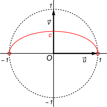
Note that in the above proposition forms a semi-ellipse in the open unit ball obtained by cutting an ellipse in half on the major axis; see Fig.1. In the special case of , the semi-ellipse becomes a straight line.
Next, let us proceed to considering the 2-dimensional case. In searching for 2-dimensional e-autoparallel submanifolds, the previously obtained knowledge of e-geodesics provides an important clue. If a 2-dimensional submanifold is e-autoparallel, it must be e-totally geodesic, and hence the surface should be a union of semi-ellipses. The following proposition claims that a 2-dimensional e-autoparallel submanifold is obtained as a semi-ellipsoid formed by rotating a semi-ellipse representing an e-geodesic around its minor axis.
Proposition 9.2.
Given an orthonormal basis of and a real constant satisfying , let
| (9.17) |
where
| (9.18) |
Then is e-autoparallel in , and the parameter is m-affine as a coordinate system of . More specifically, letting , , and be the e-parallel distribution defined from by (8.6), is an integral manifold of and .
Proof For , let
where and . Noting that
we have
where the terms proportional to included in and cancel, yielding the last line. Owing to (9.9) this implies that the SLDs satisfy for , which means that the first condition in (3.33) is satisfied. The second condition is also satisfied since . Thus the claim of the proposition follows from Prop. 3.8.
As can be seen from naive geometric intuition, for any point in and any plane containing , where is a 2-dimensional linear subspace of , there always exist an orthonormal basis and a constant such that the semi-ellipsoid defined from them by (9.17) and (9.18) contains and has as the tangent plane at . In fact, such and are obtained as follows: take an orthonormal basis so that , and then let (i.e. the squared norm of the orthogonal projection of onto ), , and . Since , this fact means that satisfies condition (i) of Prop. 8.3, and necessarily satisfies condition (ii) as well. Invoking (3.26), condition (ii) is expressed as follows.
Proposition 9.3.
When , for any and any satisfying we have
| (9.19) |
This proposition can also be proved directly by the use of the following lemma, whose proof is given in A5 of Appendix.
Lemma 9.4.
When , for any and any , we have
| (9.20) |
The following proposition immediately follows from Prop. 9.3, which presents a remarkable contrast to Prop. 8.8 for the case .
Proposition 9.5.
When , for any orthonormal basis of it holds that
| (9.22) |
Proof Obvious from Prop. 9.3 since is an -linear space with .
Thus, the distribution is involutive, and induces a foliation whose leaves are 2-dimensional e-autoparallel submanifolds that are integral manifolds of . Furthermore, we can see from the following lemma that every -dimensional e-autoparallel submanifold of is an integral manifold of for some .
Lemma 9.6.
When , for any there exists an orthonormal basis such that .
Proof Let be an orthonormal basis that diagonalizes , and choose so that and . Then satisfies the desired condition.
10 Concluding remarks
In this paper we studied the autoparallelity w.r.t. the e-connection for an information-geometric structure induced on . In particular, we focused on the e-autoparallelity for the SLD structure, for which two different estimation-theoretical characterizations were given. We also investigated the existence conditions for e-autoparallel submanifolds by way of the involutivity of e-parallel distributions and its relation to the torsion tensor. As a result, a specialty of the qubit case was revealed.
Since the obtained estimation-theoretical characterizations of the e-autoparallelity are complete in themselves, we do not see at this time what kind of development lies ahead. It is expected that the future development of quantum estimation theory and related fields may reveal new directions. The classical exponential family has a variety of important properties besides the existence of efficient estimator, some of which may present new materical to characterize certain geometric notions.
For the autoparallelity w.r.t. non-flat connections, our understanding is still very limited. For example, we do not yet have the whole picture about e-autoparallel submanifolds of when . We look forward to further research on this topic in information geometry and/or general differential geometry.
It may also be a challenging problem to develop the infinite-dimensional quantum information geometry so that Theorem 5.1 is extended to the case when and that the naive geometric consideration on the quantum Gaussian shift model presented in Section 6 is mathematically justified.
Geometry of quantum statistical manifolds in an asymptotic framework would also be an important subject to be addressed. For example, consider a sequence , , of i.i.d. extensions of a quantum statistical model . Recent progress in asymptotic quantum statistics has revealed that the sequence exhibits a desirable property called a quantum local asymptotic normality, which tells us that in a shrinking () neighbourhood of a given point , the sequence converges to a quantum Gaussian shift model [12, 13, 14, 15, 16]. As pointed out in Section 6, the limiting quantum Gaussian shift model has a characteristic feature in view of quantum information geometry. It would, therefore, be an interesting future project to extend the geometrical idea presented in this paper to an asymptotic framework so that the convergence of quantum statistical manifolds can be discussed under a suitably chosen topology.
Acknowledgments
This work was partly supported by JSPS KAKENHI Grant Numbers 23H05492 (HN), 23H01090 (AF) and 17H02861 (HN, AF).
References
- [1] Rao CR. Linear Statistical Inference and Its Applications (2nd ed). John Wiley & Sons (1973).
- [2] Kiefer JC. Introduction to Statistical Inference. Springer-Verlag (1987).
- [3] Amari S, Nagaoka H. Methods of Information Geometry. American Mathematical Society, Oxford University Press (2000).
- [4] Kobayashi S, Nomizu K. Foundations of Differential Geometry, II. New York: John Wiley & Sons (1969).
- [5] Nagaoka H., Amari S. Differential geometry of smooth families of probability distributions. METR 82-7, Dept Math Eng and Instr Phys, Univ. of Tokyo (1982). (https://www.keisu.t.u-tokyo.ac.jp/research/techrep/y1982/) (https://bsi-ni.brain.riken.jp/database/item/104)
- [6] Helstrom CW. Minimum mean-square error estimation in quantum statistics. Phys Lett (1967) 25A:101–102 .
- [7] Helstrom CW. Quantum Detection and Estimation Theory. New York: Academic Press (1976).
- [8] Holevo AS. Probabilistic and Statistical Aspects of Quantum Theory. Pisa: Edizioni della Normale (2011). (the previous edition. Amsterdam: North-Holland (1982).)
- [9] Petz D. Monotone metrics on matrix spaces. Linear Algebra Appl (1996) 244:81–96.
- [10] Ohara A. Geodesics for dual connections and means on symmetric cones. Integr equ oper theory (2004) 50:537–548.
- [11] Nagaoka H. Information-geometrical characterization of statistical models which are statistically equivalent to probability simplexes. Proc. 2017 IEEE International Symposium on Information (2017) 1346–1350.
- [12] Guţă M, Kahn J. Local asymptotic normality for qubit states. Phys Rev A (2006) 73:052108.
- [13] Kahn, J, Guţă M. Local asymptotic normality for finite dimensional quantum systems. Comm Math Phys (2009) 289:597–652.
- [14] Yamagata K, Fujiwara A, Gill RD. Quantum local asymptotic normality based on a new quantum likelihood ratio, Ann Statist (2013) 41:2197–2217.
- [15] Fujiwara A, Yamagata K. Noncommutative Lebesgue decomposition and contiguity with application to quantum local asymptotic normality. Bernoulli (2020) 26:2105–2142.
- [16] Fujiwara A, Yamagata K. Efficiency of estimators for locally asymptotically normal quantum statistical models. Ann Statist (to appear). (arXiv:2209.00832)
Appendix
A1 Proof of (3.26)
We first consider the general situation where the e-connection is determined by a family of inner products , and show that the torsion of is represented as follows: for any ,
| (A.1) |
where denotes the derivative of the super-operator-valued map w.r.t. , and denotes tha map . In fact, invoking (3.8) and (3.27), we have for any ,
Noting that
we obtain (A.1). For the SLD structure, we have , which yields that for any point and any tangent vectors ,
Similarly, we have
A2 Proof of Lemma 4.2
- (1)
- (2)
A3 Proofs of Propositions 7.9, 7.10 and 7.11
Proof of Prop. 7.9 This proposition is essentially contained in Theorem 7.2 of [3]. Here we give a proof for the reader’s convenience.
Given and , there exists a tangent vector satisfying by (3.10). Applying (7.18) to the case , we have , and hence
A4 A result on the relationship between autoparallelity and total geodesicness
In Remark 8.6 we noted that condition (ii) of Prop. 8.3 implies the equivalence between autoparallelity and total geodesicness. This is restated in the following proposition.
Proposition A.1.
Suppose that an affine connection is given on a manifold whose torsion satisfies
| (A.8) |
Then every -totally geodesic submanifold of is -autoparallel.
We present a proof below, which is almost parallel to the proof of Theorem 8.4 in Chap. VII of [4] cited as a result due to E. Cartan.
Proof Let , and be a -totally geodesic submanifold with . We take a coordinate system of such that is represented as
and that forms a coordinate system of . Let , , and denote the connection coefficients of w.r.t. by : for . For arbitrary , it follows from the assumption (A.8) that , which implies that for any . Hence we have
| (A.9) |
Given a point and a tangent vector arbitrarily, let be a -geodesic with an affine parameter satisfying and . The geodesic should satisfy the differential equation , which is represented as
Since is assumed to be -totally geodesic, stays in and hence for . Therefore, the above equation yields
and letting , we obtain
Since and are arbitrary and is symmetric w.r.t. by (A.9), it follows that
| (A.10) |
Now, for arbitrary vector fields and on , where , we have
which concludes that is -autoparallel in .