This paper was converted on www.awesomepapers.org from LaTeX by an anonymous user.
Want to know more? Visit the Converter page.

Axion-meson mixing in light of recent lattice η\eta-η\eta^{\prime} simulations and their two-photon couplings within U(3)U(3) chiral theory

Rui Gaoa,  Zhi-Hui Guoa,b111 zhguo@hebtu.edu.cn,   J. A. Ollerc222 oller@um.es,  Hai-Qing Zhoud333 zhouhq@seu.edu.cn
a Department of Physics and Hebei Key Laboratory of Photophysics Research and Application,
Hebei Normal University, Shijiazhuang 050024, China
b CAS Key Laboratory of Theoretical Physics, Institute of Theoretical Physics,
Chinese Academy of Sciences, Beijing 100190, China
c Departamento de Física. Campus de Espinardo, Murcia E-30071, Spain
d School of Physics, Southeast University, Nanjing 211189, China
Abstract

We study the mixing of the QCD/QCD-like axion and light-flavor mesons π0,η,η\pi^{0},\eta,\eta^{\prime} within the framework of U(3)U(3) chiral perturbation theory up to next-to-leading order in this work. The axion-meson mixing formulas are calculated order by order in the U(3)U(3) δ\delta-expansion scheme, namely the joint expansions of the momentum, light-quark masses and 1/NC1/N_{C}. We provide axion-meson mixing relations in terms of the π0\pi^{0}-η\eta-η\eta^{\prime} mixing parameters and their masses. The recent lattice simulations on the η\eta-η\eta^{\prime} systems turn out to be able to offer valuable inputs to constrain the unknown low-energy constants. The relation of the mass and decay constant of the axion is then further explored based on our updated calculations. The two-photon couplings of the light-flavor mesons, together with the axion, are also investigated in the U(3)U(3) chiral theory up to next-to-leading order in the δ\delta-counting scheme.

1 Introduction

The hypothetical particle axion provides an elegant solution to the long standing strong CP problem [1, 2, 3]. Since its first proposal in late 1970s, tremendous efforts have been put in various fields of physics to search this intriguing hypothesized particle, ranging from particle physics, astronomy, cosmology to condensed matter and optical physics, etc [4].

In the Peccei-Quinn (PQ) picture, axion corresponds to the pseudo-Nambu-Goldstone boson (pNGB) resulting from the breaking of the global UPQ(1)U_{\rm PQ}(1) symmetry. In the low-energy regime, the most characteristic interaction of the axion is the coupling with the topological gluon density, i.e., a/faGμνG~μνa/f_{a}\,G^{\mu\nu}\tilde{G}_{\mu\nu}, where GμνG^{\mu\nu} is the gluon field strength tensor, its dual is G~μν=εμνρσGρσ/2\tilde{G}_{\mu\nu}=\varepsilon_{\mu\nu\rho\sigma}G^{\rho\sigma}/2 with εμνρσ\varepsilon_{\mu\nu\rho\sigma} the Levi-Civita antisymmetric tensor and faf_{a} stands for the axion decay constant. The essential point of the PQ mechanism to solve the strong CP problem relies on the cancellation of the CP violating term θGμνG~μν\theta G^{\mu\nu}\tilde{G}_{\mu\nu} in QCD by the dynamical generation of a proper vacuum expectation value (VEV) from the axion field. Different ultraviolet (UV) models in the new physics sector can lead to rather different couplings of the axion with other standard-model (SM) particles, such as the leptons, quarks, photon and W/Z bosons [2, 3, 5, 6, 7, 8], although they can be constructed to give a universal GG~G\tilde{G} coupling.

Due to the nonperturbative nature of the gluons in the low-energy region, the common way to study the interactions of the axion is to first perform the axial transformation of the quark fields to eliminate the a/faGμνG~μνa/f_{a}\,G^{\mu\nu}\tilde{G}_{\mu\nu} operator from the beginning and then match to the axion chiral perturbation theory (χ\chiPT), which encodes the axion field together with the pions in the SU(2)SU(2) case, and the octet of π,K,η8\pi,K,\eta_{8} in the SU(3)SU(3) case. On the other hand, it is also possible to directly match the anomalous axion term a/faGμνG~μνa/f_{a}\,G^{\mu\nu}\tilde{G}_{\mu\nu} with the operators. In this regard, it is reminded that the large mass of the singlet pseudoscalar η0\eta_{0} (the dominant component of the physical η\eta^{\prime} meson), compared to those of the pseudoscalar octet π,K\pi,K and η8\eta_{8}, can be mainly attributed to the anomalous breaking of the QCD UA(1)U_{A}(1) symmetry. Therefore, it implies that another way to introduce the axion field into χ\chiPT can be similar to the case of the singlet η0\eta_{0}. The pioneer work to study the influence of the η\eta^{\prime} on the axion properties can trace back to Refs. [9, 10]. Recently many works aiming at the extended descriptions of the axion-η()\eta^{(^{\prime})} interactions are proposed from different points of view [11, 12, 13, 14, 15, 16, 17, 18, 19, 20], including the axion production from the η/η\eta/\eta^{\prime} and kaon decays, CP violating axion signals, the axion-baryon couplings, the model-independent part of the axion-photon-photon coupling, etc. In this work, we will further pursue a systematical calculation of the axion-ϕ\phi (ϕ=π,η,η\phi=\pi,\eta,\eta^{\prime}) interactions order by order within the U(3)U(3) by employing the δ\delta expansion scheme [21, 22, 23], namely, a simultaneous expansion in powers of the momenta, light-quark masses and 1/NC1/N_{C}, i.e. δp2mq1/NC\delta\sim p^{2}\sim m_{q}\sim 1/N_{C}. In addition, we also study the relations of the model-independent two-photon couplings of the axion, together with those of the π0,η\pi^{0},\eta and η\eta^{\prime} mesons, by performing the next-to-leading order (NLO) U(3)U(3) calculations.

The layout of this paper is as follows. The relevant chiral Lagrangians up to NLO are elaborated in Sec. 2. We address the mixing formalism at leading order (LO) for the four-particle system involving π0,η,η\pi^{0},\eta,\eta^{\prime} and the axion in Sec. 3. The calculation of the NLO mixing, the fits to relevant lattice data and numerical analyses of the transitions matrix elements, and the masses of π0,η,η\pi^{0},\eta,\eta^{\prime} and the axion are given in Sec. 4. The two-photon couplings of the aforementioned four particles are then studied up to NLO in the U(3)U(3) χ\chiPT in Sec. 5. A short summary and conclusions are given in Sec. 6.

2 Axion U(3)U(3) up to next-to-leading order

The axion is characterized by the interaction with the gluons and its effective operators can be written as

aG=12μaμa+afaαs8πi=18GμνiG~i,μν12ma,02a2,\displaystyle\mathcal{L}_{a}^{G}=\frac{1}{2}\partial_{\mu}a\partial^{\mu}a+\frac{a}{f_{a}}\frac{\alpha_{s}}{8\pi}\sum_{i=1}^{8}G^{i}_{\mu\nu}\tilde{G}^{i,\mu\nu}-\frac{1}{2}m_{a,0}^{2}\,a^{2}\,, (1)

where GμνiG^{i}_{\mu\nu} and G~μνi\tilde{G}^{i}_{\mu\nu} are the gluon field strength tensor and its dual, with ii the color indices. The second term in Eq. (1) is considered to be model-independent, due to its relevance of solving the strong CP problem. For the bare mass ma,0m_{a,0} of the axion in the third term, its value is usually assumed to be vanishing in the minimal QCD axion setup [1, 2, 3], although it is also possible to have a nonvanishing ma,0m_{a,0} to solve the strong CP problem [24, 25, 26, 27, 4]. The direct couplings of the axion with the photon and fermions heavily rely on the specific model-building considerations in the BSM sector. In this work, we focus on the axion interactions with the hadrons and photon that are purely induced by the effective Lagrangian in Eq. (1), i.e. the model-independent parts of the axion-hadron and axion-photon interactions.

The next step is to match the effective Lagrangian in Eq. (1) to the axion chiral perturbation theory [28, 29], which provides a reliable framework to study the axion-hadron interactions order by order. In the low-energy QCD, apart from the chiral symmetry breaking, another distinct feature is the QCD UA(1)U_{A}(1) anomaly, i.e. the anomalous breaking of the UA(1)U_{A}(1) symmetry by topological charge density ω(x)=αsGμνG~μν/(8π)\omega(x)=\alpha_{s}G_{\mu\nu}\tilde{G}^{\mu\nu}/(8\pi), which gives a natural explanation of the large mass of the singlet η0\eta_{0} even in the chiral limit. In this work we will carry out the study sticking to the U(3)U(3) by employing the large NCN_{C} argument [30]. This implies that one can explicitly include the axion field into the Lagrangian in a similar way as the situation of the η\eta^{\prime}. To be more specific, we use the δ\delta-expansion scheme to arrange the various contributions in U(3)U(3) by simultaneously considering the expansions in the momenta, light-quark masses and 1/NC1/N_{C} [22, 23, 21].

To set up the notations, we briefly recapitulate the way to construct the LO operators of U(3)U(3) . From the large NCN_{C} point of view, the singlet η0\eta_{0} would become the ninth pNGB in the large NCN_{C} and chiral limits, since the instanton effect via the QCD UA(1)U_{A}(1) anomaly is 1/NC1/N_{C} suppressed. Then, the dynamical fields in low energy QCD form the pNGB nonet, which is usually parameterized as U=exp(i2Φ/F)U={\exp}\big{(}i\sqrt{2}\Phi/F\big{)}, with the pNGB nonet matrix given by

Φ=(12π0+16η8+13η0π+K+π12π0+16η8+13η0K0KK¯026η8+13η0).\Phi\,=\,\left(\begin{array}[]{ccc}\frac{1}{\sqrt{2}}\pi^{0}+\frac{1}{\sqrt{6}}\eta_{8}+\frac{1}{\sqrt{3}}\eta_{0}&\pi^{+}&K^{+}\\ \pi^{-}&\frac{-1}{\sqrt{2}}\pi^{0}+\frac{1}{\sqrt{6}}\eta_{8}+\frac{1}{\sqrt{3}}\eta_{0}&K^{0}\\ K^{-}&\overline{K}^{0}&\frac{-2}{\sqrt{6}}\eta_{8}+\frac{1}{\sqrt{3}}\eta_{0}\end{array}\right)\,. (2)

The QCD UA(1)U_{A}(1) anomaly effect can be incorporated in effective Lagrangian via the operator τ2(ilogdetU)2-\frac{\tau}{2}(-i\log\det U)^{2}, where τ\tau corresponds to the topological susceptibility [23]. Taking into account that detU=exp(TrlogU)\det U=\exp({\rm Tr}\log U), the former operator can be cast as 3τη02/F2-3\tau\eta_{0}^{2}/{F^{2}}, which is nothing but the mass term for singlet η0\eta_{0} in the chiral limit. In practice it is convenient to introduce M02=6τF2M_{0}^{2}=\frac{6\tau}{F^{2}} as the LO mass squared for η0\eta_{0}. In the large NCN_{C} counting rule, the topological susceptibility τ\tau and the pNGB decay constant FF scale like O(1)O(1) and O(NC)O(\sqrt{N_{C}}), respectively [23, 31], which indicate that M02M_{0}^{2} behaves as O(1/NC)O(1/N_{C}). Under the PQ assumption, the CP violating θGG~\theta G\tilde{G} term is canceled by the VEV part of the axion via the aGG~aG\tilde{G} term in Eq. (1). Therefore, this indicates that the anomalous aGG~aG\tilde{G} effect can be included in the chiral effective Lagrangian in a similar fashion as the θ\theta term, the latter of which is discussed in great detail in Ref. [23]. According to the recipe in the previous reference, the axion field can be introduced to the LO U(3)U(3) together with the anomalous mass for η0\eta_{0} via τ2(ilogdetU+a/fa)2=τ2(6η0/F+a/fa)2-\frac{\tau}{2}(-i\log\det U+a/f_{a})^{2}=-\frac{\tau}{2}(\sqrt{6}\eta_{0}/F+a/f_{a})^{2}. For phenomenological convenience, we will always use the parameter M0M_{0} to replace the topological susceptibility τ\tau in the following discussions. On general grounds, the axion chiral transformation on the quark fields needed to remove the aGG~aG\tilde{G} term in Eq. (1) is of the same type as the singlet axial chiral transformation UA(1)U_{A}(1) that is parameterized as exp(iη02/3)\exp(i\eta_{0}\sqrt{2/3}). This observation drives to the necessity of adding together the fields of the axion and η0\eta_{0} in the large NCN_{C} and chiral limit, where the latter is a pNGB of QCD parameterized as coordinates in the coset space UL(3)UR(3)/UV(3)U_{L}(3)\otimes U_{R}(3)/U_{V}(3) [32]. Under these circumstances, the LO U(3)U(3) including the axion field takes the form

LO=F24uμuμ+F24χ++F212M02X2,\displaystyle\mathcal{L}^{\rm LO}=\frac{F^{2}}{4}\langle u_{\mu}u^{\mu}\rangle+\frac{F^{2}}{4}\langle\chi_{+}\rangle+\frac{F^{2}}{12}M_{0}^{2}X^{2}\,, (3)

where the axion field is introduced via

X=log(detU)+iafa,\displaystyle X=\log{(\det U)}+i\frac{a}{f_{a}}\,, (4)

and other basic building blocks are given by

U=u2=ei2ΦF,χ=2B(s+ip),χ±=uχu±uχu,\displaystyle U=u^{2}=e^{i\frac{\sqrt{2}\Phi}{F}}\,,\qquad\chi=2B(s+ip)\,,\qquad\chi_{\pm}=u^{\dagger}\chi u^{\dagger}\pm u\chi^{\dagger}u\,,
uμ=iuDμUu,DμU=μUi(vμ+aμ)U+iU(vμaμ).\displaystyle u_{\mu}=iu^{\dagger}D_{\mu}Uu^{\dagger}\,,\qquad D_{\mu}U\,=\,\partial_{\mu}U-i(v_{\mu}+a_{\mu})U\,+iU(v_{\mu}-a_{\mu})\,. (5)

Here, ss, pp, vμv_{\mu}, and aμa_{\mu} are external scalar, pseudoscalar, vector and axial-vector external sources, respectively, introduced as spurion fields. The quark-mass corrections are introduced by fixing s=Mqdiag(mu,md,ms)s=M_{q}\equiv{\rm diag}(m_{u},m_{d},m_{s}). The parameter M0M_{0} in the last term of Eq. (3) corresponds to the leading-order mass of the η0\eta_{0}, which squared is proportional to the topological susceptibility [23]. The leading scaling behavior of M02M_{0}^{2} is O(1/NC)O(1/N_{C}) in the δ\delta-counting scheme [30].

Another approach frequently used in literature to introduce the axion field in , e.g. as those in Refs. [28, 29], is to first perform the axial transformation of the quark fields to eliminate the axion-gluon operator in Eq. (1), i.e., by taking

qeia2faγ5Qaq,[q=(u,d,s)T],\displaystyle q\to e^{i\frac{a}{2f_{a}}\gamma_{5}Q_{a}}q\,,\qquad[q=(u,d,s)^{\rm T}]\,, (6)

where QaQ_{a} is a 3×33\times 3 matrix spanned in the light three-flavor space. Such a transformation induces two additional terms in the effective Lagrangian (1): aαs8πfaGμνG~μνTr(Qa)-\frac{a\alpha_{s}}{8\pi f_{a}}G_{\mu\nu}\tilde{G}^{\mu\nu}\,{\rm Tr}(Q_{a}) and μa2faq¯γμγ5Qaq-\frac{\partial_{\mu}a}{2f_{a}}\bar{q}\gamma^{\mu}\gamma_{5}Q_{a}q. The former term exactly cancels the axion-gluon operator in Eq. (1), after taking the constraint Tr(Qa)=1{\rm Tr}(Q_{a})=1. While, the latter term describes the extra axion-quark interaction that is induced by the axial transformation (6). In addition, it is easy to demonstrate that this transformation will also introduce the axion field into the quark masses: MqMq(a)=eia2faQaMqeia2faQaM_{q}\to M_{q}(a)=e^{i\frac{a}{2f_{a}}Q_{a}}M_{q}e^{i\frac{a}{2f_{a}}Q_{a}}, which can lead to non-derivative axion interactions. In the SU(3)SU(3) χ\chiPT, the LO mass mixing between the axion and the neutral unflavored π0\pi^{0} and η8\eta_{8} can be avoided by taking QaMq1Q_{a}\propto M_{q}^{-1}. However, in the U(3)U(3) case, even if one imposes the latter form for QaQ_{a}, the mixing between the axion and the singlet η0\eta_{0} still exists at LO. Therefore, in this work we will not perform the transformation of quark fields (6), and use instead the original U(3)U(3) Lagrangian in Eq. (3) to proceed the calculations. The physical results should be the same regardless of keeping the aGG~aG\tilde{G} term or replacing it via the axial transformation (6), although the intermediate steps in the calculations can look different.

In the rest of the discussions, we will stick to the method by including the axion in the U(3)U(3) through the XX field of Eq. (4). In this case, the axion U(3)U(3) Lagrangian coincides with the standard one with the obvious replacement of the XX field. When restricting to the axion-meson mixing, the relevant NLO Lagrangian under the δ\delta-counting rule consists of four operators

NLO=L5uμuμχ++L82χ+χ++χχF2Λ112DμXDμXF2Λ212Xχ,\displaystyle\mathcal{L}^{\rm NLO}=L_{5}\langle u^{\mu}u_{\mu}\chi_{+}\rangle+\frac{L_{8}}{2}\langle\chi_{+}\chi_{+}+\chi_{-}\chi_{-}\rangle-\frac{F^{2}\,\Lambda_{1}}{12}D^{\mu}XD_{\mu}X-\frac{F^{2}\,\Lambda_{2}}{12}X\langle\chi_{-}\rangle\,, (7)

where the first two terms accompanied by L5L_{5} and L8L_{8} share the same forms as those from the conventional SU(3)SU(3)  [31]. Within the framework of , the NCN_{C} order of a given operator can be inferred by the number of traces in the flavor space [31]. Generally speaking, one extra trace will bring one additional 1/NC1/N_{C} suppression order to the effective operator. By taking into account the identity of logdetU=logU\log\det U=\langle\log U\rangle, it is straightforward to conclude that the first two terms in Eq. (7) are counted as O(p4,NC)O(p^{4},N_{C}), and the remaining two terms with Λ1\Lambda_{1} and Λ2\Lambda_{2} that only appear in the U(3)U(3) case [23] are counted as O(p2,NC0)O(p^{2},N_{C}^{0}).

The two-photon decays of the light pseudoscalar mesons are governed by the Wess-Zumino-Witten Lagrangian and the relevant LO Lagrangian [33, 34] is

WZWLO=32e28π2FεμνρσμAνρAσQ2Φ,\displaystyle\mathcal{L}_{WZW}^{\rm LO}=-\frac{3\sqrt{2}e^{2}}{8\pi^{2}F}\varepsilon_{\mu\nu\rho\sigma}\partial^{\mu}A^{\nu}\partial^{\rho}A^{\sigma}\langle Q^{2}\Phi\rangle\,, (8)

which is counted as O(p4,NC)O(p^{4},N_{C}) in the δ\delta-counting scheme. The quantity QQ stands for the matrix of the electric charges of the light quarks, i.e. Q=Diag(2e3,e3,e3)Q={\rm Diag}(\frac{2e}{3},-\frac{e}{3},-\frac{e}{3}), with ee the magnitude of the electron charge, and AμA_{\mu} stands for the photon field. At NLO there are two additional terms [35, 36]

WZWNLO=it1εμνρσf+μνf+ρσχ+k3εμνρσf+μνf+ρσX,\displaystyle\mathcal{L}_{WZW}^{\rm NLO}=it_{1}\varepsilon_{\mu\nu\rho\sigma}\langle f_{+}^{\mu\nu}f_{+}^{\rho\sigma}\chi_{-}\rangle+k_{3}\varepsilon_{\mu\nu\rho\sigma}\langle f_{+}^{\mu\nu}f_{+}^{\rho\sigma}\rangle X\,, (9)

with

f+μν=uFLμνu+uFRμνu,\displaystyle f_{+}^{\mu\nu}=uF_{L}^{\mu\nu}u^{\dagger}+u^{\dagger}F_{R}^{\mu\nu}u\,, (10)

where FLμν=μFLνμFLνi[FLμ,FLν]F_{L}^{\mu\nu}=\partial^{\mu}F_{L}^{\nu}-\partial^{\mu}F_{L}^{\nu}-i[F_{L}^{\mu},F_{L}^{\nu}] and FRμν=μFRνμFRνi[FRμ,FRν]F_{R}^{\mu\nu}=\partial^{\mu}F_{R}^{\nu}-\partial^{\mu}F_{R}^{\nu}-i[F_{R}^{\mu},F_{R}^{\nu}], with FLμ=vμaμF_{L}^{\mu}=v^{\mu}-a^{\mu} and FRμ=vμ+aμF_{R}^{\mu}=v^{\mu}+a^{\mu}, denote the field strength tensors of left-hand and right-hand external sources, respectively. One can take FLμF_{L}^{\mu}=FRμF_{R}^{\mu}= eQAμ-eQA^{\mu} to obtain the interaction vertexes with photons. The t1t_{1} and k3k_{3} terms in Eq. (9) belong to the O(p6,NC)O(p^{6},N_{C}) and O(p4,NC0)O(p^{4},N_{C}^{0}) types of operators in the δ\delta counting, respectively. When restricting to the pseudoscalar-photon-photon case, the Lagrangian (9) reduces to

WZWNLO=\displaystyle\mathcal{L}_{WZW}^{\rm NLO}= t1322BFεμνρσμAνρAσ(MqΦ+ΦMq)Q2\displaystyle t_{1}\frac{32\sqrt{2}B}{F}\varepsilon_{\mu\nu\rho\sigma}\partial^{\mu}A^{\nu}\partial^{\rho}A^{\sigma}\langle\big{(}M_{q}\Phi+\Phi M_{q}\big{)}Q^{2}\rangle
+16k3εμνρσμAνρAσQ2(2FΦ+afa).\displaystyle+16k_{3}\varepsilon_{\mu\nu\rho\sigma}\partial^{\mu}A^{\nu}\partial^{\rho}A^{\sigma}\langle Q^{2}\rangle\bigg{(}\frac{\sqrt{2}}{F}\langle\Phi\rangle+\frac{a}{f_{a}}\bigg{)}\,. (11)

According to the Lagrangians in Eqs. (3) and (8), the LO interactions of the axion with the pNGBs and photons are purely caused by the mixing of the axion and the neutral unflavored pNGBs. Therefore it is mandatory to first address the axion-pNGBs mixing problem.

3 Revisiting the mixing formalism at LO

In principle, there are both kinetic and mass mixings between different states [37, 38]. At LO in the δ\delta counting, the π0,η,η\pi^{0},\eta,\eta^{\prime} and aa will get mixing purely via the mass terms from the Lagrangian (3), while the kinetic mixing only starts to appear in the NLO Lagrangian (7). We calculate the mixing of the axion and π0,η,η\pi^{0},\eta,\eta^{\prime} order by order below.

In Refs. [39, 40, 41, 42], the η\eta-η\eta^{\prime} mixing has been studied up to next-to-next-to leading order in the δ\delta expansion in the isospin limit. As first pointed out in Ref. [39], it is convenient to use the η¯̊\mathring{\overline{\eta}} and η¯̊\mathring{\overline{\eta}}^{\prime} that are diagonalized at LO, if one attempts to perform a systematical higher-order calculation in the U(3)U(3) chiral theory relying on the δ\delta counting. The key reason is that the LO mixing vertex of the η8\eta_{8} and η0\eta_{0} is formally counted as the same order of their LO masses, implying that an infinity insertion of the LO mixing vertex of η0\eta_{0} and η8\eta_{8} in the loop calculations will not get suppressed in the δ\delta-counting scheme, see Fig. 1 of Ref. [39] for illustrations. This cumbersome problem can be avoided by first performing the LO diagonalization of η8\eta_{8} and η0\eta_{0} and using the LO diagonalized fields η¯̊\mathring{\overline{\eta}} and η¯̊\mathring{\overline{\eta}}^{\prime}, whose relations are given by

(η¯̊η¯̊)=(cθsθsθcθ)(η8η0),\displaystyle\left(\begin{array}[]{c}\mathring{\overline{\eta}}\\ \mathring{\overline{\eta}}^{\prime}\end{array}\right)=\left(\begin{array}[]{cc}c_{\theta}&-s_{\theta}\\ s_{\theta}&c_{\theta}\end{array}\right)\left(\begin{array}[]{c}\eta_{8}\\ \eta_{0}\end{array}\right)\,, (18)

with cθ=cosθc_{\theta}=\cos{\theta} and sθ=sinθs_{\theta}=\sin{\theta}. The reason behind is that the mixing strengths between η¯̊\mathring{\overline{\eta}} and η¯̊\mathring{\overline{\eta}}^{\prime} are suppressed at least by one higher order in the δ\delta-counting rule. From the Lagrangian (3), the LO mixing angle θ\theta and masses of η¯̊\mathring{\overline{\eta}} and η¯̊\mathring{\overline{\eta}}^{\prime} can be calculated

mη¯2\displaystyle m_{\overline{\eta}}^{2} =\displaystyle= M022+mK¯2M044M02Δ23+4Δ42,\displaystyle\frac{M_{0}^{2}}{2}+m_{\overline{K}}^{2}-\frac{\sqrt{M_{0}^{4}-\frac{4M_{0}^{2}\Delta^{2}}{3}+4\Delta^{4}}}{2}\,, (19)
mη¯2\displaystyle m_{\overline{\eta}^{\prime}}^{2} =\displaystyle= M022+mK¯2+M044M02Δ23+4Δ42,\displaystyle\frac{M_{0}^{2}}{2}+m_{\overline{K}}^{2}+\frac{\sqrt{M_{0}^{4}-\frac{4M_{0}^{2}\Delta^{2}}{3}+4\Delta^{4}}}{2}\,, (20)
sinθ\displaystyle\sin{\theta} =\displaystyle= (1+(3M022Δ2+9M0412M02Δ2+36Δ4)232Δ4)1,\displaystyle-\left(\sqrt{1+\frac{\big{(}3M_{0}^{2}-2\Delta^{2}+\sqrt{9M_{0}^{4}-12M_{0}^{2}\Delta^{2}+36\Delta^{4}}\big{)}^{2}}{32\Delta^{4}}}~{}\right)^{-1}\,, (21)

where Δ2=mK¯2mπ¯2\Delta^{2}=m_{\overline{K}}^{2}-m_{\overline{\pi}}^{2}, and mπ¯m_{\overline{\pi}} and mK¯m_{\overline{K}} are the LO masses of the pion and kaon in the isospin symmetric limit, respectively.

New subtle complexities will arise when simultaneously including the π0\pi^{0}, the axion aa, η\eta and η\eta^{\prime}. On one hand, the isospin breaking (IB) contributions can not be ignored any more, since the mixings between the π0\pi^{0} and the remaining fields η\eta, η\eta^{\prime} and aa are caused by the IB effects. It is noted that we only consider the IB effects arising from the strong interaction, namely the mass difference between the up and down quarks. On the other hand, the mixings between the axion aa and other fields π0\pi^{0}, η\eta and η\eta^{\prime} are suppressed by the factor F/faF/f_{a}. Additional power counting rules will be introduced to simplify the discussions, apart from the conventional δ\delta-counting that is widely employed in the η\eta-η\eta^{\prime} case. Generally speaking, the magnitudes of the IB corrections are around 12%1\sim 2\%. Compared to the correction in the δ\delta counting, which can be naively estimated to be around 30%30\% [1/(NC=3)1/(N_{C}=3)], it is justified to just keep the leading nonvanishing IB terms. The magnitude of the axion-related suppression factor F/faF/f_{a} is definitely much more smaller than that of the IB corrections. Therefore, at the current stage, it is safe to just take the leading F/faF/f_{a} terms. More precisely, we aim at the systematical calculations of the higher-order corrections in the δ\delta-counting scheme by keeping the leading IB and F/faF/f_{a} terms in this work.

Similarly as the η\eta-η\eta^{\prime} case, it is much more convenient to use the fields π¯0\overline{\pi}^{0}, η¯\overline{\eta}, η¯\overline{\eta}^{\prime} and a¯\overline{a} that already diagonalize LO mass term to systematically calculate the higher-order corrections. Notice that we have used η¯̊\mathring{\overline{\eta}} and η¯̊\mathring{\overline{\eta}}^{\prime} to denote the LO diagonalized η\eta and η\eta^{\prime} fields in the isospin symmetric case, while η¯\overline{\eta} and η¯\overline{\eta}^{\prime} stand for the fields after including the IB effects. As stated before, the leading terms in the IB and F/faF/f_{a} expansions will be kept in our calculation and, in this case, one can obtain the diagonalized states π¯0\overline{\pi}^{0}, η¯\overline{\eta}, η¯\overline{\eta}^{\prime} and a¯\overline{a} by performing the following field redefinitions

(π¯0η¯η¯a¯)=(1+O(v2)v12v13v14v121+O(v2)v23v24v13v231+O(v2)v34v14v24v341+O(v2))(π0η¯̊η¯̊a),\left(\begin{array}[]{c}\overline{\pi}^{0}\\ \overline{\eta}\\ \overline{\eta}^{\prime}\\ \overline{a}\end{array}\right)\,=\,\left(\begin{array}[]{cccc}1+O(v^{2})&-v_{12}&-v_{13}&-v_{14}\\ v_{12}&1+O(v^{2})&-v_{23}&-v_{24}\\ v_{13}&v_{23}&1+O(v^{2})&-v_{34}\\ v_{14}&v_{24}&v_{34}&1+O(v^{2})\end{array}\right)\,\left(\begin{array}[]{c}\pi^{0}\\ \mathring{\overline{\eta}}\\ \mathring{\overline{\eta}}^{\prime}\\ a\end{array}\right)\,, (22)

where π0\pi^{0} and aa correspond to the bare states entering in the Lagrangian (3). The matrix elements vijv_{ij} are determined by the mass mixing terms from the LO Lagrangian (3), and their explicit expressions are found to be

v12=\displaystyle v_{12}= ϵ3cθ2sθmπ¯2mη¯2,\displaystyle-\frac{\epsilon}{\sqrt{3}}\frac{c_{\theta}-\sqrt{2}s_{\theta}}{m_{\overline{\pi}}^{2}-m_{\overline{\eta}}^{2}}\,, (23)
v13=\displaystyle v_{13}= ϵ32cθ+sθmπ¯2mη¯2,\displaystyle-\frac{\epsilon}{\sqrt{3}}\frac{\sqrt{2}c_{\theta}+s_{\theta}}{m_{\overline{\pi}}^{2}-m_{\overline{\eta}^{\prime}}^{2}}\,, (24)
v14=\displaystyle v_{14}= M02ϵ32(ma,02mπ¯2)Ffa[sθ(cθ2sθ)(ma,02+mπ¯2mη¯2)(ma,02mη¯2)(mη¯2mπ¯2)cθ(2cθ+sθ)(ma,02+mπ¯2mη¯2)(ma,02mη¯2)(mη¯2mπ¯2)],\displaystyle\frac{M_{0}^{2}\epsilon}{3\sqrt{2}(m_{a,0}^{2}-m_{\overline{\pi}}^{2})}\frac{F}{f_{a}}\bigg{[}\frac{s_{\theta}(c_{\theta}-\sqrt{2}s_{\theta})(m_{a,0}^{2}+m_{\overline{\pi}}^{2}-m_{\overline{\eta}}^{2})}{(m_{a,0}^{2}-m_{\overline{\eta}}^{2})(m_{\overline{\eta}}^{2}-m_{\overline{\pi}}^{2})}-\frac{c_{\theta}(\sqrt{2}c_{\theta}+s_{\theta})(m_{a,0}^{2}+m_{\overline{\pi}}^{2}-m_{\overline{\eta}^{\prime}}^{2})}{(m_{a,0}^{2}-m_{\overline{\eta}^{\prime}}^{2})(m_{\overline{\eta}^{\prime}}^{2}-m_{\overline{\pi}}^{2})}\bigg{]}\,,
v24=\displaystyle v_{24}= M02sθ6(ma,02mη¯2)Ffa,\displaystyle-\frac{M_{0}^{2}s_{\theta}}{\sqrt{6}(m_{a,0}^{2}-m_{\overline{\eta}}^{2})}\frac{F}{f_{a}}\,, (26)
v34=\displaystyle v_{34}= M02cθ6(ma,02mη¯2)Ffa,\displaystyle\frac{M_{0}^{2}c_{\theta}}{\sqrt{6}(m_{a,0}^{2}-m_{\overline{\eta}^{\prime}}^{2})}\frac{F}{f_{a}}\,, (27)

where mπ¯m_{\overline{\pi}}, mη¯m_{\overline{\eta}} and mη¯m_{\overline{\eta}^{\prime}} correspond to the LO masses of the π\pi, η\eta and η\eta^{\prime} mesons, and ϵ=B(mumd)\epsilon=B(m_{u}-m_{d}) corresponds to the leading strong IB factor. Regarding the matrix element v23v_{23} in Eq. (22), it describes the IB contribution to the η\eta-η\eta^{\prime} mixing, which is expected to play negligible roles comparing with the SU(3)SU(3) symmetry breaking effects. Therefore in this work we will neglect the IB contributions to the η\eta-η\eta^{\prime} mixing, i.e., v23v_{23} will be set to zero throughout. At the LO electromagnetic (EM) correction, the Dashen’s theorem tells us that the EM corrections to the kaon masses equal to the mass differences of the pions [43, 36], i.e. (mK+2mK02)EM=mπ+2mπ02(m_{K^{+}}^{2}-m_{K^{0}}^{2})_{\rm EM}=m_{\pi^{+}}^{2}-m_{\pi^{0}}^{2}, and at this order one can write ϵB(mumd)=mK+2mK02(mπ+2mπ02)\epsilon\equiv B(m_{u}-m_{d})=m_{K^{+}}^{2}-m_{K^{0}}^{2}-(m_{\pi^{+}}^{2}-m_{\pi^{0}}^{2}).

After the diagonalization at LO, the mass of the axion field a¯\overline{a} is found to be

ma¯2=ma,02+M02F26fa2[1+cθ2M02(2ma,02mη¯2)(ma,02mη¯2)2+sθ2M02(2ma,02mη¯2)(ma,02mη¯2)2]+O(ϵ),\displaystyle m_{\overline{a}}^{2}=m_{a,0}^{2}+\frac{M_{0}^{2}F^{2}}{6f_{a}^{2}}\bigg{[}1+\frac{c_{\theta}^{2}M_{0}^{2}(2m_{a,0}^{2}-m_{\overline{\eta}^{\prime}}^{2})}{(m_{a,0}^{2}-m_{\overline{\eta}^{\prime}}^{2})^{2}}+\frac{s_{\theta}^{2}M_{0}^{2}(2m_{a,0}^{2}-m_{\overline{\eta}}^{2})}{(m_{a,0}^{2}-m_{\overline{\eta}}^{2})^{2}}\bigg{]}+O(\epsilon)\,, (28)

which by taking ma,0=0m_{a,0}=0 reduces to the minimal setup of the QCD axion case

ma¯2=M02F26fa2[1cθ2M02mη¯2sθ2M02mη¯2]+O(ϵ).\displaystyle m_{\overline{a}}^{2}=\frac{M_{0}^{2}F^{2}}{6f_{a}^{2}}\bigg{[}1-\frac{c_{\theta}^{2}M_{0}^{2}}{m_{\overline{\eta}^{\prime}}^{2}}-\frac{s_{\theta}^{2}M_{0}^{2}}{m_{\overline{\eta}}^{2}}\bigg{]}+O(\epsilon)\,. (29)

It should be stressed that the neat analytical expressions in Eqs. (23)-(29) are obtained by keeping the leading IB effects in π0\pi^{0}-aa and π0η()\pi^{0}-\eta^{(^{\prime})} mixing and neglecting the IB contributions to the aa-η()\eta^{(^{\prime})} mixing and the masses of the axion and pNGBs. The concise formulas in Eqs. (28) and (29) give us direct access to estimate the influences from the pertinent η\eta-η\eta^{\prime} mixing parameters to the axion mass in different scenarios. We take the minimal QCD axion case, i.e. Eq. (29), to carry out some exploratory phenomenological discussions.

By taking the LO expressions of the η\eta-η\eta^{\prime} mixing in Eqs. (19), (20) and (21), it is easy to demonstrate that the axion mass squared can be recast as

ma¯2=F2fa2M02mπ¯2(2mK¯2mπ¯2)8M02mK¯22mπ¯2(M026mK¯2)6mπ¯4,\displaystyle m_{\overline{a}}^{2}=\frac{F^{2}}{f_{a}^{2}}\frac{M_{0}^{2}m_{\overline{\pi}}^{2}(2m_{\overline{K}}^{2}-m_{\overline{\pi}}^{2})}{8M_{0}^{2}m_{\overline{K}}^{2}-2m_{\overline{\pi}}^{2}(M_{0}^{2}-6m_{\overline{K}}^{2})-6m_{\overline{\pi}}^{4}}\,, (30)

which reduces to the well celebrated result ma¯2=F2mπ¯2/(4fa2)m_{\overline{a}}^{2}=F^{2}m_{\overline{\pi}}^{2}/(4f_{a}^{2}) [2] by keeping the leading expansions of mπ¯2/mK¯2m_{\overline{\pi}}^{2}/m_{\overline{K}}^{2} and mπ¯2/M02m_{\overline{\pi}}^{2}/M_{0}^{2}.

For the LO fit in Ref. [44], the value of M0M_{0} is determined to be M0=820.0M_{0}=820.0 MeV, which leads to

mη¯=493.6MeV,mη¯=957.7MeV,θ=19.6.\displaystyle m_{\overline{\eta}}=493.6~{}{\rm MeV},\quad m_{\overline{\eta}^{\prime}}=957.7~{}{\rm MeV},\quad\theta=-19.6^{\circ}\,. (31)

By substituting these values to Eqs. (LABEL:eq.v14)-(28) with ma,0=0m_{a,0}=0, we obtain

ma¯=6.1μeV1012GeVfa,v14=0.012fa,v24=0.035fa,v34=0.026fa,\displaystyle m_{\overline{a}}=6.1~{}{\rm\mu eV}\frac{10^{12}{\rm GeV}}{f_{a}}~{}\,,\quad v_{14}=\frac{-0.012}{f_{a}}\,,\quad v_{24}=\frac{-0.035}{f_{a}}\,,\quad v_{34}=\frac{-0.026}{f_{a}}\,, (32)

where the mass agrees well with the recent determinations [29, 45]. The units of the numbers in the numerators of v14/24/34v_{14/24/34} are taken as GeV here. Nevertheless, it is clear that the LO predictions for the masses of η\eta and η\eta^{\prime} in Eq. (31) are still not satisfactory when compared to their physical values. In naively estimating mη¯m_{\overline{\eta}} and mη¯m_{\overline{\eta}^{\prime}} by the physical masses of η\eta and η\eta^{\prime}, the axion mass can be predicted from Eq. (29) with the result

ma¯=9.7μeV1012GeVfa,v14=0.011fa,v24=0.028fa,v34=0.026fa,\displaystyle m_{\overline{a}}=9.7~{}{\rm\mu eV}\frac{10^{12}{\rm GeV}}{f_{a}}~{}\,,\quad v_{14}=\frac{-0.011}{f_{a}}\,,\quad v_{24}=\frac{-0.028}{f_{a}}\,,\quad v_{34}=\frac{-0.026}{f_{a}}\,, (33)

with M0=820M_{0}=820 MeV and θ=19.6\theta=-19.6^{\circ}. In turn, if we take M0=820M_{0}=820 MeV and θ=10.0\theta=-10.0^{\circ} the result turns out to be

ma¯=14.5μeV1012GeVfa,v14=0.008fa,v24=0.015fa,v34=0.027fa.\displaystyle m_{\overline{a}}=14.5~{}{\rm\mu eV}\frac{10^{12}{\rm GeV}}{f_{a}}~{}\,,\quad v_{14}=\frac{-0.008}{f_{a}}\,,\quad v_{24}=\frac{-0.015}{f_{a}}\,,\quad v_{34}=\frac{-0.027}{f_{a}}\,. (34)

The obvious changes of the predictions in Eqs. (32)-(34) by taking different phenomenological inputs for the mη¯m_{\bar{\eta}} and mη¯m_{\bar{\eta}^{\prime}}, give hints that there could be potentially noticeable higher order corrections. This urges us to further continue the NLO calculations and verify their impacts on the axion properties.

4 Mixing at NLO and Phenomenological discussions

Up to the NLO in the δ\delta counting, the bilinear terms involving the π¯0,η¯,η¯\overline{\pi}^{0},\overline{\eta},\overline{\eta}^{\prime} and the axion field a¯\overline{a}, which are diagonalized at LO, can be generally written as

=\displaystyle\mathcal{L}= 1+δkη2μη¯μη¯+1+δkη2μη¯μη¯+δkηημη¯μη¯mη¯2+δmη22η¯η¯mη¯2+δmη22η¯η¯δm2ηηη¯η¯\displaystyle\dfrac{1+\delta^{\eta}_{k}}{2}\partial_{\mu}\overline{\eta}\partial^{\mu}\overline{\eta}+\dfrac{1+\delta^{\eta^{\prime}}_{k}}{2}\partial_{\mu}\overline{\eta}^{\prime}\partial^{\mu}\overline{\eta}^{\prime}+\delta_{k}^{\eta\eta^{\prime}}\partial_{\mu}\overline{\eta}\partial^{\mu}\overline{\eta}^{\prime}-\dfrac{m^{2}_{{\overline{\eta}}}+\delta_{m^{2}_{{\eta}}}}{2}\overline{\eta}\,\overline{\eta}-\dfrac{m^{2}_{{\overline{\eta}^{\prime}}}+\delta_{m^{2}_{{\eta^{\prime}}}}}{2}\overline{\eta}^{\prime}\,\overline{\eta}^{\prime}-\delta_{m^{2}}^{\eta\eta^{\prime}}\overline{\eta}\,\overline{\eta}^{\prime} (35)
+1+δkπ2μπ¯0μπ¯0+δkπημπ¯0μη¯+δkπημπ¯0μη¯mπ¯2+δmπ22π¯0π¯0δm2πηπ¯0η¯δm2πηπ¯0η¯\displaystyle+\dfrac{1+\delta^{\pi}_{k}}{2}\partial_{\mu}\overline{\pi}^{0}\partial^{\mu}\overline{\pi}^{0}+\delta^{\pi\eta}_{k}\partial_{\mu}\overline{\pi}^{0}\partial^{\mu}\overline{\eta}+\delta^{\pi\eta^{\prime}}_{k}\partial_{\mu}\overline{\pi}^{0}\partial^{\mu}\overline{\eta}^{\prime}-\dfrac{m_{\overline{\pi}}^{2}+\delta_{m^{2}_{\pi}}}{2}\overline{\pi}^{0}\,\overline{\pi}^{0}-\delta^{\pi\eta}_{m^{2}}\overline{\pi}^{0}\overline{\eta}-\delta^{\pi{\eta}^{\prime}}_{m^{2}}\overline{\pi}^{0}\overline{\eta}^{\prime}
+1+δka2μa¯μa¯+δkaπμa¯μπ¯0+δkaημa¯μη¯+δkaημa¯μη¯ma¯2+δma22a¯a¯δm2aπa¯π¯0\displaystyle+\dfrac{1+\delta^{a}_{k}}{2}\partial_{\mu}\overline{a}\partial^{\mu}\overline{a}+\delta^{a\pi}_{k}\partial_{\mu}\overline{a}\partial^{\mu}\overline{\pi}^{0}+\delta^{a\eta}_{k}\partial_{\mu}\overline{a}\partial^{\mu}\overline{\eta}+\delta^{a{\eta}^{\prime}}_{k}\partial_{\mu}\overline{a}\partial^{\mu}\overline{\eta}^{\prime}-\dfrac{m^{2}_{\overline{a}}+\delta_{m^{2}_{a}}}{2}\overline{a}\,\overline{a}-\delta^{a\pi}_{m^{2}}\overline{a}\,\overline{\pi}^{0}
δm2aηa¯η¯δm2aηa¯η¯,\displaystyle-\delta^{a\eta}_{m^{2}}\overline{a}\,\overline{\eta}-\delta^{a{\eta}^{\prime}}_{m^{2}}\overline{a}\,\overline{\eta}^{\prime}\,,

where the δkX\delta_{k}^{X} with subscript kk denotes the corrections from higher orders to the kinetic terms and other δj\delta_{j} corresponds to the higher order contributions to the mass terms. It is noted that the higher derivative terms are contributed by the O(p6)O(p^{6}) and higher-order operators [42] and hence are absent at NLO. Comparing with the results of only focusing the η\eta-η\eta^{\prime} mixing in Ref. [42, 44], we extend the calculations by simultaneously including the π0\pi^{0} and the axion aa in the above equation. All the δi\delta_{i} parameters in Eq. (35) can be calculated order by order in the U(3)U(3) chiral perturbation theory. Their explicit expressions calculated from the NLO Lagrangians of Eq. (7) are given in the Appendix.

Aside from the mass mixing terms, one also has to deal with the kinetic mixing at NLO. This can be done in a two-step procedure [42]. In the first step, not only one needs to eliminate the kinetic mixing terms, but also one should make sure that all the fields are in the canonical normalization, i.e., the bilinear derivative term of each field is multiplied by 1/2. In the second step, the mass mixing will be handled by an orthogonal matrix that does not spoil the already accomplished diagonalization of the kinetic-energy term [37, 38]. We will stick to the δ\delta expansion up to NLO in all of these procedures. The diagonalized canonical fields, which are labeled with hats on top of each state, can be obtained via the following field redefinitions

(π^0η^η^a^)=\displaystyle\left(\begin{array}[]{c}\hat{\pi}^{0}\\ \hat{\eta}\\ \hat{\eta}^{\prime}\\ \hat{a}\end{array}\right)\,=\, (1y12y13y14y121y23y24y13y231y34y14y24y341)×\displaystyle\left(\begin{array}[]{cccc}1&-y_{12}&-y_{13}&-y_{14}\\ y_{12}&1&-y_{23}&-y_{24}\\ y_{13}&y_{23}&1&-y_{34}\\ y_{14}&y_{24}&y_{34}&1\end{array}\right)\times (44)
(1x11x12x13x14x121x22x23x24x13x231x33x34x14x24x341x44)(π¯0η¯η¯a¯),\displaystyle\left(\begin{array}[]{cccc}1-x_{11}&-x_{12}&-x_{13}&-x_{14}\\ -x_{12}&1-x_{22}&-x_{23}&-x_{24}\\ -x_{13}&-x_{23}&1-x_{33}&-x_{34}\\ -x_{14}&-x_{24}&-x_{34}&1-x_{44}\end{array}\right)\,\left(\begin{array}[]{c}\overline{\pi}^{0}\\ \overline{\eta}\\ \overline{\eta}^{\prime}\\ \overline{a}\end{array}\right)\,, (53)

where the xijx_{ij} and yijy_{ij} are introduced to deal with the kinetic and mass mixing terms, respectively. The matrix elements of xijx_{ij} are found to be

x11=δkπ2,x12=δkπη2,x13=δkπη2,x14=δkaπ2,x22=δkη2,\displaystyle x_{11}=-\frac{\delta^{\pi}_{k}}{2}\,,\quad x_{12}=-\frac{\delta_{k}^{\pi\eta}}{2}\,,\quad x_{13}=-\frac{\delta_{k}^{\pi\eta^{\prime}}}{2}\,,\quad x_{14}=-\frac{\delta_{k}^{a\pi}}{2}\,,\quad x_{22}=-\frac{\delta^{\eta}_{k}}{2}\,,
x23=δkηη2,x24=δkaη2,x33=δkη2,x34=δkaη2,x44=δka2,\displaystyle x_{23}=-\frac{\delta_{k}^{\eta\eta^{\prime}}}{2}\,,\quad x_{24}=-\frac{\delta_{k}^{a\eta}}{2}\,,\quad x_{33}=-\frac{\delta^{\eta^{\prime}}_{k}}{2}\,,\quad x_{34}=-\frac{\delta_{k}^{a\eta^{\prime}}}{2}\,,\quad x_{44}=-\frac{\delta^{a}_{k}}{2}\,, (54)

and the expressions of the yijy_{ij} read

y12=δm2πη+x12(mη¯2+mπ¯2)mη¯2mπ¯2,y13=δm2πη+x13(mη¯2+mπ¯2)mη¯2mπ¯2,y14=δm2aπ+x14(ma,02+mπ¯2)ma,02mπ¯2,\displaystyle y_{12}=\frac{\delta_{m^{2}}^{\pi\eta}+x_{12}(m_{\overline{\eta}}^{2}+m_{\overline{\pi}}^{2})}{m_{\overline{\eta}}^{2}-m_{\overline{\pi}}^{2}}\,,\quad y_{13}=\frac{\delta_{m^{2}}^{\pi\eta^{\prime}}+x_{13}(m_{\overline{\eta}^{\prime}}^{2}+m_{\overline{\pi}}^{2})}{m_{\overline{\eta}^{\prime}}^{2}-m_{\overline{\pi}}^{2}}\,,\quad y_{14}=\frac{\delta_{m^{2}}^{a\pi}+x_{14}(m_{a,0}^{2}+m_{\overline{\pi}}^{2})}{m_{a,0}^{2}-m_{\overline{\pi}}^{2}}\,,
y23=δm2ηη+x23(mη¯2+mη¯2)mη¯2mη¯2,y24=δm2aη+x24(mη¯2+ma,02)ma,02mη¯2,y34=δm2aη+x34(mη¯2+ma,02)ma,02mη¯2.\displaystyle y_{23}=\frac{\delta_{m^{2}}^{\eta\eta^{\prime}}+x_{23}(m_{\overline{\eta}}^{2}+m_{\overline{\eta}^{\prime}}^{2})}{m_{\overline{\eta}^{\prime}}^{2}-m_{\overline{\eta}}^{2}}\,,\quad y_{24}=\frac{\delta_{m^{2}}^{a\eta}+x_{24}(m_{\overline{\eta}}^{2}+m_{a,0}^{2})}{m_{a,0}^{2}-m_{\overline{\eta}}^{2}}\,,\quad y_{34}=\frac{\delta_{m^{2}}^{a\eta^{\prime}}+x_{34}(m_{\overline{\eta}^{\prime}}^{2}+m_{a,0}^{2})}{m_{a,0}^{2}-m_{\overline{\eta}^{\prime}}^{2}}\,.

By keeping the contributions up to NLO, the masses of the diagonalized canonical states take the form

mπ^2\displaystyle m_{\hat{\pi}}^{2} =\displaystyle= mπ¯2+δmπ2mπ¯2δkπ,\displaystyle m_{\overline{\pi}}^{2}+\delta_{m_{\pi}^{2}}-m_{\overline{\pi}}^{2}\delta^{\pi}_{k}\,, (56)
mη^2\displaystyle m_{\hat{\eta}}^{2} =\displaystyle= mη¯2+δmη2mη¯2δkη,\displaystyle m_{\overline{\eta}}^{2}+\delta_{m_{\eta}^{2}}-m_{\overline{\eta}}^{2}\delta^{\eta}_{k}\,, (57)
mη^2\displaystyle m_{\hat{\eta}^{\prime}}^{2} =\displaystyle= mη¯2+δmη2mη¯2δkη,\displaystyle m_{\overline{\eta}^{\prime}}^{2}+\delta_{m_{\eta^{\prime}}^{2}}-m_{\overline{\eta}^{\prime}}^{2}\delta^{\eta^{\prime}}_{k}\,, (58)
ma^2\displaystyle m_{\hat{a}}^{2} =\displaystyle= ma¯2+δma2ma,02δka,\displaystyle m_{\overline{a}}^{2}+\delta_{m_{a}^{2}}-m_{a,0}^{2}\delta^{a}_{k}\,, (59)

and the kaon mass squared up to NLO is similarly given by

mK^2=mK¯2+δmK2mK¯2δkK.m_{\hat{K}}^{2}=m_{\overline{K}}^{2}+\delta_{m_{K}^{2}}-m_{\overline{K}}^{2}\delta^{K}_{k}\,. (60)

Up to NLO the relations between the physical states (denoted by the hatted fields) and the LO diagonalized ones reduce to

(π^0η^η^a^)=\displaystyle\left(\begin{array}[]{c}\hat{\pi}^{0}\\ \hat{\eta}\\ \hat{\eta}^{\prime}\\ \hat{a}\end{array}\right)\,=\, (1x11x12y12x13y13x14y14x12+y121x22x23y23x24y24x13+y13x23+y231x33x34y34x14+y14x24+y24x34+y341x44)(π¯0η¯η¯a¯).\displaystyle\left(\begin{array}[]{cccc}1-x_{11}&-x_{12}-y_{12}&-x_{13}-y_{13}&-x_{14}-y_{14}\\ -x_{12}+y_{12}&1-x_{22}&-x_{23}-y_{23}&-x_{24}-y_{24}\\ -x_{13}+y_{13}&-x_{23}+y_{23}&1-x_{33}&-x_{34}-y_{34}\\ -x_{14}+y_{14}&-x_{24}+y_{24}&-x_{34}+y_{34}&1-x_{44}\end{array}\right)\left(\begin{array}[]{c}\overline{\pi}^{0}\\ \overline{\eta}\\ \overline{\eta}^{\prime}\\ \overline{a}\end{array}\right)\,. (73)

To combine the LO relation (22), the mixing matrix between the physical states and the bare ones are given by

(π^0η^η^a^)=(1+z11v12+z12v13+z13v14+z14v12+z211+z22z23v24+z24v13+z31z321+z33v34+z34v14+z41v24+z42v34+z431+z44)(π0η¯̊η¯̊a),\displaystyle\left(\begin{array}[]{c}\hat{\pi}^{0}\\ \hat{\eta}\\ \hat{\eta}^{\prime}\\ \hat{a}\end{array}\right)\,=\,\left(\begin{array}[]{cccc}1+z_{11}&-v_{12}+z_{12}&-v_{13}+z_{13}&-v_{14}+z_{14}\\ v_{12}+z_{21}&1+z_{22}&z_{23}&-v_{24}+z_{24}\\ v_{13}+z_{31}&z_{32}&1+z_{33}&-v_{34}+z_{34}\\ v_{14}+z_{41}&v_{24}+z_{42}&v_{34}+z_{43}&1+z_{44}\end{array}\right)\left(\begin{array}[]{c}\pi^{0}\\ \mathring{\overline{\eta}}\\ \mathring{\overline{\eta}}^{\prime}\\ a\end{array}\right)\,, (86)

where the NLO corrections are collected in the zijz_{ij} and their explicit forms are given by

z11=\displaystyle z_{11}= x11,\displaystyle-x_{11}\,,
z12=\displaystyle z_{12}= x12y12v12x22+v13(y23x23),\displaystyle-x_{12}-y_{12}-v_{12}x_{22}+v_{13}(y_{23}-x_{23})\,,
z13=\displaystyle z_{13}= x13y13v13x33v12(y23+x23),\displaystyle-x_{13}-y_{13}-v_{13}x_{33}-v_{12}(y_{23}+x_{23})\,,
z14=\displaystyle z_{14}= x14y14v12(x24+y24)v13(x34+y34),\displaystyle-x_{14}-y_{14}-v_{12}(x_{24}+y_{24})-v_{13}(x_{34}+y_{34})\,,
z21=\displaystyle z_{21}= x12+y12+v12x11,\displaystyle-x_{12}+y_{12}+v_{12}x_{11}\,,
z22=\displaystyle z_{22}= x22,\displaystyle-x_{22}\,,
z23=\displaystyle z_{23}= x23y23,\displaystyle-x_{23}-y_{23}\,,
z24=\displaystyle z_{24}= x24y24,\displaystyle-x_{24}-y_{24}\,,
z31=\displaystyle z_{31}= x13+y13+v13x11,\displaystyle-x_{13}+y_{13}+v_{13}x_{11}\,,
z32=\displaystyle z_{32}= x23+y23,\displaystyle-x_{23}+y_{23}\,,
z33=\displaystyle z_{33}= x33,\displaystyle-x_{33}\,,
z34=\displaystyle z_{34}= x34y34,\displaystyle-x_{34}-y_{34}\,,
z41=\displaystyle z_{41}= x14+y14+v14x11+v24(x12y12)+v34(x13y13),\displaystyle-x_{14}+y_{14}+v_{14}x_{11}+v_{24}(x_{12}-y_{12})+v_{34}(x_{13}-y_{13})\,,
z42=\displaystyle z_{42}= x24+y24+v24x22+v34(x23y23),\displaystyle-x_{24}+y_{24}+v_{24}x_{22}+v_{34}(x_{23}-y_{23})\,,
z43=\displaystyle z_{43}= x34+y34+v34x33+v24(x23+y23),\displaystyle-x_{34}+y_{34}+v_{34}x_{33}+v_{24}(x_{23}+y_{23})\,,
z44=\displaystyle z_{44}= x44.\displaystyle-x_{44}\,. (87)

As a result of combining Eqs. (86) and (18), one can obtain

(π^0η^η^a^)=(1+z11cθ(v12+z12)+sθ(v13+z13)sθ(v12+z12)+cθ(v13+z13)v14+z14v12+z21cθ(1+z22)+sθz23sθ(1+z22)+cθz23v24+z24v13+z31cθz32+sθ(1+z33)sθz32+cθ(1+z33)v34+z34v14+z41cθ(v24+z42)+sθ(v34+z43)sθ(v24+z42)+cθ(v34+z43)1+z44)(π0η8η0a).\displaystyle{\tiny\left(\begin{array}[]{c}\hat{\pi}^{0}\\ \hat{\eta}\\ \hat{\eta}^{\prime}\\ \hat{a}\end{array}\right)=\left(\begin{array}[]{cccc}1+z_{11}&c_{\theta}(-v_{12}+z_{12})+s_{\theta}(-v_{13}+z_{13})&-s_{\theta}(-v_{12}+z_{12})+c_{\theta}(-v_{13}+z_{13})&-v_{14}+z_{14}\\ v_{12}+z_{21}&c_{\theta}(1+z_{22})+s_{\theta}z_{23}&-s_{\theta}(1+z_{22})+c_{\theta}z_{23}&-v_{24}+z_{24}\\ v_{13}+z_{31}&c_{\theta}z_{32}+s_{\theta}(1+z_{33})&-s_{\theta}z_{32}+c_{\theta}(1+z_{33})&-v_{34}+z_{34}\\ v_{14}+z_{41}&c_{\theta}(v_{24}+z_{42})+s_{\theta}(v_{34}+z_{43})&-s_{\theta}(v_{24}+z_{42})+c_{\theta}(v_{34}+z_{43})&1+z_{44}\end{array}\right)\left(\begin{array}[]{c}\pi^{0}\\ \eta_{8}\\ \eta_{0}\\ a\end{array}\right)\,.} (100)

Alternatively one could also use the quark-flavor bases of ηq\eta_{q} and ηs\eta_{s}, and they relate with the octet-singlet η8,η0\eta_{8},\eta_{0} bases via

(η8η0)=(13232313)(ηqηs),\displaystyle\left(\begin{array}[]{c}\eta_{8}\\ \eta_{0}\end{array}\right)=\left(\begin{array}[]{cc}\sqrt{\frac{1}{3}}&-\sqrt{\frac{2}{3}}\\ \sqrt{\frac{2}{3}}&\sqrt{\frac{1}{3}}\end{array}\right)\left(\begin{array}[]{c}\eta_{q}\\ \eta_{s}\end{array}\right)\,, (107)

where the constituent quark contents of ηq\eta_{q} and ηs\eta_{s} are (u¯u+d¯d)/2(\bar{u}u+\bar{d}d)/\sqrt{2} and s¯s\bar{s}s, respectively. The LO diagonalized η¯̊,η¯̊\mathring{\overline{\eta}},\mathring{\overline{\eta}}^{\prime} states can be decomposed in terms of the quark-flavor base

(η¯̊η¯̊)=(cosϕqssinϕqssinϕqscosϕqs)(ηqηs),\displaystyle\left(\begin{array}[]{c}\mathring{\overline{\eta}}\\ \mathring{\overline{\eta}}^{\prime}\end{array}\right)=\left(\begin{array}[]{cc}\cos{\phi_{qs}}&-\sin{\phi_{qs}}\\ \sin{\phi_{qs}}&\cos{\phi_{qs}}\end{array}\right)\left(\begin{array}[]{c}\eta_{q}\\ \eta_{s}\end{array}\right)\,, (114)

with ϕqs=θid+θ\phi_{qs}=\theta_{\rm id}+\theta and the ideal mixing angle θid=arcsin(2/3)\theta_{\rm id}=\arcsin({\sqrt{2}/\sqrt{3}}). Therefore, by combining Eqs. (86) and (114), one can in turn obtain the relations between the physical states and those in the quark-flavor bases. The results share the same forms as those in Eq. (100) with the explicit replacement of the angle θ\theta by the angle ϕqs\phi_{qs} defined in Eq. (114).

The two-angle mixing formula proposed in Ref. [22] gives an intuitive relation between the physical states denoted by η^()\hat{\eta}^{(^{\prime})} here and the ones in octet-singlet basis

(η^η^)=1F(F8cosθ8F0sinθ0F8sinθ8F0cosθ0)(η8η0),\displaystyle\left(\begin{array}[]{c}\hat{\eta}\\ \hat{\eta}^{\prime}\\ \end{array}\right)=\frac{1}{F}\left(\begin{array}[]{cc}F_{8}\,\cos{\theta_{8}}&-F_{0}\,\sin{\theta_{0}}\\ F_{8}\,\sin{\theta_{8}}&F_{0}\,\cos{\theta_{0}}\\ \end{array}\right)\left(\begin{array}[]{c}\eta_{8}\\ \eta_{0}\\ \end{array}\right)\,, (121)

which naturally reduces to the conventional mixing relation with one angle by taking F8=F0=FF_{8}=F_{0}=F and θ0=θ8=θ\theta_{0}=\theta_{8}=\theta. Similarly one could also introduce the two-angle mixing formalism to the quark-flavor base

(η^η^)=1F(FqcosθqFssinθsFqsinθqFscosθs)(ηqηs).\displaystyle\left(\begin{array}[]{c}\hat{\eta}\\ \hat{\eta}^{\prime}\\ \end{array}\right)=\frac{1}{F}\left(\begin{array}[]{cc}F_{q}\,\cos{\theta_{q}}&-F_{s}\,\sin{\theta_{s}}\\ F_{q}\,\sin{\theta_{q}}&F_{s}\,\cos{\theta_{s}}\\ \end{array}\right)\left(\begin{array}[]{c}\eta_{q}\\ \eta_{s}\\ \end{array}\right)\,. (128)

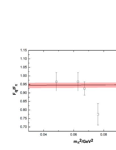
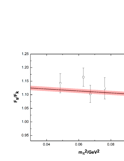
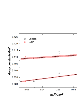
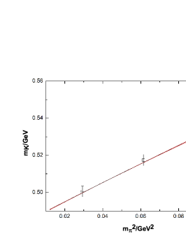
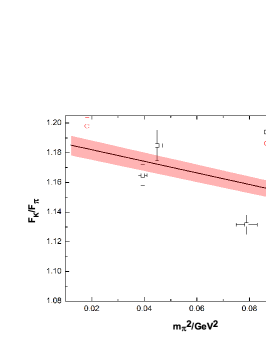
Remarkable progress has been made in recent years for the lattice calculation of the η\eta-η\eta^{\prime} system. Both their masses and mixing angles at different pion masses are obtained by many lattice collaborations. In this work, we fix the unknown low-energy constants (LECs) of by performing fits to relevant lattice data, including the η\eta/η\eta^{\prime} masses and their mixing angle at different mπm_{\pi}, the weak decay constants of pion and kaon, and the pion-mass dependences of mKm_{K}. Apart from the lattice data of the η\eta/η\eta^{\prime} masses at unphysically large mπm_{\pi} from the ETMC [46], UKQCD [47], RBC/UKQCD [48], HSC [49] that have been analyzed in Refs. [42, 44], we also include the new results from the RQCD collaboration [50] in the present study. In order to make direct comparisons of other data, only the lattice simulations with physical strange quark mass from Ref. [50] are taken into account here. The various lattice data of the masses for η\eta and η\eta^{\prime} are shown in the left panel of Fig. 1, together with their mixing angles in the quark-flavor base in the right panel. To be in accordance with the lattice setup, we take the average of θq\theta_{q} and θs\theta_{s} to fit the latter data set. It is noted that the phenomenological determinations also favor rather similar values for θq\theta_{q} and θs\theta_{s} [51, 52, 42]. The decay constants FqF_{q} and FsF_{s} defined in the mixing matrix of the quark-flavor base as functions of pion masses are provided by the lattice study [46] and we will take these kinds of data in our fits too, as shown in Fig. 2. For the pion-mass dependences of the Fπ,FKF_{\pi},F_{K} and mKm_{K}, we take into account the lattice data up to mπ2=0.1m_{\pi}^{2}=0.1 GeV2, as explicitly illustrated in Fig. 3.

Parameters NLO Fit
F(MeV)F({\rm MeV}) 91.050.44+0.4291.05^{+0.42}_{-0.44}
103×L510^{3}\times L_{5} 1.680.06+0.051.68^{+0.05}_{-0.06}
103×L810^{3}\times L_{8} 0.880.04+0.040.88^{+0.04}_{-0.04}
Λ1\Lambda_{1} 0.170.05+0.05-0.17^{+0.05}_{-0.05}
Λ2\Lambda_{2} 0.060.09+0.080.06^{+0.08}_{-0.09}
χ2/(d.o.f)\chi^{2}/(d.o.f) 219.9/(1115)219.9/(111-5)
Table 1: The values of the LECs from the NLO fit.
Refer to caption
Refer to caption
Figure 1: The masses of η\eta and η\eta^{\prime} as functions of mπm_{\pi} (left panel) and the pion-mass dependences of the η\eta-η\eta^{\prime} mixing angle in the quark-flavor basis (right panel). The lattice data of the η/η\eta/\eta^{\prime} masses are taken from ETMC [46], UKQCD [47], RBC/UKQCD [48], HSC [49] and RQCD [50]. For the η/η\eta/\eta^{\prime} masses from Ref. [50], only the results from the ensemble with approximately physical mass of strange quark are included. The lattice data of mixing angles in the quark-flavor base are taken from Ref. [46].
Refer to caption
Refer to caption
Figure 2: The decay constants of FqF_{q} and FsF_{s} defined in Eq. (128) as functions of mπm_{\pi}. The lattice data are taken from Ref. [46].
Refer to caption
Refer to caption
Refer to caption
Figure 3: The pion-mass dependences of FπF_{\pi}, FKF_{K} and mKm_{K}. The lattice data in the left and central panels are from Refs. [53, 54]. The data in the right panel are from Ref. [55].

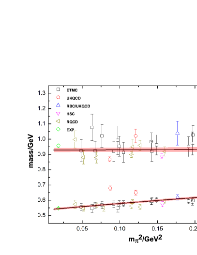
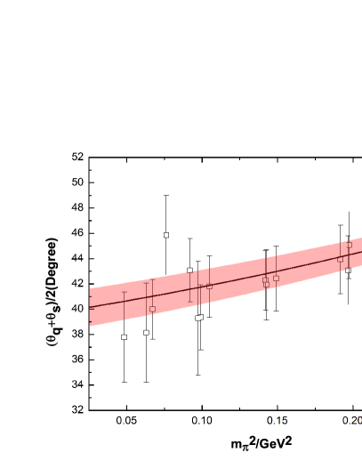
The values of the LECs from the fits are summarized in Table 1. The resulting curves for the masses of η\eta and η\eta^{\prime} and their mixing angles from the fits are given in Fig. 1. It is noted that the LO fit to the masses of η\eta and η\eta^{\prime} with just the single parameter M0M_{0} can reasonably reproduce the lattice data with M0=820M_{0}=820 MeV [42, 44]. Therefore we will fix M0M_{0} at this value during the NLO fits. It is verified that by releasing the M0M_{0} the fits do not improve and the values of the parameters in Table 1 barely change. The resulting parameters from the revised NLO fits are close to the previous ones given in Refs. [42, 44]. With the fitted parameters in Table 1, we are ready to predict the important quantities related with the axion.

Since the bare mass of the axion, i.e. ma,0m_{a,0} in Eq. (1), is explicitly kept throughout our calculations, e.g. Eqs. (59), (23)-(27) and (4), it is straightforward for us to explore the so-called axion-like scenarios by assigning some specific nonvanishing values to ma,0m_{a,0}. Nevertheless, in this work we will mainly focus on the phenomenological predictions for the QCD-axion scenario by taking ma,0=0m_{a,0}=0 in Eq. (1). The explicit values of the transition matrix elements in Eq. (100) between the physical states of π^0,η^,η^,a^\hat{\pi}^{0},\hat{\eta},\hat{\eta}^{\prime},\hat{a} and the bare states of π0,η8,η0,a\pi^{0},\eta_{8},\eta_{0},a are determined to be

(π^0η^η^a^)=MLO+NLO(π0η8η0a),\displaystyle\left(\begin{array}[]{c}\hat{\pi}^{0}\\ \hat{\eta}\\ \hat{\eta}^{\prime}\\ \hat{a}\end{array}\right)=M^{\rm LO+NLO}\left(\begin{array}[]{c}\pi^{0}\\ \eta_{8}\\ \eta_{0}\\ a\end{array}\right)\,, (137)

with

MLO+NLO=\displaystyle M^{\rm LO+NLO}=
(1+(0.015±0.001)0.017+(0.010±0.001)0.009+(0.007±0.001)12.1+(0.48±0.08)fa0.019+(0.007±0.001)0.94+(0.21±0.01)0.33+(0.22±0.03)34.3+(0.9±0.2)fa0.003+(0.003±0.000)0.33+(0.18±0.03)0.94+(0.13±0.02)25.9+(0.5±0.1)fa12.1+(0.20±0.03)fa23.8+(1.60.8+0.8)fa35.7+(5.71.7+1.6)fa1+27.6±1.0fa2),\displaystyle{\tiny\left(\begin{array}[]{cccc}1+(0.015\pm 0.001)&0.017+(-0.010\pm 0.001)&0.009+(-0.007\pm 0.001)&\frac{12.1+(0.48\pm 0.08)}{f_{a}}\\ -0.019+(0.007\pm 0.001)&0.94+(0.21\pm 0.01)&0.33+(-0.22\pm 0.03)&\frac{34.3+(0.9\pm 0.2)}{f_{a}}\\ -0.003+(-0.003\pm 0.000)&-0.33+(-0.18\pm 0.03)&0.94+(0.13\pm 0.02)&\frac{25.9+(-0.5\pm 0.1)}{f_{a}}\\ \frac{-12.1+(-0.20\pm 0.03)}{f_{a}}&\frac{-23.8+(1.6^{+0.8}_{-0.8})}{f_{a}}&\frac{-35.7+(-5.7^{+1.6}_{-1.7})}{f_{a}}&1+\frac{27.6\pm 1.0}{f_{a}^{2}}\end{array}\right)\,,} (142)

where the first and second entries in each matrix element correspond to the LO and NLO contributions, respectively. For the numbers in the last row and last column accompanying 1/fa1/f_{a}, they are given in units of MeV, while the number accompanying 1/fa21/f_{a}^{2} is given in units of MeV2. The main focus of our work is the relative corrections from the NLO part compared to the LO one.

For the mixing strengths between the π^0\hat{\pi}^{0} and η0,8\eta_{0,8}, and also the mixing between the η^()\hat{\eta}^{(^{\prime})} and the π0\pi^{0}, which are all proportional to the leading IB factor ϵ\epsilon, the NLO parts in the δ\delta counting gives rather large relative corrections compared to the LO results, ranging from around 60% up to 100%. For the η\eta-η\eta^{\prime} mixing, it is also found that the NLO contribution can be as large as around 60% relative to the LO part. However, it is interesting to note that all the mixing strengths between the axion and the light-flavor pseudoscalar π0,η,η\pi^{0},\eta,\eta^{\prime}, i.e. the numbers in the last column and the last row, the relative NLO corrections in the δ\delta counting to the LO parts are small, ranging from around 2% up to around 15%. The uncertainties of the mixing strengths given in Eq. (4), estimated by the using the error bands of the LECs in Table 1, turn out to be mild as well.

The contributions from the LO and NLO parts to the mass squared of the light-flavor pseudoscalar mesons and the axion in Eqs. (56)-(60) are found to be

mπ^\displaystyle m_{\hat{\pi}} =\displaystyle= [134.90+(0.10±0.07)]MeV,\displaystyle\big{[}134.90+(0.10\pm 0.07)\big{]}{\rm MeV}\,,
mK^\displaystyle m_{\hat{K}} =\displaystyle= [489.2+(5.03.5+3.4)]MeV,\displaystyle\big{[}489.2+(5.0^{+3.4}_{-3.5})\big{]}{\rm MeV}\,,
mη^\displaystyle m_{\hat{\eta}} =\displaystyle= [490.2+(60.910.0+10.2)]MeV,\displaystyle\big{[}490.2+(60.9^{+10.2}_{-10.0})\big{]}{\rm MeV}\,,
mη^\displaystyle m_{\hat{\eta}^{\prime}} =\displaystyle= [954.3+(28.412.6+11.9)]MeV,\displaystyle\big{[}954.3+(-28.4^{+11.9}_{-12.6})\big{]}{\rm MeV}\,,
ma^\displaystyle m_{\hat{a}} =\displaystyle= [5.96+(0.12±0.02)]μeV1012GeVfa,\displaystyle\big{[}5.96+(0.12\pm 0.02)\big{]}\mu{\rm eV}\frac{10^{12}{\rm GeV}}{f_{a}}\,, (144)

where the first and second entries inside the square brackets denote the results from the LO and NLO terms, respectively. Comparing with the LO case, it is clear that the NLO correction brings the η\eta mass much closer to its physical value. When compared with the LO case, the NLO correction brings the η\eta mass much closer to its physical value, although it somewhat worsens the description of the η\eta^{\prime} mass. However, we should notice that while the NLO contribution to the η\eta^{\prime} mass is quite small, less than 3% of the LO value, it is a 12% for the η\eta mass, which allows us to match its experimental value. The NLO contribution to the axion mass turns out to be rather small.

5 Two-photon couplings

Relying on the previous results of the mixing relations, we are ready to study the two-photon decays of the π0,η,η\pi^{0},\eta,\eta^{\prime} and aa, based on the LO and NLO WZW operators in Eqs. (8) and (2), respectively. By inserting the mixing relations (86) into the LO WZW Lagrangian (8) and neglecting all the IB terms, the two-photon couplings of the physical states read

WZWLO=\displaystyle\mathcal{L}_{WZW}^{\rm LO}= 32e28π2FεμνρσμAνρAσ{1+x1132π^0\displaystyle-\frac{3\sqrt{2}e^{2}}{8\pi^{2}F}\varepsilon_{\mu\nu\rho\sigma}\partial^{\mu}A^{\nu}\partial^{\rho}A^{\sigma}\bigg{\{}\frac{1+x_{11}}{3\sqrt{2}}\hat{\pi}^{0} (145)
+[cθ22sθ36(1+x22)+sθ+22cθ36(x23y23)]η^+\displaystyle+\bigg{[}\frac{c_{\theta}-2\sqrt{2}s_{\theta}}{3\sqrt{6}}(1+x_{22})+\frac{s_{\theta}+2\sqrt{2}c_{\theta}}{3\sqrt{6}}(x_{23}-y_{23})\bigg{]}\hat{\eta}+
+[sθ+22cθ36(1+x33)+cθ22sθ36(x23+y23)]η^+\displaystyle+\bigg{[}\frac{s_{\theta}+2\sqrt{2}c_{\theta}}{3\sqrt{6}}(1+x_{33})+\frac{c_{\theta}-2\sqrt{2}s_{\theta}}{3\sqrt{6}}(x_{23}+y_{23})\bigg{]}\hat{\eta}^{\prime}+
+[(cθ22sθ)v24+(sθ+22cθ)v3436\displaystyle+\bigg{[}\frac{(c_{\theta}-2\sqrt{2}s_{\theta})v_{24}+(s_{\theta}+2\sqrt{2}c_{\theta})v_{34}}{3\sqrt{6}}
+(cθ22sθ)(x24+y24)+(sθ+22cθ)(x34+y34)36]a^},\displaystyle\qquad+\frac{(c_{\theta}-2\sqrt{2}s_{\theta})(x_{24}+y_{24})+(s_{\theta}+2\sqrt{2}c_{\theta})(x_{34}+y_{34})}{3\sqrt{6}}\bigg{]}\hat{a}\bigg{\}}\,,

where all of the NLO terms are introduced through the mixing. Since we stick to the NLO calculation, only the LO mixing relations (22) are needed to insert into the NLO WZW Lagrangian (2) and the resulting two-photon interactions are given by

WZWNLO=\displaystyle\mathcal{L}_{WZW}^{\rm NLO}= e2FεμνρσμAνρAσ{32mπ2t13π^0\displaystyle\frac{e^{2}}{F}\varepsilon_{\mu\nu\rho\sigma}\partial^{\mu}A^{\nu}\partial^{\rho}A^{\sigma}\bigg{\{}\frac{32m_{\pi}^{2}t_{1}}{3}\hat{\pi}^{0}
+3293{92sθk3+t1[cθ(7mπ24mK2)22sθ(mK2+2mπ2)]}η^\displaystyle+\frac{32}{9\sqrt{3}}\big{\{}-9\sqrt{2}s_{\theta}k_{3}+t_{1}\big{[}c_{\theta}(7m_{\pi}^{2}-4m_{K}^{2})-2\sqrt{2}s_{\theta}(m_{K}^{2}+2m_{\pi}^{2})\big{]}\big{\}}\hat{\eta}
+3293{92cθk3+t1[22cθ(2mπ2+mK2)+sθ(7mπ24mK2)]}η^\displaystyle+\frac{32}{9\sqrt{3}}\big{\{}9\sqrt{2}c_{\theta}k_{3}+t_{1}\big{[}2\sqrt{2}c_{\theta}(2m_{\pi}^{2}+m_{K}^{2})+s_{\theta}(7m_{\pi}^{2}-4m_{K}^{2})\big{]}\big{\}}\hat{\eta}^{\prime}
+3227{9k3(Ffa6sθv24+6cθv34)\displaystyle+\frac{32}{27}\big{\{}9k_{3}\big{(}\frac{F}{f_{a}}-\sqrt{6}s_{\theta}v_{24}+\sqrt{6}c_{\theta}v_{34}\big{)}
+t1[3sθ(42v24mπ27v34mπ2+22v24mK2+4v34mK2)\displaystyle\qquad\quad\,\,+t_{1}\big{[}-\sqrt{3}s_{\theta}(4\sqrt{2}v_{24}m_{\pi}^{2}-7v_{34}m_{\pi}^{2}+2\sqrt{2}v_{24}m_{K}^{2}+4v_{34}m_{K}^{2})
+3cθ(42v34mπ2+7v24mπ2+22v34mK24v34mK2)]}a^}.\displaystyle\qquad\qquad\qquad+\sqrt{3}c_{\theta}(4\sqrt{2}v_{34}m_{\pi}^{2}+7v_{24}m_{\pi}^{2}+2\sqrt{2}v_{34}m_{K}^{2}-4v_{34}m_{K}^{2})\big{]}\big{\}}\hat{a}\bigg{\}}\,.

The two-photon decay amplitude of ϕγ(k1)γ(k2)\phi\to\gamma(k_{1})\gamma(k_{2}) with ϕ=π0,η,η\phi=\pi^{0},\eta,\eta^{\prime} and aa can be written as

Tϕγγ=e2εμνρσk1μϵ1νk2ρϵ2σFϕγγ,\displaystyle T_{\phi\to\gamma\gamma}=e^{2}\varepsilon_{\mu\nu\rho\sigma}k_{1}^{\mu}\epsilon_{1}^{\nu}k_{2}^{\rho}\epsilon_{2}^{\sigma}F_{\phi\gamma\gamma}\,, (147)

where the two-photon coupling strengths FϕγγF_{\phi\gamma\gamma} read

Fπ0γγ=14π2F+14π2Fx11643Ft1mπ2,\displaystyle F_{\pi^{0}\gamma\gamma}=\frac{1}{4\pi^{2}F}+\frac{1}{4\pi^{2}F}x_{11}-\frac{64}{3F}t_{1}m_{\pi}^{2}\,, (148)
Fηγγ=\displaystyle F_{\eta\gamma\gamma}= cθ22sθ43π2F(1+x22)+sθ+22cθ43π2F(x23y23)+6463Fsθk3\displaystyle\frac{c_{\theta}-2\sqrt{2}s_{\theta}}{4\sqrt{3}\pi^{2}F}(1+x_{22})+\frac{s_{\theta}+2\sqrt{2}c_{\theta}}{4\sqrt{3}\pi^{2}F}(x_{23}-y_{23})+\frac{64\sqrt{6}}{3F}s_{\theta}k_{3} (149)
64327Ft1[cθ(7mπ24mK2)22sθ(mK2+2mπ2)],\displaystyle-\frac{64\sqrt{3}}{27F}t_{1}\bigg{[}c_{\theta}(7m_{\pi}^{2}-4m_{K}^{2})-2\sqrt{2}s_{\theta}(m_{K}^{2}+2m_{\pi}^{2})\bigg{]}\,,
Fηγγ=\displaystyle F_{\eta^{\prime}\gamma\gamma}= sθ+22cθ43π2F(1+x33)+cθ22sθ43π2F(x23+y23)6463Fcθk3\displaystyle\frac{s_{\theta}+2\sqrt{2}c_{\theta}}{4\sqrt{3}\pi^{2}F}(1+x_{33})+\frac{c_{\theta}-2\sqrt{2}s_{\theta}}{4\sqrt{3}\pi^{2}F}(x_{23}+y_{23})-\frac{64\sqrt{6}}{3F}c_{\theta}k_{3} (150)
64327Ft1[sθ(7mπ24mK2)+22cθ(mK2+2mπ2)],\displaystyle-\frac{64\sqrt{3}}{27F}t_{1}\bigg{[}s_{\theta}(7m_{\pi}^{2}-4m_{K}^{2})+2\sqrt{2}c_{\theta}(m_{K}^{2}+2m_{\pi}^{2})\bigg{]}\,,
Faγγ=(cθ22sθ)v24+(sθ+22cθ)v3443π2F\displaystyle F_{a\gamma\gamma}=\frac{(c_{\theta}-2\sqrt{2}s_{\theta})v_{24}+(s_{\theta}+2\sqrt{2}c_{\theta})v_{34}}{4\sqrt{3}\pi^{2}F}
+(cθ22sθ)(x24+y24)+(sθ+22cθ)(x34+y34)43π2F6463Fk3(Ffa6sθv24+6cθv34)\displaystyle+\frac{(c_{\theta}-2\sqrt{2}s_{\theta})(x_{24}+y_{24})+(s_{\theta}+2\sqrt{2}c_{\theta})(x_{34}+y_{34})}{4\sqrt{3}\pi^{2}F}-\frac{64\sqrt{6}}{3F}k_{3}\bigg{(}\frac{F}{f_{a}}-\sqrt{6}s_{\theta}v_{24}+\sqrt{6}c_{\theta}v_{34}\bigg{)}
6427Ft1[3sθ(42v24mπ27v34mπ2+22v24mK2+4v34mK2)\displaystyle-\frac{64}{27F}t_{1}\bigg{[}-\sqrt{3}s_{\theta}(4\sqrt{2}v_{24}m_{\pi}^{2}-7v_{34}m_{\pi}^{2}+2\sqrt{2}v_{24}m_{K}^{2}+4v_{34}m_{K}^{2})
+3cθ(42v34mπ2+7v24mπ2+22v34mK24v24mK2)].\displaystyle\qquad\qquad+\sqrt{3}c_{\theta}(4\sqrt{2}v_{34}m_{\pi}^{2}+7v_{24}m_{\pi}^{2}+2\sqrt{2}v_{34}m_{K}^{2}-4v_{24}m_{K}^{2})\bigg{]}\,. (151)

We use the decay widths of π0γγ\pi^{0}\to\gamma\gamma, ηγγ\eta\to\gamma\gamma and ηγγ\eta^{\prime}\to\gamma\gamma from the most recent PDG average [56] to estimate their two-photon couplings

Fπ0γγExp\displaystyle F_{\pi^{0}\gamma\gamma}^{\rm Exp} =\displaystyle= 0.274±0.002 GeV1,\displaystyle 0.274\pm 0.002\text{ GeV}^{-1}\,, (152)
FηγγExp\displaystyle F_{\eta\gamma\gamma}^{\rm Exp} =\displaystyle= 0.274±0.006 GeV1,\displaystyle 0.274\pm 0.006\text{ GeV}^{-1}\,, (153)
FηγγExp\displaystyle F_{\eta^{\prime}\gamma\gamma}^{\rm Exp} =\displaystyle= 0.344±0.008 GeV1.\displaystyle 0.344\pm 0.008\text{ GeV}^{-1}\,. (154)

Those couplings can be then exploited to determine the NLO LECs from the WZW Lagrangian (9) entering in Eqs. (148)-(150). Their explicit values turn out to be

t1=(4.4±2.3)×104GeV2,k3=(1.25±0.23)×104,\displaystyle t_{1}=-(4.4\pm 2.3)\times 10^{-4}{\rm GeV}^{-2}\,,\qquad k_{3}=(1.25\pm 0.23)\times 10^{-4}\,, (155)

leading to

Fπ0γγ\displaystyle F_{\pi^{0}\gamma\gamma} =\displaystyle= 0.276±0.001 GeV1,\displaystyle 0.276\pm 0.001\text{ GeV}^{-1}\,, (156)
Fηγγ\displaystyle F_{\eta\gamma\gamma} =\displaystyle= 0.276±0.009 GeV1,\displaystyle 0.276\pm 0.009\text{ GeV}^{-1}\,, (157)
Fηγγ\displaystyle F_{\eta^{\prime}\gamma\gamma} =\displaystyle= 0.343±0.012 GeV1,\displaystyle 0.343\pm 0.012\text{ GeV}^{-1}\,, (158)

which perfectly reproduce the experimental inputs.

With the values of the NLO LECs of WZWNLO{\cal L}_{WZW}^{\rm NLO} in Eq. (155) and the fitted parameters in Table 1, we can now give our prediction to the two-photon coupling of the axion FaγγF_{a\gamma\gamma} up to NLO in the δ\delta counting

Faγγ=[20.1+(0.5±0.1)]×103fa,\displaystyle F_{a\gamma\gamma}=-\frac{[20.1+(0.5\pm 0.1)]\times 10^{-3}}{f_{a}}\,, (159)

where the first entry in the numerator on the right hand side corresponds to the LO contribution and the second one denotes the NLO contribution. The two-photon coupling FaγγF_{a\gamma\gamma} is related with the gaγγg_{a\gamma\gamma} used in Refs. [29, 45] via

gaγγ=4παemFaγγ=αem2πfa(1.63±0.01),\displaystyle g_{a\gamma\gamma}=4\pi\alpha_{em}F_{a\gamma\gamma}=-\frac{\alpha_{em}}{2\pi f_{a}}\big{(}1.63\pm 0.01\big{)}\,, (160)

where the numbers inside the bracket can be compared to the results of 1.92±0.041.92\pm 0.04 [29] and 2.05±0.032.05\pm 0.03 [45] from the SU(2)SU(2) and SU(3)SU(3) χ\chiPT analyses up to NLO, respectively. The determination of the magnitude of gaγγg_{a\gamma\gamma} from the NLO U(3)U(3) calculation looks a bit smaller than those from the NLO studies in the SU(2)SU(2) and SU(3)SU(3) cases. It is noted that the chiral loops start to appear at NLO in the SU(2)SU(2) and SU(3)SU(3) χ\chiPT in the conventional chiral power counting. While, in the δ\delta-counting scheme, the chiral loops only enter at NNLO in the U(3)U(3) χ\chiPT. To consistently take into account all the pieces of the two-photon coupling of the axion at NNLO in the U(3)U(3) χ\chiPT, one also needs to extend the axion-meson mixing calculations at the same order and we leave this task to a future work.

6 Summary and Conclusions

In this work, U(3)U(3) chiral perturbation theory is demonstrated to be able to provide a useful framework to calculate the matrix elements of the mixing between the π0,η,η\pi^{0},\eta,\eta^{\prime} and the axion order by order in the joint expansions of the momenta, light-quark masses and 1/NC1/N_{C}, i.e. the δ\delta-counting scheme. We have performed the complete calculation of the axion-meson mixing and the two-photon couplings of the axion and light-flavor pseudoscalar mesons up to NLO in the δ\delta-counting rule within the framework of the U(3)U(3) chiral perturbation theory. The unknown chiral low-energy constants are fixed through the fits to a large amount of lattice QCD data, consisting of the pion-mass dependences of η\eta-η\eta^{\prime} mixing data, kaon mass, and the decay constants of the pion and kaon. Reasonable reproductions of the various lattice data are achieved with the U(3)U(3) contributions up to NLO. The mixing matrix elements of the π0,η,η\pi^{0},\eta,\eta^{\prime} and the axion are then further used to calculate their two-photon couplings, together with the NLO Wess-Zumino-Witten Lagrangian, where the parameters in the latter Lagrangian are fixed by the experimental two-photon couplings of the π0,η\pi^{0},\eta and η\eta^{\prime}.

The determined chiral low-energy constants are then used to predict the QCD-axion masses, the mixing strengths of the axion and the π0,η,η\pi^{0},\eta,\eta^{\prime}, and the two-photon coupling of the QCD axion. The NLO contributions in the δ\delta counting to the various axion quantities relative to the LO ones are found to be small. This work paves the way to systematically calculate the interactions between the axion and the light-flavor pseudoscalar mesons π,K,η\pi,K,\eta and η\eta^{\prime} order by order in the joint expansions of momenta, light-quark masses and 1/NC1/N_{C}.

Acknowledgements

We would like to thank Luca Di Luzio for interesting discussions, and Gunnar Bali and Jakob Simeth for communications to clarify the lattice data of RQCD. This work is funded in part by the Natural Science Foundation of China (NSFC) under Grants Nos. 12150013, 11975090, 12047503, and by the Science Foundation of Hebei Normal University with contract No. L2023B09. ZHG appreciates the support of Peng Huan-Wu visiting professorship and the hospitality of Institute of Theoretical Physics at Chinese Academy of Sciences, where part of this work has been done. JAO would like to thank partial support by the MICINN AEI (Spain) Grant No. PID2019–106080GB-C22/AEI/10.13039/501100011033, and by the EU Horizon 2020 research and innovation programme, STRONG-2020 project, under Grant agreement No. 824093. RG is partially funded by the Hebei Province Graduate Innovation Funding Project with contract number CXZZBS2023085.

Appendix: Next-to-leading order coefficients for bilinear terms

Substituting the LO mixing relations of Eq. (22) into the NLO Lagrangian (7), one can calculate all the NLO pieces of the bilinear terms in Eq. (35) and their explicit expressions read

δkπη=\displaystyle\delta^{\pi\eta}_{k}= 8L53F2{2v12[mK2(2cθ2+22cθsθ+sθ2)mπ2(2+22cθsθsθ2)]+3ϵ(2sθcθ)\displaystyle\dfrac{-8L_{5}}{3F^{2}}\bigg{\{}2v_{12}\big{[}m^{2}_{K}(2c^{2}_{\theta}+2\sqrt{2}c_{\theta}s_{\theta}+s^{2}_{\theta})-m^{2}_{\pi}(2+2\sqrt{2}c_{\theta}s_{\theta}-s^{2}_{\theta})\big{]}+\sqrt{3}\epsilon(\sqrt{2}s_{\theta}-c_{\theta}) (161)
2v13(mK2mπ2)(2cθ2cθsθ2sθ2)}+Λ1sθ(cθv13sθv12),\displaystyle-2v_{13}(m^{2}_{K}-m^{2}_{\pi})(\sqrt{2}c^{2}_{\theta}-c_{\theta}s_{\theta}-\sqrt{2}s^{2}_{\theta})\bigg{\}}+\Lambda_{1}s_{\theta}(c_{\theta}v_{13}-s_{\theta}v_{12}),
δm2πη=\displaystyle\delta^{\pi\eta}_{m^{2}}= 16L83F2[4v12mK2(mK2mπ2)(2cθ2+22cθsθ+sθ2)4v13mK2(mK2mπ2)(2cθ2cθsθ\displaystyle-\dfrac{16L_{8}}{3F^{2}}\big{[}4v_{12}m^{2}_{K}(m^{2}_{K}-m^{2}_{\pi})(2c^{2}_{\theta}+2\sqrt{2}c_{\theta}s_{\theta}+s^{2}_{\theta})-4v_{13}m^{2}_{K}(m^{2}_{K}-m^{2}_{\pi})(\sqrt{2}c^{2}_{\theta}-c_{\theta}s_{\theta} (162)
2sθ2)23mπ2ϵ(cθ2sθ)]Λ23{2v12sθ[2mK2(2cθ+sθ)+mπ2(sθ22cθ)]\displaystyle-\sqrt{2}s^{2}_{\theta})-2\sqrt{3}m^{2}_{\pi}\epsilon(c_{\theta}-\sqrt{2}s_{\theta})\big{]}-\dfrac{\Lambda_{2}}{3}\bigg{\{}2v_{12}s_{\theta}\big{[}2m^{2}_{K}(\sqrt{2}c_{\theta}+s_{\theta})+m^{2}_{\pi}(s_{\theta}-2\sqrt{2}c_{\theta})\big{]}
+2v13[mK2(2cθ22cθsθ+2sθ2)+mπ2(2cθ2cθsθ2sθ2)]+6sθϵ},\displaystyle+2v_{13}\big{[}m^{2}_{K}(-\sqrt{2}c^{2}_{\theta}-2c_{\theta}s_{\theta}+\sqrt{2}s^{2}_{\theta})+m^{2}_{\pi}(\sqrt{2}c^{2}_{\theta}-c_{\theta}s_{\theta}-\sqrt{2}s^{2}_{\theta})\big{]}+\sqrt{6}s_{\theta}\epsilon\bigg{\}}\,,
δkπη=\displaystyle\delta^{\pi{\eta}^{\prime}}_{k}= 8L53F2{2v12(mK2mπ2)(2cθ2cθsθ2sθ2)+3ϵ(2cθ+sθ)+2v13[mK2(cθ2\displaystyle\dfrac{8L_{5}}{3F^{2}}\bigg{\{}2v_{12}(m^{2}_{K}-m^{2}_{\pi})(\sqrt{2}c^{2}_{\theta}-c_{\theta}s_{\theta}-\sqrt{2}s^{2}_{\theta})+\sqrt{3}\epsilon(\sqrt{2}c_{\theta}+s_{\theta})+2v_{13}\big{[}-m^{2}_{K}(c^{2}_{\theta} (163)
22cθsθ+2sθ2)+mπ2(222cθsθcθ2)]}+Λ1cθ(cθv13+sθv12),\displaystyle-2\sqrt{2}c_{\theta}s_{\theta}+2s^{2}_{\theta})+m^{2}_{\pi}(2-2\sqrt{2}c_{\theta}s_{\theta}-c^{2}_{\theta})\big{]}\bigg{\}}+\Lambda_{1}c_{\theta}(-c_{\theta}v_{13}+s_{\theta}v_{12})\,,
δm2πη=\displaystyle\delta^{\pi{\eta}^{\prime}}_{m^{2}}= 16L83F2[4v12mK2(mK2mπ2)(2cθ2cθsθ2sθ2)4v13mK2(mK2mπ2)(cθ222cθsθ+2sθ2)\displaystyle\dfrac{16L_{8}}{3F^{2}}\big{[}4v_{12}m^{2}_{K}(m^{2}_{K}-m^{2}_{\pi})(\sqrt{2}c^{2}_{\theta}-c_{\theta}s_{\theta}-\sqrt{2}s^{2}_{\theta})-4v_{13}m^{2}_{K}(m^{2}_{K}-m^{2}_{\pi})(c^{2}_{\theta}-2\sqrt{2}c_{\theta}s_{\theta}+2s^{2}_{\theta}) (164)
+23mπ2ϵ(2cθ+sθ)]+Λ23{2v13cθ[2mK2(cθ+2sθ)mπ2(cθ+22sθ)]\displaystyle+2\sqrt{3}m^{2}_{\pi}\epsilon(\sqrt{2}c_{\theta}+s_{\theta})\big{]}+\dfrac{\Lambda_{2}}{3}\bigg{\{}2v_{13}c_{\theta}\big{[}2m^{2}_{K}(-c_{\theta}+\sqrt{2}s_{\theta})-m^{2}_{\pi}(c_{\theta}+2\sqrt{2}s_{\theta})\big{]}
+2v12[mK2(2cθ2+2cθsθ2sθ2)+mπ2(2cθ2+cθsθ+2sθ2)]+6cθϵ},\displaystyle+2v_{12}\big{[}m^{2}_{K}(\sqrt{2}c^{2}_{\theta}+2c_{\theta}s_{\theta}-\sqrt{2}s^{2}_{\theta})+m^{2}_{\pi}(-\sqrt{2}c^{2}_{\theta}+c_{\theta}s_{\theta}+\sqrt{2}s^{2}_{\theta})\big{]}+\sqrt{6}c_{\theta}\epsilon\bigg{\}}\,,
δka=\displaystyle\delta^{a}_{k}= 8L53F2{v242[2mK2(2cθ2+22cθsθ+sθ2)+mπ2(cθ242cθsθ+sθ2)]+4v24v34[mK2(2cθ2\displaystyle\dfrac{8L_{5}}{3F^{2}}\bigg{\{}v^{2}_{24}\big{[}2m^{2}_{K}(2c^{2}_{\theta}+2\sqrt{2}c_{\theta}s_{\theta}+s^{2}_{\theta})+m^{2}_{\pi}(-c^{2}_{\theta}-4\sqrt{2}c_{\theta}s_{\theta}+s^{2}_{\theta})\big{]}+4v_{24}v_{34}\big{[}m^{2}_{K}(-\sqrt{2}c^{2}_{\theta} (165)
+cθsθ+2sθ2)+mπ2(2cθ2cθsθ2sθ2)]+v234[2mK2(cθ222cθsθ+2sθ2)\displaystyle+c_{\theta}s_{\theta}+\sqrt{2}s^{2}_{\theta})+m^{2}_{\pi}(\sqrt{2}c^{2}_{\theta}-c_{\theta}s_{\theta}-\sqrt{2}s^{2}_{\theta})\big{]}+v^{2}_{34}\big{[}2m^{2}_{K}(c^{2}_{\theta}-2\sqrt{2}c_{\theta}s_{\theta}+2s^{2}_{\theta})
+mπ2(cθ2+42cθsθsθ2)]}+16Λ1{(Ffa)2+26(v34cθv24sθ)Ffa+6cθ2v342+6sθ2v242\displaystyle+m^{2}_{\pi}(c^{2}_{\theta}+4\sqrt{2}c_{\theta}s_{\theta}-s^{2}_{\theta})\big{]}\bigg{\}}+\dfrac{1}{6}\Lambda_{1}\bigg{\{}\bigg{(}\frac{F}{f_{a}}\bigg{)}^{2}+2\sqrt{6}(v_{34}c_{\theta}-v_{24}s_{\theta})\frac{F}{f_{a}}+6c^{2}_{\theta}v^{2}_{34}+6s^{2}_{\theta}v^{2}_{24}
12cθsθv24v34},\displaystyle-12c_{\theta}s_{\theta}v_{24}v_{34}\bigg{\}}\,,
δkaπ=\displaystyle\delta^{a\pi}_{k}= 8L53F2{4cθ2mK2v12v24+mπ2[3v14+sθ2(v12v24+22v13v24+22v12v34+v13v34)\displaystyle\dfrac{8L_{5}}{3F^{2}}\bigg{\{}-4c_{\theta}^{2}m_{K}^{2}v_{12}v_{24}+m_{\pi}^{2}\big{[}3v_{14}+s_{\theta}^{2}(-v_{12}v_{24}+2\sqrt{2}v_{13}v_{24}+2\sqrt{2}v_{12}v_{34}+v_{13}v_{34}) (166)
+2cθsθ(22v12v24+v13v24+v12v3422v13v34)+cθ2(v12v2422v13v24\displaystyle+2c_{\theta}s_{\theta}(2\sqrt{2}v_{12}v_{24}+v_{13}v_{24}+v_{12}v_{34}-2\sqrt{2}v_{13}v_{34})+c_{\theta}^{2}(v_{12}v_{24}-2\sqrt{2}v_{13}v_{24}
22v12v34v13v34)]+2mK2[cθ2(2v13v24+2v12v34v13v34)sθ2(v12v24\displaystyle-2\sqrt{2}v_{12}v_{34}-v_{13}v_{34})\big{]}+2m_{K}^{2}\big{[}c_{\theta}^{2}(\sqrt{2}v_{13}v_{24}+\sqrt{2}v_{12}v_{34}-v_{13}v_{34})-s_{\theta}^{2}(v_{12}v_{24}
+2v13v24+2v12v34+2v13v34)cθsθ(v1222v24+v12v34+v13v24v1322v34)]\displaystyle+\sqrt{2}v_{13}v_{24}+\sqrt{2}v_{12}v_{34}+2v_{13}v_{34})-c_{\theta}s_{\theta}(v_{12}2\sqrt{2}v_{24}+v_{12}v_{34}+v_{13}v_{24}-v_{13}2\sqrt{2}v_{34})\big{]}
+3[sθ(2v24+v34)+cθ(v24+2v34)]ϵ}+Λ1(v12sθv13cθ)(16Ffav24sθ+v34cθ),\displaystyle+\sqrt{3}\big{[}s_{\theta}(-\sqrt{2}v_{24}+v_{34})+c_{\theta}(v_{24}+\sqrt{2}v_{34})\big{]}\epsilon\bigg{\}}+\Lambda_{1}(v_{12}s_{\theta}-v_{13}c_{\theta})\bigg{(}\dfrac{1}{\sqrt{6}}\dfrac{F}{f_{a}}-v_{24}s_{\theta}+v_{34}c_{\theta}\bigg{)}\,,
δkaη=\displaystyle\delta^{a\eta}_{k}= 8L53F2[2v24mK2(2cθ2+22cθsθ+sθ2)+v24mπ2(cθ242cθsθ+sθ2)2v34(mK2mπ2)\displaystyle\dfrac{8L_{5}}{3F^{2}}\big{[}2v_{24}m^{2}_{K}(2c^{2}_{\theta}+2\sqrt{2}c_{\theta}s_{\theta}+s^{2}_{\theta})+v_{24}m^{2}_{\pi}(-c^{2}_{\theta}-4\sqrt{2}c_{\theta}s_{\theta}+s^{2}_{\theta})-2v_{34}(m^{2}_{K}-m^{2}_{\pi}) (167)
(2cθ2cθsθ2sθ2)]+Λ1sθ(16Ffa+v24sθv34cθ),\displaystyle(\sqrt{2}c^{2}_{\theta}-c_{\theta}s_{\theta}-\sqrt{2}s^{2}_{\theta})\big{]}+\Lambda_{1}s_{\theta}\bigg{(}-\dfrac{1}{\sqrt{6}}\frac{F}{f_{a}}+v_{24}s_{\theta}-v_{34}c_{\theta}\bigg{)}\,,
δkaη=\displaystyle\delta^{a{\eta}^{\prime}}_{k}= 8L53F2[2v24(mK2mπ2)(2cθ2cθsθ2sθ2)2v34mK2(cθ222cθsθ+2sθ2)\displaystyle\dfrac{-8L_{5}}{3F^{2}}\big{[}2v_{24}(m^{2}_{K}-m^{2}_{\pi})(\sqrt{2}c^{2}_{\theta}-c_{\theta}s_{\theta}-\sqrt{2}s^{2}_{\theta})-2v_{34}m^{2}_{K}(c^{2}_{\theta}-2\sqrt{2}c_{\theta}s_{\theta}+2s^{2}_{\theta}) (168)
+v34mπ2(cθ242cθsθ+sθ2)]+Λ1cθ(16Ffav24sθ+v34cθ),\displaystyle+v_{34}m^{2}_{\pi}(-c^{2}_{\theta}-4\sqrt{2}c_{\theta}s_{\theta}+s^{2}_{\theta})\big{]}+\Lambda_{1}c_{\theta}\bigg{(}\dfrac{1}{\sqrt{6}}\frac{F}{f_{a}}-v_{24}s_{\theta}+v_{34}c_{\theta}\bigg{)}\,,
δma2=\displaystyle\delta_{m^{2}_{a}}= 16L83F2{8(2v242+v34v242v342)cθ(mK2mπ2)mK2sθ+cθ2[4(2v24222v34v24\displaystyle\frac{16L_{8}}{3F^{2}}\bigg{\{}8(\sqrt{2}v_{24}^{2}+v_{34}v_{24}-\sqrt{2}v_{34}^{2})c_{\theta}(m_{K}^{2}-m_{\pi}^{2})m_{K}^{2}s_{\theta}+c_{\theta}^{2}\big{[}4(2v_{24}^{2}-2\sqrt{2}v_{34}v_{24} (169)
+v342)mK44mπ2(2v24222v34v24+v342)mK2+3mπ4(v242+v342)]+sθ2[4(v242\displaystyle+v_{34}^{2})m_{K}^{4}-4m_{\pi}^{2}(2v_{24}^{2}-2\sqrt{2}v_{34}v_{24}+v_{34}^{2})m_{K}^{2}+3m_{\pi}^{4}(v_{24}^{2}+v_{34}^{2})\big{]}+s_{\theta}^{2}\big{[}4(v_{24}^{2}
+22v34v24+2v342)mK44mπ2(v242+22v34v24+2v342)mK2+3mπ4(v242+v342)]}\displaystyle+2\sqrt{2}v_{34}v_{24}+2v_{34}^{2})m_{K}^{4}-4m_{\pi}^{2}(v_{24}^{2}+2\sqrt{2}v_{34}v_{24}+2v_{34}^{2})m_{K}^{2}+3m_{\pi}^{4}(v_{24}^{2}+v_{34}^{2})\big{]}\bigg{\}}
+Λ29{v24[26mK2(2cθ+sθ)+6mπ2(22cθsθ)]Ffa+v34[26mK2(cθ2sθ)\displaystyle+\dfrac{\Lambda_{2}}{9}\bigg{\{}v_{24}\big{[}-2\sqrt{6}m^{2}_{K}(\sqrt{2}c_{\theta}+s_{\theta})+\sqrt{6}m^{2}_{\pi}(2\sqrt{2}c_{\theta}-s_{\theta})\big{]}\frac{F}{f_{a}}+v_{34}\big{[}2\sqrt{6}m^{2}_{K}(c_{\theta}-\sqrt{2}s_{\theta})
+6mπ2(cθ+22sθ)]Ffa+6v224[2mK2sθ(2cθ+sθ)+mπ2sθ(22cθ+sθ)]\displaystyle+\sqrt{6}m^{2}_{\pi}(c_{\theta}+2\sqrt{2}s_{\theta})\big{]}\frac{F}{f_{a}}+6v^{2}_{24}\big{[}2m^{2}_{K}s_{\theta}(\sqrt{2}c_{\theta}+s_{\theta})+m^{2}_{\pi}s_{\theta}(-2\sqrt{2}c_{\theta}+s_{\theta})\big{]}
+6v342[2mK2cθ(cθ2sθ)+mπ2cθ(cθ+22sθ)]+12v24v34[mK2(2cθ2+2cθsθ\displaystyle+6v^{2}_{34}\big{[}2m^{2}_{K}c_{\theta}(c_{\theta}-\sqrt{2}s_{\theta})+m^{2}_{\pi}c_{\theta}(c_{\theta}+2\sqrt{2}s_{\theta})\big{]}+12v_{24}v_{34}\big{[}-m^{2}_{K}(\sqrt{2}c^{2}_{\theta}+2c_{\theta}s_{\theta}
2sθ2)+mπ2(2cθ2cθsθ2sθ2)]},\displaystyle-\sqrt{2}s^{2}_{\theta})+m^{2}_{\pi}(\sqrt{2}c^{2}_{\theta}-c_{\theta}s_{\theta}-\sqrt{2}s^{2}_{\theta})\big{]}\bigg{\}}\,,
δm2aη=\displaystyle\delta^{a\eta}_{m^{2}}= 16L83F2{v24[4mK2(mK2mπ2)(2cθ2+22cθsθ+sθ2)+3mπ4]+4v34mK2(mK2mπ2)(2cθ2\displaystyle\dfrac{-16L_{8}}{3F^{2}}\bigg{\{}-v_{24}\big{[}4m^{2}_{K}(m^{2}_{K}-m^{2}_{\pi})(2c^{2}_{\theta}+2\sqrt{2}c_{\theta}s_{\theta}+s^{2}_{\theta})+3m^{4}_{\pi}\big{]}+4v_{34}m^{2}_{K}(m^{2}_{K}-m^{2}_{\pi})(\sqrt{2}c^{2}_{\theta} (170)
cθsθ2sθ2)}Λ218{[26mK2(2cθ+sθ)+6mπ2(22cθ+sθ)]Ffa\displaystyle-c_{\theta}s_{\theta}-\sqrt{2}s^{2}_{\theta})\bigg{\}}-\dfrac{\Lambda_{2}}{18}\bigg{\{}\big{[}2\sqrt{6}m^{2}_{K}(\sqrt{2}c_{\theta}+s_{\theta})+\sqrt{6}m^{2}_{\pi}(-2\sqrt{2}c_{\theta}+s_{\theta})\big{]}\frac{F}{f_{a}}
+12v24sθ[2mK2(2cθ+sθ)+mπ2(22cθsθ)]+12v34[mK2(2cθ2+2cθsθ2sθ2)\displaystyle+12v_{24}s_{\theta}\big{[}-2m^{2}_{K}(\sqrt{2}c_{\theta}+s_{\theta})+m^{2}_{\pi}(2\sqrt{2}c_{\theta}-s_{\theta})\big{]}+12v_{34}\big{[}m^{2}_{K}(\sqrt{2}c^{2}_{\theta}+2c_{\theta}s_{\theta}-\sqrt{2}s^{2}_{\theta})
+mπ2(2cθ2+cθsθ+2sθ2)]},\displaystyle+m^{2}_{\pi}(-\sqrt{2}c^{2}_{\theta}+c_{\theta}s_{\theta}+\sqrt{2}s^{2}_{\theta})\big{]}\bigg{\}}\,,
δm2aη=\displaystyle\delta^{a{\eta}^{\prime}}_{m^{2}}= 16L83F2{4v24mK2(mK2mπ2)(2cθ2cθsθ2sθ2)v34[4mK2(mK2mπ2)(cθ222cθsθ\displaystyle\dfrac{-16L_{8}}{3F^{2}}\bigg{\{}4v_{24}m^{2}_{K}(m^{2}_{K}-m^{2}_{\pi})(\sqrt{2}c^{2}_{\theta}-c_{\theta}s_{\theta}-\sqrt{2}s^{2}_{\theta})-v_{34}\big{[}4m^{2}_{K}(m^{2}_{K}-m^{2}_{\pi})(c^{2}_{\theta}-2\sqrt{2}c_{\theta}s_{\theta} (171)
+2sθ2)+3mπ4]}Λ218{[26mK2(cθ+2sθ)6mπ2(cθ+22sθ)]Ffa\displaystyle+2s^{2}_{\theta})+3m^{4}_{\pi}\big{]}\bigg{\}}-\dfrac{\Lambda_{2}}{18}\bigg{\{}\big{[}2\sqrt{6}m^{2}_{K}(-c_{\theta}+\sqrt{2}s_{\theta})-\sqrt{6}m^{2}_{\pi}(c_{\theta}+2\sqrt{2}s_{\theta})\big{]}\frac{F}{f_{a}}
+12v24[mK2(2cθ2+2cθsθ2sθ2)+mπ2(2cθ2+cθsθ+2sθ2)]\displaystyle+12v_{24}\big{[}m^{2}_{K}(\sqrt{2}c^{2}_{\theta}+2c_{\theta}s_{\theta}-\sqrt{2}s^{2}_{\theta})+m^{2}_{\pi}(-\sqrt{2}c^{2}_{\theta}+c_{\theta}s_{\theta}+\sqrt{2}s^{2}_{\theta})\big{]}
12v34cθ[2mK2(cθ2sθ)+mπ2(cθ+22sθ)]},\displaystyle-12v_{34}c_{\theta}\big{[}2m^{2}_{K}(c_{\theta}-\sqrt{2}s_{\theta})+m^{2}_{\pi}(c_{\theta}+2\sqrt{2}s_{\theta})\big{]}\bigg{\}}\,,
δm2aπ=\displaystyle\delta^{a\pi}_{m^{2}}= 16L83F2{4mK4[(2v12v242v13v242v12v34+v13v34)cθ2+sθ(v12(22v24+v34)\displaystyle\frac{16L_{8}}{3F^{2}}\bigg{\{}-4m_{K}^{4}\big{[}(2v_{12}v_{24}-\sqrt{2}v_{13}v_{24}-\sqrt{2}v_{12}v_{34}+v_{13}v_{34})c_{\theta}^{2}+s_{\theta}(v_{12}(2\sqrt{2}v_{24}+v_{34}) (172)
+v13(v2422v34))cθ+sθ2(v12v24+2v13v24+2v12v34+2v13v34)]\displaystyle+v_{13}(v_{24}-2\sqrt{2}v_{34}))c_{\theta}+s_{\theta}^{2}(v_{12}v_{24}+\sqrt{2}v_{13}v_{24}+\sqrt{2}v_{12}v_{34}+2v_{13}v_{34})\big{]}
+2mπ2[2cθ2(2v12v242v13v242v12v34+v13v34)mK2\displaystyle+2m_{\pi}^{2}\big{[}2c_{\theta}^{2}(2v_{12}v_{24}-\sqrt{2}v_{13}v_{24}-\sqrt{2}v_{12}v_{34}+v_{13}v_{34})m_{K}^{2}
+2cθsθ(22v12v24+v13v24+v12v3422v13v34)mK2+3ϵcθ(v24+2v34)\displaystyle+2c_{\theta}s_{\theta}(2\sqrt{2}v_{12}v_{24}+v_{13}v_{24}+v_{12}v_{34}-2\sqrt{2}v_{13}v_{34})m_{K}^{2}+\sqrt{3}\epsilon c_{\theta}(v_{24}+\sqrt{2}v_{34})
+sθ(2sθ(v12v24+2v13v24+2v12v34+2v13v34)mK2+3ϵ(v342v24))]\displaystyle+s_{\theta}(2s_{\theta}(v_{12}v_{24}+\sqrt{2}v_{13}v_{24}+\sqrt{2}v_{12}v_{34}+2v_{13}v_{34})m_{K}^{2}+\sqrt{3}\epsilon(v_{34}-\sqrt{2}v_{24}))\big{]}
+3mπ4[v14(cθ2+sθ2)(v12v24+v13v34)]}Λ218{6ϵ(Ffa6sθv24+6cθv34)\displaystyle+3m_{\pi}^{4}\big{[}v_{14}-(c_{\theta}^{2}+s_{\theta}^{2})(v_{12}v_{24}+v_{13}v_{34})\big{]}\bigg{\}}-\dfrac{\Lambda_{2}}{18}\bigg{\{}-6\epsilon\bigg{(}\frac{F}{f_{a}}-\sqrt{6}s_{\theta}v_{24}+\sqrt{6}c_{\theta}v_{34}\bigg{)}
+v12[26mK2(2cθ+sθ)+6mπ2(22cθsθ)]Ffa+v13[26mK2(cθ2sθ)\displaystyle+v_{12}\big{[}-2\sqrt{6}m^{2}_{K}(\sqrt{2}c_{\theta}+s_{\theta})+\sqrt{6}m^{2}_{\pi}(2\sqrt{2}c_{\theta}-s_{\theta})\big{]}\frac{F}{f_{a}}+v_{13}\big{[}2\sqrt{6}m^{2}_{K}(c_{\theta}-\sqrt{2}s_{\theta})
+6mπ2(cθ+22sθ)]Ffa+12v12v24sθ[2mK2(2cθ+sθ)+mπ2(22cθ+sθ)]\displaystyle+\sqrt{6}m^{2}_{\pi}(c_{\theta}+2\sqrt{2}s_{\theta})\big{]}\frac{F}{f_{a}}+12v_{12}v_{24}s_{\theta}\big{[}2m^{2}_{K}(\sqrt{2}c_{\theta}+s_{\theta})+m^{2}_{\pi}(-2\sqrt{2}c_{\theta}+s_{\theta})\big{]}
+12(v12v34+v13v24)[mK2(2cθ2+2cθsθ2sθ2)+mπ2(2cθ2cθsθ2sθ2)]\displaystyle+12(v_{12}v_{34}+v_{13}v_{24})\big{[}-m^{2}_{K}(\sqrt{2}c^{2}_{\theta}+2c_{\theta}s_{\theta}-\sqrt{2}s^{2}_{\theta})+m^{2}_{\pi}(\sqrt{2}c^{2}_{\theta}-c_{\theta}s_{\theta}-\sqrt{2}s^{2}_{\theta})\big{]}
+12v13v34cθ[2mK2(cθ2sθ)+mπ2(cθ+22sθ)]}.\displaystyle+12v_{13}v_{34}c_{\theta}\big{[}2m^{2}_{K}(c_{\theta}-\sqrt{2}s_{\theta})+m^{2}_{\pi}(c_{\theta}+2\sqrt{2}s_{\theta})\big{]}\bigg{\}}\,.
δkπ=8L5mπ2F2,\displaystyle\delta^{\pi}_{k}=\dfrac{8L_{5}m^{2}_{\pi}}{F^{2}}\,, (173)
δmπ2=16L8mπ4F2,\displaystyle\delta_{m^{2}_{\pi}}=\dfrac{16L_{8}m^{4}_{\pi}}{F^{2}}\,, (174)
δkK=8L5mK2F2,\displaystyle\delta^{K}_{k}=\dfrac{8L_{5}m^{2}_{K}}{F^{2}}\,, (175)
δmK2=16L8mK4F2,\displaystyle\delta_{m^{2}_{K}}=\dfrac{16L_{8}m^{4}_{K}}{F^{2}}\,, (176)
δkη=8L5[cθ2(4mK2mπ2)+42cθ(mK2mπ2)sθ+(2mK2+mπ2)sθ2]3F2+sθ2Λ1,\delta^{\eta}_{k}=\dfrac{8L_{5}[c_{\theta}^{2}(4m_{K}^{2}-m_{\pi}^{2})+4\sqrt{2}c_{\theta}(m_{K}^{2}-m_{\pi}^{2})s_{\theta}+(2m_{K}^{2}+m_{\pi}^{2})s_{\theta}^{2}]}{3F^{2}}+s_{\theta}^{2}\Lambda_{1}\,, (177)
δkη=8L5[cθ2(2mK2+mπ2)+42cθ(mK2+mπ2)sθ+(4mK2mπ2)sθ2]3F2+cθ2Λ1,\delta^{\eta^{\prime}}_{k}=\dfrac{8L_{5}[c_{\theta}^{2}(2m_{K}^{2}+m_{\pi}^{2})+4\sqrt{2}c_{\theta}(-m_{K}^{2}+m_{\pi}^{2})s_{\theta}+(4m_{K}^{2}-m_{\pi}^{2})s_{\theta}^{2}]}{3F^{2}}+c_{\theta}^{2}\Lambda_{1}\,, (178)
δkηη=16L5(mK2mπ2)(2cθ2cθsθ2sθ2)3F2cθsθΛ1,\delta^{\eta\eta^{\prime}}_{k}=-\dfrac{16L_{5}(m_{K}^{2}-m_{\pi}^{2})(\sqrt{2}c_{\theta}^{2}-c_{\theta}s_{\theta}-\sqrt{2}s_{\theta}^{2})}{3F^{2}}-c_{\theta}s_{\theta}\Lambda_{1}\,, (179)
δmη2=\displaystyle\delta_{m_{\eta}^{2}}= 16L83F2[cθ2(8mK48mK2mπ2+3mπ4)+82cθmK2(mK2mπ2)sθ+(4mK44mK2mπ2+3mπ4)sθ2]\displaystyle\dfrac{16L_{8}}{3F^{2}}[c_{\theta}^{2}(8m_{K}^{4}-8m_{K}^{2}m_{\pi}^{2}+3m_{\pi}^{4})+8\sqrt{2}c_{\theta}m_{K}^{2}(m_{K}^{2}-m_{\pi}^{2})s_{\theta}+(4m_{K}^{4}-4m_{K}^{2}m_{\pi}^{2}+3m_{\pi}^{4})s_{\theta}^{2}] (180)
+23sθ[22cθ(mK2mπ2)+(2mK2+mπ2)sθ]Λ2,\displaystyle+\dfrac{2}{3}s_{\theta}[2\sqrt{2}c_{\theta}(m_{K}^{2}-m_{\pi}^{2})+(2m_{K}^{2}+m_{\pi}^{2})s_{\theta}]\Lambda_{2}\,,
δmη2=\displaystyle\delta_{m_{\eta^{\prime}}^{2}}= 16L83F2[cθ2(4mK44mK2mπ2+3mπ4)+82cθmK2(mK2+mπ2)sθ+(8mK48mK2mπ2+3mπ4)sθ2]\displaystyle\dfrac{16L_{8}}{3F^{2}}[c_{\theta}^{2}(4m_{K}^{4}-4m_{K}^{2}m_{\pi}^{2}+3m_{\pi}^{4})+8\sqrt{2}c_{\theta}m_{K}^{2}(-m_{K}^{2}+m_{\pi}^{2})s_{\theta}+(8m_{K}^{4}-8m_{K}^{2}m_{\pi}^{2}+3m_{\pi}^{4})s_{\theta}^{2}] (181)
+23cθ[cθ(2mK2+mπ2)+22(mK2+mπ2)sθ]Λ2,\displaystyle+\dfrac{2}{3}c_{\theta}[c_{\theta}(2m_{K}^{2}+m_{\pi}^{2})+2\sqrt{2}(-m_{K}^{2}+m_{\pi}^{2})s_{\theta}]\Lambda_{2}\,,
δm2ηη=\displaystyle\delta^{\eta\eta^{\prime}}_{m^{2}}= 64L8mK2(mK2mπ2)(2cθ2cθsθ2sθ2)3F2\displaystyle-\dfrac{64L_{8}m_{K}^{2}(m_{K}^{2}-m_{\pi}^{2})(\sqrt{2}c_{\theta}^{2}-c_{\theta}s_{\theta}-\sqrt{2}s_{\theta}^{2})}{3F^{2}} (182)
23[2cθ2(mK2mπ2)+cθ(2mK2+mπ2)sθ+2(mK2+mπ2)sθ2]Λ2.\displaystyle-\dfrac{2}{3}[\sqrt{2}c_{\theta}^{2}(m_{K}^{2}-m_{\pi}^{2})+c_{\theta}(2m_{K}^{2}+m_{\pi}^{2})s_{\theta}+\sqrt{2}(-m_{K}^{2}+m_{\pi}^{2})s_{\theta}^{2}]\Lambda_{2}\,.

Although the NLO formulas in Eqs. (173)-(182) can be found in Ref. [42], we show their explicit expressions here for the sake of completeness.

References

  • [1] R. D. Peccei and H. R. Quinn, Phys. Rev. Lett. 38, 1440-1443 (1977) doi:10.1103/PhysRevLett.38.1440
  • [2] S. Weinberg, Phys. Rev. Lett. 40, 223-226 (1978) doi:10.1103/PhysRevLett.40.223
  • [3] F. Wilczek, Phys. Rev. Lett. 40, 279-282 (1978) doi:10.1103/PhysRevLett.40.279
  • [4] J. E. Kim and G. Carosi, Rev. Mod. Phys. 82, 557-602 (2010) [erratum: Rev. Mod. Phys. 91, no.4, 049902 (2019)] doi:10.1103/RevModPhys.82.557 [arXiv:0807.3125 [hep-ph]]. L. Di Luzio, M. Giannotti, E. Nardi and L. Visinelli, Phys. Rept. 870, 1-117 (2020) doi:10.1016/j.physrep.2020.06.002 [arXiv:2003.01100 [hep-ph]]. P. W. Graham, I. G. Irastorza, S. K. Lamoreaux, A. Lindner and K. A. van Bibber, Ann. Rev. Nucl. Part. Sci. 65, 485-514 (2015) doi:10.1146/annurev-nucl-102014-022120 [arXiv:1602.00039 [hep-ex]]. I. G. Irastorza and J. Redondo, Prog. Part. Nucl. Phys. 102, 89-159 (2018) doi:10.1016/j.ppnp.2018.05.003 [arXiv:1801.08127 [hep-ph]]. P. Sikivie, Rev. Mod. Phys. 93, no.1, 015004 (2021) doi:10.1103/RevModPhys.93.015004 [arXiv:2003.02206 [hep-ph]]. K. Choi, S. H. Im and C. Sub Shin, Ann. Rev. Nucl. Part. Sci. 71, 225-252 (2021) doi:10.1146/annurev-nucl-120720-031147 [arXiv:2012.05029 [hep-ph]].
  • [5] M. Dine, W. Fischler and M. Srednicki, Phys. Lett. B 104, 199-202 (1981) doi:10.1016/0370-2693(81)90590-6
  • [6] A. R. Zhitnitsky, Sov. J. Nucl. Phys. 31, 260 (1980)
  • [7] J. E. Kim, Phys. Rev. Lett. 43, 103 (1979) doi:10.1103/PhysRevLett.43.103
  • [8] M. A. Shifman, A. I. Vainshtein and V. I. Zakharov, Nucl. Phys. B 166, 493-506 (1980) doi:10.1016/0550-3213(80)90209-6
  • [9] K. Choi, K. Kang and J. E. Kim, Phys. Lett. B 181, 145-149 (1986) doi:10.1016/0370-2693(86)91273-6
  • [10] M. Spalinski, J. Phys. G 14, L67-L70 (1988) doi:10.1088/0305-4616/14/5/001
  • [11] D. S. M. Alves, Phys. Rev. D 103, no.5, 055018 (2021) doi:10.1103/PhysRevD.103.055018 [arXiv:2009.05578 [hep-ph]].
  • [12] F. Bigazzi, A. L. Cotrone, M. Järvinen and E. Kiritsis, JHEP 01, 100 (2020) doi:10.1007/JHEP01(2020)100 [arXiv:1906.12132 [hep-ph]].
  • [13] P. Di Vecchia, G. Rossi, G. Veneziano and S. Yankielowicz, JHEP 12, 104 (2017) doi:10.1007/JHEP12(2017)104 [arXiv:1709.00731 [hep-th]].
  • [14] F. Ertas and F. Kahlhoefer, JHEP 07, 050 (2020) doi:10.1007/JHEP07(2020)050 [arXiv:2004.01193 [hep-ph]].
  • [15] L. Gan, B. Kubis, E. Passemar and S. Tulin, Phys. Rept. 945, 1-105 (2022) doi:10.1016/j.physrep.2021.11.001 [arXiv:2007.00664 [hep-ph]].
  • [16] G. Landini and E. Meggiolaro, Eur. Phys. J. C 80, no.4, 302 (2020) doi:10.1140/epjc/s10052-020-7849-2 [arXiv:1906.03104 [hep-ph]].
  • [17] S. Bottaro and E. Meggiolaro, Phys. Rev. D 102, no.1, 014048 (2020) doi:10.1103/PhysRevD.102.014048 [arXiv:2004.11901 [hep-ph]].
  • [18] J. Elam et al. [REDTOP], [arXiv:2203.07651 [hep-ex]].
  • [19] D. Aloni, Y. Soreq and M. Williams, Phys. Rev. Lett. 123, no.3, 031803 (2019) doi:10.1103/PhysRevLett.123.031803 [arXiv:1811.03474 [hep-ph]].
  • [20] D. S. M. Alves and N. Weiner, JHEP 07, 092 (2018) doi:10.1007/JHEP07(2018)092 [arXiv:1710.03764 [hep-ph]].
  • [21] P. Herrera-Siklody, J. I. Latorre, P. Pascual and J. Taron, Nucl. Phys. B 497, 345-386 (1997) doi:10.1016/S0550-3213(97)00260-5 [arXiv:hep-ph/9610549 [hep-ph]].
  • [22] H. Leutwyler, Nucl. Phys. B Proc. Suppl. 64, 223-231 (1998) doi:10.1016/S0920-5632(97)01065-7 [arXiv:hep-ph/9709408 [hep-ph]].
  • [23] R. Kaiser and H. Leutwyler, Eur. Phys. J. C 17, 623-649 (2000) doi:10.1007/s100520000499 [arXiv:hep-ph/0007101 [hep-ph]].
  • [24] S. Dimopoulos, Phys. Lett. B 84, 435-439 (1979) doi:10.1016/0370-2693(79)91233-4
  • [25] B. Holdom and M. E. Peskin, Nucl. Phys. B 208, 397-412 (1982) doi:10.1016/0550-3213(82)90228-0
  • [26] V. A. Rubakov, JETP Lett. 65, 621-624 (1997) doi:10.1134/1.567390 [arXiv:hep-ph/9703409 [hep-ph]].
  • [27] M. K. Gaillard, M. B. Gavela, R. Houtz, P. Quilez and R. Del Rey, Eur. Phys. J. C 78, no.11, 972 (2018) doi:10.1140/epjc/s10052-018-6396-6 [arXiv:1805.06465 [hep-ph]].
  • [28] H. Georgi, D. B. Kaplan and L. Randall, Phys. Lett. B 169, 73-78 (1986) doi:10.1016/0370-2693(86)90688-X
  • [29] G. Grilli di Cortona, E. Hardy, J. Pardo Vega and G. Villadoro, JHEP 01, 034 (2016) doi:10.1007/JHEP01(2016)034 [arXiv:1511.02867 [hep-ph]].
  • [30] E. Witten, Nucl. Phys. B 156, 269 (1979); S. Coleman and E. Witten, Phys. Rev. Lett. 45, 100 (1980); G. Veneziano, Nucl. Phys. B 159, 213 (1979).
  • [31] J. Gasser and H. Leutwyler, Nucl. Phys. B 250, 465-516 (1985) doi:10.1016/0550-3213(85)90492-4
  • [32] S. R. Coleman, J. Wess and B. Zumino, Phys. Rev. 177, 2239-2247 (1969).
  • [33] J. Wess and B. Zumino, Phys. Lett. B 37, 95-97 (1971) doi:10.1016/0370-2693(71)90582-X
  • [34] E. Witten, Nucl. Phys. B 223, 422-432 (1983) doi:10.1016/0550-3213(83)90063-9
  • [35] B. Moussallam, Phys. Rev. D 51, 4939-4949 (1995) doi:10.1103/PhysRevD.51.4939 [arXiv:hep-ph/9407402 [hep-ph]].
  • [36] J. Bijnens, L. Girlanda and P. Talavera, Eur. Phys. J. C 23, 539-544 (2002) doi:10.1007/s100520100887 [arXiv:hep-ph/0110400 [hep-ph]].
  • [37] M. Jamin, J.A. Oller and A. Pich, Nucl. Phys. B 587, 331–362 (2000) doi:10.1016/S0550-3213(00)00479-X [arXiv:hep-ph/0006045 [hep-ph]].
  • [38] M. Jamin, J.A. Oller and A. Pich, Nucl. Phys. B 622, 279–308 (2002) doi:10.1016/S0550-3213(01)00605-8 [arXiv:hep-ph/0110193 [hep-ph]].
  • [39] Z. H. Guo and J. A. Oller, Phys. Rev. D 84, 034005 (2011) doi:10.1103/PhysRevD.84.034005 [arXiv:1104.2849 [hep-ph]].
  • [40] Z. H. Guo, J. A. Oller and J. Ruiz de Elvira, Phys. Lett. B 712, 407-412 (2012) doi:10.1016/j.physletb.2012.05.021 [arXiv:1203.4381 [hep-ph]].
  • [41] Z. H. Guo, J. A. Oller and J. Ruiz de Elvira, Phys. Rev. D 86, 054006 (2012) doi:10.1103/PhysRevD.86.054006 [arXiv:1206.4163 [hep-ph]].
  • [42] X. K. Guo, Z. H. Guo, J. A. Oller and J. J. Sanz-Cillero, JHEP 06, 175 (2015) doi:10.1007/JHEP06(2015)175 [arXiv:1503.02248 [hep-ph]].
  • [43] R. F. Dashen, Phys. Rev. 183, 1245-1260 (1969) doi:10.1103/PhysRev.183.1245
  • [44] X. W. Gu, C. G. Duan and Z. H. Guo, Phys. Rev. D 98, no.3, 034007 (2018) doi:10.1103/PhysRevD.98.034007 [arXiv:1803.07284 [hep-ph]].
  • [45] Z. Y. Lu, M. L. Du, F. K. Guo, U. G. Meißner and T. Vonk, JHEP 05, 001 (2020) doi:10.1007/JHEP05(2020)001 [arXiv:2003.01625 [hep-ph]].
  • [46] K. Ottnad et al. [ETM], Phys. Rev. D 97, no.5, 054508 (2018) doi:10.1103/PhysRevD.97.054508 [arXiv:1710.07986 [hep-lat]].
  • [47] E. B. Gregory et al. [UKQCD], Phys. Rev. D 86, 014504 (2012) doi:10.1103/PhysRevD.86.014504 [arXiv:1112.4384 [hep-lat]].
  • [48] N. H. Christ, C. Dawson, T. Izubuchi, C. Jung, Q. Liu, R. D. Mawhinney, C. T. Sachrajda, A. Soni and R. Zhou, Phys. Rev. Lett. 105, 241601 (2010) doi:10.1103/PhysRevLett.105.241601 [arXiv:1002.2999 [hep-lat]].
  • [49] J. J. Dudek, R. G. Edwards, B. Joo, M. J. Peardon, D. G. Richards and C. E. Thomas, Phys. Rev. D 83, 111502 (2011) doi:10.1103/PhysRevD.83.111502 [arXiv:1102.4299 [hep-lat]].
  • [50] G. S. Bali et al. [RQCD], JHEP 08, 137 (2021) doi:10.1007/JHEP08(2021)137 [arXiv:2106.05398 [hep-lat]].
  • [51] Y. H. Chen, Z. H. Guo and H. Q. Zheng, Phys. Rev. D 85, 054018 (2012) doi:10.1103/PhysRevD.85.054018 [arXiv:1201.2135 [hep-ph]].
  • [52] Y. H. Chen, Z. H. Guo and B. S. Zou, Phys. Rev. D 91, 014010 (2015) doi:10.1103/PhysRevD.91.014010 [arXiv:1411.1159 [hep-ph]].
  • [53] Y. Aoki et al. [RBC and UKQCD], Phys. Rev. D 83, 074508 (2011) doi:10.1103/PhysRevD.83.074508 [arXiv:1011.0892 [hep-lat]].
  • [54] R. Arthur et al. [RBC and UKQCD], Phys. Rev. D 87, 094514 (2013) doi:10.1103/PhysRevD.87.094514 [arXiv:1208.4412 [hep-lat]].
  • [55] S. Durr, Z. Fodor, C. Hoelbling, S. D. Katz, S. Krieg, T. Kurth, L. Lellouch, T. Lippert, A. Ramos and K. K. Szabo, Phys. Rev. D 81, 054507 (2010) doi:10.1103/PhysRevD.81.054507 [arXiv:1001.4692 [hep-lat]].
  • [56] R. L. Workman et al. [Particle Data Group], PTEP 2022, 083C01 (2022) doi:10.1093/ptep/ptac097