L. L. Yaw
Louie L. Yaw, Engineering Department,
Walla Walla University, 100 SW 4th St, College Place,
WA 99324, USA
Axisymmetric Virtual Elements For Problems of Elasticity and Plasticity
Abstract
The virtual element method (VEM) allows discretization of elasticity and plasticity problems with polygons in 2D and polyhedrals in 3D. The polygons (and polyhedrals) can have an arbitrary number of sides and can be concave or convex. These features, among others, are attractive for meshing complex geometries. However, to the author’s knowledge axisymmetric virtual elements have not appeared before in the literature. Hence, in this work a novel first order consistent axisymmetric virtual element method is applied to problems of elasticity and plasticity. The VEM specific implementation details and adjustments needed to solve axisymmetric simulations are presented. Representative benchmark problems including pressure vessels and circular plates are illustrated. Examples also show that problems of near incompressibility are solved successfully. Consequently, this research demonstrates that the axisymmetric VEM formulation successfully solves certain classes of solid mechanics problems. The work concludes with a discussion of results for the current formulation and future research directions.
keywords:
virtual elements; axisymmetric; nonlinear; elasticity; plasticity; near incompressibility; pressure vessels; circular plates1 Introduction
Since its inception 1, 2 the virtual element method (VEM) has attracted much attention. Its use in solid mechanics for problems of elasticity 3, 4 and plasticity 5, 6, 7 has been explored by a variety of researchers for 2D and 3D problems Yet, an axisymmetric VEM formulation is not yet present in the literature. For certain classes of problems it is more computationally efficient to have an axisymmetric method available. In this work a novel first order consistent axisymmetric virtual element method is applied to axisymmetric elasto-static problems. Furthermore, small strain plasticity problems are solved with the proposed formulation as well. The structure of the remainder of this paper follows. In section 2, a brief review of virtual elements for 2D elasticity is provided with the reader directed to relevant references for more details. VEM notation, used herein, is also provided. The VEM review is followed by section 3, which provides details on mean value coordinates (MVC). Mean value coordinates are needed to modify the 2D VEM formulation into an axisymmetric formulation. With the preceding sections in hand, section 4 sets forth the necessary details to construct an axisymmetric formulation using VEM. Section 5 discusses details associated with elasto-statics problems. In section 6, including plasticity in the formulation is presented. Numerical implementation details, particular to this work, are discussed in section 7. Representative results of numerical simulations are provided in section 8. Simulation results are compared to benchmark problems or to known theoretical solutions. Last, main findings and conclusions are provided with thoughts on improvements and future research directions in section 9.
2 Review of Virtual Element Method (VEM) For 2D Elasticity
In 2013 1 the virtual element method (VEM) appeared in the literature. It is an attractive method for solving partial differential equations in science, mathematics, and engineering. Due to similarities with the finite element method (FEM), VEM has been applied to a variety of engineering problems. However, VEM domain discretizations allow for arbitrary polygons, rather than restriction to triangles and quadrilaterals. The polygons need not all be the same and are permitted to be concave or convex. These traits are appealing since they simplify mesh construction. Polynomial consistency, that is linear, quadratic, or higher, is accomplished in the VEM formulation. Furthermore, VEM easily allows for non-conforming discretizations (see Mengolini 8). The current work is confined to linear order () polynomial interpolation (consistency), and a 2D linear elasticity formulation is described in this section. The goal here is to privde only minimum implementation details. For additional information, interested researchers should consult the provided references. With some exceptions, the presentation follows notational conventions provided in references Mengolini8 and Yaw9.
VEM is described by Sukumar and Tupek 10. In VEM, “the basis functions are defined as the solution of a local elliptic partial differential equation", yet the basis functions are not calculated to utilize the method. The VEM basis function are defined in a convenient way, but their actual form is not known. As a result they are described as being virtual, and the finite element space for VEM as a virtual element space. Similar to FEM, by piecing together a local discretization space (for element E of order ) a global conforming space is constructed. Yet, contains polynomial trial and test functions that are th order or less and may also contain nonpolynomial functions. These traits are different than FEM. For the weak form, the stiffness (bilinear form) and forces (linear form) are formed from elliptic polynomial projections of the VEM basis functions. The computed projections are accomplished from the degrees of freedom for the linear elasticity problem and provide no additional approximation error. The result is a stiffness that has two parts: a consistency part tied to the chosen polynomial space, and a stability part that provides coercivity or invertibility. Then, like FEM, an element by element assembly process is utilized to construct the global system of matrices. VEM is analogous to a stabilized hourglass control finite element method 11, 12 which uses convex and or nonconvex polytopes.13
2.1 The Continuous 2D Linear Elasticity Problem
VEM is employed to solve 2D elasticity problems. Recall, for elasticity problems, the standard weak form: Find such that
| (1) |
where the bilinear form is
| (2) |
and the linear form is
| (3) |
Remarks
-
(i)
The space of functions is vector-valued containing components and . These functions are found in first-order Sobolev space and on the displacement boundary their value is zero.
-
(ii)
Trial functions are , , and weight functions are, .
-
(iii)
Throughout this work, unless otherwise noted, Voigt notation is intended in equations with column vectors and matrices. One exception is (2), where tensor notation is used.
2.2 Discretization of the problem domain
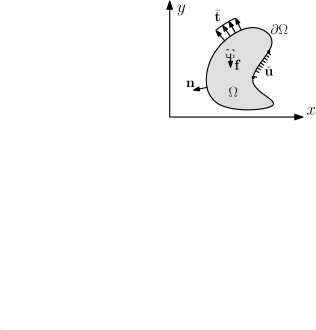
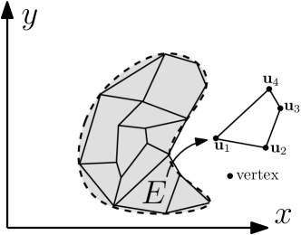
An example geometric domain of interest is provided in Figure 1a. Calculating field variables such as stress, strain, and displacements are the objective. By discretizing the domain with polygons, Figure 1b, it is then possible to use VEM. For VEM the polygons can be convex or non-convex with arbitrary number of sides. The interpolation space is necessarily populated with polynomial as well as non-polynomial functions as a consequence of selecting polygonal elements for discretization. The resulting polygon elements are able to compatibly interface with adjacent elements along their sides. Essentially, the polygon edges have polynomial interpolation functions, but polynomial plus (possibly) non-polynomial functions exist on the element interior. Nevertheless, it is only necessary to know polynomial functions along the edges to implement VEM. Consequently, the edge polynomials are chosen by selecting a polynomial order, . The present work chooses first order polynomials exclusively.
On element E, scalar-valued polynomials of order equal to or less are in the space . Consequently, is used to represent a 2D vector space of polynomials with two variables. The expression denotes a basis for the polynomial space. Illustrated below is a polynomial basis of order .
| (4) |
or
| (5) |
In equation (5), scaled monomials are used to create the components. The scaled monomials are defined as
| (6) |
where is the element centroid location and the diamter is (i.e., diameter of smallest circle that encloses all element vertices).
Remarks
-
(i)
It is possible to choose polynomials of higher order (see 8).
-
(ii)
Degrees of freedom are usually chosen by the analyst. For example, in this work each polygon vertex is chosen to include a displacement degree of freedom in the and direction. Clearly, each element edge has two vertices (points). A first order polynomial (a line) fits this condition. Then, values along element edges, for example, can be linearly interpolated.
-
(iii)
The number of terms in a polynomial base is equal to . For , . The number of terms in the polynomial base is 6.
-
(iv)
In (5), rigid body motion is provided by the first three monomials .
-
(v)
The number of vertices for a polygon, , is equivalent to the number of degrees of freedom, , in one spatial direction for a first order () VEM formulation.
2.3 Element Stiffness
Before the stiffness matrix is presented, it is necessary to define a variety of matrices and operators8, 9. To begin, recall that the modular matrix for plane stress is
| (7) |
and for plane strain is
| (8) |
where is Young’s modulus of elasticity, and is Poisson’s ratio.
Degree of Freedom Operator, . Define an operator, , which is found as follows: first, calculate polynomial vector evaluated at the vertex coordinates associated with dof , second, take the component of the vector that is directed along dof . The operator, , extracts the value of its argument, at dof , in the direction of dof , and the dofs (degrees of freedom) range from to .
The matrix. At coordinates of the degrees of freedom of polygon polynomial vector values are computed. These quantities are used to construct matrix . The result is
| (9) |
The engineering strain operator, . An engineering strain operator, , is applied to the polynomial basis as follows:
| (10) |
Acting on the polynomial base functions, the strain operator produces the matrix,
| (11) |
where in (11), represents the th (1st or 2nd) component for polynomial vector . For example, in 2D the polynomial vectors are shown in equations (4) and (5). Depending on the context, the strain operator has a specific use. For single vectors, like or , in 2D containing two components, the operator output is . For a group of vectors, like , as shown in (11), the operator output is , where for the first order polynomial base.
The engineering stress operator, . An engineering stress operator, , is obtained by matrix multiplication
| (12) |
In (12), the correct modular matrix, , for plane strain or plane stress is inserted. The engineering stress matrix is formed by using the results of (12)
| (13) |
The matrix. The matrix is formed, for rows to two columns at a time, for values ranging over vertex numbers to , according to the following formulas:
| (14) |

For equation (14), with reference to Figure 2, edge length is written as and the th edge outward unit normal vector components are . For vertex , edge length is the length from vertex to , where the polygon element has vertices, and normal is the outward unit normal to the edge from to . The terms or are dotted with the vector that arises from the right side of (14), as shown.
The matrix. The matrix is computed as
| (15) |
where
| (16) |
The matrix. A matrix is constructed by creating the matrix and then replacing the first three rows with the matrix. The infinitesimal strain, , is zero for of the polynomial basis, . It is for this reason that the beginning three rows of matrix given in (14) are populated with to create the matrix. If this was not done the first three rows would be zero (see 8, 9 for more details). Note, the matrix described herein should not be confused with the matrix 14 used with finite elements and incompressibility problems.
The projector matrix, . The projector matrix, , is constructed as
| (17) |
where
| (18) |
The 2D strain displacement matrix, . For 2D VEM the strain displacement matrix is written as
| (19) |
Engineering strain calculation, . Using the element vertex displacements, , the engineering strains are computed as shown below:
| (20) |
Remarks
-
(i)
The strains are ordered according to Voigt notation. The resulting strain vector contains the two-dimensional engineering strains , , . The size of the strain displacement matrix in (20) is .
-
(ii)
The standard displacement vector ordering is, .
-
(iii)
The formulation results in polygon elements with constant strains.
-
(iv)
The projection of the virtual element approximation, , onto the polynomial space is implied by the expression . The expression makes use of the projection operator .
Engineering stress calculation, . The stress terms needed to calculate the matrix are found by using equation (12). Yet, actual engineering stresses, calculated during post processing of elasticity problems, are found by using the applicable modular matrix and equation (20). The resulting formula for engineering stresses is
| (21) |
Element stiffness matrix, . Finally, analogous to finite element analysis, the element stiffness matrix for VEM is found found for each polygon element. The element stiffness for VEM is calculated from two contributions: a consistency part (23) and a stability part (24).
| (22) |
The consistency part is written as
| (23) |
where is the 2D plane stress or plane strain elastic modular matrix (see equations (7) and (8)), is the area of polygon element , and the polygon element has thickness .
The element stability stiffness part, given by Sukumar and Tupek 10, is given as
| (24) |
where the diagonal matrix is in size and is scaled as needed. The matrix has diagonal terms: , where in 2D, the modular matrix in 2D is the applicable case for plane strain or plane stress, and since elements are constructed from scaled monomials which create diameters on the order of 1, .
The above stability part of the element stiffness matrix is found to be effective for compressible materials in linear elasticity problems. It is also appropriate for plasticity problems. Later, in section 5, similar to Park et al.15, a stabilization matrix like (24) is provided for axisymmetric problems of near incompressibility.
2.4 Application of External Forces
Body forces and tractions impose external forces according to equation (3). Point loads at individual nodes (or vertices) of polygon elements are allowed also. Standard finite element methods are used to accomplish application of forces. The following linear form includes the three types of forces mentioned.
| (25) |
Mengolini et al. 8 provides additional discussion on the topic of load application. In the examples provided later, point loads or pressure loads are used. An external force vector, , is assembled from the point or pressure loads. Subsequently, the solution for nodal displacements is found by using the external force vector and the global stiffness. In anticipation of nonlinear problems, such as plasticity, equilibrium between external and internal forces is accomplished by use of a Newton-Raphson scheme.
2.5 Element Internal Forces
For nonlinear problems, in order to take advantage of an implicit analysis with iterations for equilibrium, local element internal forces are required. For plastic problems results from the stress integration process are used and a stabilization matrix adjustment is included. As a result, the internal forces for a single element are,
| (26) |
where for element the polygon area is , the engineering stress vector is , and is the latest incremental displacemen. Note that, for a particular time step in the nonlinear analysis, the stress vector is constant across the given element. Then, analogous to FEM, the global internal force vector is assembled from the individual element internal force vectors using the assembly operator 14. That is,
| (27) |
Remarks
-
(i)
An implicit nonlinear analysis is possible with the pieces provided above.
-
(ii)
The matrix in (22) is the individual element (tangent) stiffness. The global (tangent) stiffness matrix, , is assembled from the individual element (tangent) stiffnesses. It is important to recognize that, although this is similar to FEM, for VEM the number of degrees of freedom for a given element varies depending on the number of vertices in the polygon. Account of this must be made during assembly.
-
(iii)
Equation (27) expresses the global internal force vector, .
-
(iv)
Like FEM, according to the linear form (25), the global vector of external forces, , is created.
-
(v)
A residual, , for a given load or iteration step is now possible to create when nonlinear problems arise. The arc length control parameter is , and the residual vector used during equilibrium iterations is given by .
3 Mean Value Coordinates
As is seen in a later section, shape function values are needed at the centroid of each VEM element to create axisymmetric virtual elements. In the VEM formulation, recall that shape function values are not known on the interior of each polygonal element domain. As a result, a way to calculate the shape functions is needed. Several options are possible using the nodes of a particular polygon element. Moving least squares 16, maximum entropy 17, 18, and mean value coordinates (MVC) 19 shape functions are all possible solutions. The least costly, most robust, and easiest to implement are the mean value coordinates shape functions. They are an effective choice that maintains the benefits of VEM and the ability to handle convex as well as concave polygonal elements.
In Figure 3 an arbitrary polygon is shown. For an arbitrary point and having the polygon vertices , the shape function values (and derivatives) are obtained. As described by Floater 19, shape function values (and derivatives), , for each node are calculated as follows:
| (28) |
where
| (29) |
| (30) |
| (31) |
The following definitions apply for the above mean value coordinates formulas:
| (32) | ||||
| (33) | ||||
| (34) | ||||
| (35) | ||||
| for a vector | (36) |

4 The axisymmetric formulation
With the results of sections 2 and 3, the pieces necessary to construct axisymmetric VEM are in hand. A non-isoparametric formulation is presented since VEM and MVC shape functions are in global coordinates. For the following derivation, the vector of shape functions is denoted as .
4.1 Axisymmetric displacements
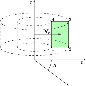
Consider Figure 4 with an axisymmetric element shown. The example element shown in the figure has an axisymmetric cross-section with 4 nodes. In general, the cross-section has an arbitrary polygonal cross-section with nodes to . For the cross-section the nodal displacements in the radial direction and direction are represented in terms of nodal shape functions as follows:
| (37) |
where and .
4.2 Axisymmetric cross-sectional strains
The 2D coordinates are relabeled in terms of the axisymmetric variables , . As a result, for a given element, the axisymmetric cross-sectional strains are expressed as
| (38) |
where the vector organizes and displacements as shown. Notice the strain displacement matrix, . Aside from coordinate direction relabeling, it is conceptually identical to the 2D elasticity VEM strain displacement matrix determined in section 2.3, equation (19). The shape functions themselves are not known, but the strain displacement matrix is computable from the VEM formulation.
4.3 The tangential or circumferential strain
For a given element in the VEM discretization, the tangential or circumferential strain is
| (39) |
where is the original circumference, is the final (or current) circumference, and is the distance from the axis of symmetry to the element centroid (see Figure 4), and the shape functions associated with tangential strain are evaluated at the element centroid coordinates. Note also that the strain displacement matrix requires shape function values. The shape function value are not available from the VEM formulation. Hence, an alternative means of calculating shape function values is needed. The mean value coordinates (MVC) shape functions of section 3 are used.
4.4 The axisymmetric strain displacement matrix
The strain displacement matrix for the axisymmetric case is constructed by combining the results from the in-plane case, , which comes from the VEM formulation, and the circumferential or tangential strain case, , which is constructed by using MVC shape functions. The result is the axisymmetric strain displacement matrix
| (40) |
4.5 Axisymmetric modular matrix and stresses
The axisymmetric modular matrix is
| (41) |
where .
The axisymmetric stresses are expressed as
| (42) |
5 Axisymmetric VEM - Elasticity
For problems of axisymmetric elasticity, using VEM notation, the consistent part of the element stiffness is expressed as
| (43) |
where the 2D element volume of is replaced with the axisymmetric volume, .
The stability part is expressed like the 2D elasticity case as
| (44) |
However, with an eye toward compressible and near incompressible problems, a procedure similar to 15, is used. Consequently, the diagonal matrix is defined to have diagonal terms: , where is the consistency matrix constructed with the part 14 of . That is
| (45) |
The element stiffness matrix is then formed in the usual way as
| (46) |
Special care is required to properly apply loads in axisymmetric problems. For an axisymmetric load at node the applied force is
| (47) |
where is the radial distance to node from the axis of symmetry, and is the load per unit distance along the circumference associated with . For an axisymmetric pressure at node the applied force is
| (48) |
where is the pressure, and is the distance along the surface tributary to node . For example, if the surface is parallel to the axis then , where is the coordinate of the node above and is the coordinate of the node below .
6 Axisymmetric VEM - Plasticity
Material nonlinearities like plasticity are easily included. For such a case, material properties must be updated during each load step. The local axisymmetric stiffness is the same as the case for elasticity except that a consistent elasto-plastic modular matrix, , is inserted into the expressions for and . Then the matrix becomes
| (49) |
As strains evolve during each load step, stresses and are updated according to the 3D plasticity formulation with radial return (see Simo and Taylor 20, and Simo and Hughes 21). The stabilization matrix here is a function of and is formed by taking the diagonal terms of the elasto-plastic consistency matrix, , according to the procedure for stabilization matrix (24) so that . All other formulas remain the same.
The internal force vector for an individual element is
| (50) |
where is the vector of element stresses obtained from the plasticity stress integration algorithm, and is the latest incremental displacement.
7 Numerical Implementation
For the nonlinear problems involving plasticity, implicit Newton-Raphson iterations are used with radial return at the constitutive level for each element. Global equilibrium is enforced by an arc-length path following scheme 22. As a result, the nonlinear analysis is carried out with typical ingredients: (i) a path following scheme (arc-length method), (ii) global external force vector, (iii) global internal force vector, and (iv) consistent global tangent stiffness matrix. For all example elasticity and plasticity problems the form of stabilization used is described by equations (44) and (49), respectively. All polygonal mesh generation is accomplished by using Polymesher 23.
8 Numerical Results
A variety of simulations are provided to illustrate the utility of the axisymmetric VEM. In particular, representative results of static elastic and plastic simulations, using consistent units, are provided. Results are compared to theoretical solutions or benchmark finite element solutions. For contour plots of stresses the calculated element stresses are used directly. For plots of stress versus radial distance, nodal stresses are shown and are calculated based on the average of element stresses common to a given node.
Convergence rates of axisymmetric VEM are computed using the displacement discrete error measure 24. The displacement error measure is calculated as
| (51) |
Consequently, the relative displacement error is calculated as
| (52) |
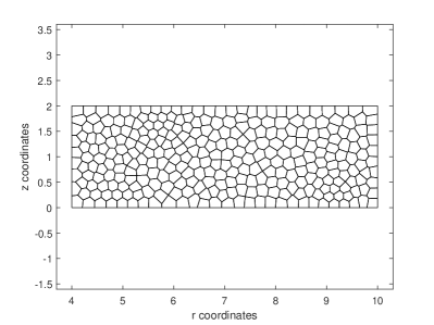
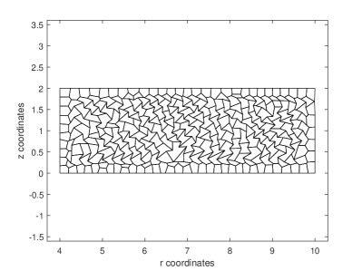
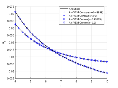
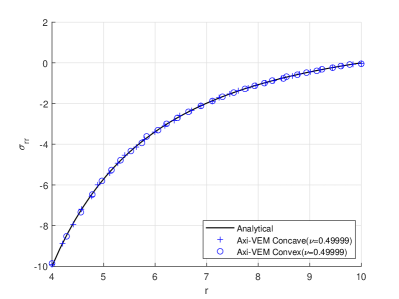
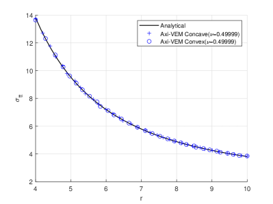
8.1 Cylinder Under Internal Pressure - Linear Elastic Lamé Problem, Case of Plane Strain
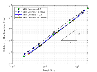
For the condition of plane strain a linear elastic cylinder is subject to internal pressure, . The cylinder has inner radius , and outer radius, . The modulus of elasticity and Poisson’s ratio or . Results are presented for the case of plane strain in the plane. Boundary conditions are set so that nodes at the top and bottom of the discretization are restrained in the direction causing everywhere. Plots for Figures 5abcde, are accomplished with 300 VEM elements. The theoretical solution 25, for radial displacements and stresses, is
| (53) |
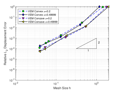
For problems of near incompressibility the results for Possion’s ratio equal to 0.49999 are handled without trouble. Convex and concave results are accomplished with indistinguishable results. The convergence characteristics shown in Figure 5f are within expected ranges for both compressible and near incompressible values of Poisson’s ratio and are not affected by concave or convex elements.
8.2 Sphere Under Internal Pressure - Linear Elastic Lamé Problem
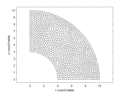
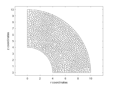
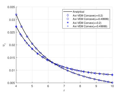
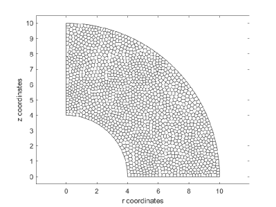
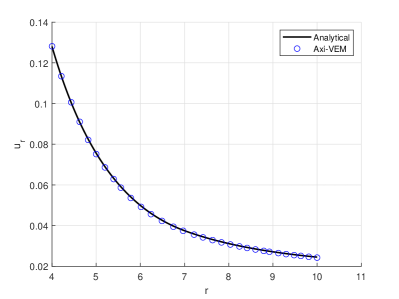
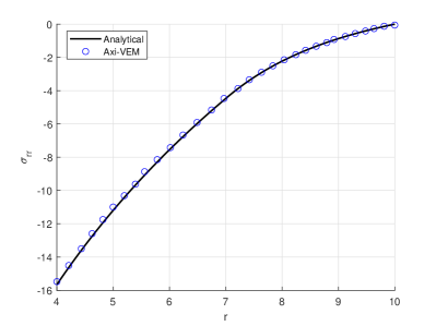
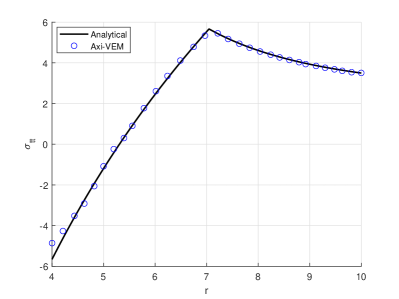
In Figures 6ab, the top half of an axisymmetric sphere is modeled with 1000 polygonal elements. The applied internal pressure is . The sphere internal radius , the external radius , modulus of elasticity , and Poisson’s ratio or . Vertical supports are provided at all nodes for which , and horizontal supports are provided at all nodes for which . The theoretical solution 25, for radial displacements and stresses, is
| (54) |
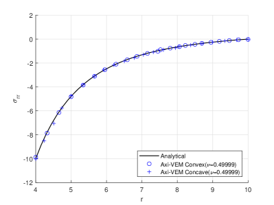
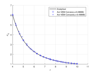
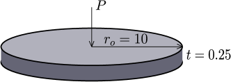
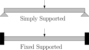
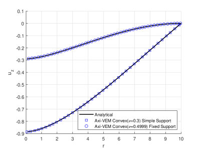
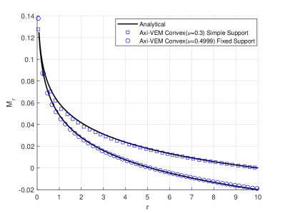
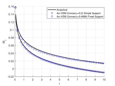
8.3 Elastic Circular Plate with Center Point Load
An elastic circular plate is loaded with a point load at the center, as shown in Figure 7a. The radius of the plate is . The plate has thickness and modulus of elasticity . Poisson’s ratio used in the various results are indicated in Figures 7cde. In particular, for some results Poisson’s ratios as high as 0.49999 are used to demonstrate that the formulation is not susceptible to locking for near incompressible problems. Results for displacements, radial moments, and tangential moments versus radial distance, , are shown to be in good agreement with analytical solutions. Furthermore, Figures 7cde illustrate results for plates with simply supported and fixed supported conditions. These problems are accomplished with an axisymmetric model using 18000 convex polygonal elements.
A study of normalized displacements and various Poisson ratios is provided in Table 1. For all results of the table, the circular plate is modeled with 9000 convex or mostly concave elements, as indicated. The results are in good agreement with the theoretical displacements which account for both bending and shear displacements. The axisymmetric VEM results have error of at most 3.76 % and for most cases less than 2%. The axisymmetric VEM formulation using concave or convex elements provides nearly indistinguishable results.
For the circular plate loaded by a point load at the center, the center displacement (bending plus shear) is , the radial moment is , and the tangential moment is . The theoretical solutions 26, 27 for an elastic circular plate with edges simply supported are
| (55) |
For the case of an elastic circular plate with edges fixed supported, the theoretical solutions 26, 27 are
| (56) |
| Simple Support | Fixed Support | |||
|---|---|---|---|---|
| Concave | Convex | Concave | Convex | |
| 0.0 | 0.9975 | 0.9982 | 0.9847 | 0.9858 |
| 0.3 | 0.9928 | 0.9932 | 0.9751 | 0.9749 |
| 0.49 | 0.9865 | 0.9875 | 0.9638 | 0.9641 |
| 0.499 | 0.9860 | 0.9870 | 0.9627 | 0.9631 |
| 0.49999 | 0.9863 | 0.9872 | 0.9624 | 0.9624 |
8.4 Elasto-Plastic Cylinder Under Internal Pressure
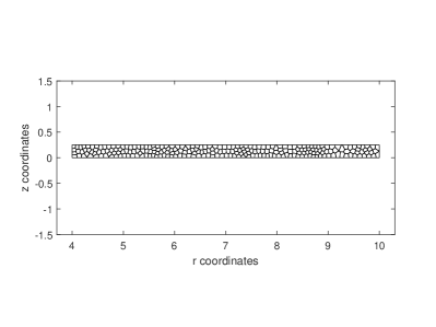
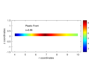
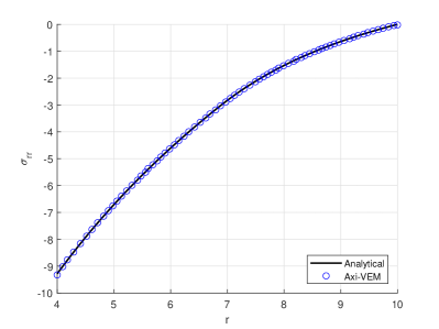
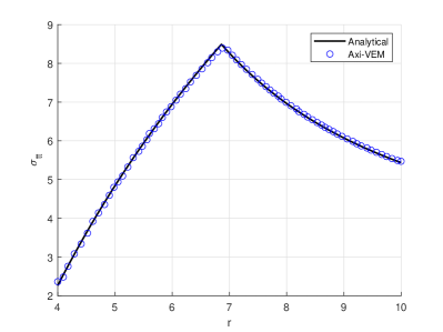
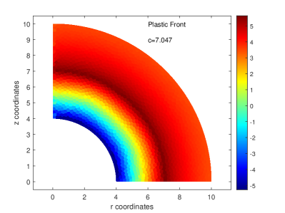
For the condition of plane strain an elasto-plastic cylinder with 250 convex elements (Figure 8a) is loaded by an internal pressure, . The cylinder has inner radius , and outer radius, . The modulus of elasticity , Poisson’s ratio is , the yield stress is , and for the case of perfect plasticity the hardening modulus is . When a cylinder begins to yield, the ‘plastic front’ location progresses from the inner radius toward the outer radius . Hence, for certain pressures, . For the case of pressure, , the plastic front is located at , which is in good agreement with the tangential stress results of Figures 8b and d. Radial stresses, versus radial coordinate, , are in good agreement with analytical results as shown in Figure 8c.
The theoretical solution of an elasto-plastic cylinder is given by Hill 28. Consider the pressure level associated with Figures 8bcd where the cylinder is yielded and the location of the plastic front, , is such that . For the elastic region, where , the theoretical solution is
| (57) |
For the plastic region, where , the theoretical solution is
| (58) |
For a given pressure (a function of c), the plastic front location, , is found numerically from the relation
| (59) |
8.5 Elasto-Plastic Sphere Under Internal Pressure
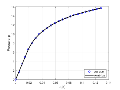
The top half of an elasto-plastic sphere is discretized with 1600 convex elements in Figure 9a. The discretization is provided with vertical supports for all nodes at and horizontal supports at all nodes . For the elastic-perfectly plastic sphere material, the modulus of elasticity , Poisson’s ratio , yield stress , and linear hardening modulus . The inner and outer radii of the sphere are and , respectively. A nonlinear analysis for the sphere up to a maximum pressure of is conducted. At the maximum pressure Figures 9bcd show plots for , , and versus radial coordinate, . A contour plot of tangential stresses is shown in Figure 9e. For the given maximum pressure, , the location of the plastic front, , is clearly visible in the contour plot and is in agreement with the predicted analytical value (also visible in plot (d)). For the nonlinear analysis a plot of pressure versus internal surface radial displacement is shown in Figure 9f. The plot is in excellent agreement with the analytically predicted pressure displacement curve.
The theoretical solution of an elasto-plastic sphere is given by Hill 28. Consider the pressure level associated with Figures 9bcde where the sphere is yielded and the location of the plastic front, , is such that . For the elastic region, where , the theoretical solution is
| (60) |
For the plastic region, where , the theoretical solution is
| (61) |
For a given pressure (a function of c), the plastic front location, , is found numerically from the relation
| (62) |
8.6 Elasto-Plastic Circular Plate Under Uniform Pressure
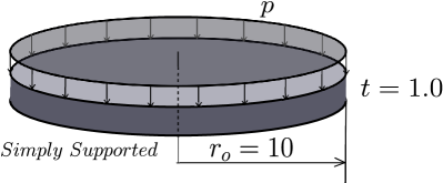
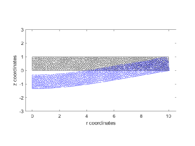
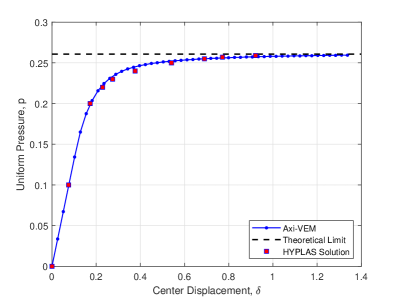
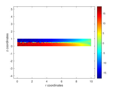
An elastic perfectly plastic simply supported circular plate is modeled with 900 convex polygonal elements. For the plate material, the modulus of elasticity , Poisson’s ratio , yield stress , and linear hardening modulus . The plate of radius and thickness is loaded downward with a uniform pressure. The relevant geometry, loading, discretization, and deflected shape are shown in Figures 10a and b. A nonlinear plot of pressure versus center displacement is provided in Figure 10c. The analysis limit pressure, , is in very good agreement with the theoretical limit pressure 29 . The nonlinear plot is substantially similar to finite element results achieved by the computer program HYPLAS developed by de Souza Neto et al 30. The progression of yielding along the radial direction of the plate is evident in the contour plot of radial stresses, , versus radial distance, , shown in Figure 10d.
9 Conclusions
In this paper, a first order axisymmetric VEM formulation for elasticity and elasto-plasticity is presented. This is accomplished by extending a 2D VEM formulation by adding an appropriately constructed row of mean value coordinates shape functions to the strain displacement matrix. By doing this, tangential strains, needed for axisymmetric problems, are included. The formulation is limited to small strains for elastic and plastic problems. Capabilities of the formulation are illustrated by solving example problems and comparing them to theoretical results or the results obtained by finite element solutions. For both elasticity and plasticity problems the formulation is able to easily obtain results that match the theoretical results. Several examples also show that near incompressibility is solved without volumetric locking. For the last problem presented, the axisymmetric VEM formulation with plasticity is able to produce results that are in very good agreement with a finite element solution. It is evident from the example problems that axisymmetric VEM is a viable method for solving axisymmetric solid mechanics problems.
All numerical methods have limitations. The formulation herein is no different and has typical limitations observed as follows: (a) need for suitable incremental step size in nonlinear analysis, particularly for plasticity problems, (b) need for adequate mesh refinement, (c) need for a robust polygon meshing scheme.
Suggested future work includes the following: (a) investigate the effect of stabilization free VEM, (b) incorporate finite strains.
Acknowledgements
LLY acknowledges the research support of Walla Walla University. Helpful discussions with Alejandro Ortiz-Bernardin are also gratefully acknowledged.
CONFLICT OF INTEREST STATEMENT
The authors declare no potential conflict of interests.
Data Availability Statement
The data that support the findings of this study are available from the corresponding author upon reasonable request.
References
- 1 Beirão da Veiga L, Brezzi F, Cangiani A, Manzini G, Marini LD, Russo A. Basic Principles of Virtual Element Methods. Mathematical Models and Methods in Applied Sciences 2013; 23(1): 199–214.
- 2 Beirão da Veiga L, Brezzi F, Marini LD, Russo A. The Hitchhiker’s Guide to the Virtual Element Method. Mathematical Models and Methods in Applied Sciences 2014; 24(8): 1541–1573.
- 3 Beirão da Veiga L, Brezzi F, Marini D. Virtual elements for linear elasticity problems. SIAM J Numer Analysis 2013; 51(12): 794–812.
- 4 Artioli E, Beirão da Veiga L, Lovadina C, Sacco E. Arbitrary order 2D virtual elements for polygonal meshes: Part I, elastic problem. Computational Mechanics 2017; 60(3): 355–377.
- 5 Taylor RL, Artioli E. VEM for Inelastic Solids. In: Oñate E. , ed. Advances in Computational Plasticity, Computational Methods in Applied Sciences 46. Switzerland: Springer. 2018 (pp. 381–394).
- 6 Artioli E, Beirão da Veiga L, Lovadina C, Sacco E. Arbitrary order 2D virtual elements for polygonal meshes: Part II, inelastic problem. Computational Mechanics 2017; 60(6): 643–657.
- 7 Beirão da Veiga L, Lovadina C, Mora D. A Virtual Element Method for elastic and inelastic problems on polytope meshes. Computer Methods in Applied Mechanics and Engineering 2015; 295(10): 327–346.
- 8 Mengolini M, Benedetto MF, Aragón AM. An engineering perspective to the virtual element method and its interplay with the standard finite element method. Computer Methods in Applied Mechanics and Engineering 2019; 350: 995–1023.
- 9 Yaw LL. Introduction to the Virtual Element Method for 2D Elasticity. arXiv: 2301.11928v2 [math.NA] 2023.
- 10 Sukumar N, Tupek MR. Virtual elements on agglomerated finite elements to increase the critical time step in elastodynamic simulations. International Journal for Numerical Methods in Engineering 2022; 123: 4702–4725.
- 11 Flanagan D, Belytschko T. A uniform strain hexahedron and quadrilateral with orthogonal hourglass control. International Journal for Numerical Methods in Engineering 1981; 17: 679–706.
- 12 Russo A, Sukumar N. Quantitative study of the stabilization parameter in the virtual element method. arXiv:2304.00063 [math.NA] 2023.
- 13 Cangiani A, Manzini G, Russo A, Sukumar N. Hourglass stabilization and the virtual element method. International Journal for Numerical Methods in Engineering 2015; 102: 404-436.
- 14 Hughes TJR. The Finite Element Method - Linear Static and Dynamic Finite Element Analysis. Mineola, NY: Dover. 1st ed. 2000.
- 15 Park K, Chi H, Paulino G. B-bar virtual element method for nearly incompressible and compressible materials. Meccanica 2021; 56: 1423–1439.
- 16 Belytschko T, Krongauz Y, Organ D, Fleming M, Krysl P. Meshless Methods: An Overview and Recent Developments. Computer Methods in Applied Mechanics and Engineering 1996; 139: 3–47.
- 17 Sukumar N. Construction of polygonal interpolants: A maximum entropy approach. International Journal for Numerical Methods in Engineering 2004; 61(12): 2159–2181.
- 18 Sukumar N, Wright RW. Overview and construction of meshfree basis functions: From moving least squares to entropy approximants. International Journal for Numerical Methods in Engineering 2007; 70(2): 181–205.
- 19 Floater MS. Generalized barycentric coordinates and applications. Acta Numerica 2015; 24: 161–214.
- 20 Simo JC, Taylor RL. Consistent Tangent Operators For Rate-Independent Elastoplasticity. Computer Methods in Applied Mechanics and Engineering 1985; 48: 101–118.
- 21 Simo JC, Hughes TJR. Computational Inelasticity. New York: Springer-Verlag . 1998.
- 22 Crisfield MA. Non-linear Finite Element Analysis of Solids and Structures – Vol 1. Chichester, England: John Wiley & Sons Ltd. . 1991.
- 23 Talischi C, Paulino GH, Pereira A, Menezes IFM. PolyMesher: a general-purpose mesh generator for polygonal elements written in Matlab. Structural and Multidisciplinary Optimization 2012; 45: 309–328.
- 24 Chen A, Sukumar N. Stress-hybrid virtual element method on quadrilateral meshes for compressible and nearly-incompressible linear elasticity. International Journal for Numerical Methods in Engineering November 1, 2023.
- 25 Timoshenko SP, Goodier JN. Theory of Elasticity. New York: McGraw-Hill. 2nd ed. 1951.
- 26 Timoshenko SP, Woinowsky-Krieger S. Theory of Plates and Shells. New York: McGraw-Hill. 2nd ed. 1959.
- 27 Ugural AC. Stresses in Plates and Shells. New York: McGraw-Hill . 1981.
- 28 Hill R. The mathematical theory of plasticity. Oxford, UK: Clarendon Press. 1st ed. 1950.
- 29 Skrzypek JJ, Hetnarski RB. Plasticity and Creep. Boca Raton, FL: CRC Press . 1993.
- 30 de Souza Neto EA, Perić D, Owen DRJ. Computational Methods for Plasticity. Chichester, UK: John Wiley & Sons Ltd. . 2008.