Backward Stability of Explicit External Deflation for the Symmetric Eigenvalue Problem
Abstract
A thorough backward stability analysis of Hotelling’s deflation, an explicit external deflation procedure through low-rank updates for computing many eigenpairs of a symmetric matrix, is presented. Computable upper bounds of the loss of the orthogonality of the computed eigenvectors and the symmetric backward error norm of the computed eigenpairs are derived. Sufficient conditions for the backward stability of the explicit external deflation procedure are revealed. Based on these theoretical results, the strategy for achieving numerical backward stability by dynamically selecting the shifts is proposed. Numerical results are presented to corroborate the theoretical analysis and to demonstrate the stability of the procedure for computing many eigenpairs of large symmetric matrices arising from applications.
1 Introduction
Let be an real symmetric matrix with ordered eigenvalues , and the corresponding eigenvectors . Let be an interval containing the eigenvalues at the lower end of the spectrum of . We are interested in computing the partial eigenvalue decomposition
| (1.1) |
where , and . We are particularly interested in the case where the interval is of the width , and may contain a large number of eigenvalues of .
A majority of subspace projection methods for computing the partial eigenvalue decomposition (1.1), such as the Lanczos methods [13, 1], typically converge first to the eigenvalues on the periphery of the spectrum. A projection subspace of a large dimension is necessary to compute the eigenvalues located deep inside the spectrum. Maintaining the orthogonality of a large projection subspace is computationally expensive. To reduce the dimensions of projection subspaces and accelerate the convergence, a number of techniques such as the restarting [17, 8, 20] and the filtering [11] have been developed.
This paper revisits a classical deflation technique known as Hotelling’s deflation [6, 19, 13]. Hotelling’s deflation computes the partial eigenvalue decomposition (1.1) through a sequence of low-rank updates. In the simplest case, supposing that the lowest eigenpair of is computed by an eigensolver, by choosing a real shift and defining the rank-one update matrix
the eigenpair of is displaced to an eigenpair of , while all the other eigenpairs of and are the same. If the shift , then the eigenpair is shifted outside the interval and the eigenpair of becomes the lowest eigenpair of . Subsequently, we can use the eigensolver again to compute the lowest eigenpair of . The procedure is repeated until all the eigenvalues in the interval are found. Since the low-rank update of the original can be done outside of the eigensolver, we refer to this strategy as an explicit external deflation (EED) procedure, to distinguish from the deflation techniques used inside an eigensolver, such as TRLan [20] and ARPACK [9]. Recently the EED has been combined with Krylov subspace methods to progressively compute the eigenpairs toward the interior of the spectrum of symmetric eigenvalue problems [12, 21], and extended to structured eigenvalue problems [2, 3].
In the presence of finite precision arithmetic, the EED procedure is susceptible to numerical instability due to the accumulation of numerical errors from previous computations; see, e.g., [19, p. 585] and [15, p. 96]. In [13, Chap. 5.1], Parlett showed that the change to the smallest eigenvalue in magnitude by deflating out the largest computed eigenvalue would be at the same order of the round-off error incurred. In [14], for nonsymmetric matrices, Saad derived an upper bound on the backward error norm and showed that the stability is determined by the angle between the computed eigenvectors and the deflated subspace. Saad concluded that “if the angle between the computed eigenvector and the previous invariant subspace is small at every step, the process may quickly become unstable. On the other hand, if this is not the case then the process is quite safe, for small number of requested eigenvalues.”
However, none of the existing studies had examined the effect of the choice of shifts on the numerical stability. In this paper, we present a thorough backward stability analysis of the EED procedure. We first derive governing equations of the EED procedure in the presence of finite precision arithmetic, and then derive upper bounds of the loss of the orthogonality of the computed eigenvectors and the symmetric backward error norm of the computed eigenpairs. From these upper bounds, under mild assumptions, we conclude that the EED procedure is backward stable if the shifts are dynamically chosen such that (i) the spectral gaps, defined as the separation between the computed eigenvalues and shifted ones, are maintained at the same order of the norm of the matrix , and (ii) the shift-gap ratios, defined as the ratios between the largest shift in magnitude and the spectral gaps, are at the order of one. Our analysis implies that the re-orthogonalization of computed eigenvectors and the large angles between the computed eigenvectors and the previous invariant subspaces are unnecessary. Based on theoretical analysis, we provide a practical shift selection scheme to guarantee the backward stability. For a set of test matrices from applications, we demonstrate that the EED in combination with an established eigensolver can compute a large number of eigenvalues with backward stability.
The rest of the paper is organized as follows. In Section 2, we present the governing equations of the EED in finite precision arithmetic. In Section 3, we derive the upper bounds on the loss of orthogonality of computed eigenvectors and the symmetric backward error norm of computed eigenpairs. From these upper bounds, we derive conditions for the backward stability of the EED procedure. In Section 4, we discuss how to properly choose the shifts to satisfy the stability conditions and outline an algorithm for combining the EED procedure with an eigensolver. Numerical results to verify the sharpness of the upper bounds and to demonstrate the backward stability of the EED for symmetric eigenvalue problems from applications are presented in Section 5. Concluding remarks are given in section 6.
Following the convention of matrix computations, we use the upper case letters for matrices and the lower case letters for vectors. In particular, we use for the identity matrix of dimension . If not specified, the dimensions of matrices and vectors conform to the dimensions used in the context. We use for transpose, and and for -norm and the Frobenius norm, respectively. The range of a matrix is denoted by . We also use to denote the minimal singular values of a matrix. Other notations will be explained as used.
2 EED in finite precision arithmetic
Suppose that we use an established eigensolver called EIGSOL, such as TRLan [20] and ARPACK [9], to successfully compute the lowest eigenpair of with
where and the residual vector satisfies
| (2.1) |
for a prescribed convergence tolerance . The EED procedure starts with computing the lowest eigenpair of by EIGSOL satisfying
where , and the residual vector satisfies (2.1). At the first EED step, we choose a shift and define
By choosing the shift , the lowest eigenpair of is an approximation of the second eigenpair of . Subsequently, we use EIGSOL to compute the lowest eigenpair of satisfying
where the residual vector satisfies (2.1). Meanwhile, expressing the computed eigenpair in terms of , we have
Proceeding to the second EED step, we choose a shift and define
where and . By choosing the shift , the lowest eigenpair of is an approximation of the third eigenpair of . Then we use EIGSOL again to compute the lowest eigenpair of satisfying
where the residual vector satisfies (2.1). Meanwhile, expressing the computed eigenpairs and in terms of , we have
where , , and is the strictly lower triangular part of the matrix , i.e., .
In general, at the -th EED step, we choose a shift and define
| (2.2) |
where and with . Then by choosing the shift , the lowest eigenpair of is an approximation of the -th eigenpair of . We use EIGSOL to compute the lowest eigenpair of satisfying
| (2.3) |
where and the residual vector satisfies (2.1), i.e.,
| (2.4) |
Meanwhile, for the computed eigenpairs in terms of , we have
| (2.5) |
and for the computed eigenpairs with in terms of , we have
| (2.8) |
where and .
Combining (2.5) and (2.8), we have
| (2.9) |
where , , is the strictly lower triangular part of the matrix and . Eqs. (2.3) and (2.9) are referred to as the governing equations of steps of (inexact) EED procedure.
For the backward stability analysis of the EED procedure, we introduce the following two quantities associated with the shifts for a -step EED:
-
•
the spectral gap of , defined as the separation between the computed eigenvalues and the shifted ones:
(2.10) where , the set of computed eigenvalues, and , the set of computed eigenvalues after shifting (see Figure 1 for an illustration);
Figure 1: Illustration of the spectral gap -
•
the shift-gap ratio, defined as the ratio of the largest shift and the spectral gap :
(2.11)
We will see that and are crucial quantities to characterize the backward stability of the EED procedure.
3 Backward stability analysis of EED
In this section, we first review the notion of backward stability for the computed eigenpairs. Then we derive upper bounds on the loss of orthogonality of computed eigenvectors and the backward error norm of computed eigenpairs by the EED procedure, and reveal conditions for the backward stability of the procedure.
3.1 Notion of backward stability
By the well-established notion of backward stability analysis in numerical linear algebra [5, 18], the following two quantities measure the accuracy of the approximate eigenpairs of computed by the EED procedure:
-
•
the loss of orthogonality of the computed eigenvectors ,
(3.1) -
•
the symmetric backward error norm of the computed eigenpairs ,
(3.2) where is the set of the symmetric backward errors for the orthonormal basis from the polar decomposition111The polar decomposition of a matrix is given by where is orthonormal and is symmetric positive semi-definite. of , namely,
(3.3)
For a prescribed tolerance of the stopping criterion (2.4) for an eigensolver EIGSOL, the EED procedure is considered to be backward stable if
| (3.4) |
and
| (3.5) |
where the constants in the big-O notations are low-degree polynomials in the number of the EED steps.
3.2 Loss of orthogonality
We first prove the following lemma to reveal the structure of the orthogonality between the computed eigenvectors.
Lemma 3.1.
By the governing equations (2.3) and (2.9) of steps of EED, if , then for , the matrices and are non-singular, and
| (3.6) |
Furthermore,
-
(i)
,
-
(ii)
,
where and are the spectral gap and the shift-gap ratio defined in (2.10) and (2.11), respectively, and is the loss of the orthogonality defined in (3.1).
Proof.
By the governing equations (2.3) and (2.9) of steps of EED, for , we have
and
Consequently,
| (3.7) |
where is a diagonal matrix.
By the definition (2.10) of the spectral gap ,
| (3.8) |
Hence the matrix is non-singular and the bound (i) holds.
Next we exploit the structure of the product to derive a computable upper bound on the loss of orthogonality of computed eigenvectors .
Theorem 3.1.
Proof.
By the definition (3.1), we have
| (3.11) |
Recall Lemma 3.1 that, for any ,
Hence we can derive from (3.11) that
| (3.12) |
Since
we arrive at
| (3.13) |
Letting , where , then the inequality (3.13) is recast as
| (3.14) |
By the fact that the quadratic polynomial in (3.14) is concave, we conclude that
This proves the upper bound in (3.10). ∎
Remark 3.1.
A straightforward way to derive an upper bound of is to use the relation
and the following bound from Lemma 3.1
However, this would lead to a pessimistic upper bound of . In contrast, in Theorem 3.1, we exploit the structure of the orthogonality to obtain a tighter bound (3.10) of . Eq. (3.12) in the proof is the key step. In Example 5.1 in Section 5, we will demonstrate numerically that the bound (3.10) is indeed a tight upper bound on the loss of orthogonality .
3.3 Symmetric backward error norm
In this section, we derive a computable upper bound on the symmetric backward error norm of computed eigenpairs of defined in (3.2). First, the following lemma gives an upper bound of the norm of the residual for :
| (3.15) |
Lemma 3.2.
Proof.
From the governing equation (2.9) of the EED procedure after steps, we have
| (3.17) |
On the other hand, by the definition (2.2) of , we have
| (3.18) |
Combining (3.17) and (3.18), we obtain the residual
| (3.19) |
Consequently, the norm of the residual is bounded by
| (3.20) |
Note that and is the strictly upper triangular part of the matrix , and we have
| (3.21) |
where, for the third inequality, we again use the fact that by the definition of the loss of orthogonality . Left-multiplying (3.13) by , we know that
Plugging into (3.21), we obtain
Combine with (3.20) and we arrive at the upper bound (3.16) of . ∎
Now we recall the following theorem by Sun [18].
Theorem 3.2 (Thm.3.1 in [18]).
Let be approximate eigenpairs of a symmetric matrix . Let be the orthonormal basis from the polar decomposition of . Define the set
| (3.22) |
Then is non-empty and there exists a unique such that
| (3.23) |
where is the residual and is the orthogonal projection onto the orthogonal complement of .
From Lemma 3.2 and Theorem 3.2, we have the following computable upper bound on the symmetric backward error norm of the computed eigenpairs of .
Theorem 3.3.
Proof.
For the computed eigenvectors of , let be the orthonormal basis from the polar decomposition of , and the set be defined in (3.3). It follows from the definition (3.2) and Theorem 3.2 that
| (3.25) |
where is the residual of defined in (3.15), and is the orthogonal projection onto the orthogonal complement of the subspace , i.e.,
By the equation (3.19), . Hence we have
| (3.26) |
On the other hand, by the definition (3.1) of and the assumption , we have
which implies the following lower bound of the singular value
| (3.27) |
Plug (3.26) and (3.27) into (3.25) and recall the upper bound of in Lemma 3.2, and then we obtain
where the second inequality is due to . This completes the proof. ∎
3.4 Backward stability of EED
In Theorems 3.1 and 3.3, the upper bounds (3.10) and (3.24) for and involve the quantity from the previous EED step. In this section, under a mild assumption, we derive explicit upper bounds for and , and then reveal conditions for the backward stability of the EED procedure.
Lemma 3.3.
Proof.
First observe that by the definitions (2.10) and (2.11), is monotonically decreasing with the index and is monotonically increasing with . Therefore, the assumption (3.28) implies the inequalities
| (3.32) |
Since the stopping criterion (2.4) of EIGSOL implies
| (3.33) |
inequalities (3.32) leads to
| (3.34) |
(i) We prove the inequality (3.29) by induction. To begin with, recall that , which implies , , and . Hence (3.29) holds for . Now, for , assume that and . Since , we can apply Theorem 3.1 and derive from (3.10) that
| (3.35) |
where the last inequality of (3.35) is by and (3.34). This implies immediately
Therefore, (3.29) follows by induction.
(ii) Since we have and by (3.29), we can apply Theorem 3.1 and derive from (3.10) that
| (3.36) |
where in the second inequality we used and the first inequality in (3.34). Recall the error bound of from (3.33) and we obtain (3.30).
(iii) We have and by (3.29). It also follows from (3.36) and (3.34) that . Therefore, we can apply Theorem 3.3 and derive from (3.24) that
where in second inequality we used . Since by definition (2.11), we can relax the leading constant as . Recall the error bound of from (3.33) and we prove (3.31). ∎
By the error bounds (3.30) and (3.31) in Lemma 3.3, we can see that the quantities and play important roles for the stability of the EED procedure. A sufficient condition to achieve the backward stability (3.4) and (3.5) is given by and . In summary, we have the following theorem for the backward stability of the EED procedure.
Theorem 3.4.
We note that when the shifts are dynamically chosen such that the conditions (3.37) are satisfied, the assumption of the inequality (3.28) is indeed mild.
Remark 3.3.
From the upper bound (3.30) of the loss of orthogonality , we see that if the spectral gap is too small, i.e., , then could be amplified by a factor of . On the other hand, from the upper bound (3.31) of the symmetric backward error norm , we see that when is too large, i.e., , could be amplified by a factor of . We will demonstrate these observations numerically in Example 5.2 in Section 5.
4 EED in practice
In Section 3.4, we derived the required conditions (3.37) of the spectral gap and the shift-gap ratio for the backward stability of the EED procedure. The quantities and are controlled by the selection of the shifts . In this section, we discuss a practical selection scheme of the shifts to satisfy the conditions (3.37), and then present an algorithm that combines an eigensolver EIGSOL with the EED procedure to compute eigenvalues in a prescribed interval .
4.1 Choice of the shifts
We consider the following choice of the shift at the -th EED step,
| (4.1) |
where is a parameter with . The shifting scheme (4.1) has been used in several previous works, although without elaboration on the choice of parameter ; see [13, Chap.5.1] and [12, 21]. In the following, we will discuss how to choose the parameter such that the conditions (3.37) can hold.
To begin with, the choice of the shifts in (4.1) implies that the spectral gap in (2.10) satisfies
| (4.2) |
where and . On the other hand, it also implies that the shift-gap ratio in (2.11) satisfies
| (4.3) |
Now recall that and the computed eigenvalues , for , so we have
Hence, (4.2) and (4.3) lead to
| (4.4) |
where
The problem is then turned to the choice of parameter such that the quantities and to satisfy the conditions (3.37).
Let us consider a frequently encountered case in practice where the width of the interval satisfies
Then by setting
we have
and
Consequently, by (4.4), the spectral gap and the shift-gap ratio satisfy the desired conditions (3.37).
In summary, for the EED procedure in practice, we recommend the use of the following strategy for the choice of the shift at the -th EED,
| (4.5) |
to compute the eigenvalues in an interval , where .
4.2 Algorithm
An eigensolver EIGSOL combined with the EED procedure to compute the eigenvalues in an interval at the lower end of the spectrum of is summarized in Algorithm 1.
A few remarks are in order:
-
•
In practice, we never need to form the matrix at step 6 explicitly. We can assume that the only operation that is required by EIGSOL is the matrix-vector product .
- •
-
•
At step 8, an ideal validation method is to use the inertias of the shifted matrix . However, computation of the inertias is a prohibitive cost for large matrices. An empirical validation is to monitor the lowest eigenvalue of . All eigenpairs in the interval are considered to be found when is outside the interval .
5 Numerical experiments
In this section, we first use synthetic examples to verify the sharpness of the upper bounds (3.10) and (3.24) on the loss of orthogonality and the symmetric backward error norm of the EED procedure under the choice (4.5) of the shifts . We present the cases where improper choices of the shifts may lead to numerical instability of the EED procedure. Then we demonstrate the numerical stability of the EED procedure for a set of large sparse symmetric matrices arising from applications.
We use TRLan as the eigensolver. TRLan is a C implementation of the thick-restart Lanczos method with adaptive sizes of the projection subspace [20, 22, 23]. The convergence criterion of an approximate eigenpair is the residual norm satisfying
where is a user-specified tolerance and Anorm is a -norm estimate of computed by TRLan. The starting vector is a random vector.
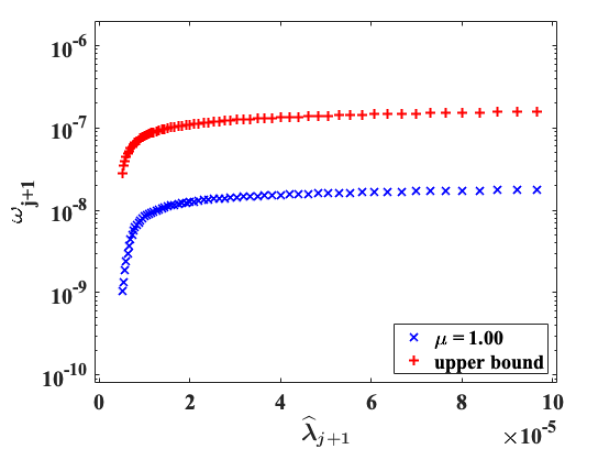
Example 5.1.
In this example, we demonstrate the sharpness of the upper bounds (3.10) and (3.24) on the loss of orthogonality and the symmetric backward error norm with the choice (4.5) of the shifts .
We consider a diagonal matrix with diagonal elements
where and the matrix size . The spectrum range of is . The eigenvalues of are clustered around and . We are interested in computing the eigenvalues in the interval . The computed -norm of is .
To closely observe the convergence, TRLan is slightly modified so that the convergence test is performed at each Lanczos iteration. The maximal dimension of the projection subspace is set to be .
Numerical results of TRLan with the EED procedure for computing all the eigenvalues in the interval are summarized in Table 1, where the 4th column is the loss of orthogonality , the 5th column is the upper bound (3.10) of , the 6th column is the residual norm and the 7th column is the upper bound (3.24) of . Note that here we use the quantities and interchangeably as discussed in Remark 3.2.
From Table 1, we observe that with the choice (4.5) of the shifts , and . Therefore, the conditions (3.37) of the spectral gap and the shift-gap ratio for the backward stability are satisfied. Consequently, the loss of orthogonality of the computed eigenvectors is and the symmetric backward error norm of the computed eigenpairs is . In addition, we observe that the upper bounds (3.10) and (3.24) of and are tight within an order of magnitude.
| bound (3.10) | bound (3.24) | |||||
|---|---|---|---|---|---|---|
| 1.00 | ||||||
| 1.00 | ||||||
| 1.00 |
Example 5.2.
In this example we illustrate that improperly chosen shifts may lead to instability of the EED procedure.
In Remark 3.3, we stated that if the shifts are chosen such that the spectral gaps are too small, i.e., , then the loss of orthogonality of the computed eigenvectors could be amplified by a factor of . Here is an example using the same diagonal matrix in Example 5.1. The combination of TRLan and EED is used to compute the eigenvalues in the interval . Let us set the shifts with , which is much smaller than the recommended value of . Numerical results are summarized in Table 2, where the tolerance for TRLan. We observe that , and the loss of orthogonality of the computed eigenvectors is indeed amplified by a factor of . We note that since , the symmetric backward error norms .
| bound (3.10) | bound (3.24) | |||||
|---|---|---|---|---|---|---|
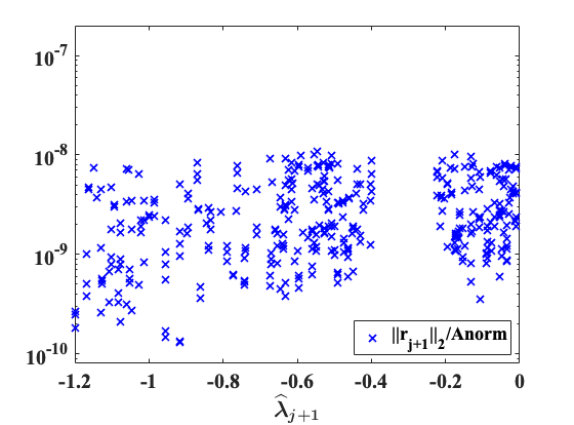
In Remark 3.3, we also stated that if the shifts are chosen such that the shift-gap ratios are too large, then the symmetric backward error norm could be amplified by a factor of . Here is an example. We flip the sign of the diagonal elements of defined in Example 5.1, and set . We compute eigenvalues in the interval using TRLan with EED procedure. The computed -norm of is .
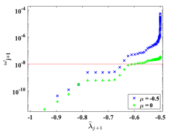
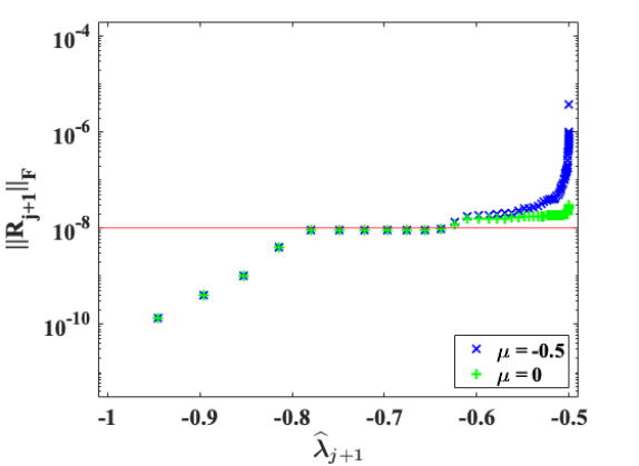
Instead of the choice (4.5) for the shifts , we set with . The blue -lines in Figure 3 are the loss of orthogonality and the residual norms for the computed eigenpairs for . As we observe that for the first computed eigenvalues in the subinterval of , since the spectral gap and the shift-gap ratio , the computed eigenpairs are backward stable with and . However, for the computed eigenvalues in the subinterval of , the computed eigenpairs are not backward stable due to the facts that the spectral gaps become small, , and the shift-gap ratios grows up to . Consequently, the loss of orthogonality and the residual norm are increased by a factor of up to , respectively. The stability are restored if the shifts are chosen according to the recommendation (4.5) as shown by the green -lines in Figure 3.
Example 5.3.
In this example, we demonstrate the numerical stability of TRLan with the EED procedure for a set of large sparse symmetric matrices from applications.
The statistics of the matrices are summarized in Table 3, where is the size of the matrix, nnz is the number of nonzero entries of the matrix, is the spectrum range, and is the number of eigenvalues in the interval . The quantities are calculated by computing the inertias of the shifted matrices . The Laplacian is the negative 2D Laplacian on a -by- grids with Dirichlet boundary condition [16]. The worms20 is the graph Laplacian worms20_10NN in machine learning datasets [4]. The SiO, Si34H36, Ge87H76 and Ge99H100 are Hamiltonian matrices from PARSEC collection [4].
| matrix | nnz | ||||
|---|---|---|---|---|---|
| Laplacian | |||||
| worms20 | |||||
| SiO | |||||
| Si34H36 | |||||
| Ge87H76 | |||||
| Ge99H100 |
We run TRLan with a maximal number of Lanczos vectors to compute the lowest eigenpairs of the matrix . The convergence test is performed at each restart of TRLan. All the converged eigenvalues in the interval are shifted by EED. Meanwhile, we also keep a maximal number of the lowest unconverged eigenvectors as the starting vectors of TRLan for the matrix . All the eigenvalues in are assumed to be computed when the lowest converged eigenvalue is outside the interval . This combination of TRLan is referred to as TRLED.
TRLED is compiled using the icc compiler (version 2021.1)
with the optimization flag -O2,
and linked to BLAS and LAPACK available in Intel Math Kernel Library
(version 2021.1.1). The experiments are conducted on a MacBook
with GHz Intel Core i5 CPU and 8GB of RAM.
For numerical experiments, we set the maximal number of Lanczos vectors . When starting TRLED for , the maximal number of the starting vectors is . The convergence tolerance for the residual norm was set to as a common practice for solving large scale eigenvalue problems with double precision; see for example [11].
Numerical results of TRLED are summarized in Table 4, where the 2nd column is the number of the computed eigenpairs in the interval , the 3rd column is the number of steps of EED performed, the 4th column is the loss of orthogonality , and the 5th column is the relative residual norm of the computed eigenpairs . From the quantities in Table 3 and in Table 4, we see that for all test matrices the eigenvalues in the prescribed intervals are successfully computed with the desired backward stability.
| matrix | CPU time (sec.) | |||||
|---|---|---|---|---|---|---|
| TRLED | TRLan | |||||
| Laplacian | ||||||
| worms20 | ||||||
| SiO | ||||||
| Si34H36 | ||||||
| Ge87H76 | ||||||
| Ge99H100 | ||||||
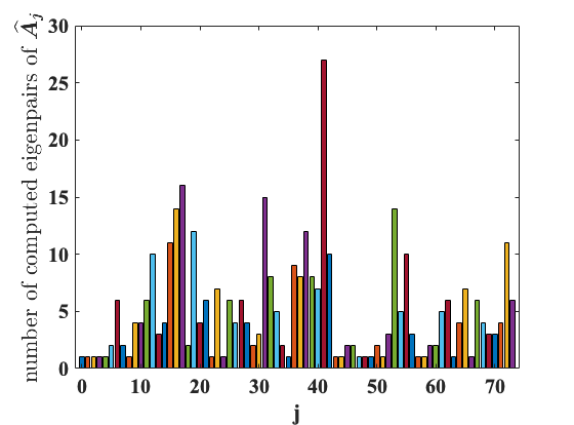
The left plot of Figure 4 is a profile of the number of converged eigenvalues at each external deflation of a total of 74 EEDs for the matrix Ge99H100. The right plot of Figure 4 shows the relative residual norms of all 372 computed eigenpairs in the interval. We observe that a large number of converged eigenvalues are deflated and shifted away at some EED steps.
To examine whether the multiple explicit external deflations lead to
a significant increase in execution time, in the 6th and 7th columns
of Table 4, we record the CPU time of TRLED and TRLan
for computing all eigenvalues in the same intervals.
For TRLan, we set the maximal number of Lanczos vectors to
. The restart scheme with restart=1 is used.
TRLan is compiled and executed under the same setting as TRLED.
We observe comparable execution time of TRLED and TRLan.
In fact, TRLED is slightly faster.
We think this might be
due to the facts that TRLED uses fewer Lanczos vectors,
which compensates the cost of the matrix-vector products
and the warm start with
those unconverged eigenvectors from the previous deflated matrix
. These are subjects of future study.
6 Concluding remarks
Based on the governing equations of the EED procedure in finite precision arithmetic, we derived the upper bounds on the loss of the orthogonality of the computed eigenvectors and the symmetric backward error norm of the computed eigenpairs in terms of two key quantities, namely the spectral gaps and the shift-gap ratios. Consequently, we revealed the required conditions of these two key quantities for the backward stability of the EED procedure. We present a practical strategy on the dynamically selection of the shifts such that the spectral gaps and the shift-gap ratios satisfy the required conditions.
There are a number of topics that can be explored further. One of them is the acceleration effect of the warm starting the EIGSOL with the unconverged eigenvectors of for computing of the lowest eigenpairs of . Another one is how to efficiently perform the matrix-vector products in EIGSOL by exploiting the sparse plus low rank structure of the matrix . Communication-avoid algorithms for sparse-plus-low-rank matrix-vector products can be found in [10, 7]. A preliminary numerical study for high performance computing is reported in [21].
References
- [1] Z. Bai, J. Demmel, J. Dongarra, A. Ruhe, and H. van der Vorst. Templates for the Solution of Algebraic Eigenvalue Problems: A Practical Guide. SIAM, Philadelphia, PA, 2000.
- [2] Z. Bai, R.-C. Li, and W. Lin. Linear response eigenvalue problem solved by extended locally optimal preconditioned conjugate gradient methods. Sci. China Math., 259:1443–1460, 2016.
- [3] P.-Y. Chen, B. Zhang, and M. Al Hasan. Incremental eigenpair computation for graph laplacian matrices: theory and applications. Social Network Analysis and Mining, 8(1):4, 2018.
- [4] T. Davis and Y. Hu. The University of Florida sparse matrix collection. ACM Trans. Math. Software (TOMS), 38(1):1–25, 2011.
- [5] D. Higham and N. Higham. Structured backward error and condition of generalized eigenvalue problems. SIAM J. Mat. Anal. Appl., 20(2):493–512, 1998.
- [6] H. Hotelling. Analysis of a complex of statistical variables into principal components. J. of Educational Psychology, 24(6):417, 1933.
- [7] N. Knight, E. Carson, and J. Demmel. Exploiting data sparsity in parallel matrix powers computations. In the proceedings of the international conference on parallel processing and applied mathematics (PPAM), 2014.
- [8] R. Lehoucq and D. Sorensen. Deflation techniques for an implicitly restarted Arnoldi iteration. SIAM J. Matrix Anal. Appl., 17(4):789–821, 1996.
- [9] R. Lehoucq, D. Sorensen, and C. Yang. ARPACK Users’ Guide: Solution of Large-Scale Eigenvalue Problems with Implicitly Restarted Arnoldi Methods. SIAM, Philadelphia, PA, 1998.
- [10] C. Leiserson, S. Rao, and S. Toledo. Efficient out-of-core algorithms for linear relaxation using blocking covers. J. Comput. Syst. Sci. Int., 54:332––344, 1997.
- [11] R. Li, Y. Xi, E. Vecharynskio, C. Yang, and Y. Saad. A thick-restart Lanczos algorithm with polynomial filtering for Hermitian eigenvalue problems. SIAM J. Sci. Comput., 38:A2512–A2534, 2016.
- [12] J. Money and Q. Ye. Algorithm 845: EIGIFP: a MATLAB program for solving large symmetric generalized eigenvalue problems. ACM Trans. Math. Software (TOMS), 31(2):270–279, 2005.
- [13] B. N. Parlett. The Symmetric Eigenvalue Problem. SIAM, Philadelphia, PA, 1998.
- [14] Y. Saad. Numerical solution of large nonsymmetric eigenvalue problems. Comput. Phys. Commun., 53(1-3):71–90, 1989.
- [15] Y. Saad. Numerical Methods for Large Eigenvalue Problems: revised edition, volume 66. SIAM, Philadelphia, PA, 2011.
- [16] B. Smith and A. Knyazev. Laplacian in 1D, 2D or 3D, 2015 (accessed March 24, 2020). https://www.mathworks.com/matlabcentral/fileexchange/27279-laplacian-in-1d-2d-or-3d.
- [17] Danny C Sorensen. Implicit application of polynomial filters in a -step Arnoldi method. SIAM J. Matrix. Anal. Appl., 13(1):357–385, 1992.
- [18] J.-G. Sun. A note on backward perturbations for the Hermitian eigenvalue problem. BIT Numer. Math., 35(3):385–393, 1995.
- [19] J. H. Wilkinson. The algebraic eigenvalue problem. Clarendon Press, Oxford, 1965.
- [20] K. Wu and H. Simon. Thick-restart Lanczos method for large symmetric eigenvalue problems. SIAM J. Matrix Anal. Appl., 22(2):602–616, 2000.
- [21] I. Yamazaki, Z. Bai, D. Lu, and J. Dongarra. Matrix powers kernels for thick-restart Lanczos with explicit external deflation. In 2019 IEEE International Parallel Distributed Processing Symposium (IPDPS), pages 472–481. IEEE, 2019.
- [22] I. Yamazaki, Z. Bai, H. Simon, L.-W. Wang, and K. Wu. Adaptive projection subspace dimension for the thick-restart Lanczos method. ACM Trans. Math. Software (TOMS), 37(3):27, 2010.
- [23] I. Yamazaki, K. Wu, and H. Simon. nu-TRLan User Guide. Technical report, LBNL-1288E, 2008. Software https://codeforge.lbl.gov/projects/trlan/.