Bad semidefinite programs: they all look the same
Abstract
Conic linear programs, among them semidefinite programs, often behave pathologically: the optimal values of the primal and dual programs may differ, and may not be attained. We present a novel analysis of these pathological behaviors. We call a conic linear system badly behaved if the value of is finite but the dual program has no solution with the same value for some We describe simple and intuitive geometric characterizations of badly behaved conic linear systems. Our main motivation is the striking similarity of badly behaved semidefinite systems in the literature; we characterize such systems by certain excluded matrices, which are easy to spot in all published examples.
We show how to transform semidefinite systems into a canonical form, which allows us to easily verify whether they are badly behaved. We prove several other structural results about badly behaved semidefinite systems; for example, we show that they are in in the real number model of computing. As a byproduct, we prove that all linear maps that act on symmetric matrices can be brought into a canonical form; this canonical form allows us to easily check whether the image of the semidefinite cone under the given linear map is closed.
Key words: conic linear programming; semidefinite programming; duality; closedness of the linear image of a closed convex cone; pathological semidefinite programs
MSC 2010 subject classification: Primary: 90C46, 49N15; secondary: 52A40
OR/MS subject classification: Primary: convexity; secondary: programming-nonlinear-theory
1 Introduction
Many problems in engineering, combinatorial optimization, machine learning, and related fields can be formulated as the primal-dual pair of conic linear programs
where is a linear map between finite dimensional Euclidean spaces and is its adjoint, is a closed, convex cone, is its dual cone, and means Note that the subscript refers to the objective of the primal problem.
Problems and generalize linear programs and share some of the duality theory of linear programming. For instance, a pair of feasible solutions always satisfies the weak duality inequality However, in conic linear programming pathological phenomena occur: the optimal values of and of may differ, and they may not be attained.
In particular, semidefinite programs (SDPs) and second order conic programs (SOCPs) — probably the most useful and pervasive conic linear programs — often behave pathologically: for a variety of examples we refer to the textbooks [6, 37, 11, 3, 42] surveys [44, 41, 27] and research papers [34, 1, 43]. Pathological conic LPs are both theoretically interesting and often difficult, or impossible to solve numerically.
These pathologies arise, since the linear image of a closed convex cone is not always closed. For recent studies about when such sets are closed (or not), see e.g., [4, 2, 29]. Three approaches (which we review in detail below) can help to avoid or remedy the pathologies: one can impose a constraint qualification (CQ), such as Slater’s condition; one can regularize using a facial reduction algorithm [16, 46, 31]; or write an extended dual [34, 24], which uses extra variables and constraints. However, such CQs often do not hold, and neither facial reduction algorithms nor extended duals can help solve all pathological instances.
We started this research observing that pathological SDPs in the literature look curiously similar and one of our main goals is to find the root cause of the similarity. We focus on the system underlying and call
| () |
badly behaved if there exists such that either does not attain its value or its value differs from the value of We call () well behaved if it is not badly behaved.
Main contributions of the paper:
-
(1)
In Theorem 1 of Section 2 we characterize when the system () is badly or well behaved. At the heart of Theorem 1 is a simple geometric condition that involves the set of feasible directions at i.e.,
In Theorem 1 we unify two well-known (and seemingly unrelated) conditions for () to be well behaved: the first is Slater’s condition, and the second requires to be polyhedral.
-
(2)
In Section 3 we characterize when a semidefinite system
() is badly behaved via certain excluded matrices. We assume (with no loss of generality) that a maximum rank positive semidefinite matrix of the form is
(1.1) We prove (in Theorem 2) that () is badly behaved iff there is a matrix which is a linear combination of the and of the form
(1.2) where is is positive semidefinite, and Here stands for rangespace.
The excluded matrices and are easy to spot in all published badly behaved semidefinite systems (we counted about in the above references). The simplest such system is
(1.3) where is any real number: in (1.3) the right hand side serves as and the matrix on the left hand side serves as
Theorem 3 similarly characterizes well behaved semidefinite systems.
-
(3)
How do we verify that () is badly or well behaved? In other words, how do we convince a nonexpert reader that an instance of () is badly or well behaved? Theorems 4 and 5 in Section 4 show how to transform () into an equivalent standard system, whose bad or good behavior is self-evident. The transformation is surprisingly simple, as it relies mostly on elementary row operations — the same operations that are used in Gaussian elimination. A natural analogy (and our inspiration) is how one transforms an infeasible linear system of equations to derive the obviously infeasible equation
Here we also prove that i) badly/well behaved semidefinite systems are in in the real number model of computing ii) for a well behaved semidefinite system we can restrict optimal dual matrices to be block-diagonal, and iii) roughly speaking, we can partition a well behaved system into a strictly feasible part, and a linear part.
As a byproduct, we prove that all linear maps that act on symmetric matrices can be brought into a canonical form; this canonical form allows us to easily check whether the image of the semidefinite cone under the given linear map is closed.
- (4)
-
(5)
Since most examples in the main body of the paper have at most three variables and matrices, in Appendix A we give a larger illustrative example with four variables and matrices. We prove other technical results in Appendix B.
We illustrate our results by many examples. The only technical proofs in the main body of the paper are those of Theorem 1 and of Lemma 5, and these can be safely skipped at first reading.
Related work A fundamental question in convex analysis is whether the linear image of a closed convex cone is closed. In this paper we rely on Theorem 1.1 from [29], which we summmarize in Lemma 1. This result gives several necessary conditions, and exact characterizations for the class of nice cones. We refer to Bauschke and Borwein [4] for the closedness of the continuous image of a closed convex cone; to Auslender [2] for the closedness of the linear image of an arbitrary closed convex set; and to Waksman and Epelman [47] for another related result. For perturbation results we refer to Borwein and Moors [13, 14]; the latter paper shows that the set of linear maps under which the image of a closed convex cone is not closed is small both in terms of measure and category. For a more general problem, whether the intersection of an infinite sequence of nested sets is nonempty, Bertsekas and Tseng [7] gave a sufficient condition. Their characterization is in terms of a certain retractiveness property of the set sequence.
We say that is a strong dual of if they have the same value, and attains this value, when it is finite. Thus in general is not a strong dual of Using this terminology, () is well behaved exactly if is a strong dual of for all We say that () satisfies Slater’s condition, if there is such that is in the relative interior of if this condition holds, then () is well behaved.
Ramana in [34] proposed a strong dual for SDPs, which uses polynomially many extra variables and constraints. His result implies that semidefinite feasibility is in in the real number model of computing. Klep and Schweighofer in [24] constructed a Ramana-type strong dual for SDPs, which, interestingly, is based on ideas from algebraic geometry, rather than from convex analysis.
The facial reduction algorithm of Borwein and Wolkowicz in [16, 15] converts () into a system that satisfies Slater’s condition, and is hence well behaved. The algorithm relies on a sequence of reduction steps. For more recent, simplified facial reduction algorithms, see Waki and Muramatsu [46] and Pataki [31]. Ramana, Tunçel, and Wolkowicz in [36] proved the correctness of Ramana’s dual from the facial reduction algorithm of [16, 15], showing the connection of these two seemingly unrelated concepts. We refer to Ramana and Freund [35] for a proof that the Lagrange dual of Ramana’s dual has the same value as the original problem. Generalizations of Ramana’s dual are known for conic LPs over nice cones [31]; and for conic LPs over homogeneous cones (Pólik and Terlaky [33]).
For a generalization of the concept of strict complementarity (a concept that plays an important role in our work), we refer to Pena and Roshchina [32]. Schurr et al in [40] characterize universal duality — when strong duality holds for all right hand sides and objective functions. Tunçel and Wolkowicz in [43] related the lack of strict complementarity in a homogeneous conic linear system to the existence of an objective function with a positive gap.
We finally remark that the technique of reformulating equality constrained SDPs (relying mostly on elementary row operations), to easily verify their infeasibility was used recently by Liu and Pataki [25].
1.1 Preliminaries. When is the linear image of a closed convex cone closed?
We now review some basics in convex analysis, relying mainly on references [38, 23, 12, 5]. In Lemma 1 we also give a short and transparent summary of a result on the closedness of the linear image of a closed convex cone from [29].
If and are elements of the same Euclidean space, we sometimes write for For a set we denote its linear span, the orthogonal complement of its linear span, its closure, and interior by and respectively. For a convex set we denote its relative interior by For a convex set and we define
| (1.4) | |||||
| (1.5) | |||||
| (1.6) |
Here is the set of feasible directions at in and is the tangent space at in
A set is a cone if holds for all and Let be a closed convex cone. Its dual cone is
For a convex subset of we say that is a face of if and implies that and are in
For and we say that is strictly complementary to if If is the semidefinite cone, or the second order cone, then is strictly complementary to iff is strictly complementary to in other cones, however, this may not be the case (see a discussion in [28]).
We say that a closed convex cone is nice, if
We know that polyhedral, semidefinite, and -order cones are nice [16, 15, 29]; the intersection of a nice cone with a linear subspace and the linear preimage of a nice cone are nice [18]; hence homogeneous cones are nice, as they are the intersection of a semidefinite cone with a linear subspace (see [17, 22]). In [30] we characterized nice cones, proved that they must be facially exposed and conjectured that all facially exposed cones are nice. However, Roshchina [39] disproved this conjecture.
We denote the rangespace, nullspace, and adjoint operator of a linear operator by and respectively. We denote by the set of by symmetric matrices, and by the set of symmetric positive semidefinite (psd) matrices. For symmetric matrices and we write [] to denote that is positive semidefinite [positive definite], and we write to denote the trace of We have with respect to the inner product.
We will use the fact that for an affine subspace
For and an invertible matrix we will use the identity
| (1.7) |
For matrices and we let
and for sets of matrices and we define
For instance, (where the order of the matrix will be clear from context) is the set of matrices with the upper left block positive semidefinite and the rest of the components zero.
We write for the identity matrix of order
The following question is fundamental in convex analysis: when is the linear image of a closed convex cone closed? We state and illustrate a short version of Theorem 1.1 from [29], which gives easily checkable conditions which are “almost” necessary and sufficient. We will use Lemma 1 later on to prove Theorem 1.
Lemma 1.
∎
Our first example which illustrates Lemma 1 is very simple:
Example 1.
Let and define the map as
Then and is not closed: a direct computation shows where stands for the set of strictly positive reals.
The next, more involved example illustrates the key point of Lemma 1: the image set usually has much more complicated geometry than and Lemma 1 sheds light on the geometry of via the geometry of the simpler set
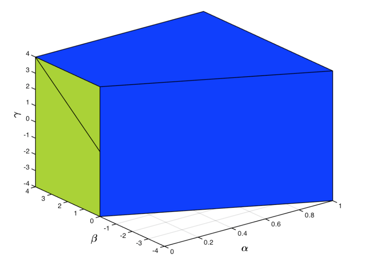
Example 2.
Let and define the map as
Thus where
It is a straightforward computation (which we omit) to show
| (1.8) |
The set is shown on Figure 1 in blue, and in green. (Note that the blue diagonal segment on the green facet actually belongs to )
2 When is a conic linear system badly or well behaved?
In this section we present our main characterization of when () is badly or well behaved (these concepts are defined in the Introduction). We first need a definition.
Definition 1.
We start with a basic lemma:
∎
To put Lemma 2 into perspective, note that the image set in Lemma 2 is closed if is closed (one can argue this directly or by modifying the proof of Lemma 2). In turn, if is closed, then the duality gap between and is zero, even if lives in an infinite dimensional space — see, e.g., Theorem 7.2 in [3] (where our primal is called the dual). The proof of Lemma 2 is standard, and we give it in Appendix B.
The main result of this section follows (recall the definition of and related sets from (1.4)–(1.6)). We write for the rangespace of the operator
Theorem 1.
∎
To build intuition we show how Theorem 1 unifies two classical, seemingly unrelated, sufficient conditions for () to be well-behaved.
Corollary 1.
Proof Let be a maximum slack in (). If is polyhedral, then so is . If () satisfies Slater’s condition, then clearly so In both cases is closed, hence Condition (1) holds, so () is well behaved. ∎
Though Lemma 2 is a bit simpler to state than Theorem 1, the latter will be more useful. On the one hand, Lemma 2 relies on the closedness of the linear image of which may not be easy to check. On the other hand, Theorem 1 relies on the geometry of the cone itself, and not on the geometry of its linear image. The geometry of typical cones that occur in optimization — e.g. the geometry of the semidefinite cone — is well understood. Thus Theorem 1, among other things, will lead to a proof that badly behaved semidefinite systems are in in the real number model of computing. Lemma 2, by itself, affords no such corollary.
Note that if , then by Lemma 2 the system () is well behaved iff is closed. Thus in this case Lemma 1 and Theorem 1 are equivalent. To prove the general case of Theorem 1 we use a homogenization argument.
To prove the Claim we first note that if is a maximum slack in () and is some other slack, then is also a maximum slack for all (by Theorem 6.1 in [38]). A similar result holds for ().
Now let be a maximum slack in (), then is a slack in (). Next, let be a maximum slack in (). By the properties of the relative interior, and since is a slack in (), we have that is a slack in () for some So must hold, and (after normalizing) we can assume Hence is a slack in () and
will do. This completes the proof of the claim.
To proceed with the proof of the theorem, we note that the set of maximum slacks in () is a relatively open set, so by Theorem 18.2 in [38] it is contained in where is some face of Therefore for any maximum slack (see e.g. Lemma 2.7 in [28]) so the sets and depend only on Hence we are free to use any maximum slack of () in our proof, and we will use the particular maximum slack provided in the preceding Claim.
For convenience we define the linear map
which corresponds to the homogenized conic linear system ().
We first note that (trivially)
Equations (1.4)–(1.6) imply that the same statement holds, if we replace the operator by or
Hence the following equations hold:
| (2.9) | |||||
| (2.10) |
Consider now the following variants of conditions (1) and (2):
-
-
There is strictly complementary to and
Since is a maximum slack in (), we have Hence by Lemma 1 with we find
and that equivalence holds when is nice.
We next note that by (2.9) condition is equivalent to (1). Also, if is as specified in then
and since both terms above are nonnegative, we must have Thus using (2.10) we find that statement is equivalent to condition (2) in Theorem 1. Thus we have
with equivalence holding when is nice. Finally, is nice if and only if is, thus invoking Lemma 2 completes the proof. ∎
We can easily modify the proof of Theorem 1 to show that conditions 1 and 2 suffice for () to be well behaved, even under a weaker condition than being nice: it is enough for to be closed, where is the smallest face of that contains This more general version of Theorem 1 implies that Corollary 1 holds even if we do not assume that is nice – we refer the interested reader to version 3 of the paper on arxiv.org.
3 When is a semidefinite system badly or well behaved?
We now specialize the results of Section 2, and characterize when the semidefinite system () is badly or well behaved. To this end, we consider the primal-dual pair of SDPs
where and are scalars.
Specializing Definition 1 to the semidefinite system (), we find that i) a slack in () is a matrix of the form and ii) a maximum slack in () is a maximum rank slack. We also note that the cone of positive semidefinite matrices is nice [16, 15, 29].
We make the following
We can easily satisfy Assumption 1, at least from a theoretical point of view, as follows. If is any maximum rank slack in (), is a matrix of suitably scaled eigenvectors of and we apply the rotation to all and then the maximum rank slack in the rotated system is in the required form. (We do not make a claim about actually computing or ; we discuss this point more at the end of Section 4 ).
In the interest of the reader we first state and illustrate the main results, then prove them.
Theorem 2.
Example 3.
In the problem
| (3.13) |
the only feasible solution is The dual program, in which we denote the components of by is equivalent to
which has a infimum but does not attain it.
The certificates of the bad behavior of the system in (3.13) are
Example 4.
The problem
| (3.14) |
again has an attained supremum. The reader can easily check that the value of the dual program is (and it is attained), so there is a finite, positive duality gap.
We next characterize well behaved semidefinite systems:
Theorem 3.
Example 5.
Example 6.
This example illustrates both badly and well behaved semidefinite systems, depending on the value of the parameter
| (3.18) |
Let us write for the constraint matrices on the left, and for the right hand side matrix in (3.18). We first observe that is the maximum rank slack; indeed i) so it is a slack, and ii) the matrix
| (3.19) |
satisfies for all Hence is orthogonal to any slack matrix, so the rank of any slack matrix is at most
We return to Examples 3–6 in Section 4. As we will see there, the bad or good behavior of semidefinite systems can be verified using only an elementary linear algebraic argument, without ever referring to Theorems 2 or 3. We will use Examples 3–6 as illustrations.
The reader may find it interesting to spot the and excluded matrices in other pathological SDPs in the literature, e.g., in the instances in [6, 11, 3, 44, 41, 34, 43, 27].
Theorems 2 and 3 simply follow from Theorem 1 and from Lemma 3 below, which describes the set of feasible directions and related sets in the semidefinite cone:
Lemma 3.
∎
The proof of Lemma 3 is given in Appendix B.
Proof of Theorem 2 By condition (1) of Theorem 1 we see that () is badly behaved, iff there is a matrix such that
Thus our result follows from parts (3.21) and (3.23) in Lemma 3. ∎
Proof of Theorem 3 We apply Theorem 1 to the system (). We first observe that a matrix is strictly complementary to if and only if
Next we note that the first part of condition in Theorem 1 holds iff there is such a that satisfies (3.16). By (3.20) and (3.22) in Lemma 3 the second part of condition (2) in Theorem 1 holds iff all which are of the form
satisfy This completes the proof. ∎
We note that for semidefinite systems that are strictly feasible, a matrix similar to the matrix in Theorem 2 can make sure that the optimal primal-dual solution pair fails strict complementarity; see [48].
Although we focus on feasible systems, we obtain natural corollaries about weakly infeasible SDPs, a class of pathological infeasible SDPs. To describe the connection, note that the alternative system
| (3.24) |
gives a natural proof of infeasibility of (): if (3.24) is feasible, then () is trivially infeasible. However, () and (3.24) may both be infeasible, in which case we call the semidefinite system () weakly infeasible.
As background on weakly infeasible SDPs, we mention that Waki [45] recently described a method for generating weakly infeasible SDPs based on Lasserre’s relaxation for polynomial optimization problems; Klep and Schweighofer [24] analyzed weakly infeasible SDPs using real algebraic geometry techniques; and Lourenco et al [26] proved that any weakly infeasible SDP with order matrices has a weakly infeasible subsystem with dimension at most
To apply our machinery to weakly infeasible SDPs, we homogenize () to obtain the system
| (3.25) |
Assume that the system (3.25) satisfies Assumption 1. First, suppose that () is weakly infeasible. Then (3.25) is badly behaved, since
| (3.26) |
but there is no solution feasible in the dual of (3.26) (such a dual solution would be feasible in (3.24)). Hence by Theorem 2 the excluded matrices and appear in (3.25). In turn, if (3.25) satisfies the conditions of Theorem 3 and hence it is well behaved, then () cannot be weakly infeasible.
4 Reformulations. Badly behaved semidefinite systems are in
4.1 Reformulations
To motivate the discussion of this section, we recall a basic result from the theory of linear equations:
-
“The system is infeasible if and only if its row echelon form contains the equation where ”
Since the ”if” direction is trivial, we will — informally — say that the row echelon form is an easy-to-verify certificate, or witness, of infeasibility.
In this section we describe analogous results for a very different problem : we show how to transform () into an equivalent system whose bad or good behavior is trivial to verify. As a corollary we prove that badly (and well) behaved semidefinite systems are in in the real number model of computing. (In this model we can store arbitrary real numbers in unit space and perform arithmetic operations in unit time; see e.g. [9]. We do not claim that badly behaved semidefinite systems are in i.e., we do not provide a polynomial time algorithm to decide whether () is badly behaved. We discuss this point in more detail at the end of this section.)
Definition 2.
We obtain an elementary reformulation, or simply a reformulation, of by a sequence of the following operations:
-
(1)
Apply a rotation to all and where and is invertible.
-
(2)
Replace by where
-
(3)
Exchange and where
-
(4)
Replace by where
We obtain an elementary reformulation of the system () by applying the preceding operations with some
Where do these operations come from? Operations (3) and (4) are equivalent to elementary row operations (inherited from Gaussian elimination) done on
Proof Operations (1)-(4) of Definition 2 keep the value of finite, if it is finite; and infinite, if it is infinite. Suppose now that is feasible in with value, say, and we apply operations (1) and (2) with rotation matrix and vector Then identity (1.7) implies that is feasible in the dual of the reformulated problem with value Operations (3) and (4) preserve the feasibility and objective value of a solution of Thus if () is well behaved, so are its reformulations, and this completes the proof of the ”Only if” direction. Since () is a reformulation of its reformulations, the ”If” direction follows as well. ∎
4.2 Reformulating () to verify maximality of the maximum rank slack
Recall that is the maximum rank slack in () described in Assumption 1. We reformulate () in two steps. In the first step, given in Lemma 5, we reformulate () so the resulting system has easy-to-verify witnesses that is a maximum rank slack. (The matrices in Lemma 5 will be the witnesses.)
In Lemma 5 we rely on a facial reduction algorithm (see [16, 15, 46, 31]). It is important that in Lemma 5 we only use rotations, i.e., type (1) operations of Definition 2.
Lemma 5.
∎
If i.e., () satisfies Slater’s condition, then we just take for all and in Lemma 5.
To build intuition, we first establish why the matrices indeed prove that the rank of any slack matrix is at most Let be a slack in (), and as in the statement of Lemma 5. Then for some So and hence the last rows and columns of are zero; and imply that the next rows and columns of are zero, and so on. Inductively we find that the last rows and columns of are zero, hence must have rank at most
Thus we can prove that is a maximum rank slack in () (hence also in ()) using
-
(1)
a vector such that and
-
(2)
the matrices of Lemma 5.
We next illustrate Lemma 5.
Example 7.
(Examples 3, 4, 5 and 6 continued) In all these examples it is easy to show why the maximum rank slack is indeed a slack. Also, in Example 3
is orthogonal to all constraint matrices (using the inner product), so it proves that the rank of any slack matrix is at most one.
In Example 4 the matrix proves that the rank of any slack is at most one, and in Example 5 the matrix proves that the rank of any slack is at most two. (So the first three examples do not even need to be reformulated to have a convenient proof that is a maximum rank slack.)
In Example 6 we let
and apply the rotation to all matrices to obtain the system
| (4.29) |
Now is orthogonal to all constraint matrices in (4.29), and this proves that the rank of any slack is at most one, so is a maximum rank slack.
In Appendix A we give a larger example, in which we need two matrices to prove that any slack matrix has rank at most
Proof of Lemma 5
To find the reformulation assume that we have a reformulation of the form () and matrices such that (4.28) holds for all and for At the start and for all For brevity, let We claim that
This indeed follows since if is a slack in () then (using the same argument that we used before) the last rows and columns of must be zero.
If we set and stop; otherwise, we define the cone Clearly, and its dual cone are of the form
Next, define the affine subspace
Since is also a maximum rank slack in , and we have hence by a classic theorem of the alternative (see e.g. Lemma 1 in [31]).
Let
Since we have
for some (Again, the symbols stand for submatrices with arbitrary elements). Let be the number of positive eigenvalues of since we have
Let be an invertible matrix such that and We apply the rotation to and the rotation to all and to
By (1.7) the equation (4.28) holds for all and for By the form of now are in the required shape (see equation (4.27)). We then set and continue.
Clearly, our algorithm terminates in finitely many steps, so the proof is complete. ∎
4.3 Reformulating () to verify that it is badly behaved
In Theorem 4 we give the final reformulation of () to prove its bad behavior. We point out that in Theorem 4 the proof of the ”if” direction is elementary, thus the reformulated system () is an easy-to-verify certificate that () is badly behaved.
Theorem 4.
The system () is badly behaved if and only if it has a reformulation
| () |
where
-
(1)
matrix is the maximum rank slack, and its maximality can be verified by matrices as given by Lemma 5.
-
(2)
The matrices
are linearly independent.
-
(3)
Proof (If) By Lemma 4 it is enough to prove that () is badly behaved. Let be feasible in with a corresponding slack Note that the last rows and columns of must be zero, otherwise would be a slack with larger rank than Hence, by condition (2) we must have Next, let us consider the SDP
| (4.30) |
which, by the above argument, has optimal value We prove that its dual cannot have a feasible solution with value so suppose that
is such a solution. By we get hence by psdness of we deduce Thus
which contradicts the assumption that is feasible in the dual of (4.30).
Proof (Only if) We start with the system () given by Lemma 5 and further reformulate it. For brevity we denote the constraint matrices on the left hand side by throughout the process.
We first replace by in (). Since the resulting system is still badly behaved, by Theorem 2 there is a matrix of the form
with By the form of we can assume (otherwise we can replace by ).
Note that the block of comprising the last columns must be nonzero. We pick an such that replace by then switch and Next we choose a maximal subset of the matrices so their blocks comprising the last columns are linearly independent. We let to be one of these matrices (this can be done, since is now the certificate matrix), and permute the so this special subset becomes for some
We finally add suitable multiples of to to zero out the last columns and rows of the latter, and arrive at the required reformulation. ∎
Example 8.
(Examples 3, 4 and 6 continued) The first two of these examples are already in the standard form (). Suppose now in Example 6, i.e., the system (3.18) is badly behaved. Recall that by a rotation we brought (3.18) to the simpler form (4.29). Then in (4.29) we set
and obtain the system
| (4.31) |
which is in the standard form () (with ). The objective function yields a zero optimal value over (4.31) but there is no dual solution with the same value: we can argue this as in the proof of the ”if” direction in Theorem 4.
Note that the certificate matrix of Theorem 2 appears in the system () as the last matrix on the left hand side.
4.4 Reformulating () to verify that it is well behaved
We now turn to well behaved semidefinite systems, and in Theorem 5 we show how to reformulate them to easily verify their good behavior. In Theorem 5 we also show block-diagonality of dual optimal solutions. Note that the proof of the ”if” direction in Theorem 5 is easy, so the system () is an easy-to-verify certificate of good behavior.
Theorem 5.
Proof (If and block-diagonality) Let be such that
| (4.32) |
is finite. By the proof of Lemma 4 it suffices to prove that the dual of (4.32) has a block-diagonal solution with value An argument like in the proof of Theorem 4 proves that holds for any feasible in (4.32), so
| (4.33) |
Since (4.33) satisfies Slater’s condition, there is feasible in its dual with
As the are linearly independent, we can choose (which is possibly not psd) such that
satisfies the equality constraints of the dual of (4.32). We then add a positive multiple of the identity to to make psd. Taking condition (3) into account we can see that after this operation is feasible in the dual of (4.32) and clearly holds. The proof is now complete.
Proof (Only if) We again start with the system () that Lemma 5 provides; now () is well behaved. (We also note that the matrix of Theorem 3 became the matrix of Lemma 5, after we rotated it.) We first replace by Next we choose a maximal subset of the whose lower principal blocks are linearly independent. We permute the if needed, to make this subset for some
To complete the process we add multiples of to to zero out the lower principal block of the latter. By Theorem 3 the upper right block of and the symmetric counterpart also become zero. This concludes the proof. ∎
Example 9.
We next discuss some implications of Theorem 5. First, as the proof of the ”if” direction shows, we can compute an optimal solution of (4.32) from an optimal solution of the reduced problem (4.33); to do so, we only need to solve a linear system of equations (to find ) and do a linesearch (to make psd).
Second, loosely speaking, the system () can be partitioned into a strictly feasible part, and a linear part, which corresponds to variables
Third, how do we generate a well behaved semidefinite system? Theorem 5 can help us to do this: we can choose matrices to obtain a system in the form (), then arbitrarily reformulate it, while keeping it well behaved. In fact, according to Theorem 5, we can obtain any well behaved semidefinite system in this manner.
In related work, Bomze et al in [10] describe methods to generate pathological conic LP instances from other pathological conic LPs. Their results differ from ours, since they need to start with a pathological conic LP.
4.5 Badly behaved semidefinite systems are in Certificates to verify (non)closedness of the linear image of the semidefinite cone
We now state our main complexity result:
Theorem 6.
Badly (and well) behaved semidefinite systems are in in the real number model of computing.
Proof We give the following certificates to check the status of (): (1) a reformulation of () into the form () or (); (2) the matrices of Lemma 5 to verify that is indeed a maximum rank slack; (3) a matrix and which were used to transform () into () or ().
The verifier first checks that () or () is indeed a reformulation of (); then verifies the properties of () or () as given in Theorems 4 or 5; then the proof of the “If” part in Theorems 4 or 5 shows that these systems are well- or badly behaved. ∎
Assume that we are working with the real number model of computing. We don’t claim to have a polynomial time algorithm to decide whether () is badly behaved; in particular, we don’t have a polynomial time algorithm to compute the and excluded matrices of Theorem 2, or one to compute the reformulated systems () or ().
In analogy, if () is feasible, we can verify this in polynomial time (by plugging in a feasible ). If () is infeasible, we can also verify this in polynomial time, using one of the infeasibility certificates in [34, 24, 46, 25]. However, we don’t know how to decide in polynomial time whether () is feasible.
Thus feasibility of a semidefinite system is similar to the bad behavior of a feasible system: both properties are in but neither is known to be in
To conclude this section, we briefly discuss easy-to-verify certificates for the (non)closedness of the linear image of All linear maps that map from to are of the form where
and for all We know that is closed if and only if the homogeneous system
| (4.35) |
is well behaved (this is immediate from Lemma 2). Thus reformulating this homogeneous system into the standard forms of () or () gives easy-to-verify certificates of the closedness or nonclosedness of
To illustrate this point we revisit Examples 1 and 2. The semidefinite system
| (4.36) |
where is the linear map defined there, is badly behaved (since the image of the semidefinite cone under is not closed). We can apply the machinery of this paper to study the system (4.36); e.g., we can find the and excluded matrices of Theorem 2, and reformulate (4.36) into the standard form (). We leave the details to the reader.
5 Concluding remarks
Theorem 2 gives the and excluded matrices to characterize bad behavior of (). We can carry this idea further, and prove the following result:
Corollary 2.
Suppose that in addition to the operations of Definition 2 we allow a sequence of the following operations:
-
(1)
Delete row and column from all matrices, where
-
(2)
Delete a constraint matrix.
Then we can bring any badly behaved semidefinite system to the form of
| (5.37) |
where is some real number.
Proof Suppose that () is badly behaved and let us recall the form of the maximum rank slack in Assumption 1. We first add multiples of the to to make sure that the right hand side is the maximum rank slack. Next we let to be a certificate matrix as given by Theorem 2; we can assume that is the linear combination of the only; we reformulate, so becomes a constraint matrix.
As we show in Lemma 3, we can apply a rotation to (where for some invertible ) to bring to the form
| (5.38) |
where is and We apply the rotation to all constraint matrices, and after this operation is of the form specified in (5.38). Suppose now that where and We rescale to make sure that holds, then delete all rows and columns from the constraint matrices whose index is not nor to obtain system (5.37). ∎
Excluded minor results in graph theory, such as Kuratowski’s theorem, show that a graph lacks a certain fundamental property, if and only if it can be reduced to a minimal such graph by a sequence of elementary operations. Corollary 2 resembles such results, since system (5.37) is trivially badly behaved.
We can define the well- or badly behaved nature of conic linear systems in a different form, and characterize such systems. For instance, we call the dual system
| (5.39) |
well behaved, if for all dual objective functions the values of and of agree, and the latter value is attained, when it is finite. System (5.39) can be recast in the primal form
| (5.40) |
where and satisfy and It is straightforward to show that (5.39) is well behaved, if and only if (5.40) is, and to translate the conditions of Theorem 1 to characterize when (5.39) is well- or badly behaved. We leave the details to the reader.
In the special case of semidefinite systems we can obtain the following result:
Theorem 7.
Suppose that in the system
| (5.41) |
the maximum rank feasible matrix is
Then (5.41) is badly behaved if and only if there is a matrix and a real number such that
and
where is by and ∎
We can apply similar arguments to conic linear systems in a subspace form
to characterize their well- or badly behaved status.
We can also characterize badly behaved second order conic systems similarly as we did it for () in Theorem 2. This result is in version 2 of the online version of the paper on arxiv.org.
We finally mention a subject for possible future work. The interplay of algebraic geometry and optimization is an active research area: see for instance the recent monograph by Blekherman et al [8], and the paper of Klep and Schweighofer [24]. It would be interesting to see how our certificates of bad and good behavior can be interpreted in the language of algebraic geometry.
Appendix A A larger badly behaved semidefinite system
In this appendix we give a larger badly behaved semidefinite system to illustrate the standard form reformulation (). What is nice about this example is that the bad behavior of the original (not reformulated) system is very difficult to verify by an ad hoc argument, whereas the bad behavior of the reformulated system is self-evident.
Example 10.
Consider the badly behaved semidefinite system
| (A.42) |
We show how to bring (A.42) into the form of (), so let us denote the constraint matrices on the left by and the right hand side matrix by Let
apply the rotation to all and then perform the following operations:
We obtain the system
| (A.43) |
In (A.43) the matrices
| (A.44) |
are orthogonal to all the constraint matrices, thus they prove that the rank of any slack is at most two. So in (A.43) the right hand side is the maximum rank slack.
Appendix B Proof of Lemmas 2 and 3
First we need some definitions and notation. For optimization problems we use the symbol to denote their optimal value. For program we say that is an asymptotically feasible (AF) solution, if and the asymptotic value of is
where the infimum is taken over those AF solutions for which exists.
We prove Lemma 2 by adapting an argument from [20]. We also rely on the following lemma due to Duffin:
Lemma 6.
(Duffin [21]) Problem is feasible with iff is asymptotically feasible with and if these equivalent statements hold, then
∎
Proof (If) Suppose that is closed and let be an objective vector, such that is finite. Then holds by Lemma 6, so there is i.e.,
Hence there is such that and by weak duality must hold. So is a feasible solution of with value and this completes the proof.
Proof (Only if) To obtain a contradiction, suppose that is not closed; then we will show that () is badly behaved. Let us choose and such that
By there is Hence
where the equality comes from Lemma 6.
However, shows that no feasible solution of can have value . Hence either (this includes the case i.e., when is infeasible), or is not attained. ∎
Lemma 7.
Let be a closed convex cone, and the smallest face of that contains Then
| (B.45) | |||||
| (B.46) | |||||
| (B.47) | |||||
| (B.48) |
Proof Statements (B.45) and (B.47) are in Lemma 3.2.1 in [28] (in Lemma 2.7 in the online version). We also proved statement (B.48) there, assuming that is nice. In fact, it follows from (B.47) and (1.6) in general.
In (B.46) the containment is trivial. To see let then for some Hence so and this completes the proof. ∎
Proof of Lemma 3 Let be the smallest face of that contains Then clearly and Hence statements (3.20)-(3.22) follow by taking in Lemma 7.
Next, fix and partition it as in the right hand side set in (3.21). Then (3.23) is equivalent to
| (B.49) |
Let be an orthogonal matrix, such that where is the number of positive eigenvalues of and
Define
Next we claim
| (B.50) | |||||
| (B.51) |
Indeed, (B.50) follows from and the definition of feasible directions. As to (B.51), the left hand side statement holds, iff there is a matrix with
| (B.52) |
and the right hand side statement holds, iff there is a matrix such that
| (B.53) |
If satisfies (B.52), then satisfies (B.53). Conversely, if (B.53) holds for then verifies (B.52).
Next, partition as so that has columns; then (B.51) is equivalent to So we only need to prove
| (B.54) |
Consider the matrix for some If then is not positive semidefinite for any and this proves the direction As to if then by the Schur-complement condition for positive semidefiniteness we have that iff
and the latter is clearly true for some small ∎
Acknowledgement My sincere thanks are due to the anonymous referees, the Associate Editor, and Shu Lu for their careful reading of the manuscript, and thoughtful comments. I also thank Minghui Liu for helpful comments, and for his help in proving Theorem 5. My thanks are also due to Asen Dontchev for his support while writing this paper.
References
- [1] Erling D. Andersen, Cees Roos, and Tamás Terlaky. Notes on duality in second order and -order cone optimization. Optimization, 51(4):627–643, 2002.
- [2] Alfred Auslender. Closedness criteria for the image of a closed set by a linear operator. Numer. Funct. Anal. Optim., 17:503–515, 1996.
- [3] Alexander Barvinok. A Course in Convexity. Graduate Studies in Mathematics. AMS, 2002.
- [4] Heinz Bauschke and Jonathan M. Borwein. Conical open mapping theorems and regularity. In Proceedings of the Centre for Mathematics and its Applications 36, pages 1–10. Australian National University, 1999.
- [5] Heinz Bauschke and Patrick Combettes. Convex Analysis and Monotone Operator Theory in Hilbert Spaces. bb. Springer, 2011.
- [6] Aharon Ben-Tal and Arkadii Nemirovskii. Lectures on modern convex optimization. MPS/SIAM Series on Optimization. SIAM, Philadelphia, PA, 2001.
- [7] Dimitri Bertsekas and Paul Tseng. Set intersection theorems and existence of optimal solutions. Math. Program., 110:287–314, 2007.
- [8] Grigoriy Blekherman, Pablo Parrilo, and Rekha Thomas, editors. Semidefinite Optimization and Convex Algebraic Geometry. MOS/SIAM Series in Optimization. SIAM, 2012.
- [9] Lenore Blum, Felipe Cucker, Michael Shub, and Stephen Smale. Complexity and Real Computation. Springer, 1998.
- [10] Immanuel Bomze, W. Schachinger, and G. Uchida. Think co(mpletely)positive ! matrix properties, examples and a clustered bibliography on copositive optimization. J. Global Opt., (52), 2012.
- [11] Frédéric J. Bonnans and Alexander Shapiro. Perturbation analysis of optimization problems. Springer Series in Operations Research. Springer-Verlag, 2000.
- [12] Jonathan M. Borwein and Adrian S. Lewis. Convex Analysis and Nonlinear Optimization: Theory and Examples. CMS Books in Mathematics. Springer, 2000.
- [13] Jonathan M. Borwein and Warren B. Moors. Stability of closedness of convex cones under linear mappings. J. Convex Anal., 16(3–4), 2009.
- [14] Jonathan M. Borwein and Warren B. Moors. Stability of closedness of convex cones under linear mappings II. J. Nonlin. Anal. Theory and Appl., 1(1), 2010.
- [15] Jonathan M. Borwein and Henry Wolkowicz. Facial reduction for a cone-convex programming problem. J. Aust. Math. Soc., 30:369–380, 1981.
- [16] Jonathan M. Borwein and Henry Wolkowicz. Regularizing the abstract convex program. J. Math. Anal. App., 83:495–530, 1981.
- [17] Check-Beng Chua. Relating homogeneous cones and positive definite cones via T-algebras. SIAM J. Optim., 14:500–506, 2003.
- [18] Check-Beng Chua and Levent Tunçel. Invariance and efficiency of convex representations. Math. Program. B, 111:113–140, 2008.
- [19] Dimitry Drusviyatsky, Gábor Pataki, and Henry Wolkowicz. Coordinate shadows of semi-definite and euclidean distance matrices. SIAM J. Opt., 25(2):1160–1178, 2015.
- [20] Richard Duffin, Robert Jeroslow, and Les A. Karlovitz. Duality in semi-infinite linear programming. In Semi-infinite programming and applications (Austin, Tex., 1981), volume 215 of Lecture Notes in Econom. and Math. Systems, pages 50–62. Springer, Berlin, 1983.
- [21] Richard J. Duffin. Infinite programs. In A.W. Tucker, editor, Linear inequalities and Related Systems, pages 157–170. Princeton University Press, 1956.
- [22] Leonid Faybusovich. On Nesterov’s approach to semi-definite programming. Acta Appl. Math., 74:195–215, 2002.
- [23] Jean-Baptiste Hiriart-Urruty and Claude Lemaréchal. Convex Analysis and Minimization Algorithms. Springer-Verlag, 1993.
- [24] Igor Klep and Markus Schweighofer. An exact duality theory for semidefinite programming based on sums of squares. Math. Oper. Res., 38(3):569–590, 2013.
- [25] Minghui Liu and Gábor Pataki. Exact duality in semidefinite programming based on elementary reformulations. SIAM J. Opt., 25(3):1441–1454, 2015.
- [26] Bruno Lourenco, Masakazu Muramatsu, and Takashi Tsuchiya. A structural geometrical analysis of weakly infeasible SDPs. Journal of the Operations Research Society of Japan, 59(3):241–257, 2015.
- [27] Zhi-Quan Luo, Jos Sturm, and Shuzhong Zhang. Duality results for conic convex programming. Technical Report Report 9719/A, Erasmus University Rotterdam, Econometric Institute, The Netherlands, 1997.
- [28] Gábor Pataki. The geometry of semidefinite programming. In Romesh Saigal, Lieven Vandenberghe, and Henry Wolkowicz, editors, Handbook of semidefinite programming. Kluwer Academic Publishers, 2000.
- [29] Gábor Pataki. On the closedness of the linear image of a closed convex cone. Math. Oper. Res., 32(2):395–412, 2007.
- [30] Gábor Pataki. On the connection of facially exposed and nice cones. J. Math. Anal. App., 400:211–221, 2013.
- [31] Gábor Pataki. Strong duality in conic linear programming: facial reduction and extended duals. In David Bailey, Heinz H. Bauschke, Frank Garvan, Michel Théra, Jon D. Vanderwerff, and Henry Wolkowicz, editors, Proceedings of Jonfest: a conference in honour of the 60th birthday of Jon Borwein. Springer, also available from http://arxiv.org/abs/1301.7717, 2013.
- [32] Javier Pena and Vera Roshchina. A complementarity partition theorem for multifold conic systems. Math. Program., 142:579–589, 2013.
- [33] Imre Pólik and Tamás Terlaky. Exact duality for optimization over symmetric cones. Technical report, Lehigh University, Betlehem, PA, USA, 2009.
- [34] Motakuri V. Ramana. An exact duality theory for semidefinite programming and its complexity implications. Math. Program. Ser. B, 77:129–162, 1997.
- [35] Motakuri V. Ramana and Robert Freund. On the ELSD duality theory for SDP. Technical report, MIT, 1996.
- [36] Motakuri V. Ramana, Levent Tunçel, and Henry Wolkowicz. Strong duality for semidefinite programming. SIAM J. Opt., 7(3):641–662, 1997.
- [37] James Renegar. A Mathematical View of Interior-Point Methods in Convex Optimization. MPS-SIAM Series on Optimization. SIAM, Philadelphia, USA, 2001.
- [38] Tyrrel R. Rockafellar. Convex Analysis. Princeton University Press, Princeton, NJ, USA, 1970.
- [39] Vera Roshchina. Facially exposed cones are not nice in general. SIAM J. Opt., 24:257–268, 2014.
- [40] Simon P. Schurr, André L. Tits, and Dianne P. O’Leary. Universal duality in conic convex optimization. Math. Program. Ser. A, 109:69–88, 2007.
- [41] Michael J. Todd. Semidefinite optimization. Acta Numer., 10:515–560, 2001.
- [42] Levent Tunçel. Polyhedral and Semidefinite Programming Methods in Combinatorial Optimization. Fields Institute Monographs, 2011.
- [43] Levent Tunçel and Henry Wolkowicz. Strong duality and minimal representations for cone optimization. Comput. Optim. Appl., 53:619–648, 2012.
- [44] Lieven Vandenberghe and Steven Boyd. Semidefinite programming. SIAM Review, 38(1):49–95, 1996.
- [45] Hayato Waki. How to generate weakly infeasible semidefinite programs via Lasserre’s relaxations for polynomial optimization. Optim. Lett., 6(8):1883–1896, 2012.
- [46] Hayato Waki and Masakazu Muramatsu. Facial reduction algorithms for conic optimization problems. J. Optim. Theory Appl., 158(1):188–215, 2013.
- [47] Z. Waksman and M. Epelman. On point classification in convex sets. Math. Scand., 38:83–96, 1976.
- [48] Hua Wei and Henry Wolkowicz. Generating and measuring instances of hard semidefinite programs. Math. Program., 125(1):31–45, 2010.