Balancing weights for region-level analysis: the effect of Medicaid Expansion on the uninsurance rate among states that did not expand Medicaid
keywords:
, , and
We predict the average effect of Medicaid expansion on the non-elderly adult uninsurance rate among states that did not expand Medicaid in 2014 as if they had expanded their Medicaid eligibility requirements. Using American Community Survey data aggregated to the region level, we estimate this effect by finding weights that approximately reweight the expansion regions to match the covariate distribution of the non-expansion regions. Existing methods to estimate balancing weights often assume that the covariates are measured without error and do not account for dependencies in the outcome model. Our covariates have random noise that is uncorrelated with the outcome errors and our assumed outcome model has state-level random effects inducing dependence between regions. To correct for the bias induced by the measurement error, we propose generating our weights on a linear approximation to the true covariates, using an idea from measurement error literature known as “regression-calibration” (see, e.g., Carroll et al. (2006)). This requires auxiliary data to estimate the variability of the measurement error. We also modify the Stable Balancing Weights objective proposed by Zubizarreta (2015)) to reduce the variance of our estimator when the model errors are homoskedastic and equicorrelated within states. We show that these approaches outperform existing methods when attempting to predict observed outcomes during the pre-treatment period. Using this method we estimate that Medicaid expansion would have caused a -2.33 (-3.54, -1.11) percentage point change in the adult uninsurance rate among states that did not expand Medicaid.
1 Introduction
We study the effect of 2014 Medicaid expansion on the non-elderly adult uninsurance rate among states that did not expand Medicaid in 2014 as if they had expanded their Medicaid eligibility requirements. We use public-use survey microdata from annual American Community Survey (ACS) aggregated to the consistent public use microdata area (CPUMA) level, a geographic region that falls within states. We calculate weights that reweight expansion-state CPUMAs to approximately match the covariate distribution of CPUMAs in states that did not expand Medicaid in 2014. We then estimate our causal effect as the difference in means between the reweighted treated CPUMAs and the observed mean of the non-expansion CPUMAs. A key challenge is that our data consists of estimated covariates. The sampling variability in these estimates is a form of measurement error that may bias effect estimates calculated on the observed data. Additionally, CPUMAs fall within states and share a common policy-making environment. The data-generating process for the outcomes therefore may contain state-level random effects that can increase the variance of standard estimation procedures. Our study contributes to the literature on balancing weights by proposing approaches to address both of these problems. We also contribute to the literature on Medicaid expansion by estimating the foregone coverage gains of Medicaid among states that did not expand Medicaid in 2014, which to our knowledge has not yet been directly estimated.
Approximate balancing weights are an estimation method in causal inference that grew out of the propensity score weighting literature. Rather than iteratively modeling the propensity score until the inverse probability weights achieve a desired level of balance, recent papers propose using optimization methods to generate weights that enforce covariate balance between the treated and control units (see, e.g., Hainmueller (2012), Imai and Ratkovic (2014), Zubizarreta (2015)).111These methods also use ideas from the survey literature, which had proposed similar approaches to adjust sample weights to enforce equality between sample totals and known population totals (see, e.g., Haberman (1984), Deville and Särndal (1992), Deville, Särndal and Sautory (1993), Särndal and Lundström (2005)). From an applied perspective, there are at least four benefits of this approach: first, it does not require iterating propensity score models to generate satisfactory weights. Second, these methods (and propensity score methods generally) do not use the outcomes to determine the weights, mitigating the risk of cherry-picking an outcome model specification to obtain a desired result. Third, these methods can constrain the weights to prevent extrapolation from the data, thereby reducing model dependence (Zubizarreta (2015)). Finally, the estimates are more interpretable: by making the comparison group explicit, it is easy to communicate exactly which units contributed to the counterfactual estimate.
Most proposed methods in this literature assume that the covariates are measured without error. For our application we assume that our covariates are measured with mean-zero additive error. This error could potentially bias standard estimation procedures. As a first contribution, we therefore propose generating our weights as a function of a linear approximation to the true covariate values, using an idea from the measurement error literature known as “regression-calibration” (see, e.g., Gleser (1992), Carroll et al. (2006)). This method requires access to an estimate of the measurement error covariance matrix, which we estimate using the ACS microdata. The theoretic consistency of these estimates requires several assumptions, including that the covariate measurement errors are uncorrelated with any errors in the outcome model, the outcome model is linear in the covariates, and the covariates are i.i.d. gaussian. The first assumption is reasonable for our application since the covariates are measured on a different cross-sectional survey than our outcomes. The second is strong but somewhat relaxed because we prevent our weights from extrapolating beyond the support of the data. The third can be fully relaxed to obtain consistent estimates using ordinary least squares (OLS), but unfortunately not without additional modeling beyond our proposed method. Despite appearing costly, we show in Section 3.4.2 that this tradeoff is likely worth it in our application.
As a second contribution, we propose modifying the Stable Balancing Weights (SBW) objective (Zubizarreta (2015)) to account for possible state-level dependencies in our outcome model. We assume that the errors are homoskedastic with constant positive equicorrelation, though our general approach can accommodate other assumed correlation structures. In a setting without measurement error, we show that this modification can reduce the variance of the resulting estimates. We also connect these weights to the implied regression weights from Generalized Least Squares (GLS). Our overall approach provides a general framework that can be used by other applied researchers who wish to use balancing weights to estimate causal effects when their data are measured with error and/or the model errors are dependent.222Our approach also relates to the “synthetic controls” literature (see, e.g., Abadie, Diamond and Hainmueller (2010)). Synthetic controls are a popular balancing weights approach frequently used in the applied economics literature to estimate treatment effects on the treated (ETT) for region-level policy changes when using time series cross sectional data. Our application uses a similar data structure; however, we instead consider the problem of estimating the ETC. In contrast to much of the synthetic controls literature, which assumes that the counterfactual outcomes follow a linear factor model, we instead assume that the counterfactual outcomes are linear in the observed covariates (including pre-treatment outcomes).
Section 2 begins with a more detailed overview of the policy problem, and then defines the study period, covariates, outcome, and treatment. Section 3 discusses our methods, including outlining our identification, estimation, and inferential procedures. Section 4 presents our results. Section 5 contains a discussion of our findings, and Section 6 contains a brief summary. The Appendices contain proofs, summary statistics, and additional results.
2 Policy Problem and Data
2.1 Policy Problem Statement
Under the Affordable Care Act (ACA), states were required to expand their Medicaid eligibility requirements by 2014 to offer coverage to all adults with incomes at or below 138 percent of the federal poverty level (FPL). The United States Supreme Court ruled this requirement unconstitutional in 2012, allowing states to decide whether to expand Medicaid coverage. In 2014, twenty-six states and the District of Columbia expanded their Medicaid programs. From 2015 through 2021, an additional twelve states elected to expand their Medicaid programs. Medicaid expansion has remained a debate among the remaining twelve states that have not expanded Medicaid as of 2021.333https://www.nbcnews.com/politics/politics-news/changed-hearts-minds-biden-s-funding-offer-shifts-medicaid-expansion-n1262229 The effects of Medicaid expansion on various outcomes, including uninsurance rates, mortality rates, and emergency department use, have been widely studied, primarily by using the initial expansions in 2014 and 2015 to define expansion states as “treated” states and non-expansion states as “control” states (see, e.g., Courtemanche et al. (2017), Miller, Johnson and Wherry (2021), Ladhania et al. (2021)).
Medicaid enrollment is not automatic, and take-up rates have historically varied across states. This variation is partly a function of state discretion in administering programs: for example, program outreach, citizenship verification policies, and application processes differ across states (Courtemanche et al. (2017)). Estimating how Medicaid eligibility expansion actually affects the number of uninsured individuals is therefore not obvious. This is also important because many effects are mediated largely through reducing the number of uninsured individuals. Existing studies have estimated that Medicaid expansion reduced the uninsurance rate between three and six percentage points on average among states that expanded Medicaid. These estimates differed depending on the data used, specific target population, study design, and level of analysis (see, e.g., Kaestner et al. (2017), Courtemanche et al. (2017), Frean, Gruber and Sommers (2017)). However, none of these studies have directly estimated the average treatment effect on the controls (ETC).
We believe that the ETC may differ from the ETT. Every state had different coverage policies prior to 2014, and non-expansion states tended to have less generous policies than expansion states. “Medicaid expansion” therefore represents a set of treatments of varying intensities that are distributed unevenly across expansion and non-expansion states. Averaged over the non-expansion states, which tended to have less generous policies and higher uninsurance rates prior to Medicaid expansion, we might expect the average effect to be larger in absolute magnitude than among the expansion states, where “Medicaid expansion” on average reflected smaller policy changes.444As a part of our analysis strategy, we limit our pool of expansion states to those where the policy changes were comparable to the non-expansion states. We also control for pre-treatment uninsurance rates (see Section 2.3). Even limited to states with equivalent coverage policies prior to 2014 we still might expect the ETT to differ from the ETC. For example, all states that were entirely controlled by the Democratic Party at the executive and legislative levels expanded their Medicaid programs, while only states where the Republican Party controlled at least part of the state government failed to expand their programs. Prior to the 2014 Medicaid expansion, Sommers et al. (2012) found that conservative governance was associated with lower Medicaid take-up rates. This might reflect differences in program implementation, which could serve as effect modifiers for comparable policy changes.555Interestingly, Sommers et al. (2012) also find that the association between conservative governance and lower take-up rates prior to 2014 existed even after controlling for a variety of factors pertaining to state-level policy administration decisions. They conjecture that this may reflect cultural conservatism: people in conservative states are more likely to view enrollment in social welfare programs negatively, and therefore be less likely to enroll. These factors may then attenuate the effects of Medicaid expansion averaged over non-expansion states relative to expansion states.
As a more general causal quantity, the ETC is also interesting in its own right: to the extent that the goal of studying Medicaid expansion is to understand the foregone benefits - or potential harms - of Medicaid expansion among non-expansion states, the ETC is the relevant quantity of interest. Authors have previously made claims about the ETC without directly estimating it. For example, Miller, Johnson and Wherry (2021) use their estimates of the ETT to predict that had non-expansion states expanded Medicaid, they would have seen 15,600 fewer deaths from 2014 through 2017. However, as these authors note, this estimate assumes that the ETT provides a comparable estimate to the ETC. From a policy analysis perspective, we recommend that researchers estimate the ETC directly when it answers a substantive question of interest. We therefore contribute to the literature on Medicaid expansion by directly estimating this quantity.
2.2 Data Source and Study Period
Our primary data source is the annual household and person public use microdata files from the ACS from 2011 through 2014. The ACS is an annual cross-sectional survey of approximately three million individuals across the United States. The public use microdata files include information on individuals in geographic areas greater than 65,000 people. The smallest geographic unit contained in these data are public-use microdata areas (PUMAs), arbitrary boundaries that nest within states but not within counties or other more commonly used geographic units. One limitation of these data is a 2012 change in the PUMA boundaries, which do not overlap well with the previous boundaries. As a result, the smallest possible geographic areas that nest both PUMA coding systems are known as consistent PUMAs (CPUMAs). The United States contains 1,075 total CPUMAs, with states ranging from having one CPUMA (South Dakota, Montana, and Idaho) to 123 CPUMAs (New York). Our primary dataset contains 925 CPUMAs among 45 states (see also Section 2.3). The average total number of sampled individuals per CPUMA across the four years is 1,001; the minimum number of people sampled was 334 and the maximum is 23,990. We aggregate the microdata to the CPUMA level using the survey weights.
This aggregation naturally raises concerns about measurement error and hierarchy. Any CPUMA-level variable is an estimate, leading to concerns about measurement error. The hierarchical nature of the dataset – CPUMAs within states – raises concerns about geographic dependence.
Our study period begins in 2011, following Courtemanche et al. (2017), who note that several other aspects of the ACA were implemented in 2010 – including the provision allowing for dependent coverage until age 26 and the elimination of co-payments for preventative care – and likely induced differential shocks across states. We also restrict our post-treatment period to 2014. We therefore avoid additional assumptions required for identification given that several states expanded Medicaid in 2015, including Indiana, Pennsylvania, and Alaska.
2.3 Treatment assignment
Reducing the concept of “Medicaid expansion” to a binary treatment simplifies a more complex reality. There are at least three reasons to be cautious about this simplification. First, states differed substantially in their Medicaid coverage policies prior to 2014. Given perfect data we might ideally consider Medicaid expansion as a continuous treatment with values proportional to the number of newly eligible individuals. The challenge is correctly identifying newly eligible individuals in the data (though see Frean, Gruber and Sommers (2017) and Miller, Johnson and Wherry (2021), who attempt to address this). Second, Frean, Gruber and Sommers (2017) note that five states (California, Connecticut, Minnesota, New Jersey, and Washington) and the District of Columbia adopted partial limited Medicaid expansions prior to 2014. The “2014 expansion” therefore actually occurred in part prior to 2014 for several states.666Kaestner et al. (2017) and Courtemanche et al. (2017) also consider Arizona, Colorado, Hawaii, Illinois, Iowa, Maryland, and Oregon to have had early expansions. Finally, timing is an issue: among the states that expanded Medicaid in 2014, Michigan’s expansion did not go into effect until April 2014, while New Hampshire’s expansion did not occur until September 2014.
Our primary analysis excludes New York, Vermont, Massachusetts, Delaware, and the District of Columbia from our pool of expansion states. These states had comparable Medicaid coverage policies prior to 2014 and therefore reflect invalid comparisons (Kaestner et al. (2017)). We also exclude New Hampshire because it did not expand Medicaid until September 2014. While Michigan expanded Medicaid in April 2014, we leave this state in our pool of “treated” states. We consider the remaining expansion states, including those with early expansions, as “treated” and the non-expansion states, including those that later expanded Medicaid, as “control” states. We later consider the sensitivity of our results to these classifications by removing the early expansion states indicated by Frean, Gruber and Sommers (2017). Our final dataset contains data for 925 CPUMAs, with 414 CPUMAs among 24 non-expansion states and 511 CPUMAs among 21 expansion states.777We additionally include the 4 CPUMAs from New Hampshire in the covariate adjustment procedure described in Section 3. When we exclude the early expansion states, we are left with 292 CPUMAs across 16 expansion states. We provide a complete list of states by Medicaid expansion classification in Appendix C.
2.4 Outcome
Our outcome is the non-elderly (individuals aged 19-64) adult uninsurance rate in 2014. While take-up among the Medicaid-eligible population is a more natural outcome, we choose the non-elderly adult uninsurance rate for two reasons, one theoretic and one practical. First, Medicaid eligibility post-expansion is likely endogenous: Medicaid expansion may affect an individual’s income and poverty levels, which often define Medicaid eligibility. Second, we can better compare our results with the existing literature, including Courtemanche et al. (2017), who also use this outcome. One drawback is that the simultaneous adoption of other ACA provisions by all states in 2014 also affects this outcome. As a result, we only attempt to estimate the effect of Medicaid expansion in 2014 in the context of this changing policy environment. We discuss this further in Sections 3.2 and 3.3.
2.5 Covariates
We choose our covariates to approximately align with those considered in Courtemanche et al. (2017) and that are likely to be potential confounders. Specifically, using the ACS public use microdata, we calculate the unemployment and uninsurance rates for each CPUMA from 2011 through 2013. We also estimate a variety of demographic characteristics averaged over this same time period, including percent female, white, married, Hispanic ethnicity, foreign-born, disabled, students, and citizens. We estimate the percent in discrete age categories, education attainment categories, income-to-poverty ratio categories, and categories of number of children. Finally, we calculate the average population growth and number of households to adults. We provide a more extensive description of our calculation of these variables in Appendix B.
In addition to the ACS microdata we use 2010 Census data to estimate the percentage living in an urban area for each CPUMA. Lastly, we include three state-level covariates reflecting the partisan composition of each state’s government in 2013. These include an indicator for states with a Republican governor, Republican control over the lower legislative chamber, and Republican control over both legislative chambers and the governorship.888Nebraska is the only state with a unicameral legislature and the legislature is technically non-partisan. We nevertheless classified them as having Republican control of the legislature for this analysis.
3 Methods
In this section we present our causal estimand, identifying assumptions, estimation strategy, and inferential procedure. Our primary methodological contributions are contained in the subsection on estimation. We begin by outlining notation.
3.1 Notation
We let index states, and index CPUMAs within states. Let denote the number of states, the number of CPUMAs in state , and the total number of CPUMAs. For each state , let denote its treatment assignment according to the discussion given in Section 2.3, with indicating treatment and indicating control. For each CPUMA in state , let denote its uninsurance rate in 2014; let denote a q-dimensional covariate vector; and let denote its treatment status. We assume potential outcomes (Rubin (2005)), defining a CPUMA’s potential uninsurance under treatment by , and under control by . Finally, let and denote the number of treated and control CPUMAs, and define and analagously for states.
Given a collection of objects indexed over CPUMAs, we denote the complete set by removing the subscript. For example, denotes , where is the set of all CPUMAs. Subscripting by the labels or denotes the subset corresponding to the treated or control units; for example, denotes , the covariates of the control units. To denote averaging, we will use an overbar, while also abbreviating and respectively by and . For example, (which abbreviates ) denotes the average covariate vector for the control units, and denotes the average potential outcome under treatment for the control units.
3.2 Estimand
Letting , , and be random, we define the causal estimand
| (1) | ||||
| (2) |
where denotes the expectation . The estimand represents the expected treatment effect on non-expansion states conditioning on , the observed covariate values of the non-expansion states (see, e.g., Imbens (2004)). The challenge is that we do not observe , the counterfactual outcomes for non-expansion CPUMAs had their states expanded their Medicaid programs, nor their average . We therefore require causal assumptions to identify this counterfactual quantity using our observed data.999As noted previously, the 2014 Medicaid expansion occurred simultaneously with the implementation of several other major ACA provisions, including (but not limited to) the creation of the ACA-marketplace exchanges, the individual mandate, health insurance subsidies, and community-rating and guaranteed issue of insurance plans (Courtemanche et al. (2017)). Almost all states broadly implemented these reforms beginning January 2014. Conceptually we think of the other ACA components as a state-level treatment () separate from Medicaid expansion (). Our total estimated effect may include interactions between these policy changes; however, we do not attempt to separately identify these effects. Without further assumptions, we therefore cannot generalize these results beyond 2014.
3.3 Identification
We appeal to the following causal assumptions to identify from our observed data: the stable unit treatment value assumption (SUTVA), no unmeasured confounding given the true covariates, and no anticipatory treatment effects. We also invoke parametric assumptions to model the measurement error and to express our estimand in terms of parameters from a linear model. We conclude by using ideas from the “regression-calibration” literature (see, e.g., Gleser (1992)) to ensure that identifying our target estimand is possible given auxiliary data on the measurement error covariance matrix.
We first assume the SUTVA at the CPUMA level. Assuming the SUTVA has two implications for our analysis: first, that there is only one version of treatment; second, that each unit’s potential outcome only depends on its treatment assignment. We discussed potential violations of the first implication previously when considering how to reduce Medicaid expansion to a binary treatment. The second implication could be violated if one CPUMA’s expansion decision affected uninsurance rates in another CPUMA (see, e.g., Frean, Gruber and Sommers (2017)). On the other hand, our assumption allows for interference among individuals living within CPUMAs and is therefore weaker than assuming no interference among any individuals. Further addressing this is beyond the scope of this paper.
Second, we assume no effects of treatment on the observed covariates. This includes assuming no anticipatory effects on pre-2014 uninsurance rates. This is violated in our study, as some treated states allowed specific counties to expand their Medicaid programs prior to 2014, thereby affecting their pre-2014 uninsurance rates. We later test the sensitivity of our results to the exclusion of these states.
Third, we assume no unmeasured confounding. Specifically, we posit that in 2014 the potential outcomes for each CPUMA are jointly independent of the state-level treatment assignment conditional on CPUMA and state-level covariates :
| (3) |
The covariate vector includes both time-varying pre-treatment covariates, including pre-treatment outcomes, and covariates averaged across 2011-2013, such as demographic characteristics, and the state-level governance indicators discussed in Section 2.2. We believe this assumption is reasonable given our rich covariate set.
Fourth, we assume that the outcomes for each treatment group are linear in the true covariates:
| (4) |
where ⊤ denotes vector transpose, and the errors and are mean-zero; independent from the covariates, treatment assignment, and each other; and have finite variances and , respectively.101010Because our covariates include pre-treatment outcomes, this assumption also implies that and are uncorrelated with pre-treatment outcomes, including any error terms that might appear in their generative models. This implies that the errors for each CPUMA within a given state have a constant within-state correlation , which we denote as . To fix ideas, may capture time-specific idiosyncracies at the local level, possibly due to the local policy or economic conditions. By contrast captures time-specific idiosyncracies at the state-level that are common across CPUMAs within a state due to the shared policy and economic environment.
Fifth, we assume that the covariates and outcomes are not observed directly. Instead, survey sampled versions and are available, with additive gaussian measurement error arising due to sample variability.
| and | (5) |
where is independent of and has distribution
| (6) |
We believe equations (5) and (6) are reasonable because measurement error in our context is sampling variability. While (6) further implies the measurement errors in our covariates and outcomes are uncorrelated, this is also reasonable because our outcomes are measured on a different cross-sectional survey than our covariates.111111Our covariates are almost all ratio estimates, which are in general biased. This bias, however, is and therefore decreases quickly with the sample size; given that our sample sizes are all over 300, we treat these estimates as unbiased.
Sixth, we assume that the covariates for the treated units are drawn i.i.d. multivariate normal conditional on treatment:
| (7) |
Under equations (6)-(7), the conditional expectation of given noisy observation among the treated units can be seen to equal
| (8) |
Equation (7) is a convenient simplification to motivate (8). For example, includes state-level covariates, so the covariates cannot be independent. More generally, many of the covariates are bounded, and therefore cannot be gaussian. In fact, assuming (7) is not strictly necessary for consistent estimation of (see, e.g., Gleser (1992)); however, it is required by the weighting approaches that we consider here. In our validation experiments described in Section 4.3, we find that our approaches which assume (7) outperform those that do not, as the latter group evidently relies more heavily on the linearity assumption (4).121212In principle it may be possible to generalize equations (5)-(7) to settings where the conditional expectation follows a different form than (8), but is still accessible given auxiliary data. For example, to make the linearity assumption of equation (4) more credible, might include transformations or a basis expansion of the covariate, so that for some function of the untransformed covariates . Under assumptions analogous to (5)-(7) for , we may still be able to estimate . We give some preliminary findings in Appendix A.1, Remark 5. Developing this idea further would be an interesting area for future work.
Regardless, to use (8) to estimate , we require , , and . provides a consistent estimate of . However, the data does not identify and . Our final assumption is that we can consistently estimate the covariance matrices and using auxiliary data, so that we can use (8) to estimate the conditional mean. The ACS microdata serves as our auxiliary data; further details are discussed in Section 3.4.2.
Under these assumptions we can rewrite our causal estimand in terms of the model parameters. As and are zero-mean and independent of covariates, we can rewrite by applying expectations to (4), yielding
| (9) |
If we observed , we would have and for . Therefore, by (4) the data would identify , which identifies since is observed. However, we only observe the noisy measurements and . As is zero-mean, equation (5) implies that estimates and therefore . Estimating remains challenging: as , it is well-known that noisy measurements will bias standard estimation procedures, such as linear regression, that naively use them without adjustment (see also Appendix A.1).
Let abbreviate the conditional expectation of the covariates given the noisy observations, as given by (8). Substituting into the outcome model given by (4) and then (4) into (5) yields
| (10) |
As equals , this quantity is zero-mean conditioned on . The term appearing in (10) is therefore also conditionally zero-mean. Finally, the outcome noise as well as the noise terms and appearing in this equation are also zero-mean and independent of . It follows that if we observed , we would have and ; therefore, by (10) the data would identify . In turn, (9) implies that , and (which can be estimated without bias from ) identifies . Since have assumed that follows (8), and that we have auxiliary data available to estimate this equation, we therefore have sufficient data to estimate under our models and assumptions. We now discuss estimation.
3.4 Estimation
We propose to use approximate balancing weights to estimate . We first review approximate balancing weights and the SBW objective proposed by Zubizarreta (2015). These methods typically assume that the covariates are measured without error. We will show in Proposition 1 that under the classical-errors-in-variables model, the SBW estimate of has the same bias as the OLS estimate.
We first attempt to remove this bias by estimating (8), leveraging the ACS microdata replicate survey weights to estimate this model. We consider two adjustments: (a) a homogeneous adjustment that assumes the noise covariance is constant across all CPUMAs; and (b) a heterogeneous adjustment that allows to vary according to the sample sizes associated with each CPUMA. We next propose a modification to SBW that we call H-SBW, which accounts for the state-level random effects . Using SBW and H-SBW we generate weights that balance the adjusted data to the mean covariate values of the non-expansion states. To further reduce imbalances that remain after weighting, we consider bias-corrections using ridge-regression augmentation, following Ben-Michael, Feller and Rothstein (2021).
3.4.1 Stable balancing weights
Zubizarreta (2015) proposes the Stable Balancing Weights (SBW) algorithm to generate a set of weights that reweight a set of covariates to a target covariate vector within a tolerance parameter by solving the optimization problem:
| (11) |
where the constraint set is given by
and where may be a -dimensional vector if non-uniform tolerances are desired. To estimate given the true covariates and outcomes , one can use SBW to reweight the treated units to approximately equal the mean covariate value of the control units by finding solving (11) with and for some feasible . One can then use to estimate and :
| (12) |
In the case where the potential outcomes follow the linear model specified in (4), the bias of is less than or equal to , and therefore equal to zero if (Zubizarreta, 2015). Moreover, produces the minimum variance estimator within the constraint set - conditional on - assuming that the errors in the outcome model are independent and identically distributed.
3.4.2 Measurement error
In the presence of measurement error the estimation procedure described in Section 3.4.1 will be biased. We show in Appendix A.1, Proposition 1, that under the classical errors-in-variables model where for all units, if is found by solving the SBW objective (11) with equal to the noisy covariates , equal to the estimated mean of the control units, and , the estimator in (12) has bias
where . This is equivalent to the bias for an OLS estimator of , where are estimated by regression of on .
We mitigate this bias by setting , where is an estimate of given by (8). This requires estimating , and . To estimate we simply use . To estimate and we use the ACS microdata’s set of 80 replicate survey weights to construct 80 additional CPUMA-level datasets. For each CPUMA among the treated states, we take the empirical covariance matrix of its covariates over the datasets to derive unpooled etimates , which we average over CPUMAs to create . We then estimate by subtracting from the empirical covariance matrix of ,
We consider two estimates of : first, where we let for all units, which we call the homogeneous adjustment; second, where each equals rescaled according to the sample size of the estimate , which we call the heterogeneous adjustment. We describe these adjustments fully in Appendix B. Using and , we estimate using the empirical version of (8), inducing estimates given by
| (13) |
We then compute debiased balancing weights by solving (11) with , , and tuning parameter chosen as described in Section 3.4.4. Given , we find and again using (12).
The homogeneous adjustment approximately aligns with the adjustments suggested by Carroll et al. (2006) and Gleser (1992). In Appendix A.1, Propositions 2-4, we show that this procedure returns consistent estimates of and under the identifying assumptions discussed and assuming is feasible. This is the first application we are aware of to apply regression calibration in the context of balancing weights to address measurement error. However, this method requires access to knowledge about . We use survey microdata to identify this parameter for our application. Alternatively, region-level datasets often contain region-level variance estimates. If a researcher is willing to assume is diagonal, she could leverage this information to use this approach. If no auxiliary data is available, she could also consider to be a sensitivity parameter and conduct estimates over a range of possible values (see, e.g., Huque, Bondell and Ryan (2014), Illenberger, Small and Shaw (2020)).
3.4.3 H-SBW criterion
Unlike the setting outlined in Zubizarreta (2015), our application likely has state-level dependencies in the error terms which may increase the variance of the SBW estimator. We therefore add a tuning parameter to penalize the within-state cross product of the weights, as detailed in (14), representing a constant within-state correlation of the errors.
| (14) |
To build intuition about this objective, for , the following solution is attained:
| (15) |
Setting returns the SBW solution: . When setting , we get . In other words, as we increase , this objective downweights CPUMAs in states with large numbers of CPUMAs and upweights CPUMAs in states with small numbers of CPUMAs (assigning each CPUMA within a state equal weight). As we increase , the objective will therefore more uniformly disperse weights across states. We show in Appendix A.3 that solving the H-SBW produces the minimum conditional variance estimator of within the constraint set assuming homoskedasticity and equicorrelated errors. We also highlight the connection between the H-SBW solution and the implied regression weights from GLS.
An important caveat emerges in the context of measurement error. In settings where the covariates are dependent, the conditional expectation is no longer given by (8), and therefore given by (13) is no longer consistent for . As a result, finding weights solving H-SBW (14) with is not unbiased in these settings. A simulation study in Appendix F also shows that this bias increases with , and that the SBW solution remains approximately unbiased. To regain unbiasedness in general, must be modified from (13) to account for dependencies, requiring new modeling assumptions. We demonstrate this more formally in Appendix A.3 and propose an adjustment to account for dependent gaussian covariates in Appendix B.
3.4.4 Hyperparameter selection
Practical guidance in the literature is that should reduce the standardized mean differences to be less than 0.1 (see, e.g., Zhang et al. (2019)). In our application, all of our covariates are measured on the same scale. Additionally, because some of these covariates have very small variances (for example, percent female), we instead target the percentage point differences. We can then estimate using (12), substituting for and using the weights .
We choose the vector using domain knowledge about which covariates are most likely to be important predictors of the potential outcomes under treatment, again recalling that the bias of our estimate is bounded by (where we index the covariates from . Specifically, we know that pre-treatment outcomes are often strong predictors of post-treatment outcomes, so we constrain the imbalances to fall within 0.05 percentage points (out of 100) for pre-treatment outcomes.131313While both our approach and the synthetic controls literature prioritizes balancing pre-treatment outcomes, the motivation is somewhat different. The synthetic controls literature frequently assumes that the potential outcomes absent treatment follow a linear factor model. Under this model a heuristic is that the effects of covariates must show up via the pre-treatment outcomes, so that balancing pre-treatment outcomes is sufficient to balance any other relevant covariates (see Botosaru and Ferman (2019), who formalize this idea). However, both the theory and common practice recommends balancing a large vector of pre-treatment outcomes. We instead have very limited pre-treatment data. We therefore do not assume a factor model, and instead treat the pre-treatment outcomes simply as covariates. We then justify prioritizing balancing these pre-treatment outcomes assuming they have large coefficients relative to other covariates in the assumed model for the (post-treatment) potential outcomes under treatment. Because health insurance is often tied to employment, we also prioritize balancing pre-treatment uninsurance rates, seeking to reduce imbalances below 0.15 percentage points. On the opposite side of the spectrum, we constrain the Republican governance indicators to fall within 25 percentage points. While we believe that these covariates are important to balance, given the data we are unable to reduce the constraints further without generating extreme weights. We detail the remaining constraints in Appendix D.141414Our key estimand - - differs from the traditional target of the synthetic controls literature - . If there exist covariates that are not relevant for producing but are relevant for , then balancing pre-treatment outcomes alone will not in general balance these covariates (Botosaru and Ferman (2019)). Therefore, even with access to a large vector of pre-treatment outcomes and assuming that follows a factor model, explicitly balancing such covariates in addition to pre-treatment outcomes may be necessary to estimate the ETC well.
We consider . The first choice is equivalent to the SBW objective, while the second assumes constant equicorrelation of . We choose to be small to limit additional bias induced by H-SBW in the context of dependent data and measurement error.
Data-driven approaches to select these parameters could also be used. For example, absent measurement error if pre-treatment outcomes and covariates were available one could use the residuals from GLS to estimate . Data-driven procedures for are also possible. Wang and Zubizarreta (2020) propose a data-driven approach that only uses the covariate information. When data exists for a long pre-treatment period, Abadie, Diamond and Hainmueller (2015) propose tuning their weights with respect to covariate balance using a “training” and “validation” period, an idea that could be adapted to choose . Expanding these ideas to this setting would be an interesting area for future work.
3.5 Sensitivity to covariate imbalance
Our initial set of weights allow for some large covariate imbalances. We follow the proposal of Ben-Michael, Feller and Rothstein (2021) and use ridge-regression augmentation to reduce these imbalances. While these weights achieve better covariate balance, this comes at the cost of extrapolating beyond the support of the data. Letting be our H-SBW weights, and denote the matrix whose columns are the members of , we define these weights as:
| (16) |
where is a block diagonal matrix with diagonal entries equal to one and the within-group off diagonals equal to . We choose so that all imbalances fall within 0.5 percentage points. We refer to Ben-Michael, Feller and Rothstein (2021) for more details about this procedure. For our results we consider estimators using SBW weights (), H-SBW weights (), and their ridge-augmented versions that we respectively call BC-SBW and BC-HSBW.
3.6 Model validation
To check model validity, we rerun our procedures on pre-treatment data to compare the performance of our models for a fixed . In particular, we train our model on 2009-2011 data to predict 2012 outcomes, and 2010-2012 data to predict 2013 outcomes. We limit to one-year prediction error since our estimand is only one-year forward. We examine the performance of SBW against H-SBW and their bias-corrected versions BC-SBW and BC-HSBW, using the covariate adjustment methods described in Section 3.4.2 to account for measurement error. In Appendix E, we additionally compare to “Oaxaca-Blinder” OLS and GLS weights (see, e.g, Kline (2011)). The OLS weights do not require the gaussian assumption of (7) for consistency, but rely more heavily on the linear model (4).
3.7 Inference
We use the leave-one-state-out jackknife to estimate the variance of (see, e.g., Cameron and Miller (2015)).151515The jackknife approximates the bootstrap, which is sometimes used to estimate the variance of the OLS-based estimates using regression-calibration in the standard setting with i.i.d. data (Carroll et al. (2006)). Specifically, we take the pool of treated states and generate a list of datasets that exclude each state. For each dataset in this list we calculate the weights and the leave-one-state-out estimate of . Throughout all iterations we hold our targeted mean fixed at .161616That is, we treat as identical to and ignore the variability of the estimate. This variability is of smaller order than the variability in : the former does not depend on the number of states but instead decreases with the number of CPUMAs among the control states and the sample sizes used to estimate each CPUMA-level covariate. Recall that is fixed because our estimand is conditional on the observed covariate values of the non-expansion states. When generating these estimates, if our preferred initial choice of does not converge, we gradually reduce the constraints (increase ) until we can obtain a solution. For each dataset we also re-estimate before estimating the weights to account for the variability in the covariate adjustment procedure. We then estimate the variance:
| (17) |
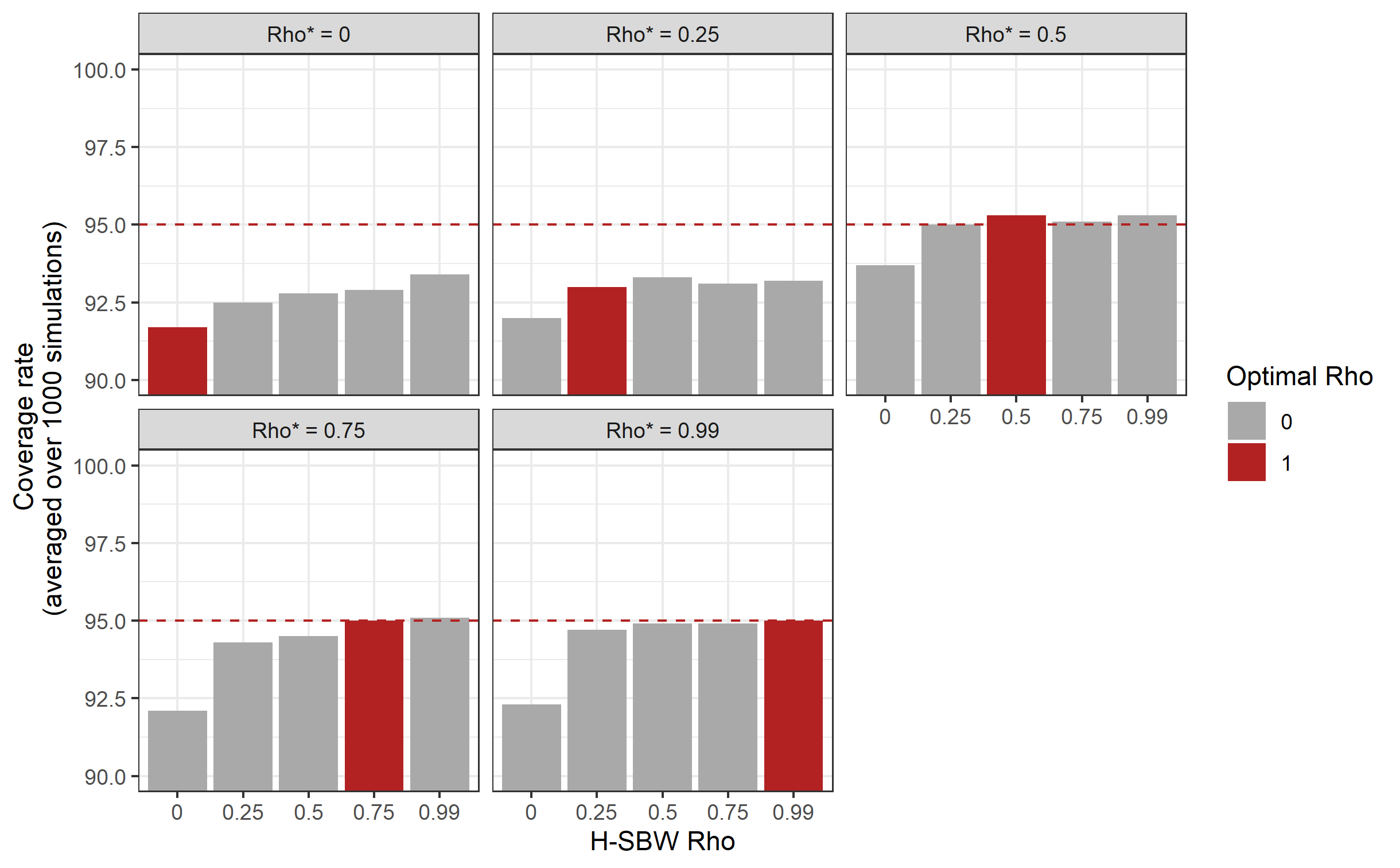
where is the estimator of with treated state removed, and . In other settings the jackknife has been shown to be a conservative approximation of the bootstrap, such as in Efron and Stein (1981), which we apply in Appendix A.1, Proposition 5 to give a partial result for our application. In a simulation study mirroring our setting with units (available in Appendix F), we obtain close to nominal coverage rates using these variance estimates.171717When more substantial undercoverage occurs it is likely due to bias.
To estimate the variance of we run an auxiliary regression model on the non-expansion states and estimate the variance of the linear combination using cluster-robust standard errors. We do not need to adjust the non-expansion state data to estimate this quantity: a linear regression line always contains the point , which are unbiased estimates of . Therefore, . Our final variance estimate is the sum of and .181818The latter is much smaller than the former – specifically, we estimate . We use the t-distribution with degrees of freedom to generate 95 percent confidence intervals.
4 Results
We first present summary statistics regarding the variability of the pre-treatment outcomes on our adjusted and unadjusted datasets. The second sub-section contains covariate balance diagnostics. The third sub-section contains a validation study, and the final sub-section contains our ETC estimates.
4.1 Covariate adjustment
Table 1 displays the sample variance of our pre-treatment outcomes among the expansion states using each covariate adjustment strategy (see Section 3.4.2 for definitions of these adjustments). Although we most heavily prioritize balancing these covariates, they are also among the least precisely estimated, as most of our other covariates average over multiple years of data. Both the homogeneous and heterogeneous adjustments reduce the variability in the data by comparable amounts. Intuitively, these adjustment reduce the likelihood that our balancing weights will fit to noise in the covariate measurements. These results are consistent across most of our other covariates. Tables containing distributional information for each covariate are available in Appendix C.
| Variable | Unadjusted | Heterogeneous | Homogeneous |
|---|---|---|---|
| Uninsured Pct 2011 | 8.35 | 8.04 | 8.05 |
| Uninsured Pct 2012 | 8.20 | 7.89 | 7.90 |
| Uninsured Pct 2013 | 8.09 | 7.78 | 7.79 |
4.2 Covariate balance
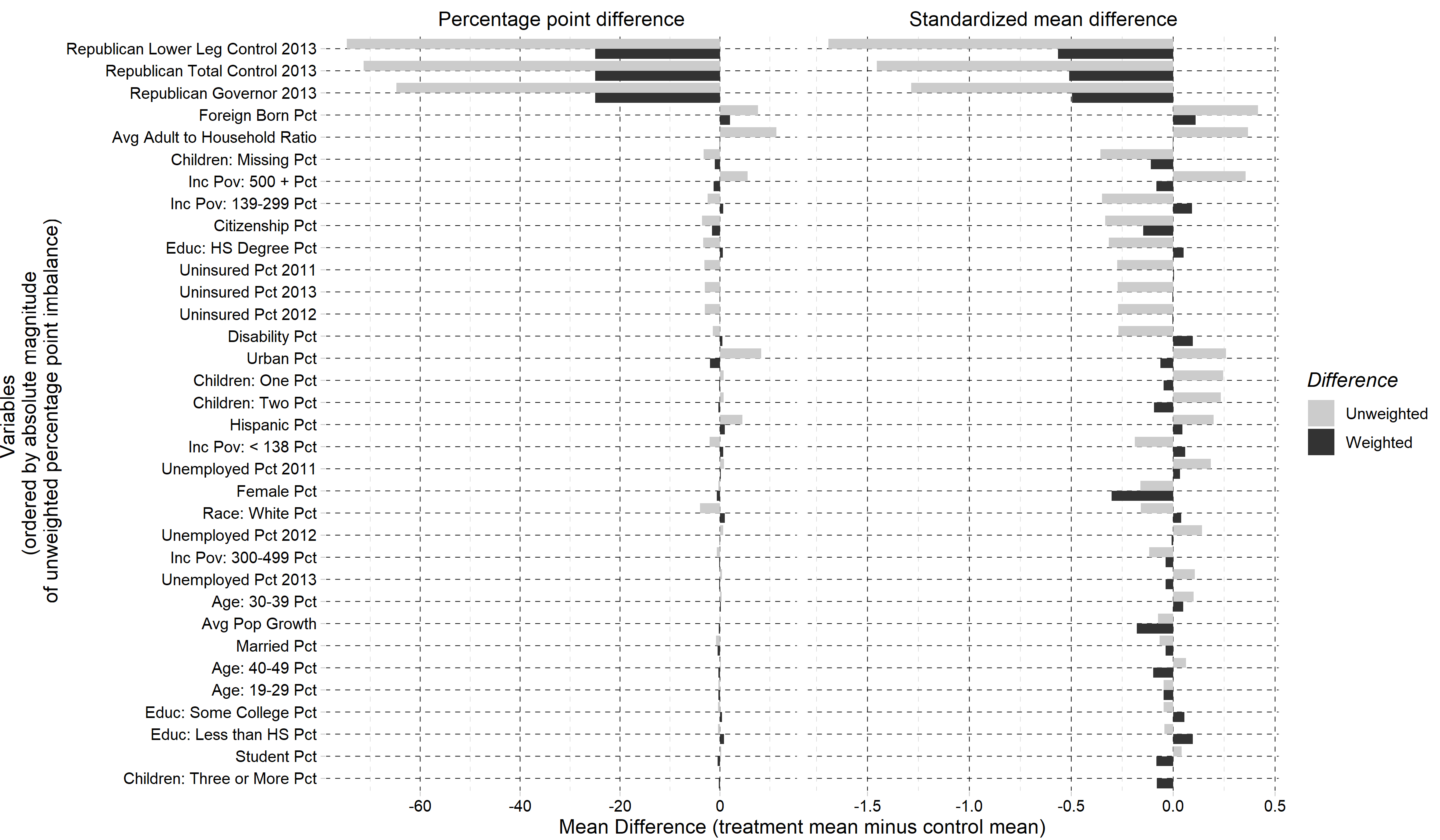
Figure 1 displays the weighted and unweighted imbalances in our adjusted covariate set (using the homogeneous adjustment) using the H-SBW weights. Our unweighted data shows substantial imbalances in the Republican governance indicators as well as pre-treatment uninsurance rates. H-SBW reduces these differences; however, some remain, particularly among the Republican governance indicators. All other imbalances are relatively small, both on the absolute difference and standardized mean difference scale. In fact, despite not targeting the SMD, all but five remaining covariate imbalances fall within 0.1 SMD, compared to 23 covariates prior to reweighting. The largest remaining imbalance on the SMD scale is among percent female (-0.3), though, as noted previously, this variable has low variance in our dataset. A complete balance table is in Appendix D.
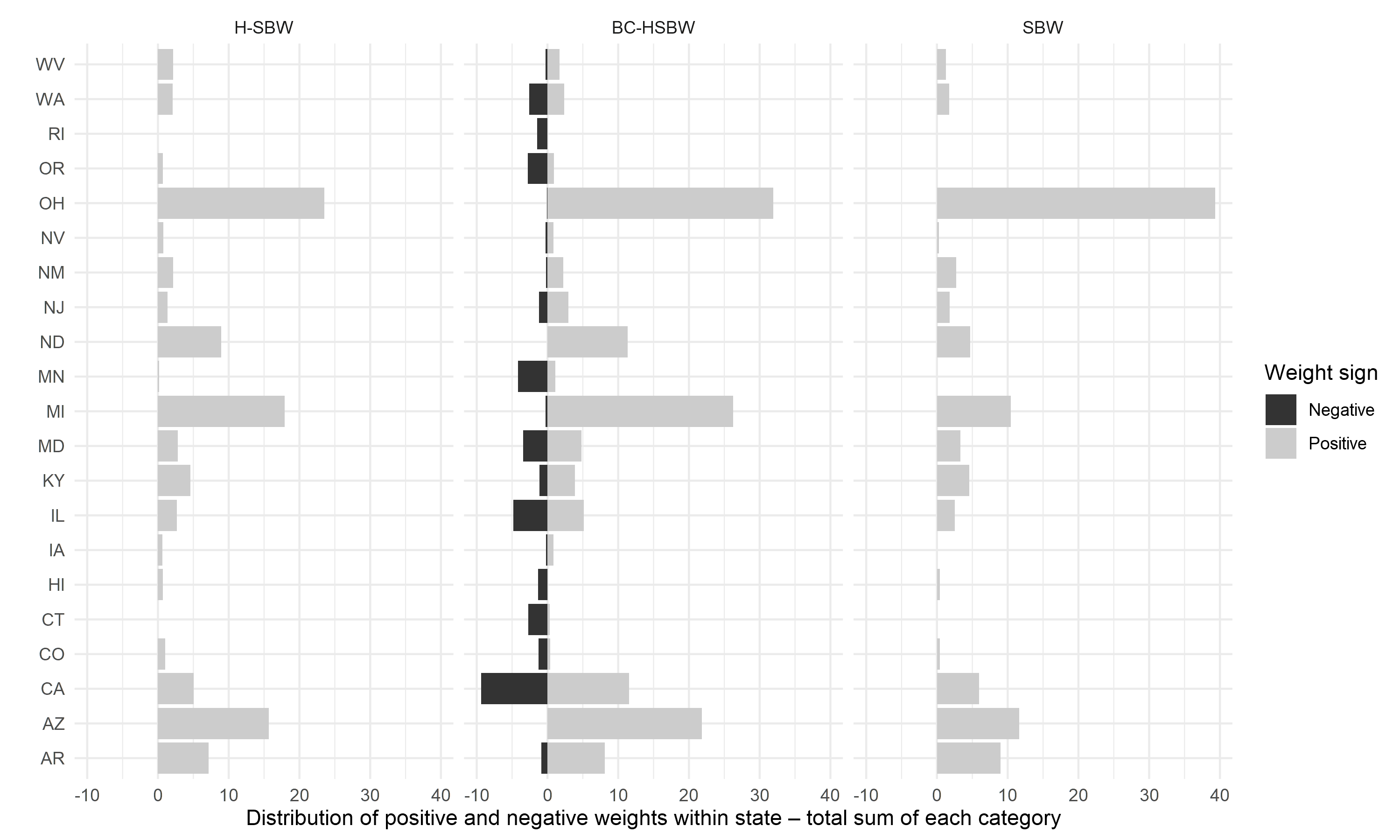
To further reduce these imbalances we augment these weights using ridge-regression. Figure 2 shows the total weights summed across states (and standardized to sum to 100) for three estimators: H-SBW, BC-HSBW, and SBW. For BC-HSBW we also display the sum of the negative weights separately from the sum of the positive weights to highlight the extrapolation. This figure illustrates two key points: first, that H-SBW more evenly disperses the weights across states relative to SBW; second, that BC-HSBW extrapolates somewhat heavily in order to achieve balance, particularly from CPUMAs in California. This is likely in part because California has the most CPUMAs of any state in the dataset.
4.3 Model validation
We compare the performance of our models by repeating the covariate adjustments and calculating our procedure on 2009-2011 ACS data to predict 2012 outcomes, and similarly for 2010-2012 data to predict 2013 outcomes for the non-expansion states. We run this procedure using the primary dataset and excluding the early expansion states. Table 2 displays the mean error and RMSE of these results, with the rows ordered by RMSE for each dataset. We see that the estimators trained on the covariate adjusted data perform substantially better than the unadjusted data and the estimators trained on the homogeneous adjustment outperform their counterparts on the heterogeneous adjustment. We therefore prioritize the results using the homogeneous adjustment. We also observe that H-SBW has comparable performance to SBW throughout.
Interestingly, the bias-corrected estimators perform relatively poorly on the primary dataset, but are the best performing estimators when excluding early expansion states – with RMSEs lower than any other estimator on the primary dataset. As the early expansion states include California, and Figure 2 shows that the bias-corrected estimators extrapolate heavily from this state, the differences in these results suggest that preventing this extrapolation may improve the model’s performance. While these results do not imply that the bias-corrected models will perform poorly when predicting in the post-treatment period on the primary dataset (or that they will perform especially well when excluding the early expansion states), it does highlight the dangers of extrapolation: linearity may approximately hold on the support of the data where we have sufficient covariate overlap, but beyond this region this may be a more costly assumption.191919In Table 13 in Appendix E, we also compare the performance against the implied regression weights from OLS and GLS. These weights exactly balance the observed covariates, but are almost always the worst performing estimators in the validation study on either dataset. This also illustrates the benefits of the regularization inherent in the bias-corrected weights.
| Primary dataset | Early expansion excluded | ||||||
|---|---|---|---|---|---|---|---|
| Sigma estimate | Estimator | Mean Error | RMSE | Sigma estimate | Estimator | Mean Error | RMSE |
| Homogeneous | SBW | -0.20 | 0.20 | Homogeneous | BC-HSBW | -0.02 | 0.07 |
| Homogeneous | H-SBW | -0.23 | 0.23 | Homogeneous | BC-SBW | -0.03 | 0.12 |
| Heterogeneous | SBW | -0.27 | 0.27 | Heterogeneous | BC-HSBW | -0.08 | 0.14 |
| Heterogeneous | H-SBW | -0.35 | 0.36 | Heterogeneous | BC-SBW | -0.07 | 0.15 |
| Homogeneous | BC-SBW | -0.39 | 0.39 | Homogeneous | H-SBW | 0.01 | 0.25 |
| Heterogeneous | BC-SBW | -0.42 | 0.42 | Homogeneous | SBW | 0.07 | 0.26 |
| Unadjusted | SBW | -0.56 | 0.56 | Heterogeneous | SBW | 0.04 | 0.28 |
| Unadjusted | H-SBW | -0.57 | 0.57 | Heterogeneous | H-SBW | -0.04 | 0.29 |
| Homogeneous | BC-HSBW | -0.58 | 0.58 | Unadjusted | SBW | -0.37 | 0.42 |
| Heterogeneous | BC-HSBW | -0.63 | 0.63 | Unadjusted | H-SBW | -0.43 | 0.46 |
| Unadjusted | BC-SBW | -0.88 | 0.88 | Unadjusted | BC-HSBW | -0.60 | 0.60 |
| Unadjusted | BC-HSBW | -0.96 | 0.96 | Unadjusted | BC-SBW | -0.70 | 0.71 |
Finally, we observe that the mean errors for the estimators generated on the unadjusted dataset are all negative, reflecting that these estimates under-predict the true uninsurance rate (see also Table 13 in Appendix E, which shows similar results for each year individually). These results likely reflect a form of regression-to-the-mean caused by overfitting our weights to noisy covariate measurements. More formally, we can think of the uninsurance rates in time period in expansion and non-expansion regions as being drawn from separate distributions with means , respectively, where . For simplicity assume that the only covariate in the outcome model at time is . Under (4), we obtain . The pre-treatment outcomes are likely positively correlated with the post-treatment outcomes, implying that . Because , when reweighting the vector of noisy pre-treatment outcomes to the expected value of the weighted measurement error should be positive. In other words, our weights are likely to favor units with covariate measurements that are greater than their true covariate values. The expected value of the weighted pre-treament outcome will then be less than the target . This implies that our estimates will be negatively biased, since .202020This phenomenon has also been discussed in the difference-in-differences and synthetic controls literature (see, e.g., Daw and Hatfield (2018)). While our covariate adjustments are meant to eliminate this bias, in practice they appear more likely only to reduce it. Assuming these errors reflect a (slight) negative bias that will also hold for our estimates of , these results suggest that the true treatment effect may be closer to zero than our estimates.
4.4 Primary Results
Table 3(a) presents all of our estimates of the ETC. Using H-SBW we estimate an effect of -2.33 (-3.54, -1.11) percentage points on our primary dataset. The SBW results are almost identical with -2.35 (-3.76, -0.95) percentage points. Compared to the unadjusted data we find very similar point estimates at -2.34 (-2.88, -1.79) percentage points for H-SBW and -2.39 (-2.99, -1.79) percentage points for SBW. We see that H-SBW reduces the confidence interval length relative to SBW on our primary dataset, though the lengths are nearly identical when excluding early expansion states. This suggests that H-SBW had at best only modest variance improvements relative to SBW in this setting. Using the adjusted covariate set also increases the length of the confidence intervals relative to the unadjusted data. This increase in the estimated variance is expected in part because the adjustment procedure generally reduces the variability in the data, as we saw in Table 1, requiring that the variance of the weights to increase to achieve approximate balance. More generally this increase also reflects the additional uncertainty due to the measurement error.
Adding the bias-correction decreases the absolute magnitude of the estimates: we estimate effects of -2.05 (-3.30, -0.80) percentage points for BC-HSBW and -2.07 (-3.14, -1.00) percentage points for BC-SBW. This contrasts to our validation study, where the bias-corrected estimators tended to predict lower uninsurance rates than the other estimators (implying we might see larger absolute magnitude effect estimates).
| Primary dataset | Early expansion excluded | ||||
|---|---|---|---|---|---|
| Weights | Adjustment | Estimate | Difference | Estimate | Difference |
| (95% CI) | (95% CI) | ||||
| H-SBW | Homogeneous | -2.33 (-3.54, -1.11) | 0.01 | -2.09 (-3.24, -0.94) | 0.19 |
| H-SBW | Unadjusted | -2.34 (-2.88, -1.79) | - | -2.28 (-2.87, -1.70) | - |
| BC-HSBW | Homogeneous | -2.05 (-3.30, -0.80) | 0.17 | -1.94 (-3.27, -0.61) | 0.28 |
| BC-HSBW | Unadjusted | -2.22 (-2.91, -1.52) | - | -2.22 (-3.14, -1.31) | - |
| SBW | Homogeneous | -2.35 (-3.76, -0.95) | 0.04 | -2.05 (-3.19, -0.91) | 0.16 |
| SBW | Unadjusted | -2.39 (-2.99, -1.79) | - | -2.21 (-2.75, -1.68) | - |
| BC-SBW | Homogeneous | -2.07 (-3.14, -1.00) | 0.13 | -1.99 (-3.33, -0.66) | 0.23 |
| BC-SBW | Unadjusted | -2.19 (-2.94, -1.45) | - | -2.23 (-3.12, -1.33) | - |
All adjusted estimators were closer to zero than the corresponding unadjusted estimators. This includes estimates using the heterogeneous adjustment (see Appendix E). However, the difference between the adjusted SBW and H-SBW and the unadjusted versions is close to zero. This contrasts with our validation study where the unadjusted SBW and H-SBW estimators ranged from about 0.3 to 0.4 percentage points lower than the adjusted estimators.212121When excluding the early expansion states, the difference between the estimates on the adjusted and unadjusted data persist but are also smaller in magnitude. We interpret this difference as due to chance: while theory and our validation study suggests that our unadjusted estimators are biased, bias only exists in expectation. Our primary dataset is a random draw where our unadjusted and adjusted estimators give similar estimates.
We next consider the sensitivity of our analysis with respect to the no anticipatory treatment effects assumption by excluding the early expansion states (California, Connecticut, Minnesota, New Jersey, and Washington) and re-running our analyses. The columns under “Early expansion excluded” in Table 3(a) reflects these results. The overall patterns of the results are consistent with our primary estimates; however, our point estimates almost all move somewhat closer to zero. This may indicate that either the primary estimates have a slight negative bias, or that these estimates have a slight positive bias. Given our analysis of the validation study we view the first case as more likely. This would imply that our primary estimators reflect a lower bound on the true treatment effect. Regardless, the differences are small relative to our uncertainty estimates. Overall we view our primary results as relatively robust to the exclusion of these states. Additional results are available in Appendix E.
5 Discussion
We divide our discussion into two sections: methodological considerations and policy considerations.
5.1 Methodological considerations and limitations
We make multiple contributions to the literature on balancing weights. First, our estimation procedure accounts for mean-zero random noise in our covariates that is uncorrelated with the outcome errors. We modify the SBW constraint set to balance on a linear approximation to the true covariate values, applying the idea of regression calibration from the measurement error literature to the context of balancing weights. Our results illustrate the benefits of this procedure: using observed pre-treatment outcomes generated by an unknown data generating mechanism, Table 2 demonstrates that our proposed estimators have better predictive performance when balancing on the adjusted covariates. This finding is consistent with concerns about overfitting to noisy covariate measurements and subsequent regression-to-the-mean.
This approach has several limitations: first, it requires access to auxiliary data with which to estimate the measurement error covariance matrix . Many applications may not have access to such information. Even without such data, could also be considered a sensitivity parameter to evaluate the robustness of results to measurement error (see, e.g., Huque, Bondell and Ryan (2014), Illenberger, Small and Shaw (2020)). Second, from a theoretic perspective, we require strong distributional assumptions on the covariates to consistently estimate using convex balancing weights. This contrasts to Gleser (1992), who shows that the OLS estimates are consistent with only very weak distributional assumptions on the data (see also Propositions 6 and 7 in Appendix A.1). This relates to a third limitation: we require strong outcome modeling assumptions. Yet by preventing extrapolation, SBW and H-SBW estimates may be less sensitive than OLS estimates to these assumptions. Our validation results support this: the standard regression calibration adjustment using OLS and GLS weights performs the worst out of any methods we consider (see Table 13 in Appendix E). In contrast, using regression-calibration with balancing weights – even when allowing for limited extrapolation using ridge-augmentation – performs better.222222We also provide a suggestion of how to adapt our procedure to accommodate a basis expansion of gaussian covariates in Appendix A.1 Remark 5 Developing methods to relax these assumptions further would be a valuable area for future work.
A final concern is that this procedure may be sub-optimal with respect to the mean-square error of our estimator. In particular, the bias induced by the measurement error decreases with the sample size used to calculate each CPUMA’s covariate values, the minimum of which were over three hundred. Yet the variance of our counterfactual estimate decreases with the number of treated states. From a theoretic perspective, the variance is of a larger order than the bias, so perhaps the bias from measurement error should not be a primary concern. Our final results support this: the changes in our results on the adjusted versus unadjusted data are of smaller magnitude than the associated uncertainty estimates. Other studies have proposed tests of whether the measurement error corrections are “worth it,” though we do not do this here (see, e.g., Gleser (1992)). However, as an informal observation, our simulation study in Appendix F shows that the MSE of the SBW estimator that naively balances on the noisy covariates is comparable to the MSE of the SBW estimator that balances on the adjusted covariates when the ratio of the variance of to the variance of is 0.95. However, even in this setting we find that confidence interval coverage can fall below nominal rates when balancing on , and that the measurement error correction can improve our ability to construct valid confidence intervals.
Our second contribution is to introduce the H-SBW objective. This objective can improve upon the SBW objective assuming that the errors in the outcome model are homoskedastic with constant positive equicorrelation within known groups of units. Assuming no measurement error and that is known, we show that H-SBW returns the minimum variance estimator within the constraint set by more evenly dispersing weights across the groups. We also demonstrate the connection between these weights and the implied weights from GLS (see Propositions 9 and 10 in Appendix A.2). While studies have considered balancing weights in settings with hierarchical data (see, e.g., Keele et al. (2020), Ben-Michael, Feller and Hartman (2021)), we are the first to our knowledge to propose changing the criterion to account for correlated outcomes.
This estimation procedure has at least three potential drawbacks. First, we make a very specific assumption on the covariance structure of the error terms that is useful for our application. For applications where a different structure is more appropriate one can still follow our approach and minimize the more general criterion . Second, we require specifying the parameters in advance. Choosing is a challenging problem shared with SBW and we do not offer any new suggestions (though see Wang and Zubizarreta (2020), who offer an interesting approach to this problem.) Choosing is a new problem of this estimation procedure. Encouragingly, our simulation study shows the H-SBW estimator for any chosen almost always has lower variance than SBW in the presence of state-level random effects (see Appendix F).232323We caution that this finding solely reflects the simulation space we examined. Even so, identifying a principled approach to choosing this parameter would be a useful future contribution. Third, in the presence of both measurement error and dependent data, using H-SBW in combination with the standard regression-calibration adjustment may be biased. This bias arises because the standard adjustment assumes independent data. Our simulations show that this bias can increase with and that SBW remains approximately unbiased if the covariates are gaussian - though even in this setting H-SBW may still yield modest MSE improvements. We also show a theoretical modification to the adjustment where H-SBW would return unbiased estimates in this setting (see Propositions 8 and 11).
5.2 Policy considerations and limitations
We estimate that had states that did not expand Medicaid in 2014 instead expanded their programs, they would have seen a -2.33 (-3.54, -1.11) percentage point change in the average adult uninsurance rate. Our validation study and robustness checks indicate that this estimate may be biased downwards (away from zero), in which case we can interpret this estimate as a lower bound on the ETC. Existing estimates place the ETT between -3 and -6 percentage points. These estimates vary depending on the targeted sub-population of interest, the data used, the level of modeling (individuals or regions), and the modeling approach (see, e.g., Courtemanche et al. (2017), Kaestner et al. (2017), Frean, Gruber and Sommers (2017)). Our estimate of the ETC are closer to zero than these estimates. When we attempt to estimate the ETT using our proposed method, the resulting estimates have high uncertainty due to limited covariate overlap.242424In particular, there were no states entirely controlled by Democrats that did not expand Medicaid. Even allowing for large imbalances, our standard error estimates were approximately three percentage points and our confidence intervals all contained zero. When estimating a simple difference-in-differences model on the unadjusted dataset we estimate that the ETT is -2.05 (-3.23, -0.87), where the standard errors account for clustering at the state level. The differences may reflect different modeling strategies and data, or it may suggest that the ETC is smaller in absolute magnitude than the ETT.
We are ultimately unable to draw any statistical conclusions about these differences; nevertheless, we continue to emphasize caution about assuming these estimands are equal. Due in part to the different covariate distributions of expansion versus non-expansion states, we may still suspect that the ETC differs from the ETT with respect to the uninsurance rates. Moreover, because almost every outcome of interest is mediated through increasing the number of insured individuals, such a difference may be important. For example, Miller, Johnson and Wherry (2021) study the effect of Medicaid expansion on mortality. Using their estimate of the ETT with respect to mortality they project that had all states expanded Medicaid, 15,600 deaths would have been avoided from 2014 through 2017. If we believe that this number increases monotonically with the number of uninsured individuals, this estimate may be an overestimate if the ETC with respect to the uninsurance rate is less than the ETT, or an underestimate if the ETC is greater than the ETT. Obtaining more precise inferences on the ETC with respect to uninsurance rates, if possible, would therefore be valuable future work.
Our analytic approach is not without limitations. Specifically, we require strong assumptions, including SUTVA, no anticipatory treatment effects, no unmeasured confounding conditional on the true covariates, and several parametric assumptions regarding the outcome and measurement error models. We address some concerns about possible violations of these assumptions. For example, our results were qualitatively similar whether we excluded possible “early expansion states,” or used different weighting strategies (including relaxing the positivity restrictions and changing the tuning parameter ). However, we do not attempt to address concerns about the impact of spillovers across regions. And while we believe that no unmeasured confounding is reasonable for this problem, we did not conduct a sensitivity analysis (see, e.g., Bonvini and Kennedy (2021)) with respect to this assumption.
Medicaid expansion remains an ongoing policy debate in the United States, where as of 2022 twelve states have not expanded their eligibility requirements. Our study estimates the effect of Medicaid expansion on adult uninsurance rates; however, the primary reason this effect interesting is that Medicaid enrollment is not automatic for eligible individuals. If the goal of Medicaid expansion is to increase insurance access for low-income adults, state policy-makers also may wish to make it easier or even automatic to enroll in Medicaid.
6 Conclusion
We predict the average change in the non-elderly adult uninsurance rate in 2014 among states that did not expand their Medicaid eligibility thresholds as if they had. We use survey data aggregated to the CPUMA-level to estimate this quantity. The resulting dataset has both measurement error in the covariates that may bias standard estimation procedures, and a hierarchical structure that may increase the variance of these same approaches. We therefore propose an estimation procedure that uses balancing weights that accounts for these problems. We demonstrate that our bias-reduction approach improves on existing methods when predicting observed outcomes from an unknown data generating mechanism. Applying this method to our problem, we estimate that states that did not expand Medicaid in 2014 would have seen a -2.33 (-3.54, -1.11) percentage point change in their adult uninsurance rates had they done so. This is the first study we are aware of that directly estimates the treatment effect on the controls with respect to Medicaid expansion. From a methodological perspective, we demonstrate the value of our proposed method relative to existing methods. From a policy-analysis perspective, we emphasize the importance of directly estimating the relevant causal quantity of interest. More generally if the goal of Medicaid expansion is to improve access to insurance, state and federal policy-makers should consider policies that make Medicaid enrollment easier if not automatic.
Acknowledgements
We gratefully acknowledge invaluable advice and comments from Zachary Branson, Riccardo Fogliato, Edward Kennedy, Brian Kovak, Akshaya Jha, Lowell Taylor, Jose Zubizaretta.
Analyses conducted using R Version 4.0.2 (R Core Team (2020)), and the optweight (Greifer (2021)) and tidyverse (Wickham et al. (2019)) packages. Programs and supporting materials are available at github.com/mrubinst757/medicaid-expansion. Proofs and additional results are available in the Appendix.
References
- Abadie, Diamond and Hainmueller (2010) {barticle}[author] \bauthor\bsnmAbadie, \bfnmAlberto\binitsA., \bauthor\bsnmDiamond, \bfnmAlexis\binitsA. and \bauthor\bsnmHainmueller, \bfnmJens\binitsJ. (\byear2010). \btitleSynthetic control methods for comparative case studies: Estimating the effect of California’s tobacco control program. \bjournalJournal of the American statistical Association \bvolume105 \bpages493–505. \endbibitem
- Abadie, Diamond and Hainmueller (2015) {barticle}[author] \bauthor\bsnmAbadie, \bfnmAlberto\binitsA., \bauthor\bsnmDiamond, \bfnmAlexis\binitsA. and \bauthor\bsnmHainmueller, \bfnmJens\binitsJ. (\byear2015). \btitleComparative politics and the synthetic control method. \bjournalAmerican Journal of Political Science \bvolume59 \bpages495–510. \endbibitem
- Ben-Michael, Feller and Hartman (2021) {barticle}[author] \bauthor\bsnmBen-Michael, \bfnmEli\binitsE., \bauthor\bsnmFeller, \bfnmAvi\binitsA. and \bauthor\bsnmHartman, \bfnmErin\binitsE. (\byear2021). \btitleMultilevel calibration weighting for survey data. \bjournalarXiv preprint arXiv:2102.09052. \endbibitem
- Ben-Michael, Feller and Rothstein (2021) {barticle}[author] \bauthor\bsnmBen-Michael, \bfnmEli\binitsE., \bauthor\bsnmFeller, \bfnmAvi\binitsA. and \bauthor\bsnmRothstein, \bfnmJesse\binitsJ. (\byear2021). \btitleThe augmented synthetic control method. \bjournalJournal of the American Statistical Association \bvolumejust-accepted \bpages1–34. \endbibitem
- Bonvini and Kennedy (2021) {barticle}[author] \bauthor\bsnmBonvini, \bfnmMatteo\binitsM. and \bauthor\bsnmKennedy, \bfnmEdward H\binitsE. H. (\byear2021). \btitleSensitivity analysis via the proportion of unmeasured confounding. \bjournalJournal of the American Statistical Association \bpages1–11. \endbibitem
- Botosaru and Ferman (2019) {barticle}[author] \bauthor\bsnmBotosaru, \bfnmIrene\binitsI. and \bauthor\bsnmFerman, \bfnmBruno\binitsB. (\byear2019). \btitleOn the role of covariates in the synthetic control method. \bjournalThe Econometrics Journal \bvolume22 \bpages117–130. \endbibitem
- Buonaccorsi (2010) {bbook}[author] \bauthor\bsnmBuonaccorsi, \bfnmJohn P\binitsJ. P. (\byear2010). \btitleMeasurement error: models, methods, and applications. \bpublisherChapman and Hall/CRC. \endbibitem
- Cameron, Gelbach and Miller (2008) {barticle}[author] \bauthor\bsnmCameron, \bfnmA Colin\binitsA. C., \bauthor\bsnmGelbach, \bfnmJonah B\binitsJ. B. and \bauthor\bsnmMiller, \bfnmDouglas L\binitsD. L. (\byear2008). \btitleBootstrap-based improvements for inference with clustered errors. \bjournalThe Review of Economics and Statistics \bvolume90 \bpages414–427. \endbibitem
- Cameron and Miller (2015) {barticle}[author] \bauthor\bsnmCameron, \bfnmA Colin\binitsA. C. and \bauthor\bsnmMiller, \bfnmDouglas L\binitsD. L. (\byear2015). \btitleA practitioner’s guide to cluster-robust inference. \bjournalJournal of human resources \bvolume50 \bpages317–372. \endbibitem
- Carroll et al. (2006) {bbook}[author] \bauthor\bsnmCarroll, \bfnmRaymond J\binitsR. J., \bauthor\bsnmRuppert, \bfnmDavid\binitsD., \bauthor\bsnmStefanski, \bfnmLeonard A\binitsL. A. and \bauthor\bsnmCrainiceanu, \bfnmCiprian M\binitsC. M. (\byear2006). \btitleMeasurement error in nonlinear models: a modern perspective. \bpublisherCRC press. \endbibitem
- Chattopadhyay and Zubizarreta (2021) {barticle}[author] \bauthor\bsnmChattopadhyay, \bfnmAmbarish\binitsA. and \bauthor\bsnmZubizarreta, \bfnmJose R\binitsJ. R. (\byear2021). \btitleOn the implied weights of linear regression for causal inference. \bjournalarXiv preprint arXiv:2104.06581. \endbibitem
- Courtemanche et al. (2017) {barticle}[author] \bauthor\bsnmCourtemanche, \bfnmCharles\binitsC., \bauthor\bsnmMarton, \bfnmJames\binitsJ., \bauthor\bsnmUkert, \bfnmBenjamin\binitsB., \bauthor\bsnmYelowitz, \bfnmAaron\binitsA. and \bauthor\bsnmZapata, \bfnmDaniela\binitsD. (\byear2017). \btitleEarly impacts of the Affordable Care Act on health insurance coverage in Medicaid expansion and non-expansion states. \bjournalJournal of Policy Analysis and Management \bvolume36 \bpages178–210. \endbibitem
- Daw and Hatfield (2018) {barticle}[author] \bauthor\bsnmDaw, \bfnmJamie R\binitsJ. R. and \bauthor\bsnmHatfield, \bfnmLaura A\binitsL. A. (\byear2018). \btitleMatching and Regression to the Mean in Difference-in-Differences Analysis. \bjournalHealth services research \bvolume53 \bpages4138–4156. \endbibitem
- Deville and Särndal (1992) {barticle}[author] \bauthor\bsnmDeville, \bfnmJean-Claude\binitsJ.-C. and \bauthor\bsnmSärndal, \bfnmCarl-Erik\binitsC.-E. (\byear1992). \btitleCalibration estimators in survey sampling. \bjournalJournal of the American statistical Association \bvolume87 \bpages376–382. \endbibitem
- Deville, Särndal and Sautory (1993) {barticle}[author] \bauthor\bsnmDeville, \bfnmJean-Claude\binitsJ.-C., \bauthor\bsnmSärndal, \bfnmCarl-Erik\binitsC.-E. and \bauthor\bsnmSautory, \bfnmOlivier\binitsO. (\byear1993). \btitleGeneralized raking procedures in survey sampling. \bjournalJournal of the American statistical Association \bvolume88 \bpages1013–1020. \endbibitem
- D’Amour et al. (2021) {barticle}[author] \bauthor\bsnmD’Amour, \bfnmAlexander\binitsA., \bauthor\bsnmDing, \bfnmPeng\binitsP., \bauthor\bsnmFeller, \bfnmAvi\binitsA., \bauthor\bsnmLei, \bfnmLihua\binitsL. and \bauthor\bsnmSekhon, \bfnmJasjeet\binitsJ. (\byear2021). \btitleOverlap in observational studies with high-dimensional covariates. \bjournalJournal of Econometrics \bvolume221 \bpages644–654. \endbibitem
- Efron and Stein (1981) {barticle}[author] \bauthor\bsnmEfron, \bfnmBradley\binitsB. and \bauthor\bsnmStein, \bfnmCharles\binitsC. (\byear1981). \btitleThe jackknife estimate of variance. \bjournalThe Annals of Statistics \bpages586–596. \endbibitem
- Frean, Gruber and Sommers (2017) {barticle}[author] \bauthor\bsnmFrean, \bfnmMolly\binitsM., \bauthor\bsnmGruber, \bfnmJonathan\binitsJ. and \bauthor\bsnmSommers, \bfnmBenjamin D\binitsB. D. (\byear2017). \btitlePremium subsidies, the mandate, and Medicaid expansion: Coverage effects of the Affordable Care Act. \bjournalJournal of Health Economics \bvolume53 \bpages72–86. \endbibitem
- Gleser (1992) {barticle}[author] \bauthor\bsnmGleser, \bfnmLeon Jay\binitsL. J. (\byear1992). \btitleThe importance of assessing measurement reliability in multivariate regression. \bjournalJournal of the American Statistical Association \bvolume87 \bpages696–707. \endbibitem
- Greifer (2021) {bmanual}[author] \bauthor\bsnmGreifer, \bfnmNoah\binitsN. (\byear2021). \btitleoptweight: Targeted Stable Balancing Weights Using Optimization \bnoteR package version 0.2.5.9000. \endbibitem
- Haberman (1984) {barticle}[author] \bauthor\bsnmHaberman, \bfnmShelby J\binitsS. J. (\byear1984). \btitleAdjustment by minimum discriminant information. \bjournalThe Annals of Statistics \bpages971–988. \endbibitem
- Hainmueller (2012) {barticle}[author] \bauthor\bsnmHainmueller, \bfnmJens\binitsJ. (\byear2012). \btitleEntropy balancing for causal effects: A multivariate reweighting method to produce balanced samples in observational studies. \bjournalPolitical analysis \bvolume20 \bpages25–46. \endbibitem
- Huque, Bondell and Ryan (2014) {barticle}[author] \bauthor\bsnmHuque, \bfnmMd Hamidul\binitsM. H., \bauthor\bsnmBondell, \bfnmHoward D\binitsH. D. and \bauthor\bsnmRyan, \bfnmLouise\binitsL. (\byear2014). \btitleOn the impact of covariate measurement error on spatial regression modelling. \bjournalEnvironmetrics \bvolume25 \bpages560–570. \endbibitem
- Illenberger, Small and Shaw (2020) {barticle}[author] \bauthor\bsnmIllenberger, \bfnmNicholas A\binitsN. A., \bauthor\bsnmSmall, \bfnmDylan S\binitsD. S. and \bauthor\bsnmShaw, \bfnmPamela A\binitsP. A. (\byear2020). \btitleImpact of Regression to the Mean on the Synthetic Control Method: Bias and Sensitivity Analysis. \bjournalEpidemiology \bvolume31 \bpages815–822. \endbibitem
- Imai and Ratkovic (2014) {barticle}[author] \bauthor\bsnmImai, \bfnmKosuke\binitsK. and \bauthor\bsnmRatkovic, \bfnmMarc\binitsM. (\byear2014). \btitleCovariate balancing propensity score. \bjournalJournal of the Royal Statistical Society: Series B: Statistical Methodology \bpages243–263. \endbibitem
- Imbens (2004) {barticle}[author] \bauthor\bsnmImbens, \bfnmGuido W\binitsG. W. (\byear2004). \btitleNonparametric estimation of average treatment effects under exogeneity: A review. \bjournalReview of Economics and statistics \bvolume86 \bpages4–29. \endbibitem
- Kaestner et al. (2017) {barticle}[author] \bauthor\bsnmKaestner, \bfnmRobert\binitsR., \bauthor\bsnmGarrett, \bfnmBowen\binitsB., \bauthor\bsnmChen, \bfnmJiajia\binitsJ., \bauthor\bsnmGangopadhyaya, \bfnmAnuj\binitsA. and \bauthor\bsnmFleming, \bfnmCaitlyn\binitsC. (\byear2017). \btitleEffects of ACA Medicaid expansions on health insurance coverage and labor supply. \bjournalJournal of Policy Analysis and Management \bvolume36 \bpages608–642. \endbibitem
- Keele et al. (2020) {barticle}[author] \bauthor\bsnmKeele, \bfnmLuke\binitsL., \bauthor\bsnmBen-Michael, \bfnmEli\binitsE., \bauthor\bsnmFeller, \bfnmAvi\binitsA., \bauthor\bsnmKelz, \bfnmRachel\binitsR. and \bauthor\bsnmMiratrix, \bfnmLuke\binitsL. (\byear2020). \btitleHospital Quality Risk Standardization via Approximate Balancing Weights. \bjournalarXiv preprint arXiv:2007.09056. \endbibitem
- Kline (2011) {barticle}[author] \bauthor\bsnmKline, \bfnmPatrick\binitsP. (\byear2011). \btitleOaxaca-Blinder as a reweighting estimator. \bjournalAmerican Economic Review \bvolume101 \bpages532–37. \endbibitem
- Ladhania et al. (2021) {barticle}[author] \bauthor\bsnmLadhania, \bfnmRahul\binitsR., \bauthor\bsnmHaviland, \bfnmAmelia M\binitsA. M., \bauthor\bsnmVenkat, \bfnmArvind\binitsA., \bauthor\bsnmTelang, \bfnmRahul\binitsR. and \bauthor\bsnmPines, \bfnmJesse M\binitsJ. M. (\byear2021). \btitleThe effect of Medicaid expansion on the nature of new enrollees’ emergency department use. \bjournalMedical Care Research and Review \bvolume78 \bpages24–35. \endbibitem
- Miller, Johnson and Wherry (2021) {barticle}[author] \bauthor\bsnmMiller, \bfnmSarah\binitsS., \bauthor\bsnmJohnson, \bfnmNorman\binitsN. and \bauthor\bsnmWherry, \bfnmLaura R\binitsL. R. (\byear2021). \btitleMedicaid and mortality: new evidence from linked survey and administrative data. \bjournalThe Quarterly Journal of Economics \bvolume136 \bpages1783–1829. \endbibitem
- Rubin (2005) {barticle}[author] \bauthor\bsnmRubin, \bfnmDonald B\binitsD. B. (\byear2005). \btitleCausal inference using potential outcomes: Design, modeling, decisions. \bjournalJournal of the American Statistical Association \bvolume100 \bpages322–331. \endbibitem
- Särndal and Lundström (2005) {bbook}[author] \bauthor\bsnmSärndal, \bfnmCarl-Erik\binitsC.-E. and \bauthor\bsnmLundström, \bfnmSixten\binitsS. (\byear2005). \btitleEstimation in surveys with nonresponse. \bpublisherJohn Wiley & Sons. \endbibitem
- Sommers et al. (2012) {barticle}[author] \bauthor\bsnmSommers, \bfnmBen\binitsB., \bauthor\bsnmKronick, \bfnmRick\binitsR., \bauthor\bsnmFinegold, \bfnmKenneth\binitsK., \bauthor\bsnmPo, \bfnmRosa\binitsR., \bauthor\bsnmSchwartz, \bfnmKaryn\binitsK. and \bauthor\bsnmGlied, \bfnmSherry\binitsS. (\byear2012). \btitleUnderstanding participation rates in Medicaid: implications for the Affordable Care Act. \bjournalPublic Health \bvolume93 \bpages67–74. \endbibitem
- R Core Team (2020) {bmanual}[author] \bauthor\bsnmR Core Team (\byear2020). \btitleR: A Language and Environment for Statistical Computing \bpublisherR Foundation for Statistical Computing, \baddressVienna, Austria. \endbibitem
- Wang and Zubizarreta (2020) {barticle}[author] \bauthor\bsnmWang, \bfnmYixin\binitsY. and \bauthor\bsnmZubizarreta, \bfnmJose R\binitsJ. R. (\byear2020). \btitleMinimal dispersion approximately balancing weights: asymptotic properties and practical considerations. \bjournalBiometrika \bvolume107 \bpages93–105. \endbibitem
- Wickham et al. (2019) {barticle}[author] \bauthor\bsnmWickham, \bfnmHadley\binitsH., \bauthor\bsnmAverick, \bfnmMara\binitsM., \bauthor\bsnmBryan, \bfnmJennifer\binitsJ., \bauthor\bsnmChang, \bfnmWinston\binitsW., \bauthor\bsnmMcGowan, \bfnmLucy D’Agostino\binitsL. D., \bauthor\bsnmFrançois, \bfnmRomain\binitsR., \bauthor\bsnmGrolemund, \bfnmGarrett\binitsG., \bauthor\bsnmHayes, \bfnmAlex\binitsA., \bauthor\bsnmHenry, \bfnmLionel\binitsL., \bauthor\bsnmHester, \bfnmJim\binitsJ., \bauthor\bsnmKuhn, \bfnmMax\binitsM., \bauthor\bsnmPedersen, \bfnmThomas Lin\binitsT. L., \bauthor\bsnmMiller, \bfnmEvan\binitsE., \bauthor\bsnmBache, \bfnmStephan Milton\binitsS. M., \bauthor\bsnmMüller, \bfnmKirill\binitsK., \bauthor\bsnmOoms, \bfnmJeroen\binitsJ., \bauthor\bsnmRobinson, \bfnmDavid\binitsD., \bauthor\bsnmSeidel, \bfnmDana Paige\binitsD. P., \bauthor\bsnmSpinu, \bfnmVitalie\binitsV., \bauthor\bsnmTakahashi, \bfnmKohske\binitsK., \bauthor\bsnmVaughan, \bfnmDavis\binitsD., \bauthor\bsnmWilke, \bfnmClaus\binitsC., \bauthor\bsnmWoo, \bfnmKara\binitsK. and \bauthor\bsnmYutani, \bfnmHiroaki\binitsH. (\byear2019). \btitleWelcome to the tidyverse. \bjournalJournal of Open Source Software \bvolume4 \bpages1686. \bdoi10.21105/joss.01686 \endbibitem
- Zhang et al. (2019) {barticle}[author] \bauthor\bsnmZhang, \bfnmZhongheng\binitsZ., \bauthor\bsnmKim, \bfnmHwa Jung\binitsH. J., \bauthor\bsnmLonjon, \bfnmGuillaume\binitsG., \bauthor\bsnmZhu, \bfnmYibing\binitsY. \betalet al. (\byear2019). \btitleBalance diagnostics after propensity score matching. \bjournalAnnals of translational medicine \bvolume7. \endbibitem
- Zubizarreta (2015) {barticle}[author] \bauthor\bsnmZubizarreta, \bfnmJosé R\binitsJ. R. (\byear2015). \btitleStable weights that balance covariates for estimation with incomplete outcome data. \bjournalJournal of the American Statistical Association \bvolume110 \bpages910–922. \endbibitem
Appendix A Proofs
We divide our proofs into three sections: the first two consist of propositions and the third contains the proofs of the propositions. In the first section our propositions pertain to the performance of SBW under the classical measurement error model. Our key results are that the bias of the SBW estimator is equivalent to the bias of the OLS estimator and that regression-calibration techniques can be used in this setting to obtain consistent estimators. However, these results assume that the data are gaussian. We also show that if the data are not gaussian, the OLS estimator using regression-calibration remains consistent, while the SBW estimator may be biased; however, this can be corrected if other distributional assumptions are made in place of gaussianity. In our second section we consider the properties of the H-SBW objective when the true covariates are observed. We show that if our assumed covariance structure for the outcome errors is correct, H-SBW produces the minimum conditional-on-X variance estimator within the constraint set. We also show how a generalized form of H-SBW weights relate to the implied regression weights from Generalized Least Squares (GLS). We conclude by showing that H-SBW may yield biased estimates if we do not correctly model the dependence structure of the data. Section A.3 contains all of the proofs.
A.1 SBW and classical measurement error
We begin by showing several results regarding the bias of the OLS and SBW estimators under the classical errors-in-variables model. First, we show that without adjustment for errors-in-covariates, the bias of the SBW estimator that sets (i.e. reweights the treated units to exactly balance the control units) is equal to the bias of the OLS estimator. Second, we show that if the observed covariate values for the treated data can be replaced by their conditional expectations given the noisy observations, then the SBW estimator will be unbiased and consistent. Third, we consider the case where must be estimated, and show that the SBW estimator is consistent if we replace by a consistent estimate . Finally, we remove the assumption that is gaussian, and show that while the OLS estimator remains unbiased under weaker assumptions, the SBW estimator does not, and we show a general expression for the asymptotic bias. We take the perspective throughout that is random among the treated units but fixed for the control units.
We assume that equations (3) - (7) hold. For simplicity, we additionally assume that
| (18) |
noting that implies . These assumptions imply that the data from the treated units are i.i.d., though for consistency of notation we continue to index the data by and and assume that the state-membership for each CPUMA is known. The covariate observations of the treated units can then be seen to have covariance matrix
and the conditional expectation of given for the treated units can be seen to equal
where
To ease notation, we abbreviate and similarly .
In Propositions 6, 7, and part of Proposition 1, we will remove the Gaussian covariate assumption given by (7). In its place, we will instead consider the weaker assumption that the empirical covariance of has a limit ,
| (19) |
which implies a similar limit for the noisy observations ,
| (20) |
where we have used the independence of the noise terms , and similarly that
| (21) |
where we have additionally used the linear model for given by (4).
We first consider estimation without adjustment for errors in covariates. Proposition 1 states that the unadjusted OLS and SBW estimators have equal bias, with the bias of the OLS estimator remaining unchanged if the gaussian assumption of (6) is removed.
Proposition 1.
Let (3) - (7) and (18) hold. Let denote the unadjusted OLS estimator of ,
| (22) |
which induces the OLS estimator of given by
Let denote the unadjusted SBW weights under exact balance, found by solving (11) with constraint set , which induces the SBW estimator of given by
Then the estimators and have equal bias, satisfying
To study the SBW estimator with covariate adjustment, we first consider an idealized version where and are known, so that is also known. Proposition 2 shows that the resulting estimate of is unbiased if .
Proposition 2.
let be the solution to the SBW objective defined over the constraint set , and let be the SBW estimator . This estimator is unbiased for .
Proposition 3 shows that the variance of this idealized SBW estimator goes to zero, implying consistency.
Proposition 3.
Let (3) - (7) and (18) hold, and let and be defined as in Proposition 2. Then the conditional variance of the estimation error is given by
with and both behaving as as .
In practice, the idealized SBW estimator considered in Propositions 2 and 3 cannot be used, as and are not known, but instead must be estimated from auxiliary data. Proposition 4 states that if these estimates are consistent, then the resulting adjusted SBW estimator for is also consistent if .
Proposition 4.
In (17) we propose a leave-one-state-out jackknife estimate of variance. Following Efron and Stein (1981), this estimate can be decomposed a conservatively biased estimate of the variance of given a sample size of treated states, plus a heuristic adjustment to go from sample size to sample size , when treating the observations of the control states as fixed.
Proposition 5.
Let (3) - (7) hold, and additionally assume that , the number of CPUMAs, is i.i.d. in the treated states. Let , where
| (23) |
with and as defined for (17). Then is conservatively biased for the variance of the leave-one-state-out estimate,
where can be seen to equal the estimator under a sample size of treated states.
As the gaussian covariate assumption given by (7) is strong, it would be desirable if the adjusted OLS or SBW estimators were consistent even for non-gaussian . Proposition 6 shows under mild assumptions that this is in fact true when running OLS on the adjusted covariates.
Proposition 6.
Let (3) - (6), and (18)- (19) hold, with invertible. Let denote the adjusted OLS estimates of , solving
where with . Then the adjusted OLS estimator of given by
remains consistent if the gaussian assumption given by (6) is removed.
However, the same does not hold for the adjusted SBW estimator. Proposition 7 gives an expression for its bias when the covariates are non-gaussian.
Proposition 7.
Let the assumptions of Proposition 6 hold. Let solve the SBW objective over the constraint set where and are defined as in Proposition 6. Let denote the set of indices where is non-zero,
with cardinality , and let and denote the empirical mean and covariance of ,
with the analogous empirical mean of and the empirical cross covariance,
Then if the gaussian assumption given by (6) is removed, the adjusted SBW estimator for given by
may be biased for , with estimation error given by
| (24) |
which need not converge to zero unless , , and .
Proposition 8 shows that if the conditional expectations can be computed for the treated units (which may be computationally difficult or require strong modeling assumptions if the data is non-gaussian, or if dependencies exist between CPUMAs), then SBW yields unbiased estimates.
Proposition 8.
remark 1.
While we have assumed that for simplicity in our propositions, removing this assumption simply leads to the additional term in the error of the SBW estimator of . This again has expectation zero, because the weights remain independent of the error in the outcomes. Allowing non-zero also adds a term to the estimator variance (conditional on ) equal to , which does not change the variance bound given by Proposition 3.
remark 2.
For the adjusted OLS estimator, in which is estimated using the adjusted covariates , in practice we must estimate with some estimator that relies on an estimate . As long as is consistent for then the OLS estimator will also be consistent by the continuous mapping theorem.
remark 3.
As Proposition 5 implies that is conservatively biased only up the heuristic scaling term, it may be preferable to remove this scaling term entirely, inflating the variance estimate slightly. While the proposition considers the marginal variance of the estimator , a confidence interval using the conditional variance (see, e.g., Buonaccorsi (2010), who discuss using a modification of the parametric bootstrap for parameters estimated via OLS in this setting) may be of interest, potentially leading to smaller intervals and more precise inference.
remark 4.
To see how Proposition 7 implies that the adjusted SBW estimate may be biased in non-gaussian settings, we observe that as the set in Proposition 7 will depend on the values of the covariates and observation noise , the values of and may differ systematically from their population, so that , and may not converge to their desired counterparts. While the expression for the estimation error given by (24) is asymptotic, an exact formula is given in (54) which is very similar; the only asymptotic approximations are the convergence of to and to .
remark 5.
We describe a possible direction for future work that utilizes Proposition 8. Suppose that in place of equations (5)-(7), we instead assume that is a transformation of the covariate, so that for some transformation , and that the untransformed is observed with additive noise, so that . For example, to make the linear model (4) more credible, might denote a basis expansion applied to the survey sampled covariates for each unit. If, analogous to assumptions (6) and (7), the original covariates and measurement error can be assumed to be i.i.d. gaussian, so that the treated units satisfy
then the posterior distribution of given for the treated units will also be gaussian
where and are given for the treated units by
with analogous expressions for the control units. This suggests that if auxiliary data can be used to find , , and as before, then could be estimated by using monte carlo methods. Specifically, for each unit we can generate random variates that are i.i.d. normal with mean and covariance , and estimate by the average of . To estimate the SBW constraint set , then could be estimated by averaging . By Proposition 8 the resulting SBW weights would yield unbiased estimates.
A.2 Properties of H-SBW
Here we consider an H-SBW setting where so that the true covariates are observed. By (4), the outcomes have CPUMA level noise terms , and also state-level noise terms that correlate the outcomes of CPUMAs in the same state. Proposition 9 states that if is the within-state correlation of these error terms, the H-SBW estimator produces the minimum conditional-on-X variance estimator of within the constraint set.
Proposition 9.
Consider the outcome model in (4). Assume the errors are homoskedastic and have finite variance and , and let be the within-state correlation of the error terms. Let be the weights that solve (14) for known parameter across the constraint set for any . Then the H-SBW estimator of ,
is the minimum conditional-on-X variance estimator of within the constraint set .
The SBW and H-SBW objective functions take the generic form : SBW takes , while H-SBW specifies an that allows for homoskedastic errors with positive within-state equicorrelation. Analogous versions hence exist for any assumed covariance structure . Proposition 10 highlights connections between this generic form and GLS, showing that when exact balance is possible we can express the generic form of the problem as the implied regression weights from GLS estimated on a subset of the data. Similar results connecting balancing weights to regression weights can be found throughout the literature. For example, see Kline (2011), Ben-Michael, Feller and Rothstein (2021), Chattopadhyay and Zubizarreta (2021), who connect balancing weights to regression weights for OLS, ridge-regression, and weighted least-squares and two-stage-least-squares; our result adds by connecting balancing weights to regression weights for GLS.
Proposition 10.
Let solve the optimization problem
| (25) |
with positive definite. Let denote the indices of its non-zero entries. Then also solves the problem
| (26) |
and hence has non-zero entries satisfying
| (27) |
where is the matrix whose columns are , is the submatrix of whose rows and columns are in , is the column vector of ones, and is the vector . These weights are equivalent to the implied regression weights when running GLS on the subset .
remark 6.
To lighten notation, we have used (a vector subtracted from a matrix) to mean , so that each column of is centered by .
remark 7.
Removing the positivity constraint from the generic form of the SBW objective implies that the resulting weights are equivalent to the implied regression weights from GLS. This follows by noting that removing the positivity constraint from the SBW objective removes the solution’s dependence on the set . This result is a natural generalization of the connections between the implied regression weights of OLS and SBW also noted by, for example, Chattopadhyay and Zubizarreta (2021).
Proposition 11 simply states that the conclusion of Proposition 8 holds not only for SBW, but for H-SBW as well.
Proposition 11.
remark 8.
In Proposition 9, we assumed the outcomes followed (4) and the constraints balanced the means of the covariates; however, we can allow for any outcome model and our balance constraints can include any function of the covariate distribution and this result still holds conditional on (though of course the estimator may be badly biased). The key assumption is that the variability in the estimates comes from the outcome model errors, which are assumed to be homoskedastic and equicorrelated within state for known parameter .
remark 9.
Assuming that are gaussian but dependent, Proposition 11 implies that if we correctly model the correlations between the CPUMAs within states in our regression calibration step, we can use GLS or H-SBW without inducing asymptotic bias (assuming all of our models are correct). This is similar to the approach followed in Huque, Bondell and Ryan (2014), who consider parameter estimation using GLS in the context of a one-dimensional spatially-correlated covariate measured with error. We also outline in Appendix B a potential adjustment when we assume the units have a covariance structure similar to our assumptions for the outcome model errors. We evaluate this adjustment in simulations in Appendix F.
To be clear if we do not model this dependence structure we cannot generally use the simple adjustment provided in (8) in combination with GLS to obtain asymptotically unbiased estimates. Intuitively this is because the implied weights from GLS depend on the dependence between CPUMAs within states, which (8) does not correctly account for. By contrast, Proposition 6 shows that we safely can ignore such dependence when using regression-calibration with OLS (as long as a probability limit exists for the empirical covariance matrix).
remark 10.
In our simulation study in Appendix F we obtain an approximately unbiased estimate when using SBW using the simple adjustment provided in (8) with dependent gaussian data. We conjecture that the set may have some limiting boundary. If true, the characterization of SBW weights as regression weights in Proposition 10 would imply that the SBW weight is fixed conditional on the input data point asymptotically. The error of the estimator could then decompose as a function of , which is independent of given . This implies that it would suffice to balance on .
A.3 Proofs
We begin by establishing the following identity for our target parameter defined in (1).
| (28) |
where and .
Proof of (28).
Using our causal and modeling assumptions we have that:
where the first equality follows from unconfoundedness, the second equality from consistency, the third from our parametric modeling assumptions, and the fourth by definition of . The final equation follows from averaging over the control units. ∎
Proof of Propositon 1.
It can be seen from (8) that for all ,
where may be viewed as an independent zero-mean noise term. Plugging into (4) yields
| (29) |
To show that and have identical bias, we compute their expectations:
| (32) | ||||
| (33) | ||||
| (34) | ||||
| (35) | ||||
| (36) | ||||
| (37) | ||||
| (38) |
where (32) holds by the assumed linear model for given by (4); (33) and (38) hold because the SBW algorithm enforces that , which has expectation , and because is zero-mean and independent of and hence independent of ; (34) holds by definition of and the assumed linear model in (4); (35) is the tower property of expectations; (36) follows because and are deterministic given ; and (37) uses the expression for the conditional expectation given by (8). It can be seen that (31) and (38) are equal, and hence show that and have equal bias.
It remains to show that the bias of the OLS estimator is unchanged if the gaussian assumption is relaxed so that (8) no longer holds. It follows from (22) that is asymptotically given by
from which the result follows by the same steps used to show (31).
∎
Proof of Proposition 3.
To derive , we use
| (42) | ||||
| (43) | ||||
| (44) | ||||
| (45) |
where (42) follows from (41), (43) holds because the tuples are i.i.d, and (44) holds because is fixed given and are jointly normal.
To upper bound the conditional variance given by (45), we will construct a feasible solution to the SBW objective over the constraint set such that . As the optimal solution satisfies , the result follows.
Our construction is the following. Divide the treated units into subsets of size , and a remainder subset. For the subsets , let denote its covariates, the conditional expectation , and the solution to the SBW objective over the constraint set , with if the constraint set is infeasible. As the units are assumed to be i.i.d., it follows that are also i.i.d. Let be large enough so that each has positive probability of being non-zero.
Let denote the number of subsets whose is non-zero. As each non-zero weight vector is feasible for , it can be seen that the concatenated vector is feasible for . As the weights are i.i.d, it follows that which equals converges in probability to , proving the bound on .
To show this rate also holds for , we can apply the law of total variance to ,
observing that by Proposition 2, so that (ii) is zero. To show that term (i) is , we observe that as and is bounded (since is non-negative and sums to 1), it follows that must be as well. ∎
Proof of Proposition 4.
Following Proposition 2, assuming we can decompose the error of the estimator as follows:
| (46) | ||||
| (47) | ||||
| (48) |
We observe that term (i) goes to zero by the law of large numbers. Term (iii) goes to zero because (since and sums to 1), and because converges to uniformly over all units as and converge.
To show that (ii) goes to zero, we will show that conditioned on , (ii) is zero mean and has variance going to zero. Conditioned on , is fixed; this implies that conditioned on , term (ii) is zero-mean, and has conditional variance
By a construction argument identical to one used in the proof of Proposition 3, it can be shown that , implying that the conditional variance goes to zero as well. ∎
Proof of Proposition 5.
Let denote the observed outcomes and covariates corresponding to the CPUMAs in state . Under our assumptions, it holds that is i.i.d. for the treated states. It can also be seen that is a symmetric function of the treated state observations . It follows that equation (1.6) of Efron and Stein (1981) can be seen to apply to our setting; as this equation is equal to (23), this proves the result. ∎
Proof of Proposition 6.
Proof of Proposition 7.
We will use Proposition 10 which is proved later in this section. To apply it, we let , , and . Using , we find that
| (50) |
and hence that . Plugging into (27) yields
| (51) |
As for the treated units, the SBW estimator of can be seen to equal
| (52) | ||||
| (53) | ||||
| (54) | ||||
| (55) | ||||
where (52) uses the expression for given by (51; (53) follows by algebraic manipulations, and notes that ; (54) adds and subtracts , substitutes for using (50), and groups the terms into (i), (ii), and (iii); and (55) substitutes for and uses and .
It can be seen that terms (i), (ii), and (iii) each go to zero if , , and , proving the result. ∎
Proof of Propositions 8 and 11.
We prove the result for H-SBW only, as letting includes SBW as a special case. Following the derivation of (41) with the H-SBW weights in place of , it can be shown that:
Conditional on (and assuming that the correspondence between states and CPUMAs is known), is fixed and equals which has mean zero, proving the result. ∎
Proof of Proposition 9.
where the second line follows by dividing by . By definition of the H-SBW objective, which minimizes this function for known , the H-SBW estimator must produce the minimum conditional-on-X variance estimator within the constraint set. ∎
Proof of Proposition 10.
To show that solves (26), we first observe that it is a feasible solution, by definition of . The result can then be proven by contradiction: if is feasible but does not solve (26), then a feasible must exist with lower objective value. Then for some convex combination with , we can show that that is both feasible for (25), and has lower objective value than :
- 1.
-
2.
To show that this has lower objective value than , we observe that if has lower objective value than , then by strict convexity of the objective any convex combination with must have lower objective value than as well.
This shows that if is not optimal for (26), then it is not optimal for (25) either. But as is the optimal solution to (25), this is a contradiction; hence by taking the contrapositive it follows that must solve (26).
which can be rewritten as
where we have subtracted (which equals ) from both sides of the constraint. This is a least norm problem, and when feasible has solution
| (56) |
where and . As , it follows that is block diagonal
This is equivalent to the implied regression weights for the estimate of using estimate of solving the GLS problem on the set given an outcome vector ,
where , proving the result.
∎
Appendix B Covariate and Adjustment Details
In this section we detail our estimation of the observed covariates and our adjusted covariates .
B.1 Unadjusted covariate estimates
To estimate our CPUMA-level covariates using the ACS microdata, we require estimating both numerator and denominator counts given that we are ultimately interested in calculating rates. For each CPUMA we estimate: the total non-elderly adult population for each year 2011-2014; the total labor force population (among non-elderly adults) for each year 2011-2013; and the total number of households averaged from 2011-2013. We also construct an average of the total non-elderly adult population from 2011-2013. These are our denominator variables. For our numerator counts, we estimate the total number of: females; White individuals; people of Hispanic ethnicity; people born outside of the United States; citizens; people with disabilities; married individuals; students; people with less than a high school education, high school degrees, some college, or college graduates or higher; people living under 138 percent of the FPL, between 139 and 299 percent, 300 and 499 percent, more than 500 percent, and who did not respond to the income survey question; people aged 19-29, 30-39, 40-49, 50-64; households with one, two, or three or more children, and households that did not respond about the number of children. We average these estimated counts from 2011-2013. For each individual year from 2011-2013, we then estimate the total number of people who were unemployed and uninsured at the time of the survey (calculated among all non-elderly adults and all non-elderly adults within the labor force, respectively). We divide the numerator totals by the corresponding denominator totals to estimate the percentage in each category. For the demographics, these include the average number of non-elderly adults from 2011-2013. For the time-varying variables, we use the corresponding year (where uninsurance rates are calculated as a fraction of the labor force rather than the non-elderly adult population). We also calculate the average non-elderly adult population growth and the average number of households to adults across 2011-2013. All estimates are calculated using the associated set of survey weights provided in the public use microdata files.
B.2 Covariate adjustment
We provide additional details about estimating . We begin by estimating the unpooled unit-level covariance matrices , the sampling variability for each CPUMA among the treated units, by using the individual replicate survey weights to generate additional CPUMA-level datasets. We then compute:
| (57) |
where the in the numerator comes from the process used to generate the replicate survey weights and is the vector of covariate values estimated using the original ACS weights.
We let . This estimate is calculated on the original observed dataset. We then estimate using:
| (58) |
Define
| (59) |
Notice that is a matrix of estimated coefficients of a linear regressions of the (unobserved) matrix on (observed) matrix . We can then estimate using:
| (60) |
We call this the “homogeneous adjustment” and denote the corresponding set of units in (60) . This adjustment approximately aligns with the adjustments suggested by Carroll et al. (2006) and Gleser (1992). This estimator for is consistent for if we assume, for example, that the measurement errors are homoskedastic (see, e.g., ).252525We can theoretically weaken this assumption to still obtain a consistent estimate (see, e.g., Buonaccorsi (2010)).
To potentially improve upon this procedure, we also consider a second estimate that we call the “heterogeneous adjustment.” This adjustment accounts for the fact that some regions with large populations are estimated quite precisely, while regions with small populations are estimated much less precisely (additionally, for a given CPUMA, some covariates are measured using three years of data, and others only one). For this adjustment we model an individual-level as a function of the sample sizes used to estimate each covariate.
Specifically, let be the q-dimensional vector of the sample sizes used to estimate each covariate value for a given CPUMA. Let reflect the Hadamard product, and reflect Hadamard division. We assume that . Let . We then know that .
To estimate , we first pool our initial estimates of the CPUMA-level covariance matrices to generate . We estimate . Using the same estimate of as before, we calculate , which we use to estimate the heterogeneous adjustment. We call the corresponding set of estimates that use this adjustment .
This adjustment accounts for CPUMA-level variability in the measurement error, and should more greatly affect outlying values of imprecisely estimated covariates, while leaving precisely estimated covariates closer to their observed value in the dataset. Moreover, unlike using the original individual-level CPUMA estimates , we are able to use the full efficiency of using all units in the modeling. On the other hand, this model assumes that all differences in the sampling variability are due to the sample sizes, and assumes away heterogeneity due to heteroskedasticity. In our simulation results in Appendix F, we also find that this estimator leads to bias if the measurement errors are in truth homoskedastic.
As a final adjustment we can also build on the homogeneous adjustment to account for the correlation structure of the data. To motivate this adjustment we view the entire data among the treated states as reflecting a single draw from the distribution , where is a dimensional vector that repeats the dimensional vector of means (defined previously) times. Conditional on , reflects a single draw from the distribution , where is a diagonal matrix with in the diagonals. That is, we assume that the measurement errors are drawn independently across units with constant covariance matrix .
We then let represent the covariance between CPUMAs that share a state, which we assume is constant across all CPUMAs and states.
Let . are then jointly normal with common mean and covariance matrix :
| (61) |
Notice that and are block-diagonal matrices with by blocks indexed by that we denote and . Each element of these matrices contains the by matrices defined previously:
| (62) |
where we have defined , , and previously. Let . We then have that by the conditional normal distribution:
| (63) |
To estimate this quantity we need only additionally generate an estimate of in addition to the previous estimates. We first generate state-specific estimates and then generate as an average of these estimates. We then replace the other quantities by their empirical counterparts to generate the adjustment set .
We do not use this adjustment for our application: in practice we find that it adds substantial variability to the observed data, predicting values that frequently fall outside of the support of the original dataset. In simulations in Appendix F we find that this adjustment adds quite a bit of variability to the final estimates given a states.
Appendix C Summary Statistics and Covariates
In this section we display summary statistics about the CPUMA-level datasets. The first two tables pertain to treatment assignment classifications. Table 4 lists the states that are assigned to each group: the first two columns include the treatment states and control states in our primary analysis. The third column lists the treatment states for our sensitivity analysis that excludes “early expansion” states. The final column indicates states that were always excluded from the analysis. Table 5 displays the total number of CPUMAs per state, as well as a column reiterating the state’s treatment assignment and whether it was an early expansion state.
The subsequent tables and figure display summary information about the expansion state data and the homogeneous and heterogeneous covariate adjustments detailed in Appendix B.
Table 6 displays univariate summary statistics for the treated CPUMAs. Specifically, the table displays mean, interquartile range, and the range (as defined by the maximum value minus the minimum value) for the unadjusted dataset, the heterogeneous adjustment, and the homogeneous adjustment. We see that the covariate adjustments generally reduce the variability relative to the unadjusted data.
Table 7 displays the frequency that the adjusted covariates fell outside of the support of the unadjusted dataset on our primary dataset. The frequency is comparable for either adjustment and the counts are low, supporting the use of the linear model outlined in (8). We also calculate these adjustments excluding early expansion states, and recalculate these adjustments excluding each state one at a time to calculate our variance estimates, yielding different results with respect to the quality of the resulting adjustments. These results are available on request.
Table 8 displays the trends in the outcome over time by treatment group. We use these estimates to compute the difference-in-differences estimator of the ETT in footnote 24.
Figure 3 displays the Pearson’s correlation coefficients for the bivariate relationships between the covariates on the unadjusted dataset (including both treated and untreated units). These point estimates may be biased due to the measurement error in the covariates. Nevertheless, this matrix is useful for at least two reasons: first, assuming the correlations among the treated and untreated units are similar, the more heavily correlated the data the easier it should be to attain covariate balance (see, e.g., D’Amour et al. (2021)). This matrix gives a general sense of how correlated the data are, even if the estimates are biased. Second, these correlations can suggest potential confounders by revealing which variables are most heavily associated with treatment assignment and the pre-treatment outcomes. For example, the plot shows a strong association between Republican governance and treatment assignment, and a smaller association between these variables with pre-treatment outcomes. The plot also illustrates strong associations between the pre-treatment uninsurance rates, though they are more weakly associated with treatment assignment.
| Treated states | Control states | Early expansion states | Always excluded |
| AR, AZ, CA, CO, CT, HI, IA, IL, KY, MD, MI, MN, ND, NJ, NM, NV, OH, OR, RI, WA, WV | AK, AL, FL, GA, ID, IN, KS, LA, ME, MO, MS, MT, NC, NE, OK, PA, SC, SD, TN, TX, UT, VA, WI, WY | CA, CT, MN, NJ, WA | DE, MA, NH, NY, VT, DC |
Expanded April 2014
Expanded September 2014; included for covariate adjustment estimates but not as a possible weight donor for treatment effect estimates
Comparable coverage policies prior to 2014
| State Full | State | Treatment | Number CPUMAs | Early Expansion |
|---|---|---|---|---|
| Delaware | DE | Excluded | 4 | No |
| Massachusetts | MA | Excluded | 15 | No |
| New Hampshire | NH | Excluded | 4 | No |
| New York | NY | Excluded | 123 | No |
| Vermont | VT | Excluded | 4 | No |
| Arizona | AZ | Expansion | 11 | No |
| Arkansas | AR | Expansion | 15 | No |
| Colorado | CO | Expansion | 15 | No |
| Hawaii | HI | Expansion | 8 | No |
| Illinois | IL | Expansion | 47 | No |
| Iowa | IA | Expansion | 7 | No |
| Kentucky | KY | Expansion | 23 | No |
| Maryland | MD | Expansion | 36 | No |
| Michigan | MI | Expansion | 44 | No |
| Nevada | NV | Expansion | 7 | No |
| New Mexico | NM | Expansion | 6 | No |
| North Dakota | ND | Expansion | 2 | No |
| Ohio | OH | Expansion | 44 | No |
| Oregon | OR | Expansion | 17 | No |
| Rhode Island | RI | Expansion | 6 | No |
| West Virginia | WV | Expansion | 4 | No |
| California | CA | Expansion | 110 | Yes |
| Connecticut | CT | Expansion | 22 | Yes |
| Minnesota | MN | Expansion | 27 | Yes |
| New Jersey | NJ | Expansion | 38 | Yes |
| Washington | WA | Expansion | 22 | Yes |
| Alabama | AL | Non-expansion | 18 | No |
| Alaska | AK | Non-expansion | 4 | No |
| Florida | FL | Non-expansion | 59 | No |
| Georgia | GA | Non-expansion | 20 | No |
| Idaho | ID | Non-expansion | 1 | No |
| Indiana | IN | Non-expansion | 24 | No |
| Kansas | KS | Non-expansion | 9 | No |
| Louisiana | LA | Non-expansion | 15 | No |
| Maine | ME | Non-expansion | 5 | No |
| Mississippi | MS | Non-expansion | 7 | No |
| Missouri | MO | Non-expansion | 16 | No |
| Montana | MT | Non-expansion | 1 | No |
| Nebraska | NE | Non-expansion | 11 | No |
| North Carolina | NC | Non-expansion | 27 | No |
| Oklahoma | OK | Non-expansion | 8 | No |
| Pennsylvania | PA | Non-expansion | 55 | No |
| South Carolina | SC | Non-expansion | 10 | No |
| South Dakota | SD | Non-expansion | 1 | No |
| Tennessee | TN | Non-expansion | 28 | No |
| Texas | TX | Non-expansion | 49 | No |
| Utah | UT | Non-expansion | 8 | No |
| Virginia | VA | Non-expansion | 15 | No |
| Wisconsin | WI | Non-expansion | 21 | No |
| Wyoming | WY | Non-expansion | 2 | No |
Included for covariate adjustment estimates but not as a possible weight donor for treatment effect estimates
(Mean, IQR, Range)
| Variable | Unadjusted | Heterogeneous | Homogeneous |
|---|---|---|---|
| Age: 19-29 Pct | (24.5, 6, 30.9) | (24.5, 5.9, 29) | (24.5, 5.9, 29) |
| Age: 30-39 Pct | (20.9, 3.4, 20.9) | (20.9, 3.1, 19.1) | (20.9, 3.1, 19.4) |
| Age: 40-49 Pct | (22.2, 2.5, 15.4) | (22.2, 2.3, 13.7) | (22.2, 2.2, 13.7) |
| Avg Adult to Household Ratio | (151, 27.2, 174.3) | (151, 27.2, 173.8) | (151, 27.2, 173.3) |
| Avg Pop Growth | (100.3, 1.9, 13.7) | (100.3, 1.2, 6.2) | (100.3, 1.2, 6.5) |
| Children: Missing Pct | (10.5, 6.6, 41) | (10.5, 6.5, 40.8) | (10.5, 6.5, 40.5) |
| Children: One Pct | (11.1, 3.1, 14.3) | (11.1, 2.8, 12.3) | (11.1, 2.8, 12.5) |
| Children: Three or More Pct | (5.2, 2, 14.1) | (5.2, 1.7, 13.5) | (5.2, 1.7, 13.3) |
| Children: Two Pct | (9.7, 3.5, 15) | (9.7, 3.3, 13.5) | (9.7, 3.2, 13.6) |
| Citizenship Pct | (90, 11.9, 57.1) | (90, 11.8, 55.4) | (90, 11.7, 55.7) |
| Disability Pct | (10.5, 5.3, 28.6) | (10.4, 5.3, 26.7) | (10.5, 5.4, 27.2) |
| Educ: HS Degree Pct | (26.3, 10.7, 43.2) | (26.3, 10.6, 41.8) | (26.3, 10.6, 42) |
| Educ: Less than HS Pct | (11.4, 7.7, 45.3) | (11.4, 7.5, 45) | (11.4, 7.4, 44.6) |
| Educ: Some College Pct | (33.5, 7.9, 34.2) | (33.5, 7.5, 32.9) | (33.5, 7.4, 33) |
| Female Pct | (50.1, 1.6, 15.4) | (50.1, 1.4, 14.2) | (50.1, 1.5, 14.2) |
| Foreign Born Pct | (18.1, 22.4, 76) | (18.1, 22.2, 75.2) | (18.1, 22.2, 75.4) |
| Hispanic Pct | (15.9, 17.7, 97.2) | (15.9, 17.7, 97) | (15.9, 17.7, 97) |
| Inc Pov: 138 Pct | (20, 11.9, 45.6) | (20, 11.8, 44.8) | (20, 11.8, 43.9) |
| Inc Pov: 139-299 Pct | (24.9, 8.4, 34.2) | (24.9, 7.9, 34.2) | (24.9, 7.8, 34.1) |
| Inc Pov: 300-499 Pct | (23.6, 5.5, 23) | (23.6, 4.9, 22.2) | (23.6, 4.9, 22.2) |
| Inc Pov: 500 + Pct | (29.3, 18.5, 69.1) | (29.3, 18.5, 68.1) | (29.3, 18.5, 68) |
| Married Pct | (50.7, 9.4, 45.1) | (50.7, 9, 44.1) | (50.7, 9.1, 44.2) |
| Race: White Pct | (73.8, 25.4, 91.9) | (73.8, 25.5, 91.7) | (73.8, 25.5, 91.8) |
| Republican Governor 2013 | (31.1, 100, 100) | (31.1, 100, 100) | (31.1, 100, 100) |
| Republican Lower Leg Control 2013 | (24.1, 0, 100) | (24.1, 0, 100) | (24.1, 0, 100) |
| Republican Total Control 2013 | (19.8, 0, 100) | (19.8, 0, 100) | (19.8, 0, 100) |
| Student Pct | (11.7, 3.4, 29.5) | (11.7, 3.5, 28.1) | (11.7, 3.5, 28) |
| Unemployed Pct 2011 | (10.2, 4.6, 25.5) | (10.2, 3.9, 23.8) | (10.2, 3.9, 22.5) |
| Unemployed Pct 2012 | (9.4, 4.5, 28.3) | (9.4, 4.3, 23.6) | (9.4, 4.3, 23.5) |
| Unemployed Pct 2013 | (8.4, 3.6, 23.4) | (8.4, 3.5, 20.1) | (8.4, 3.5, 20.5) |
| Uninsured Pct 2011 | (19.6, 11.2, 59) | (19.7, 10.9, 51.8) | (19.6, 10.9, 52.5) |
| Uninsured Pct 2012 | (19.4, 9.9, 50.6) | (19.4, 10.1, 49.7) | (19.4, 10.3, 50.2) |
| Uninsured Pct 2013 | (19, 11.2, 49.9) | (19, 10.3, 48.2) | (19, 10.5, 48.7) |
| Urban Pct | (82.9, 31.3, 91.3) | (82.9, 31.3, 91.3) | (82.9, 31.3, 91.3) |
Derived from data obtained from National Conference of State Legislatures
Derived from 2010 Census
(primary dataset)
| Variables | Heterogeneous | Homogeneous |
|---|---|---|
| Age: 19-29 Pct | 0 | 0 |
| Age: 30-39 Pct | 0 | 0 |
| Age: 40-49 Pct | 0 | 0 |
| Avg Adult to Household Ratio | 0 | 0 |
| Citizenship Pct | 1 | 0 |
| Disability Pct | 2 | 2 |
| Educ: HS Degree Pct | 0 | 0 |
| Educ: Less than HS Pct | 1 | 1 |
| Educ: Some College Pct | 0 | 0 |
| Female Pct | 0 | 0 |
| Foreign Born Pct | 1 | 1 |
| Uninsured Pct 2011 | 0 | 0 |
| Uninsured Pct 2012 | 1 | 1 |
| Uninsured Pct 2013 | 0 | 1 |
| Hispanic Pct | 0 | 0 |
| Inc Pov: 138 Pct | 1 | 1 |
| Inc Pov: 139-299 Pct | 1 | 1 |
| Inc Pov: 300-499 Pct | 0 | 0 |
| Inc Pov: 500 + Pct | 0 | 0 |
| Married Pct | 0 | 0 |
| Children: Missing Pct | 1 | 1 |
| Children: One Pct | 0 | 0 |
| Avg Pop Growth | 0 | 0 |
| Race: White Pct | 1 | 1 |
| Student Pct | 0 | 0 |
| Children: Three or More Pct | 2 | 1 |
| Children: Two Pct | 1 | 1 |
| Unemployed Pct 2011 | 0 | 0 |
| Unemployed Pct 2012 | 0 | 0 |
| Unemployed Pct 2013 | 0 | 0 |
| Treatment Group | 2009 | 2010 | 2011 | 2012 | 2013 | 2014 |
|---|---|---|---|---|---|---|
| Non-expansion | 21.84 | 22.97 | 22.72 | 22.41 | 22.01 | 19.07 |
| Expansion (primary dataset) | 19.52 | 20.20 | 19.63 | 19.42 | 19.01 | 14.02 |
| Expansion (early excluded) | 19.40 | 20.08 | 19.21 | 19.01 | 18.55 | 13.64 |
(primary dataset)
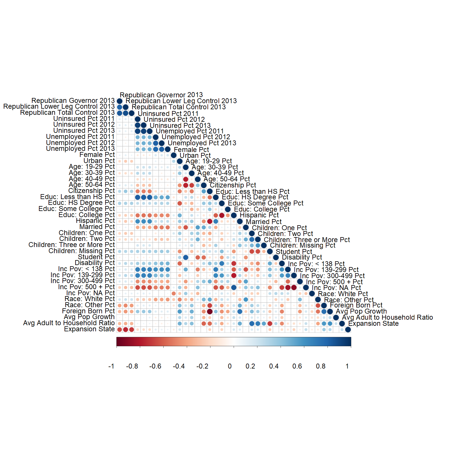
Appendix D Weight Diagnostics
This section contains additional information pertaining to the generation of the balancing weights and their properties.
Table 9 displays each covariate with the targeted level of maximal imbalance when generating approximate balancing weights. All variables and tolerances are measured in percentage points.
Table 10 displays the differences between the weighted mean covariate values of the expansion region and the mean of the non-expansion region for our primary dataset and with the early expansion states excluded (calculated using our the homogeneous covariate adjustments). The weights presented here are for the H-SBW estimator. The values under each column are in the following format: (unweighted difference, weighted difference). “Primary” and “Early excluded” refer to the primary dataset and those that exclude the early expansion states. “Percent” indicates that the differences displayed are in percentage points while “Standardized” indicates that the standardized mean differences are displayed. Additional results are available on request.
Figure 4 shows the weights summed by states for the H-SBW, BC-HSBW, SBW, and BC-HSBW weights on the primary dataset. The positive and negative weights are displayed separately and we standardize the weights to sum to 100. Figure 5 displays the same plot excluding the early expansion states. These plots again show that H-SBW and BC-HSBW more evenly disperses the weights across states relative to SBW and BC-SBW, and also highlights the extent to which the weights extrapolate from each state for the bias-corrected estimators.
We conclude by examining whether the H-SBW weights generated using the unadjusted data balance the adjusted covariates. While these metrics do not reflect the “true” imbalances, the comparison can provide some indication of whether the unadjusted weights are overfitting to noisy covariate measurements. Table 11 compares the imbalances among our pre-treatment outcomes using H-SBW weights generated on our unadjusted dataset applied to the adjusted (homogeneous) dataset. The “Unweighted Difference” column represents the raw difference in means, while the “Weighted Difference” column reflects the weighted difference that we calculate on the unadjusted dataset. The “Homogeneous Diff” column displays the weighted imbalance when applying the H-SBW weights to the dataset using the homogeneous adjustment, and similarly for “Heterogeneous Diff.” The weighted pre-treatment outcomes are approximately one percentage point lower than we desired in the two years prior to treatment using the heterogeneous adjustment, and -0.2 percentage points lower on average using the homogeneous adjustment. On the other hand, the naive difference suggests that the imbalance is only -0.05 percentage points. This result suggests that the unadjusted weights are overfitting to noisy covariates and may give an overly optimistic view of the covariate balance.
| Variable | |
|---|---|
| Uninsured Pct 2011 | 0.05 |
| Uninsured Pct 2012 | 0.05 |
| Uninsured Pct 2013 | 0.05 |
| Unemployed Pct 2011 | 0.15 |
| Unemployed Pct 2012 | 0.15 |
| Unemployed Pct 2013 | 0.15 |
| Avg Pop Growth | 0.50 |
| Avg Adult to Household Ratio | 0.50 |
| Female Pct | 1.00 |
| Age: 19-29 Pct | 1.00 |
| Age: 30-39 Pct | 1.00 |
| Age: 40-49 Pct | 1.00 |
| Age: 50-64 Pct | 1.00 |
| Married Pct | 1.00 |
| Disability Pct | 1.00 |
| Hispanic Pct | 1.00 |
| Race: White Pct | 1.00 |
| Children: One Pct | 1.00 |
| Children: Two Pct | 1.00 |
| Children: Three or More Pct | 1.00 |
| Children: Missing Pct | 1.00 |
| Urban Pct | 2.00 |
| Citizenship Pct | 2.00 |
| Educ: Less than HS Pct | 2.00 |
| Educ: HS Degree Pct | 2.00 |
| Educ: Some College Pct | 2.00 |
| Educ: College Pct | 2.00 |
| Student Pct | 2.00 |
| Inc Pov: 138 Pct | 2.00 |
| Inc Pov: 139-299 Pct | 2.00 |
| Inc Pov: 300-499 Pct | 2.00 |
| Inc Pov: 500 + Pct | 2.00 |
| Inc Pov: NA Pct | 2.00 |
| Race: Other Pct | 2.00 |
| Foreign Born Pct | 2.00 |
| Republican Governor 2013 | 25.00 |
| Republican Lower Leg Control 2013 | 25.00 |
| Republican Total Control 2013 | 25.00 |
(Unweighted difference, Weighted difference)
| Variables | Preferred (Percent) | Preferred (Standardized) | Early excluded (Percent) | Early excluded (Standardized) |
|---|---|---|---|---|
| Age: 19-29 Pct | (-0.34, -0.34) | (-0.05, -0.05) | (-0.62, -0.21) | (-0.09, -0.03) |
| Age: 30-39 Pct | (0.36, 0.17) | (0.1, 0.05) | (-0.04, 0.32) | (-0.01, 0.09) |
| Age: 40-49 Pct | (0.19, -0.3) | (0.06, -0.1) | (-0.01, -0.44) | (0, -0.15) |
| Avg Adult to Household Ratio | (11.29, -0.04) | (0.37, 0) | (3.37, 0.1) | (0.13, 0) |
| Citizenship Pct | (-3.61, -1.59) | (-0.33, -0.15) | (-0.24, -1.45) | (-0.03, -0.16) |
| Disability Pct | (-1.45, 0.52) | (-0.27, 0.1) | (-0.17, 0.63) | (-0.03, 0.11) |
| Educ: HS Degree Pct | (-3.37, 0.54) | (-0.32, 0.05) | (-1.02, 0.64) | (-0.1, 0.06) |
| Educ: Less than HS Pct | (-0.37, 0.83) | (-0.04, 0.1) | (-1.22, 0.76) | (-0.16, 0.1) |
| Educ: Some College Pct | (-0.35, 0.4) | (-0.05, 0.06) | (0.36, 0.57) | (0.05, 0.08) |
| Female Pct | (-0.34, -0.64) | (-0.16, -0.3) | (-0.25, -1) | (-0.12, -0.48) |
| Foreign Born Pct | (7.6, 2) | (0.42, 0.11) | (1.02, 2) | (0.07, 0.13) |
| Uninsured Pct 2011 | (-3.08, 0.05) | (-0.28, 0) | (-3.51, -0.05) | (-0.34, 0) |
| Uninsured Pct 2012 | (-3, -0.05) | (-0.27, 0) | (-3.4, 0.05) | (-0.33, 0) |
| Uninsured Pct 2013 | (-2.99, -0.05) | (-0.27, 0) | (-3.45, -0.05) | (-0.34, 0) |
| Hispanic Pct | (4.46, 1) | (0.2, 0.04) | (-1.35, 1) | (-0.07, 0.05) |
| Inc Pov: 138 Pct | (-2.05, 0.63) | (-0.19, 0.06) | (-1.33, 0.12) | (-0.12, 0.01) |
| Inc Pov: 139-299 Pct | (-2.45, 0.65) | (-0.35, 0.09) | (-1.53, 0.5) | (-0.23, 0.08) |
| Inc Pov: 300-499 Pct | (-0.59, -0.18) | (-0.12, -0.04) | (0.28, -0.18) | (0.06, -0.04) |
| Inc Pov: 500 + Pct | (5.58, -1.3) | (0.35, -0.08) | (2.9, -1.23) | (0.2, -0.08) |
| Married Pct | (-0.76, -0.43) | (-0.07, -0.04) | (-0.21, -0.53) | (-0.02, -0.05) |
| Children: Missing Pct | (-3.25, -1) | (-0.36, -0.11) | (-1.99, -0.1) | (-0.21, -0.01) |
| Children: One Pct | (0.7, -0.14) | (0.25, -0.05) | (0.11, -0.31) | (0.04, -0.12) |
| Avg Pop Growth | (-0.09, -0.21) | (-0.07, -0.18) | (-0.26, -0.19) | (-0.22, -0.16) |
| Race: White Pct | (-4.02, 1) | (-0.16, 0.04) | (0.09, 1) | (0, 0.04) |
| Republican Governor 2013 | (-64.78, -25) | (-1.28, -0.5) | (-54.46, -24.87) | (-1.02, -0.47) |
| Republican Lower Leg Control 2013 | (-74.72, -25) | (-1.69, -0.57) | (-56.67, -23.6) | (-1.12, -0.47) |
| Republican Total Control 2013 | (-71.3, -25) | (-1.45, -0.51) | (-56.47, -25) | (-1.02, -0.45) |
| Student Pct | (0.25, -0.5) | (0.04, -0.08) | (0.11, -0.25) | (0.02, -0.04) |
| Children: Three or More Pct | (0, -0.21) | (0, -0.08) | (-0.17, -0.26) | (-0.07, -0.11) |
| Children: Two Pct | (0.76, -0.31) | (0.23, -0.09) | (0.17, -0.37) | (0.05, -0.12) |
| Unemployed Pct 2011 | (0.82, 0.15) | (0.18, 0.03) | (0.68, 0.15) | (0.15, 0.03) |
| Unemployed Pct 2012 | (0.63, -0.03) | (0.14, -0.01) | (0.47, -0.03) | (0.11, -0.01) |
| Unemployed Pct 2013 | (0.42, -0.15) | (0.11, -0.04) | (0.22, -0.15) | (0.06, -0.04) |
| Urban Pct | (8.28, -2) | (0.26, -0.06) | (2.79, -2) | (0.08, -0.06) |
-
The values displayed in each cell are the (unweighted, weighted) differences. The columns containing “Standardized” reflect the standardized mean differences while “percent” indicates the mean differences in percentage points. The columns containing “Preferred” indicate that this is for our primary analysis while “Early excluded” is for our analysis that excludes the early expansion states.
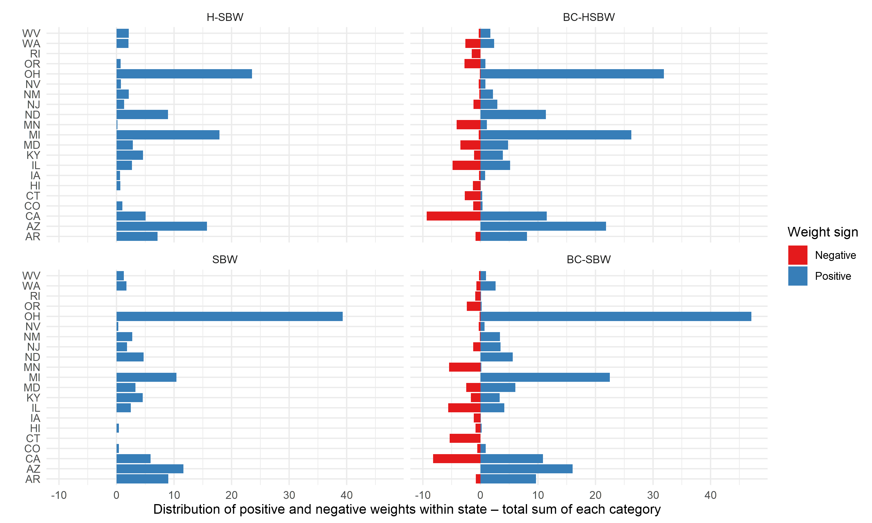
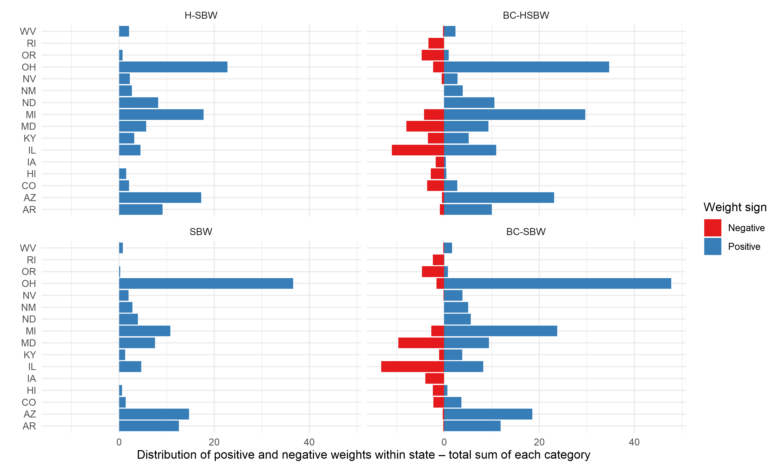
(primary dataset)
| Variable | Unweighted Difference | Weighted Difference | Homogeneous Difference | Heterogeneous Difference |
|---|---|---|---|---|
| Uninsured Pct 2011 | -3.09 | -0.05 | -0.11 | 0.92 |
| Uninsured Pct 2012 | -2.99 | -0.05 | -0.21 | -1.06 |
| Uninsured Pct 2013 | -3.00 | -0.05 | -0.38 | -0.93 |
Appendix E Additional Results
This section contains additional results that were not displayed in the main paper.
Tables 12 and 13 presents the full model validation results that also include estimators using the Oaxaca-Blinder OLS and GLS weights (see, e.g, Kline (2011)). The first table only presents the mean error and RMSE, with rows ordered by RMSE for each dataset, while the second table contains the errors for each individual year and the RMSE, with rows ordered by RMSE on the primary dataset. We find that the OLS and GLS estimators perform quite poorly, again showing that the cost of extrapolation is quite high in our application.
Table 14 displays the point estimates and confidence intervals from all estimators we considered, including those using the “heterogeneous adjustment.”
Figure 6(a) displays the change in our estimator when removing each state for all four of our estimators on the adjusted dataset (“homogeneous”) and the unadjusted dataset (“unadjusted”) for the primary dataset. Figure 7(a) displays the same information when excluding the early expansion states.
Our final two tables (Tables 15 and 16) display each point estimate associated with each estimator in the leave-one-state-out jackknife.
| Primary dataset | Early expansion excluded | ||||||
|---|---|---|---|---|---|---|---|
| Sigma estimate | Estimator | Mean Error | RMSE | Sigma estimate | Estimator | Mean Error | RMSE |
| Homogeneous | SBW | -0.20 | 0.20 | Homogeneous | BC-HSBW | -0.02 | 0.07 |
| Homogeneous | H-SBW | -0.23 | 0.23 | Homogeneous | BC-SBW | -0.03 | 0.12 |
| Heterogeneous | SBW | -0.27 | 0.27 | Heterogeneous | BC-HSBW | -0.08 | 0.14 |
| Heterogeneous | H-SBW | -0.35 | 0.36 | Heterogeneous | BC-SBW | -0.07 | 0.15 |
| Homogeneous | BC-SBW | -0.39 | 0.39 | Homogeneous | H-SBW | 0.01 | 0.25 |
| Heterogeneous | BC-SBW | -0.42 | 0.42 | Homogeneous | SBW | 0.07 | 0.26 |
| Unadjusted | SBW | -0.56 | 0.56 | Heterogeneous | SBW | 0.04 | 0.28 |
| Unadjusted | H-SBW | -0.57 | 0.57 | Heterogeneous | H-SBW | -0.04 | 0.29 |
| Homogeneous | BC-HSBW | -0.58 | 0.58 | Heterogeneous | GLS | -0.02 | 0.29 |
| Heterogeneous | BC-HSBW | -0.63 | 0.63 | Heterogeneous | OLS | -0.14 | 0.39 |
| Unadjusted | BC-SBW | -0.88 | 0.88 | Unadjusted | SBW | -0.37 | 0.42 |
| Unadjusted | OLS | -0.88 | 0.88 | Unadjusted | H-SBW | -0.43 | 0.46 |
| Unadjusted | GLS | -0.89 | 0.89 | Unadjusted | BC-HSBW | -0.60 | 0.60 |
| Unadjusted | BC-HSBW | -0.96 | 0.96 | Unadjusted | GLS | -0.61 | 0.63 |
| Homogeneous | OLS | -1.48 | 1.50 | Unadjusted | OLS | -0.70 | 0.71 |
| Homogeneous | GLS | -1.60 | 1.61 | Unadjusted | BC-SBW | -0.70 | 0.71 |
| Heterogeneous | GLS | -9.39 | 12.47 | Homogeneous | GLS | 0.28 | 0.98 |
| Heterogeneous | OLS | -11.88 | 16.21 | Homogeneous | OLS | 0.02 | 1.10 |
| Primary dataset | Early expansion excluded | ||||||
|---|---|---|---|---|---|---|---|
| Sigma estimate | Estimator | 2012 error | 2013 error | RMSE | 2012 error | 2013 error | RMSE |
| Homogeneous | SBW | -0.18 | -0.22 | 0.20 | 0.32 | -0.18 | 0.26 |
| Homogeneous | H-SBW | -0.24 | -0.21 | 0.23 | 0.26 | -0.24 | 0.25 |
| Heterogeneous | SBW | -0.25 | -0.30 | 0.27 | 0.31 | -0.24 | 0.28 |
| Heterogeneous | H-SBW | -0.32 | -0.39 | 0.36 | 0.25 | -0.32 | 0.29 |
| Homogeneous | BC-SBW | -0.42 | -0.35 | 0.39 | 0.09 | -0.15 | 0.12 |
| Heterogeneous | BC-SBW | -0.45 | -0.39 | 0.42 | 0.07 | -0.21 | 0.15 |
| Unadjusted | SBW | -0.50 | -0.61 | 0.56 | -0.18 | -0.56 | 0.42 |
| Unadjusted | H-SBW | -0.52 | -0.61 | 0.57 | -0.26 | -0.60 | 0.46 |
| Homogeneous | BC-HSBW | -0.53 | -0.62 | 0.58 | 0.05 | -0.09 | 0.07 |
| Heterogeneous | BC-HSBW | -0.53 | -0.72 | 0.63 | 0.03 | -0.19 | 0.14 |
| Unadjusted | BC-SBW | -0.82 | -0.93 | 0.88 | -0.55 | -0.84 | 0.71 |
| Unadjusted | OLS | -0.91 | -0.84 | 0.88 | -0.81 | -0.59 | 0.71 |
| Unadjusted | GLS | -0.87 | -0.91 | 0.89 | -0.78 | -0.44 | 0.63 |
| Unadjusted | BC-HSBW | -0.93 | -0.99 | 0.96 | -0.61 | -0.58 | 0.60 |
| Homogeneous | OLS | -1.75 | -1.21 | 1.50 | 1.12 | -1.08 | 1.10 |
| Homogeneous | GLS | -1.76 | -1.45 | 1.61 | 1.22 | -0.66 | 0.98 |
| Heterogeneous | GLS | -1.18 | -17.60 | 12.47 | 0.27 | -0.32 | 0.29 |
| Heterogeneous | OLS | -0.85 | -22.90 | 16.21 | 0.22 | -0.50 | 0.39 |
| Primary dataset | Early expansion excluded | ||||
|---|---|---|---|---|---|
| Weight type | Adjustment | Estimate (95% CI) | Difference | Estimate (95% CI) | Difference |
| H-SBW | Homogeneous | -2.33 (-3.54, -1.11) | 0.01 | -2.09 (-3.24, -0.94) | 0.19 |
| H-SBW | Heterogeneous | -2.24 (-3.47, -1.00) | 0.10 | -2.06 (-3.36, -0.77) | 0.22 |
| H-SBW | Unadjusted | -2.34 (-2.88, -1.79) | - | -2.28 (-2.87, -1.70) | - |
| BC-HSBW | Homogeneous | -2.05 (-3.30, -0.80) | 0.17 | -1.94 (-3.27, -0.61) | 0.28 |
| BC-HSBW | Heterogeneous | -1.98 (-3.21, -0.75) | 0.24 | -1.93 (-3.55, -0.32) | 0.29 |
| BC-HSBW | Unadjusted | -2.22 (-2.91, -1.52) | - | -2.22 (-3.14, -1.31) | - |
| SBW | Homogeneous | -2.35 (-3.76, -0.95) | 0.04 | -2.05 (-3.19, -0.91) | 0.16 |
| SBW | Heterogeneous | -2.28 (-3.58, -0.98) | 0.11 | -2.03 (-3.35, -0.72) | 0.18 |
| SBW | Unadjusted | -2.39 (-2.99, -1.79) | - | -2.21 (-2.75, -1.68) | - |
| BC-SBW | Homogeneous | -2.07 (-3.14, -1.00) | 0.13 | -1.99 (-3.33, -0.66) | 0.23 |
| BC-SBW | Heterogeneous | -2.00 (-3.07, -0.92) | 0.20 | -2.00 (-3.65, -0.34) | 0.23 |
| BC-SBW | Unadjusted | -2.19 (-2.94, -1.45) | - | -2.23 (-3.12, -1.33) | - |
-
Note: “Difference” column reflects difference between adjusted and unadjusted estimators
-
Note: Confidence intervals are estimated using the leave-one-state-out jackknife and quantiles from t-distribution with degrees of freedom.
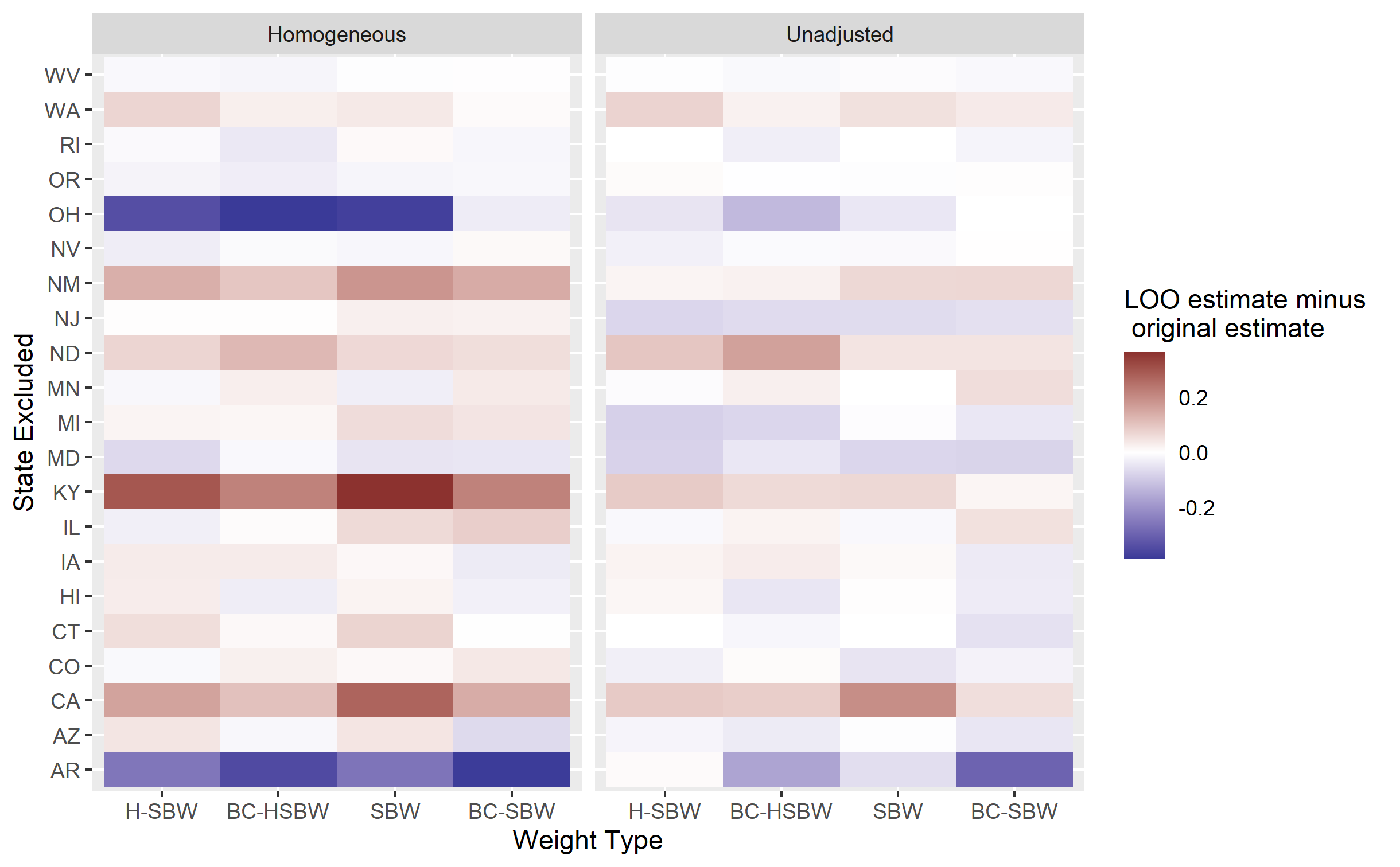
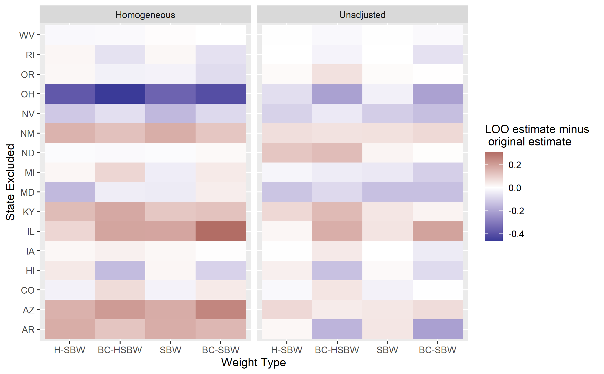
| Homogeneous | Heterogeneous | Unadjusted | ||||||||||
|---|---|---|---|---|---|---|---|---|---|---|---|---|
| Left out state | BC-HSBW | BC-SBW | H-SBW | SBW | BC-HSBW | BC-SBW | H-SBW | SBW | BC-HSBW | BC-SBW | H-SBW | SBW |
| All | -2.05 | -2.07 | -2.33 | -2.35 | -1.98 | -2.00 | -2.24 | -2.28 | -2.22 | -2.19 | -2.34 | -2.39 |
| AR | -2.40 | -2.45 | -2.59 | -2.61 | -2.30 | -2.36 | -2.46 | -2.52 | -2.38 | -2.49 | -2.33 | -2.45 |
| AZ | -2.06 | -2.14 | -2.28 | -2.31 | -2.02 | -2.06 | -2.26 | -2.25 | -2.25 | -2.24 | -2.35 | -2.39 |
| CA | -1.94 | -1.93 | -2.17 | -2.08 | -1.96 | -1.90 | -2.12 | -2.04 | -2.13 | -2.14 | -2.24 | -2.19 |
| CO | -2.02 | -2.03 | -2.34 | -2.34 | -2.00 | -1.98 | -2.34 | -2.34 | -2.21 | -2.22 | -2.36 | -2.44 |
| CT | -2.04 | -2.07 | -2.27 | -2.28 | -1.98 | -2.00 | -2.20 | -2.22 | -2.23 | -2.25 | -2.34 | -2.39 |
| HI | -2.08 | -2.09 | -2.30 | -2.33 | -2.01 | -2.03 | -2.20 | -2.26 | -2.26 | -2.23 | -2.32 | -2.39 |
| IA | -2.01 | -2.10 | -2.29 | -2.34 | -1.93 | -2.04 | -2.18 | -2.26 | -2.19 | -2.23 | -2.31 | -2.38 |
| IL | -2.04 | -1.98 | -2.36 | -2.29 | -2.00 | -1.94 | -2.31 | -2.26 | -2.20 | -2.14 | -2.35 | -2.40 |
| KY | -1.83 | -1.85 | -2.03 | -1.99 | -1.79 | -1.82 | -1.99 | -1.97 | -2.15 | -2.18 | -2.25 | -2.32 |
| MD | -2.06 | -2.11 | -2.40 | -2.40 | -2.02 | -2.04 | -2.32 | -2.33 | -2.26 | -2.27 | -2.42 | -2.46 |
| MI | -2.03 | -2.02 | -2.31 | -2.29 | -1.96 | -1.88 | -2.23 | -2.16 | -2.29 | -2.24 | -2.42 | -2.39 |
| MN | -2.02 | -2.03 | -2.34 | -2.38 | -1.99 | -1.96 | -2.30 | -2.33 | -2.19 | -2.14 | -2.34 | -2.39 |
| ND | -1.93 | -2.01 | -2.26 | -2.29 | -1.85 | -1.93 | -2.17 | -2.21 | -2.05 | -2.15 | -2.24 | -2.34 |
| NJ | -2.04 | -2.04 | -2.32 | -2.33 | -2.01 | -2.01 | -2.28 | -2.30 | -2.28 | -2.25 | -2.41 | -2.45 |
| NM | -1.95 | -1.92 | -2.19 | -2.17 | -1.94 | -1.91 | -2.20 | -2.19 | -2.19 | -2.13 | -2.32 | -2.32 |
| NV | -2.06 | -2.06 | -2.36 | -2.37 | -1.99 | -1.99 | -2.27 | -2.31 | -2.23 | -2.19 | -2.36 | -2.40 |
| OH | -2.43 | -2.10 | -2.67 | -2.72 | -2.41 | -2.20 | -2.67 | -2.64 | -2.34 | -2.19 | -2.38 | -2.43 |
| OR | -2.08 | -2.08 | -2.35 | -2.37 | -2.05 | -2.05 | -2.33 | -2.36 | -2.22 | -2.19 | -2.33 | -2.39 |
| RI | -2.09 | -2.08 | -2.34 | -2.34 | -2.01 | -2.01 | -2.22 | -2.26 | -2.25 | -2.21 | -2.34 | -2.39 |
| WA | -2.02 | -2.06 | -2.26 | -2.32 | -1.99 | -2.03 | -2.24 | -2.31 | -2.19 | -2.16 | -2.26 | -2.34 |
| WV | -2.07 | -2.07 | -2.34 | -2.36 | -2.00 | -2.01 | -2.24 | -2.29 | -2.23 | -2.21 | -2.34 | -2.40 |
-
•
Note: Row labeled “All” reflects the original estimate
| Homogeneous | Heterogeneous | Unadjusted | ||||||||||
|---|---|---|---|---|---|---|---|---|---|---|---|---|
| Left out state | BC-HSBW | BC-SBW | H-SBW | SBW | BC-HSBW | BC-SBW | H-SBW | SBW | BC-HSBW | BC-SBW | H-SBW | SBW |
| All | -1.94 | -1.99 | -2.09 | -2.05 | -1.93 | -2.00 | -2.06 | -2.03 | -2.22 | -2.23 | -2.28 | -2.21 |
| AR | -1.82 | -1.85 | -1.92 | -1.88 | -1.71 | -1.73 | -1.77 | -1.75 | -2.39 | -2.44 | -2.27 | -2.16 |
| AZ | -1.73 | -1.74 | -1.93 | -1.88 | -1.64 | -1.66 | -1.85 | -1.81 | -2.18 | -2.15 | -2.21 | -2.17 |
| CO | -1.87 | -1.95 | -2.12 | -2.08 | -1.86 | -1.92 | -2.09 | -2.00 | -2.17 | -2.23 | -2.30 | -2.24 |
| HI | -2.09 | -2.09 | -2.05 | -2.03 | -2.08 | -2.09 | -2.04 | -1.95 | -2.36 | -2.30 | -2.25 | -2.20 |
| IA | -1.91 | -1.99 | -2.07 | -2.03 | -1.85 | -1.95 | -2.01 | -1.98 | -2.18 | -2.27 | -2.28 | -2.21 |
| IL | -1.75 | -1.68 | -2.01 | -1.86 | -1.62 | -1.56 | -1.94 | -1.79 | -2.06 | -2.03 | -2.27 | -2.16 |
| KY | -1.76 | -1.87 | -1.95 | -1.93 | -1.70 | -1.85 | -1.89 | -1.89 | -2.08 | -2.20 | -2.20 | -2.16 |
| MD | -1.98 | -1.96 | -2.24 | -2.09 | -1.85 | -1.87 | -2.07 | -1.96 | -2.31 | -2.36 | -2.41 | -2.35 |
| MI | -1.86 | -1.95 | -2.07 | -2.09 | -1.97 | -1.94 | -2.14 | -1.97 | -2.26 | -2.33 | -2.31 | -2.26 |
| ND | -1.95 | -1.98 | -2.10 | -2.06 | -1.86 | -1.94 | -1.95 | -1.97 | -2.09 | -2.22 | -2.17 | -2.19 |
| NM | -1.81 | -1.88 | -1.94 | -1.88 | -1.88 | -1.89 | -1.98 | -1.86 | -2.17 | -2.15 | -2.22 | -2.15 |
| NV | -2.01 | -2.08 | -2.21 | -2.20 | -1.92 | -2.00 | -2.10 | -2.01 | -2.27 | -2.36 | -2.38 | -2.32 |
| OH | -2.40 | -2.40 | -2.48 | -2.41 | -2.45 | -2.48 | -2.49 | -2.47 | -2.43 | -2.43 | -2.36 | -2.25 |
| OR | -1.97 | -2.07 | -2.07 | -2.08 | -2.00 | -2.05 | -2.08 | -1.97 | -2.16 | -2.22 | -2.27 | -2.21 |
| RI | -2.00 | -2.06 | -2.07 | -2.03 | -2.00 | -2.05 | -2.08 | -2.01 | -2.25 | -2.29 | -2.28 | -2.21 |
| WV | -1.95 | -1.99 | -2.11 | -2.04 | -1.91 | -1.98 | -2.07 | -2.03 | -2.24 | -2.24 | -2.29 | -2.22 |
-
•
Note: Row labeled “All” reflects the original estimate
Appendix F Simulation Study
This final section presents simulation results evaluating the performance of our proposed estimators in an idealized setting where the outcome model and measurement error models are known. The first subsection outlines our simulation study. The second subsection presents selected results, including the bias, mean-square error, and coverage rates for our proposed estimators and variance estimates. The final subsection provides additional results analyzing the performance of H-SBW and our proposed variance estimator absent measurement error.
F.1 Study design
For our simulations we generate populations of states, each with CPUMAs, so that we obtain a population of CPUMAs. We draw so that the average number of regions per state is approximately 20. We then generate a 3-dimensional covariate vector :
| (64) | |||
| (65) |
Define . Let be the j-th diagonal element of . Across all simulations, we fix this number to be constant and equal to 2 (i.e. ). We also fix the off-diagonal elements of both and to be equal and so that . Finally, let denote the within-state correlation of the observations (i.e. for ). We set this value to be equal for all covariates, so that , but vary this parameter across simulations.
We then generate outcomes according to the model:
where is a block-diagonal matrix representing homoskedastic and equicorrelated errors outlined below.
| (66) | ||||
| (67) |
In other words represents the variance component from a state-level random effect and represents a variance component from a CPUMA-level random effect, as described in the main paper.
We next generate our noisy outcome and covariate estimates :
We allow to either be constant or a function of the sample size of an underlying survey that generates the estimate. In the latter case we simulate these sample sizes . We calculate that satisfies the following equality: . This reflects the model assumed in the “heterogeneous adjustment.” We also define as the expected value of :
We then define parameter :
We consider different values of throughout our simulations. This parameter reflects the extent of the measurement error, with meaning that the covariates are measured without error, and the noise increasing as goes to zero.
Define . represents the within-state correlation of the outcome model errors given the true covariates , including the measurement errors in the outcome. We fix this to be 0.25 for our primary simulation results. We caveat that only represents an optimal value in a setting without measurement error. This is due to the contribution of additional terms in the variance of the estimator from the noisy covariate measurements.
We then consider all 18 combinations of the following parameters:
-
•
-
•
-
•
For each parameterization we take 1000 random samples of size states (with total CPUMAs that average around 450). For each sample we estimate a series of H-SBW weights that set and the target . Let denote the assumed in the H-SBW objective. We generate weights for all combinations of input datasets and correlation-parameters :
-
•
, , , , }
-
•
We estimate the variance for each estimator using the leave-one-state-out jackknife, described in Section 3.
Note: for we use the empirical covariance matrix of , the estimated means , and , where we draw from . In other words, when averaged together we assume that have a fairly precise estimate of .
F.2 Selected results
We present the results where the “heterogeneous adjustment” model is correct. The results for the homoskedastic measurement errors are quite similar and we observe in the text where they differ. Figure 8 displays the bias associated with each estimator. From left to right the panels reflect different values of : the left-most panels have the most measurement error while the right-most panels have the least. From top to bottom the panels reflect different values of : the top-most panel has no correlation structure among the covariates, while the bottom-most panels are more highly correlated within state. Within each panel we organize the results by the input covariate set: represents the estimators generated without any covariate adjustment; reflects estimators generated on the true covariates; “Xhat-het” represents the heterogeneous adjustment (), “Xhat-hom” represents the homogeneous adjustment (), and “Xhat-cor” represents the correlated adjustment (), described in Appendix B. The estimators are colored by the assumed value of in the H-SBW objective, where is equivalent to SBW. Across all of the present simulations, we set equal to 0.25.
We highlight two general results. First, if we know the true values of , all of our estimators are unbiased. Second, balancing on results in bias. This bias increases as decreases, and, when the covariates are dependent, increases with . These results are consistent with our propositions in Appendices A.1 and A.2.
When attempting to mitigate this bias by using some estimate of , balancing on , , or results in approximately unbiased estimates for all values of when the covariates uncorrelated. When are correlated across observations, setting results in biased estimates for or , where the bias increases with . The SBW estimators remain approximately unbiased, even when the data are correlated. We speculate in Remark 10 why this may be the case. In settings where the estimators using that remain approximately unbiased. However, when even these estimators appear to have some bias. In further investigations (results not displayed but available on request), this bias decreases with the number of states. Regardless of the adjustment set, all biases on the adjusted datasets are smaller in absolute magnitude than the corresponding biases associated with estimators that naively balance .
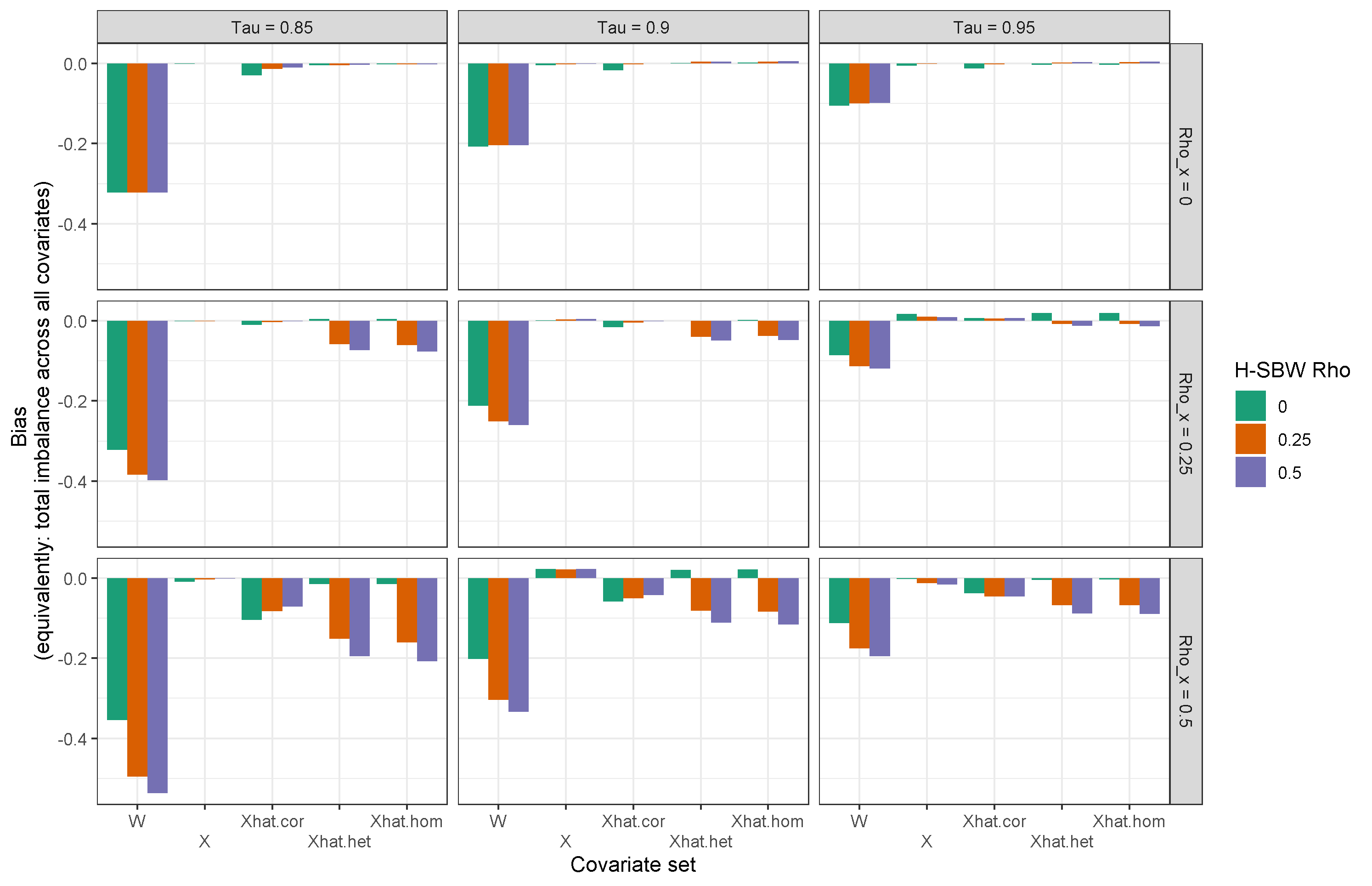
All of these simulations had heterogeneous measurement error. When examining the results when the errors are homoskedastic we find that the estimators that balance on have a small bias even when or . Assuming this model is correct when it is not appears to have some cost. This may help explain the slightly worse performance we found when using the heterogeneous adjustment in our validation study in Section 4.
Figure 9 displays the variance associated with these same estimators. Throughout we obtain modest reductions in variance as we increase . Choosing either or gives similar reductions relative to choosing (again equivalent to SBW). These variance reductions may increase if we increased , which we fix in this simulation study to be 0.25. For example, Section F.3, Figure 13, considers a wider range of parameterizations of in a context without measurement error, and shows that larger variance reductions are possible when is higher. Admittedly, these settings may be unlikely in practice.262626In the setting without measurement error represents the optimal value.
These results also show that balancing on can lead to a much more variable estimate, particularly when the covariates have larger within-state correlations. Only in the setting with uncorrelated covariates and little measurement error does the variability induced by this adjustment appears to have less cost.
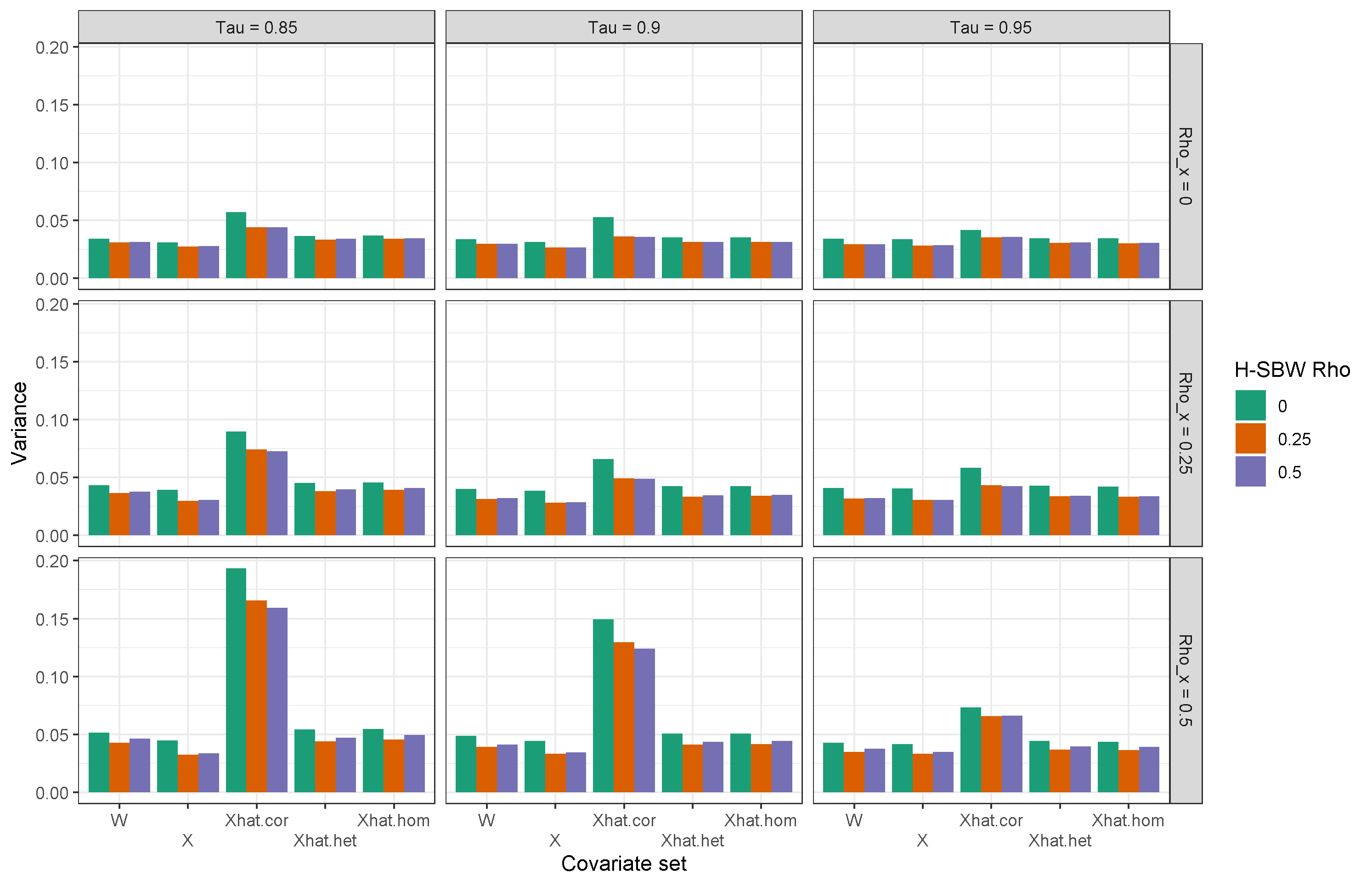
Figure 10 displays the MSE of these estimators. The estimators generated on have larger MSE, largely driven by the increase in variability we observed previously. Despite the increase in bias for H-SBW with or we still often find modest MSE reductions when using H-SBW relative to SBW. This appears more likely as the magnitude of the measurement error decreases and/or the within-state correlation decreases (i.e. moving towards the top-right of the plot). Whether an MSE improvement is possible also depends on : if we were to set , we would expect the MSE of these estimators to increase for all estimators as increases, even when we observe (see also Section F.3). The results are similar when considering homoskedastic measurement errors, though the space where we see MSE improvements for H-SBW relative to SBW on the uncorrelated adjustments appears to increase slightly (results available on request).
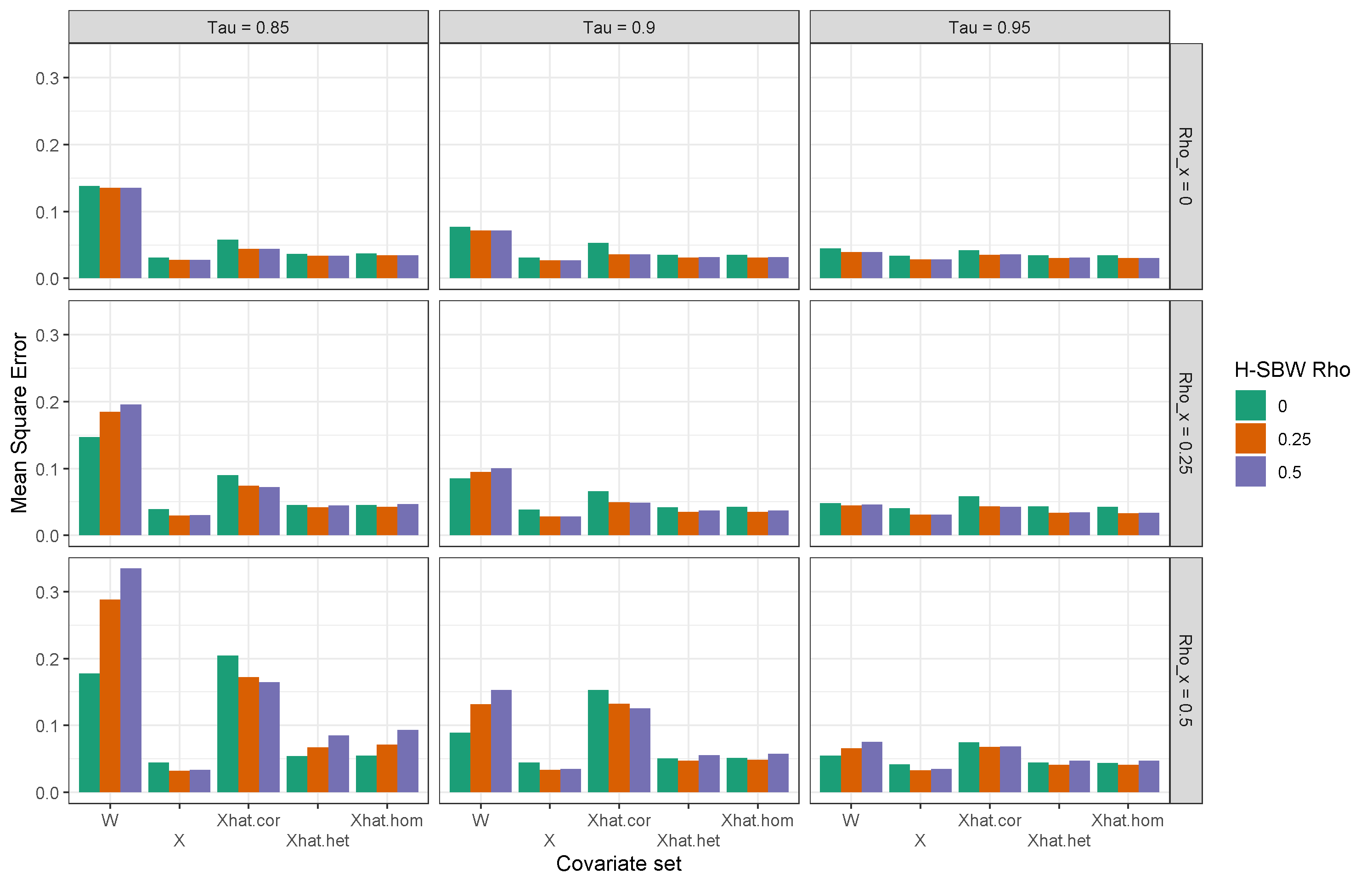
We next evaluate the performance of the leave-one-state-out jackknife procedure and evaluate confidence interval coverage (for 95% confidence intervals) and length, and display these results in Figures 11 and 12. We use the standard normal quantiles to generate confidence intervals throughout.
Figure 11 shows that using SBW () we obtain approximately nominal coverage rates across all specifications that use or some version of . However we fail to ever achieve nominal coverage rates when balancing on . Even when the amount of measurement error is small () we only obtain at best slightly below 90 percent coverage rates. Confidence interval coverage appears to deteriorate as we increase , even when balancing on the true covariates .272727This is consistent with results in Cameron, Gelbach and Miller (2008). Unsurprisingly the rates worsen for estimators generated on and in the settings where we found the highest bias. We also obtain slightly less than desired rates for estimators using . This may be due to the fact that we do not use any degrees-of-freedom adjustment for our confidence intervals (we examine this further in Section F.3). On the other hand, coverage rates are accurate or conservative for estimators generated on . The positive bias of the jackknife variance estimates appears to drive this result.282828We almost always find a positive or negligible bias for the unscaled jackknife variance estimates, consistent with Proposition 5.
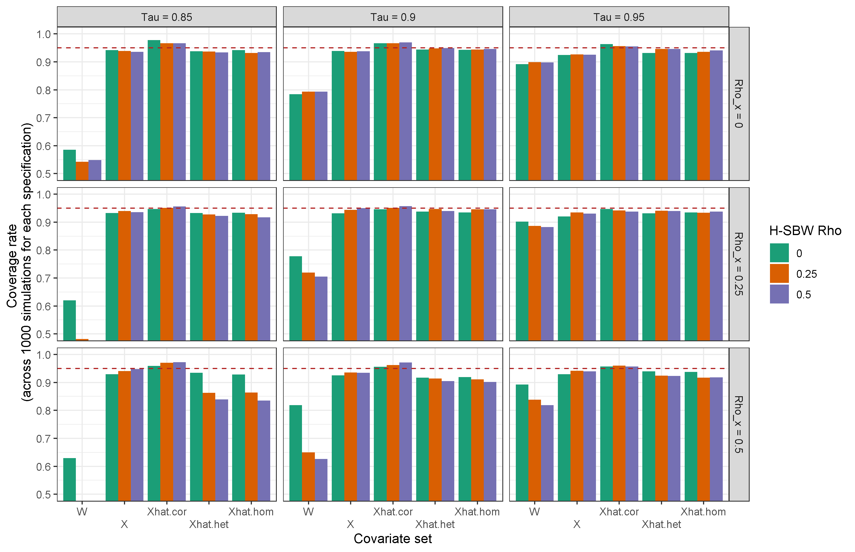
Figure 12 compares the mean confidence interval lengths using the leave-one-state-out jackknife. The H-SBW estimator is associated with slightly more precise estimates, reflecting that the estimators have decreased variability under our assumed correlation structures. We again see that even when we choose sub-optimally we obtain more precise inferences than when using SBW. This suggests benefits to using H-SBW even when our estimate of is inaccurate. As the previous results would suggest, the confidence intervals using are quite large. The results are similar when considering homoskedastic measurement errors.
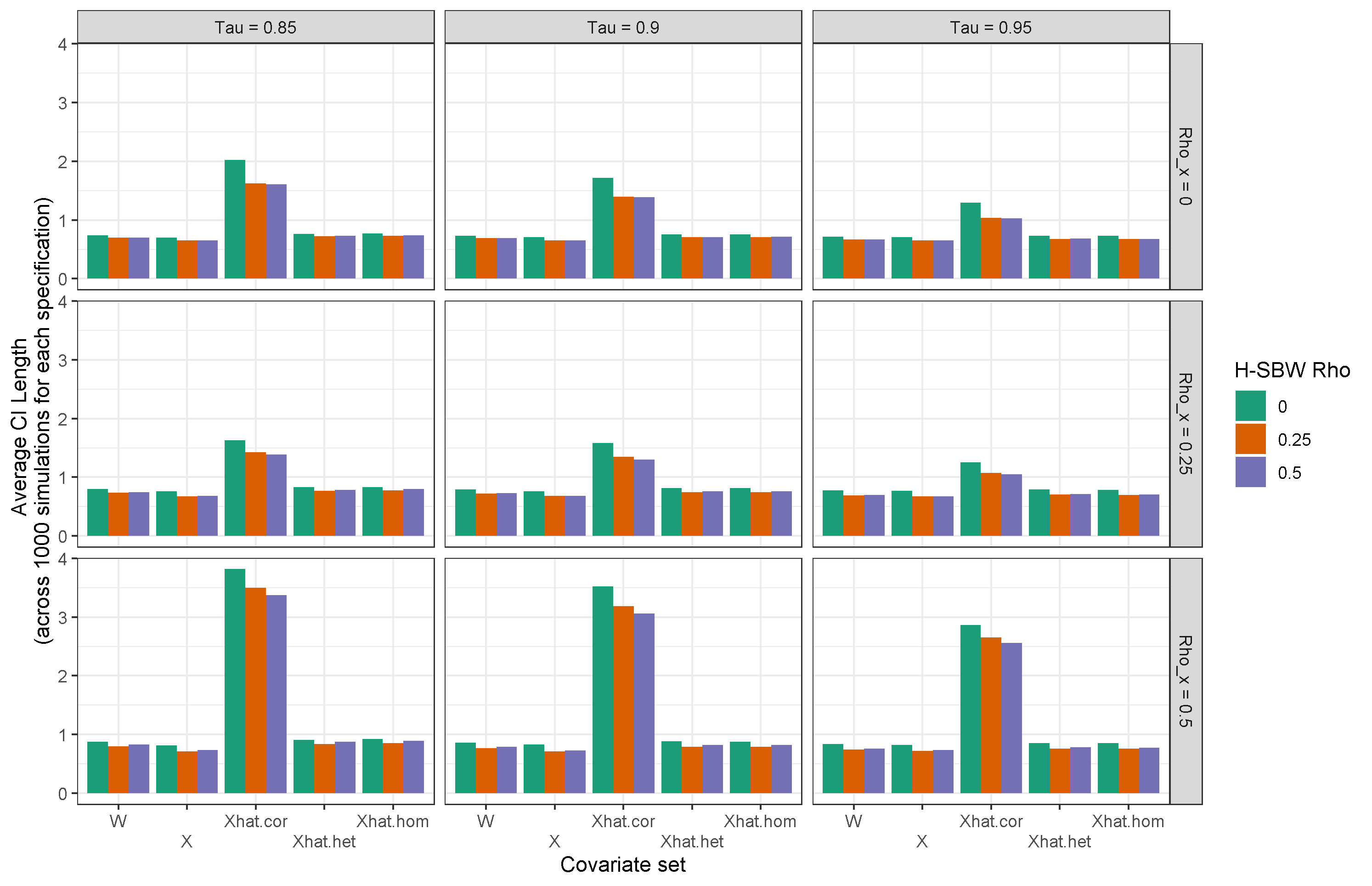
We emphasize five takeaways from this simulation study. First, the variance improvements of SBW relative to H-SBW are likely modest. That said, the extent to which we can improve on SBW also depend on , which we fix in this study, and these improvements can be greater as increases, which we explore more in Section F.3 below.292929They also depend on how varies across states. We draw from only one distribution throughout our simulations. Second, H-SBW can increase the bias of our proposed estimators in the context of measurement error and dependent data. However, the bias is generally small relative to the bias of balancing on the noisy covariate measurements , and MSE improvements using H-SBW are still possible relative to SBW with the simple covariate adjustments ( or ). Third, despite the improved theoretic properties, accounting for the correlation in the data when using H-SBW (i.e. balancing on and the data are measured with error) may not be worth the cost in variance given the sample size of states that we consider here. Fourth, we find no evidence that the “heterogeneous adjustment” improves our subsequent estimates even when it reflects the true model. This adjustment may even induce bias when the model is incorrect.303030This finding may in part reflect the distribution of sample sizes we generated, which we took to be uniform. Perhaps with a different distribution these results would differ. Finally, confidence interval coverage when using the leave-one-state-out jackknife variance estimates give close to nominal coverage rates for our unbiased estimators – even when using the standard normal quantiles in a setting with 25 states.
This simulation study assumes throughout that we know the true data generating model for the outcome and that are data are gaussian. Because in practice we would not have such knowledge, this study complements our validation study in Section 4, which has more direct bearing on understanding how these estimators might perform in an applied setting.
F.3 Additional results: H-SBW without measurement error
We consider additional simulations for the setting where is known and the outcome model follows homoskedastic but possibly correlated errors. For these results we only vary , and fix throughout.
Figure 13 displays the empirical variance of the H-SBW estimators averaged over 1000 simulations. Each panel reflects different values of , while the x-axis throughout displays the assumed value of in the H-SBW objective. The red bars indicate when is optimally selected, . This selection corresponds with the lowest variance estimator as we expect. Consistent with our previous results, when any assumed improves the variance of the resulting estimator relative to SBW. This requires in general that our assumed correlation structure of the error terms is correct.
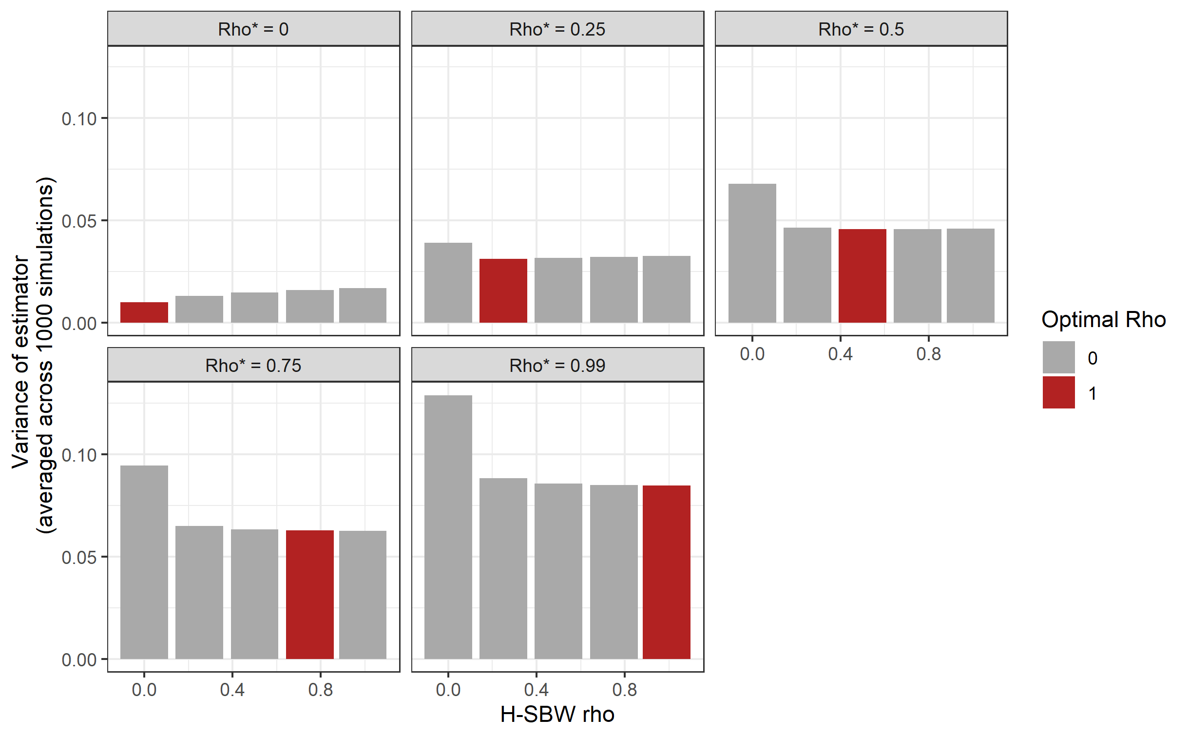
We conclude by examining the confidence interval coverage for the leave-one-state-out-jackknife. Figure 14 displays the results. Consistent with our previous findings we obtain slightly less than nominal coverage rates, particularly when is small. This slight undercoverage is likely due in part to our use of standard normal quantiles to generate confidence intervals.313131Consistent with Proposition 5 and the previous results we again find that the unscaled variance estimates are all either positively or negligibly biased. Interestingly, coverage appears to improve when setting even when . We speculate that by more evenly dispersing the weights across states, H-SBW may be increasing the effective degrees of freedom of the estimator (see, e.g., Cameron and Miller (2015)), illustrating another potential benefit of this approach. Analyzing the theoretic properties of these variances estimators in this setting is beyond the scope of the present study but would provide interesting future work.