Bare Demo of IEEEtran.cls
for IEEE Journals
Dual-Robust Integrated Sensing and Communication: Beamforming under CSI Imperfection and Location Uncertainty
Abstract
A dual-robust design of beamforming is investigated in an integrated sensing and communication (ISAC) system. Existing research on robust ISAC waveform design, while proposing solutions to imperfect channel state information (CSI), generally depends on prior knowledge of the target’s approximate location to design waveforms. This approach, however, limits the precision in sensing the target’s exact location. In this paper, considering both CSI imperfection and target location uncertainty, a novel framework of joint robust optimization is proposed by maximizing the weighted sum of worst-case data rate and beampattern gain. To address this challenging problem, we propose an efficient two-layer iteration algorithm based on S-Procedure and convex hull. Finally, numerical results verify the effectiveness and performance improvement of our dual-robust algorithm, as well as the trade-off between communication and sensing performance.
Index Terms:
Integrated sensing and communication, dual functional radar and communication, robust beamforming, optimization.I Introduction
Integrated sensing and communication (ISAC) has emerged as a promising technology in future mobile networks. In numerous application scenarios, including internet-of-vehicles, smart homes, and environmental monitoring, the incorporation of environmental sensing into the communication stage has significantly evolved, enhancing overall system functionality and efficiency. [1]. With an integrated hardware platform for both sensing and communication, ISAC systems offers mutual benefits to both functionalities, resulting in reduced hardware and energy costs [2]. Due to these promising advantages, ISAC has been exploited in emerging technologies, such as reconfigurable intelligent surfaces (RIS) [3], non-orthogonal multiple access (NOMA) [4], and unmanned aerial vehicles (UAV) [5].
In recent literature, there have been numerous researches dedicated to explore the joint beamforming design for ISAC system [6, 7, 8, 9, 10, 11]. Authors in [7] investigated a beampattern matching problem under the constraints guaranteeing SINR to be greater than the threshold. In contrast, in [9] and [10], communication performance was the objective for RIS-aided beamforming optimization, guaranteeing the sensing SINR or beampattern matching error instead. To flexibly control the balance between sensing and communication priorities, a weighting factor was introduced to combine both metrics within the objective function [11]. In [4], the weighted sum of communication SINR and beampattern gain was maximized in a NOMA empowered ISAC system, while maintaining fairness constraints for all users and targets.
However, the above works of ISAC waveform design were all based on estimated CSI and the last known target locations, and assumed that the information is perfect at the BS. To address the channel estimation errors, a few works have been dedicated into robust beamforming design for ISAC systems [12, 13]. In [12], a robust beamforming design approach was proposed to tackle the imperfect CSI in ISAC, where sensing beampattern at the dedicated target location was maximized with outage probability constraint for communication. Also, channel estimation error is considered in [13], through minimizing the worst-case multi-user interference energy. Additionally, robust beamforming design for ISAC has been exploited with other techniques, such as physical layer security [14] and reconfigurable intelligent surface (RIS) [15]. Despite the satisfactory results in the above works, most of them exclusively focused on communication channel estimation error, and ignored the target location uncertainty during waveform design. In addition, the objective function usually considered solely communication or sensing performance, limiting the flexibility to adjust priorities between the two functions.
In this paper, we propose a novel framework for dual-robust beamforming in ISAC. Our approach maximizes a combined metric of worst-case sum rate and beampattern gain, accounting for both CSI imperfection and target location uncertainty for beamforming optimization. To address the non-convex max-min problem, we propose an efficient robust algorithm based on the S-Procedure and convex hull. Simulation results demonstrate considerable performance improvement of 82% for our dual-robust beamforming approach compared to non-robust designs considering CSI and location errors. We also investigate the trade-off between sensing and communication functions by adjusting the weighting factor.
II System Model
II-A Signal Model
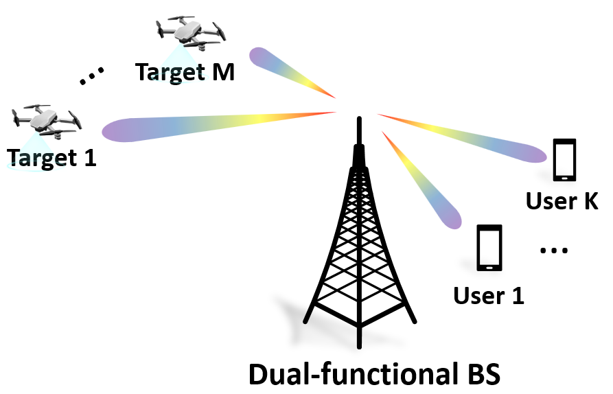
A DFRC BS is serving single-antenna communication users and sensing radar targets as shown in Fig. 1. The BS is equipped with a fully-digital uniform linear array (ULA) with transmit antennas. Without loss of generality, the space between the adjacent elements for both the transmit array is , where denotes the wavelength. The users and the targets are assumed to be sufficiently far from the BS, and thus the target can be viewed as points [6].
We assume baseband data streams transmitted from the BS for communication and sensing, denoted as , where streams are dedicated for communication, and all signals can be utilized for sensing. The transmitted signal satisfies independent complex Gaussian distribution such that . Then, the transmitted signal can be written as , where denotes the full digital transmit beamformer, which can be defined as,
| (1) |
The received signal at user can be represented as
| (2) |
where denotes the real channel between the BS and user , and denotes the additive white Gaussian noise (AWGN) at user . Accordingly, the received SINR at user can be derived as
| (3) |
with the received data rate at user obtained as
| (4) |
As for sensing, we denote as the direction of angle (DoA) of target . The communication and sensing data streams can be simultaneously employed for sensing the targets. Then, the beampattern gain at target can be written as
| (5) |
where is the steering vector towards angle , is the covariance matrix of the transmitted signal.
II-B CSI and Target Location Uncertainty Model
The real channel can be modeled as
| (6) |
where denotes the estimated channel, and is the CSI error following the bounded error model as [16]
| (7) |
Because we only focus on the angle of direction (AoD) of the point-like target under far-field assumption, consider the deviation of the target AoD, and the steering vector of target can be modeled as
| (8) |
where and denote the minimum and the maximum values of possible , respectively.
II-C Problem Formulation
Under the existence of CSI and AoD uncertainty in the ISAC system, we aim to propose a framework to maximize the weighted sum of worst-case user data rate and the beampattern gain, by optimizing the digital beamforming such that
| (9) | ||||
| s.t. | (9a) |
where is the weight allocated to communication function. Constraint (9a) denotes the power budget at the BS. The main challenges to solve this problem are i) the non-smooth objective function due to max-min problem; ii) the intractable CSI and angle uncertainty; iii) the non-convex expression of and as the objective function.
III Robust Beamforming Optimization
In this section, we provide the proposed solution for the robust beamforming design. Since constraint (9a) is already convex, we focus on dealing with the non-convex objective function. Specifically, (P1) can be separated to communication and sensing parts as
| (10) | ||||
| s.t. |
| (11) | ||||
| s.t. |
Then, we will discuss the solutions to (P1-a) and (P1-b) in section III.A and section III.B, respectively.
III-A Solving (P1-a) with S-Procedure
Focusing on communication, by introducing auxiliary variable , (P1-a) can be further transformed as
| (12) | ||||
| s.t. | (12a) | |||
where (12a) is equivalent to
| (13) | |||
| (14) | |||
| (15) |
where and are slack variables. The main challenge introduced by the communication measurement is to tackle the above three non-convex constraints.
Recalling (6), (13) can be rewritten as
| (16) |
where the quadratic expression with respect to variable makes the constraint non-convex. Thus, this problem can be solved iteratively by successive convex approximation (SCA) method. The lower bound of the left-hand-side can be approximated by its first Taylor expansion, and (16) can be further transformed as
| (17) |
where , and can be obtained by
| (18) | |||
| (19) | |||
| (20) |
where denotes the results obtained at the last iteration.
Next, the S-Procedure is employed to deal with the bounded CSI error model, and (17) is equivalent to
| (21) |
where , are slack variables.
As for (14), first we apply Schur complement to transform (14) as
| (22) |
where is stacked as
| (23) |
Then, (22) can be further equivalently transformed as [17]
| (24) |
where , are the slack variables.
To address (15), we first rewrite it as
| (25) |
where the two slack variables at the right-hand-side of the inequality are decoupled by rewriting it as a difference of convex function. We further linearly approximate its upper bound, and then (15) is obtained as
| (26) |
Based on the above derivations, problem (P1-a) can be reformulated as
| (27) | ||||
| s.t. |
III-B Solving (P1-b) with Convex Hull
Focusing on (P1-b), to make the sensing beampattern gain more tractable, (5) can be rewritten as
| (28) |
where . Because we only focus on sensing in this stage, temporarily ignoring communication metric and constant , problem (P1-b) can be reduced as
| (29) | ||||
where . To make it tractable, we construct a convex hull of as [18]
| (30) |
where is the weight, is the total number of samples, and is the -th sample. By focusing on the sum of beampattern gain in the objective function, and ignoring the constraints discussed in the last part, we have the following proposition.
Proposition 1: To maximize the the sum of minimization over the set is equivalent to that over , which can be represented as
| (31) |
Proof: The proof can be referred to [18].
Thus, problem (P1-b1) is equivalent to
| (32) | ||||
Then, we will optimize and in two layers.
In the outer layer, assuming is fixed, the reverse Hlder inequality can be applied as
| (33) |
where the equality holds if and only if . Together with , the that results in the worst case beampattern gain can be computed as
| (34) |
where denotes the optimal value obtained at the last iteration.
In the inner layer, with fixed , (P1-b2) can be reformulated as
| (35) | ||||
where . To solve this non-convex problem, SCA method can be utilized again to approximate the objective function by its first Taylor expansion as
| (36) |
Then with the approximation, (P1-b3) is transformed to be a simple convex problem. Because (P1-a2) about communication is unrelated to updating , we update beamforming matrix in the inner layer, by combining the communication part solving (P1-a2) in section III.A with sensing part solving the transformed (P1-b3) as
| (37) | |||
which is an semidefinite programming (SDP) problem that can be efficiently solved by the existing toolbox such as CVX.
III-C Overall Algorithm
Overall, problem (P2) can be solved by two layers, where is optimized in the outer layer, and is updated in the inner layer. The overall algorithm is summarized as Algorithm 1 and Algorithm 2.
The computational complexity of the proposed robust algorithm mainly depends on the complexity of optimizing in Algorithm 1 and updating in Algorithm 2. In the inner loop, solving problem (P2) contains variables of order , quadratic constraints and linear matrix inequality constraints with sizes and , respectively. Thus, the total computational complexity of solving problem (P2) is , where denotes the number of iterations of the inner loop, and denotes the accuracy of the SCA based method. In the outer loop, the main complexity depends on computing with (34), which is . Finally, the overall computational complexity of the proposed Algorithm 2 can be represented as , where is the number of iterations of the outer loop.
IV Numerical Results
In this section, we provide numerical simulations to evaluate the performance of our proposed robust beamforming algorithm for the ISAC system. We assume the BS is equipped with transmit antennas, serving users and sensing targets. The distances between the BS and the users are set as between 20 and 70 m. The estimated AoDs of the users and targets are and , respectively. The bound for CSI error is defined as , with coefficient . The range for target AoD uncertainty is denoted as . For simplicity, we assume that the angle uncertainty for each target is the same, i.e. .
The distance dependent path loss is dB, where denotes the distance, and is the path loss exponent. The noise powers are assumed to be dBm. To verify the effectiveness and performance improvement of our proposed robust algorithm, we have two baselines, i) non-robust: optimizing the transmit beamforming matrix with estimated user channels and target angles by SCA-based algorithm; ii) steering vector matching (SVM): aligning each column of the beamforming matrix with the array response vectors of the corresponding users and targets.
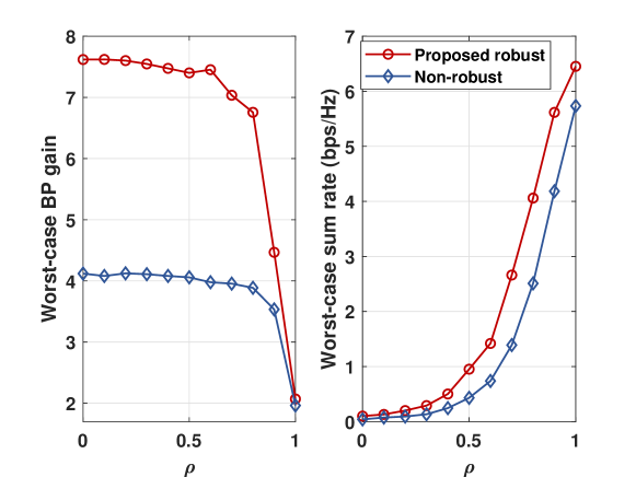
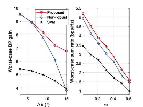
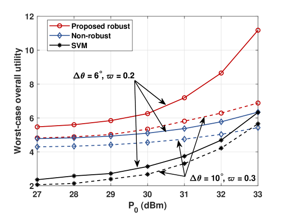
Fig. 2 shows the trade-off between communication and sensing performance with varying weighting factor . We set and for sensing performance analysis and and for communication. It can be observed that the proposed robust algorithm significantly outperforms non-robust optimization, especially on sensing performance. This is because the proposed algorithm directly optimizes the worst-case beampattern (BP) gain in terms of sensing. Also, the trend along illustrates the trade-off between the two functions. The worst-case sum rate increases rapidly, while the beampattern gain decreases with the rising , as higher weight is assigned to communication. This feature facilitates the design of weight allocation tailored to practical requirements.
Fig. 3 shows the effect of angle and CSI uncertainty on sensing and communication performance, respectively. The proposed robust algorithm achieves higher beampattern gain and sum rate compared to the two baselines. The worst-case beampattern gain decreases with larger angle error, reflecting a similar trend in communication performance. This is intuitive that large error in AoD and channel estimation will negatively impact beamforming design.
Fig. 4 illustrates the worst-case overall utility (weighted sum of sensing beampattern gain and communication data rate) versus the transmit power . The total utility increases fast as the power budget at the base station grows. We provide two sets of angle and CSI error parameters, i.e. and . The results indicate that the proposed robust algorithm performs better with more accurate estimation, which is consistent with the findings in Fig. 3.
V Conclusion
In conclusion, this paper introduced a dual-robust ISAC system considering imperfect CSI and uncertain target location. A two-layer iterative algorithm was proposed to address the joint sensing and communication optimization problem. Numerical results revealed that our algorithm enhanced robust performance and verified the trends in sensing and communication with varying weighting factor. Additionally, the convex hull-based worst-case sensing optimization exhibited greater potential compared to the S-Procedure-based worst-case communication optimization.
References
- [1] F. Liu, Y. Cui, C. Masouros, J. Xu, T. X. Han, Y. C. Eldar, and S. Buzzi, “Integrated sensing and communications: Toward dual-functional wireless networks for 6G and beyond,” IEEE J. Sel. Areas Commun., vol. 40, no. 6, pp. 1728–1767, Jun. 2022.
- [2] J. An, H. Li, D. W. K. Ng, and C. Yuen, “Fundamental detection probability vs. achievable rate tradeoff in integrated sensing and communication systems,” IEEE Trans. Wireless Commun., vol. 22, no. 12, pp. 9835–9853, Dec. 2023.
- [3] X. Shao, C. You, W. Ma, X. Chen, and R. Zhang, “Target sensing with intelligent reflecting surface: Architecture and performance,” IEEE J. Sel. Areas Commun., vol. 40, no. 7, pp. 2070–2084, Jul. 2022.
- [4] Z. Wang, Y. Liu, X. Mu, Z. Ding, and O. A. Dobre, “NOMA empowered integrated sensing and communication,” IEEE Commun. Lett., vol. 26, no. 3, pp. 677–681, Mar. 2022.
- [5] K. Meng, Q. Wu, J. Xu, W. Chen, Z. Feng, R. Schober, and A. L. Swindlehurst, “UAV-enabled integrated sensing and communication: Opportunities and challenges,” IEEE Wireless Communications, pp. 1–9, 2023.
- [6] F. Liu, C. Masouros, A. Li, H. Sun, and L. Hanzo, “MU-MIMO communications with mimo radar: From co-existence to joint transmission,” IEEE Trans. Wireless Commun., vol. 17, no. 4, pp. 2755–2770, Apr. 2018.
- [7] C. Qi, W. Ci, J. Zhang, and X. You, “Hybrid beamforming for millimeter wave MIMO integrated sensing and communications,” IEEE Commun. Lett., vol. 26, no. 5, pp. 1136–1140, MAy, 2022.
- [8] X. Wang, Z. Fei, J. A. Zhang, and J. Xu, “Partially-connected hybrid beamforming design for integrated sensing and communication systems,” IEEE Trans. Commun., vol. 70, no. 10, pp. 6648–6660, Oct. 2022.
- [9] Y. He, Y. Cai, H. Mao, and G. Yu, “Ris-assisted communication radar coexistence: Joint beamforming design and analysis,” IEEE J. Sel. Areas Commun., vol. 40, no. 7, pp. 2131–2145, Jul. 2022.
- [10] H. Luo, R. Liu, M. Li, Y. Liu, and Q. Liu, “Joint beamforming design for RIS-assisted integrated sensing and communication systems,” IEEE Trans. Veh. Technol., vol. 71, no. 12, pp. 13 393–13 397, Dec. 2022.
- [11] Y. Peng, S. Yang, W. Lyu, Y. Li, H. He, Z. Zhang, and C. Assi, “Mutual Information-Based Integrated Sensing and Communications: A WMMSE Framework,” arXiv e-prints, p. arXiv:2310.12686, Oct. 2023.
- [12] A. Bazzi and M. Chafii, “Robust Integrated Sensing and Communication Beamforming for Dual-functional Radar and Communications: Method and Insights,” arXiv e-prints, p. arXiv:2303.07652, Mar. 2023.
- [13] S. Wang, W. Dai, H. Wang, and G. Y. Li, “Robust Waveform Design for Integrated Sensing and Communication,” arXiv e-prints, p. arXiv:2311.00071, Oct. 2023.
- [14] Z. Ren, L. Qiu, J. Xu, and D. W. K. Ng, “Robust transmit beamforming for secure integrated sensing and communication,” IEEE Trans. Commun., vol. 71, no. 9, pp. 5549–5564, Sep. 2023.
- [15] M. Luan, B. Wang, Z. Chang, T. Hämäläinen, and F. Hu, “Robust beamforming design for RIS-aided integrated sensing and communication system,” IEEE Transactions on Intelligent Transportation Systems, vol. 24, no. 6, pp. 6227–6243, Jun. 2023.
- [16] Y. Xu, H. Xie, Q. Wu, C. Huang, and C. Yuen, “Robust max-min energy efficiency for RIS-aided hetnets with distortion noises,” IEEE Trans. Commun., vol. 70, no. 2, pp. 1457–1471, Feb. 2022.
- [17] G. Zhou, C. Pan, H. Ren, K. Wang, M. D. Renzo, and A. Nallanathan, “Robust beamforming design for intelligent reflecting surface aided MISO communication systems,” IEEE Wireless Commun. Lett., vol. 9, no. 10, pp. 1658–1662, Oct. 2020.
- [18] Z. Lin, M. Lin, J.-B. Wang, Y. Huang, and W.-P. Zhu, “Robust secure beamforming for 5G cellular networks coexisting with satellite networks,” IEEE J. Sel. Areas Commun., vol. 36, no. 4, pp. 932–945, Apr. 2018.