\AtAppendix

Barter Exchange with Shared Item Valuations

Juan Luque Department of Computer ScienceUniversity of MarylandCollege ParkMDUSA , Sharmila Duppala Department of Computer ScienceUniversity of MarylandCollege ParkMDUSA , John Dickerson Department of Computer ScienceUniversity of MarylandCollege ParkMDUSA and Aravind Srinivasan Department of Computer ScienceUniversity of MarylandCollege ParkMDUSA

Abstract.

In barter exchanges agents enter seeking to swap their items for other items on their wishlist. We consider a centralized barter exchange with a set of agents and items where each item has a positive value. The goal is to compute a (re)allocation of items maximizing the agents’ collective utility subject to each agent’s total received value being comparable to their total given value. Many such centralized barter exchanges exist and serve crucial roles; e.g., kidney exchange programs, which are often formulated as variants of directed cycle packing. We show finding a reallocation where each agent’s total given and total received values are equal is NP-hard. On the other hand, we develop a randomized algorithm that achieves optimal utility in expectation and where, i) for any agent, with probability 1 their received value is at least their given value minus $v^{*}$ where $v^{*}$ is said agent’s most valuable owned and wished-for item, and ii) each agent’s given and received values are equal in expectation.

Barter-Exchanges, Centralized exchanges, Community Markets

^†^†copyright: none^†^†price: ^†^†ccs: Theory of computation Rounding techniques^†^†ccs: Applied computing Electronic commerce

1. Introduction

Social media platforms have recently emerged into small scale business websites. For example, platforms like Facebook, Instagram, etc. allow its users to buy and sell goods via verified business accounts. With the proliferation of such community marketplaces, there are growing communities for buying, selling and exchanging (swapping) goods amongst its users. We consider applications, viewed as Barter Exchanges, which allow users to exchange board games, digital goods, or any physical items amongst themselves. For instance, the subreddit GameSwap¹¹1www.reddit.com/r/Gameswap (61,000 members) and Facebook group BoardgameExchange²²2https://www.facebook.com/groups/boardgameexchange (51,000 members) are communities where users enter with a list of owned video games and board games. The existence of this community is testament to the fact that although users could simply liquidate their goods and subsequently purchase the desired goods, it is often preferable to directly swap for desired items. Additionally, some online video games have fleshed out economies allowing for the trade of in-game items between players while selling items for real-world money is explicitly illegal e.g., Runescape³³3www.jagex.com/en-GB/terms/rules-of-runescape. In these applications, a centralized exchange would achieve greater utility, in collective exchanged value and convenience, as well as overcome legality obstacles.

A centralized barter exchange market provides a platform where agents can exchange items directly, without money/payments. Beyond the aforementioned applications, there exist a myriad of other markets facilitating the exchange of a wide variety of items, including books, children’s items, cryptocurrency, and human organs such as kidneys. There are both centralized and decentralized exchange markets for various items. HomeExchange⁴⁴4www.homeexchange.com and ReadItSwapIt⁵⁵5www.readitswapit.co.uk are decentralized marketplaces that facilitate pairwise exchanges by mutual agreement of vacation homes and books, respectively. Atomic cross chain swaps allow users to exchange currencies within or across various cryptocurrencies (e.g., Herlihy, 2018; Thyagarajan et al., 2022). Kidney exchange markets (see, e.g., Aziz et al., 2021; Abraham et al., 2007) and children’s items markets (e.g., Swap⁶⁶6www.swap.com) are examples of centralized exchanges facilitating swaps amongst incompatible patient-donor pairs and children items or services amongst parents. Finding optimal allocations is often NP-hard. As a result heuristic solutions have been explored extensively (Glorie et al., 2014; Plaut et al., 2016).

Currently, the aforementioned communities GameSwap and BoardGameExchange make swaps in a decentralized manner between pairs of agents, but finding such pairwise swaps is often inefficient and ineffective due to demanding a “double coincidence of wants” (Jevons, 1879). However, centralized multi-agent exchanges can help overcome such challenges by allowing each user to give and receive items from possibly different users. Moreover, the user’s goal is to swap a subset of their owned games for a subset of their desired games with comparable (or greater) value. Although an item’s value is subjective, a natural proxy is its re-sale price, which is easily obtained from marketplaces such as Ebay.

We consider a centralized exchange problem where each agent has a have-list and a wishlist of distinct (indivisible) items (e.g., physical games) and, more generally, each item has a value agreed upon by the participating agents (e.g., members of the GameSwap community). The goal is to find an allocation/exchange that (i) maximizes the collective utility of the allocation such that (ii) the total value of each agent’s items before and after the exchange is equal.⁷⁷7Equivalently, the total value of the items given is equal to the total value of the items received. We call this problem barter with shared valuations, $\mathsf{BarterSV}$ , and it is our subject of study. Notice that bipartite perfect matching is a special case of $\mathsf{BarterSV}$ where each agent has a single item in both its have-list and wishlist each and where all the items are have the same value. On the other hand, we show $\mathsf{BarterSV}$ is NP-Hard (Theorem 2).

In the following sections we formulate $\mathsf{BarterSV}$ as bipartite graph-matching problem with additional barter constraints. Our algorithm BarterDR is based on rounding the fractional allocation of the natural LP relaxation to get a feasible integral allocation. A direct application of existing rounding algorithms (like (Gandhi et al., 2006)) to $\mathsf{BarterSV}$ results in a worst-case where some agents give away all their items and receive none in exchange. This is wholly unacceptable for any deployed centralized exchange. In contrast, our main result ensures BarterDR allocations have reasonable net value for all agents; more precisely each agent gives and receives the same value in expectation and the absolute difference between given and received values is at most the value of their most valuable item (Theorem 1).

1.1. Problem formulation: $\mathsf{BarterSV}$

Suppose we are given a ground set of items $\mathcal{I}$ to be swapped, item values $\{v_{j}\in\mathbb{R}^{+}:j\in\mathcal{I}\}$ where $\mathbb{R}^{+}$ denotes the non-negative real numbers, and a community of agents $\mathcal{N}=[n]$ where $[n]$ denotes $\{1,2,\dots,n\}$ . Each agent $i$ possesses items $H_{i}\subseteq\mathcal{I}$ and has wishlist $W_{i}\subseteq\mathcal{I}$ . A valid allocation of these items involves agents swapping their items with other agents that desire said item. Let $w(i,i^{\prime},j)$ denote the utility gained when agent $i$ gives an item $j\in H_{i}\cap W_{i^{\prime}}$ to an agent $i^{\prime}$ . The goal of $\mathsf{BarterSV}$ is to find a valid allocation of maximum utility subject to no agent giving away more value than they received. Formally, any valid allocation is represented by the function $g:\mathcal{N}\times\mathcal{N}\times\mathcal{I}\rightarrow\{0,1\}$ such that $g(i,i^{\prime},j)=1$ if agent $i$ gives agent $i^{\prime}$ item $j$ and $g(i,i^{\prime},j)=0$ , otherwise. Additionally, each agent $i\in\mathcal{N}$ (i) receives only desired items, meaning $\sum_{i^{\prime}\in\mathcal{N}}g(i^{\prime},i,j)\leq 1$ if $j\in W_{i}$ , and $\sum_{i^{\prime}\in\mathcal{N}}g(i^{\prime},i,j)\leq 0$ otherwise; and (ii) gives away only items they possess, thus $\sum_{i^{\prime}\in\mathcal{N}}g(i,i^{\prime},j)\leq 1$ if $j\in H_{i}$ , and $\sum_{i^{\prime}\in\mathcal{N}}g(i,i^{\prime},j)\leq 0$ otherwise. We begin by defining a special variant of a graph matching problem called Value-balanced Matching (VBM).

Definition 0.

Value-balanced Matching (VBM) Suppose there is bipartite graph $G=(L,R,E)$ with vertex values $v_{a}>0$ $\forall a\in L\cup R$ . Let each edge $e\in E$ have weight $w_{e}\in\mathbb{R}$ , $L=\dot{\bigcup}_{i}L_{i}$ , and $R=\dot{\bigcup}_{i}R_{i}$ . For a given matching $M\subseteq E$ , let ${V_{i}}^{(L)}=\sum_{\ell:(\ell,r)\in M,\ell\in L_{i}}v_{\ell}$ and ${V_{i}}^{(R)}=\sum_{r:(\ell,r)\in M,r\in R_{i}}v_{r}$ , where $\dot{\bigcup}$ denotes disjoint union. The goal of VBM is to find $M$ of maximum weight subject to, for each $i$ , the value of items matched in $L_{i}$ and $R_{i}$ are equal i.e., ${V_{i}}^{(R)}={V_{i}}^{(L)}$ .

Refer to caption — Figure 1. A VBM instance for a $\mathsf{BarterSV}$ instance with $\mathcal{N}=\{1,2\}$ , $\mathcal{I}=\{a,b,c,d\}$ , $H_{1}=\{a,b\}$ , $W_{1}=\{c,d\}$ , $H_{2}=\{c\}$ , $W_{2}=\{a,d\}$ , $H_{3}=\{d\}$ , $W_{3}=\{b,c\}$ , $v_{a}=100$ , $v_{b}=v_{c}=v_{d}=1$ , and $w_{e}=1$ for all $e\in E$

Lemma 1.0.

For any instance $\mathcal{B}$ of $\mathsf{BarterSV}$ , there exists a corresponding instance $\mathcal{G}$ of VBM such that the utility of an optimal allocation in the instance $\mathcal{B}$ is equal to the optimal weight matching in the corresponding instance $\mathcal{G}$ and vice-versa.

Proof.

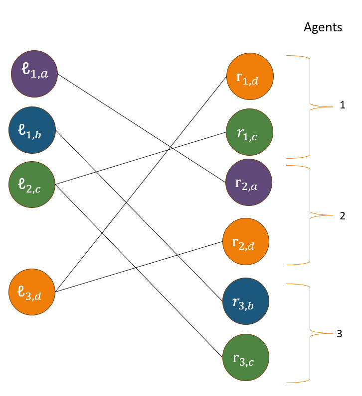
Given a $\mathsf{BarterSV}$ instance $\mathcal{B}$ given by $(\mathcal{N},\mathcal{I},\{v_{j}\}_{j\in\mathcal{I}},(H_{i},W_{i})_{i\in[n]},w)$ we can reduce it to a corresponding instance $\mathcal{G}$ of VBM via the construction of an appropriate bipartite graph with vertex values. For each agent $i\in\mathcal{N}$ , build the vertex sets $L_{i}:=\{\ell_{ij}:j\in H_{i}\}$ and $R_{i}:=\{r_{ij}:j\in W_{i}\}$ . Then the bipartite graph of interest has vertex sets $L=\dot{\bigcup}_{i\in[n]}L_{i}$ and $R=\dot{\bigcup}_{i\in[n]}R_{i}$ , as well as edge set $E:=\{(\ell_{ij},r_{i^{\prime}j}):j\in H_{i}\cap W_{i^{\prime}}\wedge i,i^{\prime}\in\mathcal{I}\}$ . For each edge $e=(\ell_{ij},r_{i^{\prime}j})$ , the weight of $e$ is given by $w_{e}:=w(i,i^{\prime},j)$ . Each vertex $\ell_{ij}$ and $r_{i^{\prime}j}$ has vertex values $v_{j}$ i.e., $v_{\ell_{ij}},v_{r_{i^{\prime}j}}:=v_{j}$ . Notice that the edges in $E$ represent vertices belonging the same item, hence they have identical values. Refer to Figure 1 for an example constructing a VBM instance.

Suppose we are given any feasible allocation $g$ for an instance $\mathcal{B}$ of $\mathsf{BarterSV}$ with utility of $D$ , then we can say construct a feasible matching $M$ corresponding to instance $\mathcal{G}$ of weight $D$ . We construct the matching as follows. For any $i,i^{\prime}\in\mathcal{N}$ and $j\in H_{i}\cap W_{i^{\prime}}$ , if $g(i,i^{\prime},j)=1$ , then add the edge $e=(\ell_{ij},r_{i^{\prime}j})$ to $M$ . The total weight of the matching is given by $\sum_{e\in M}w_{e}=\sum_{(\ell_{ij},r_{i^{\prime}j})\in M}w(i,i^{\prime},j)=D$ . It remains to show that $M$ is indeed a value-balanced matching. We begin by showing that $M$ is a feasible matching to the VBM problem. Since $g$ is a valid allocation to $\mathcal{B}$ , we can say that for any agent $i\in\mathcal{N}$ , the value of the items received is equal to the value of the items given away i.e., $\sum_{j\in H_{i}}\sum_{i^{\prime}\in\mathcal{N}}g(i,i^{\prime},j)=\sum_{j\in W_{i}}\sum_{i^{\prime}\in\mathcal{N}}g(i^{\prime},i,j)$ . This implies that for each $g(i,i^{\prime},j)=1$ , we have $(l_{ij},r_{i^{\prime}j})\in M$ , therefore, $V_{i}^{(L)}=V_{i}^{(R)}$ . Thus, $M$ is a feasible VBM matching.

To prove the other direction we begin by assuming that $M$ is a feasible matching to $\mathcal{G}$ of weight $D$ . Given $M$ , we can construct a feasible allocation $g$ by assigning $g(i,i^{\prime},j)=1$ if the edge $(\ell_{ij},r_{i^{\prime}j})\in M$ , and $g(i,i^{\prime},j)=0$ otherwise. Notice that $g$ is a valid allocation; for any agent $i\in\mathcal{N}$ , the value of items received is equal to the value of the items given away. This is because $M$ is a feasible matching to VBM, meaning for any $i\in[n]$ , $V_{i}^{(L)}=V_{i}^{(R)}$ implying that $\sum_{i^{\prime}\in\mathcal{N}}\sum_{j\in H_{i}\cap W_{i^{\prime}}}g(i,i^{\prime},j)=\sum_{i^{\prime}\in\mathcal{N}}\sum_{j\in W_{i}\cap H_{i^{\prime}}}g(i^{\prime},i,j)$ . The utility of allocation is given by $\sum_{i^{\prime},i\in N}\sum_{j\in H_{i}\cap W_{i^{\prime}}}w(i,i^{\prime},j)=\sum_{e=(\ell_{ij},r_{i^{\prime}j})\in M}w_{e}=D.$ This completes our proof. ∎

Corollary 0.

$\mathsf{BarterSV}$ is equivalent to VBM.

The proof of the corollary directly follows from Lemma 2.

1.2. LP formulation of VBM

Any feasible matching $M$ in $(L,R,E)$ such that for each $e\in E$ , $x_{e}=1$ if $e\in M$ and $x_{e}=0$ otherwise is feasible in the following Integer Program (IP);


(1a)	$\displaystyle\max\quad$	$\displaystyle\sum_{e\in E}w_{e}x_{e}$
(1b)	subj. to	$\displaystyle x(\ell_{ij})\leq 1,$	$\displaystyle i\in[n],\ell_{ij}\in L_{i}$
(1c)		$\displaystyle x(r_{ij})\leq 1,$	$\displaystyle i\in[n],r_{ij}\in R_{i}$
(1d)		$\displaystyle\sum_{a\in L_{i}}x(a)v_{a}=\sum_{b\in R_{i}}x(b)v_{b},$	$\displaystyle i\in[n]$
(1e)		$\displaystyle x_{e}\in\{0,1\},$	$\displaystyle e=(\ell_{ij},r_{i^{\prime}j})\in E$	.

For $a\in L\cup R$ , we denote $x(a):=\sum_{e\in N(a)}x_{e}$ where $N(a)$ denotes the open neighborhood of $a$ i.e., $N(a):=\{(a,b)\in E:b\in L\cup R\}$ . Thus we can say that if an edge $e=(\ell_{ij},r_{i^{\prime}j})\in M$ says agent $i$ gives item $j$ to agent $i^{\prime}$ in the corresponding $\mathsf{BarterSV}$ instance.

Lemma 1.0.

IP (1) is equivalent to $\mathsf{BarterSV}$ . Moreover, the objective of $\mathsf{BarterSV\text{-}LP}$ is an upper bound on the objective of IP (1).

Proof.

IP (1) is clearly equivalent to VBM and VBM is equivalent to $\mathsf{BarterSV}$ , per Corollary 3. The objective of IP 1, $\sum_{e\in E}w_{e}x_{e}$ is the allocation’s utility. By relaxing (1e) to $x_{e}\geq 0$ for $e\in E$ we arrive at the natural LP relaxation of $\mathsf{BarterSV}$ , namely $\mathsf{BarterSV\text{-}LP}$ , which can only have a greater optimal objective value. ∎

We conclude this section by a simple note. For each $e=(\ell_{ij},r_{i^{\prime}j})\in E$ we may set $w_{e}=v_{j}$ and recover the objective of maximizing the collective value received by all agents. Nevertheless, our results hold even if $w_{e}$ is set arbitrarily. For example, the algorithm designer could place greater value on certain item transactions, or they may maximize the sheer number of items received by uniformly setting $w_{e}=1$ .

2. Preliminaries: GKPS dependent rounding

Our results build on the dependent rounding algorithm due to (Gandhi et al., 2006), henceforth referred to as GKPS-DR. GKPS-DR is an algorithm that takes $\{x_{e}\}\in[0,1]^{|E|}$ defined over the edge set $E$ of a biparite graph $(L,R,E)$ and outputs $\{X_{e}\}\in\{0,1\}^{|E|}$ . In each iteration GKPS-DR considers the graph of floating edges (those edges $e$ with $0<x_{e}<1$ ) and selects a maximal path or cycle $P\subseteq E$ on floating edges. The edges of $P$ are decomposed into alternate matchings $M_{1}$ and $M_{2}$ and rounded in the following way. Fix $\alpha^{\text{GKPS}}=\min\left\{\gamma>0:\left(\bigvee_{e\in M_{1}}x_{e}+\gamma=1\right)\vee\left(\bigvee_{e\in M_{2}}x_{e}-\gamma=0\right)\right\}$ , and $\beta^{\text{GKPS}}=\min\left\{\gamma>0:\left(\bigvee_{e\in M_{2}}x_{e}+\gamma=1\right)\vee\left(\bigvee_{e\in M_{1}}x_{e}-\gamma=0\right)\right\}$ . Thus, each $x_{e}$ is updated to $x_{e}^{\prime}$ according to one of the following disjoint events: with probability $\frac{\beta^{\text{GKPS}}}{\alpha^{\text{GKPS}}+\beta^{\text{GKPS}}}$

x_{e}^{\prime}=\begin{cases}x_{e}+\alpha,&e\in M_{1}\\ x_{e}-\alpha,&e\in M_{2}\end{cases};\quad\text{else,}\quad x_{e}^{\prime}=\begin{cases}x_{e}-\beta,&e\in M_{1}\\ x_{e}+\beta,&e\in M_{2}.\end{cases}

The selection of $\alpha$ and $\beta$ ensures at least one edge is rounded to $0$ or $1$ in every iteration. GKPS-DR guarantees (P1) marginal, (P2) degree preservation, and (P3) negative correlation properties:

(P1)

$\forall e\in E$ , $\Pr(X_{e}=1)=x_{e}$ .
(P2)

$\forall a\in L\cup R$ and with probability 1, $X(a)\in\{\lfloor x(a)\rfloor,\lceil x(a)\rceil\}$ .
(P3)

$\forall a\in L\cup R,\;\forall S\subseteq N(a),\;\forall c\in\{0,1\}$ , $\Pr\left(\bigwedge_{s\in S}X_{s}=c\right)\leq\prod_{s\in S}\Pr\left(X_{s}=c\right)$ .

Remark 1.

When GKPS-DR rounds a path between vertices $a$ and $b$ , the signs of the changes to $x(a)$ and $x(b)$ are equal if and only if $a$ and $b$ belong to different graph sides.

3. Related work

Centralized barter exchanges have been studied by several others in the context of kidney-exchanges (Abraham et al., 2007; Ashlagi et al., 2018; Aziz et al., 2021). $\mathsf{BarterSV}$ generalizes a well-studied kidney-exchange problem in the following way. The Kidney Exchange Problem (KEP) is often formulated as directed cycle packing in compatibility patient-donor graphs (Abraham et al., 2007) where each node in the graph corresponds to a patient-donor pair and directed edges between nodes indicate compatibility. Abraham et al. (2007); Biró et al. (2009) observed this problem reduces to bipartite perfect matching, which is solvable in polynomial-time. We show $\mathsf{BarterSV}$ is NP-Hard and thus resort to providing a randomized algorithm with approximate guarantees on the agents’ net values via LP relaxation followed by dependent rounding.

There has been extensive work on developing dependent rounding techniques, that round the fractional solution in some correlated way to satisfy both the hard constraints and ensure some negative dependence amongst rounded variables that can result in concentration inequalities. For instance, the hard constraints might arise from an underlying combinatorial object such as a packing (Brubach et al., 2017), spanning tree (Chekuri et al., 2010), or matching (Gandhi et al., 2006) that needs to be produced. In our case, the rounded variables must satisfy both matching (1b), (1c), and barter constraints (1d) (i.e., each agent gives the items of same total value as it received). Gandhi et al. (2006) developed a rounding scheme where the rounded variables satisfy the matching constraints along with other useful properties. Therefore, we adapt their rounding scheme (to satisfy matching constraints) followed by a careful rounding scheme that results in rounded variables satisfying the barter constraints.

Centralized barter exchanges are well-studied under various barter settings. For instance, Abraham et al. (2007) showed that the bounded length edge-weighted directed cycle packing is NP-Hard which led to several heuristic based methods to solve these hard problems, e.g., by using techniques of operations research (Constantino et al., 2013; Glorie et al., 2014; Plaut et al., 2016; Carvalho et al., 2021), AI/ML modeling (McElfresh et al., 2020; Noothigattu et al., 2020). Recently several works focused on the fairness in barter exchange problems (Abbassi et al., 2013; Fang et al., 2015; Klimentova et al., 2021; Farnadi et al., 2021). Our work adds to the growing body of research in theory and heuristics surrounding ubiquitous barter exchange markets.

4. Outline of our contributions and the paper

Firstly, we introduce the $\mathsf{BarterSV}$ problem, a natural generalization of edge-weighted directed cycle packing and show that it is NP-Hard to solve the problem exactly. Our main contribution is a randomized dependent rounding algorithm BarterDR with provable guarantees on the quality of the allocation. The following definitions help present our results. Suppose we are given an integral allocation $\{X_{e}\}\in\{0,1\}^{|E|}$ , we define the net value loss of each agent $i$ (i.e., the violation in the barter constraint (1d)):

(2)

D_{i}:=\sum_{b\in L_{i}}v_{b}X(b)-\sum_{a\in R_{i}}v_{a}X(a).

Our main contribution is a rounding algorithm BarterDR that satisfies both matching ((1b) and (1c)) and barter constraints ((1d)) as desired in multi-agent exchanges. Recall that the rounding algorithm GKPS-DR (indeed a pre-processing step of BarterDR) rounds the fractional matching to an integral solution enjoying the properties mentioned in Section 2. The main challenge in our problem is satisfying the barter constraint. Here, a direct application of GKPS-DR alone can result in a worst case violation of $\sum_{a\in L_{i}}v_{a}$ on $D_{i}$ , corresponding to the agent losing all their items and gaining none (see the example in the Appendix). However, our algorithm BarterDR rounds much more carefully to ensure, for each agent $i$ , $D_{i}$ is at most $v_{i}^{*}:=\max_{a\in L_{i}\cup R_{i}}v_{a}$ , i.e., the most valuable item in $H_{i}\cup W_{i}$ . The two following theorems provide lower and upper bounds on tractable $D_{i}$ (i.e., (2)) guarantees for $\mathsf{BarterSV}$ . BarterDR on a bipartite graph $(L,R,E)$ is worst-case time $\mathcal{O}((|L|+|R|)(|L|+|R|+|E|))$ where $L,R=\mathcal{O}(|\mathcal{I}|n)$ . We view Theorem 1 as our main result.

Theorem 1.

Given a $\mathsf{BarterSV}$ instance, BarterDR is an efficient randomized algorithm achieving an allocation with optimal utility in expectation and where, for all agents $i$ , $D_{i}<v_{i}^{*}$ with probability $1$ and $\mathbb{E}[D_{i}]=0$ .

Theorem 2.

Deciding whether a $\mathsf{BarterSV}$ instance has a non-empty valid allocation with $D_{i}=0$ for all agents $i$ is NP-hard, even if all item values are integers.

Owing to its similarities to GKPS-DR, BarterDR enjoys similar useful properties:

Theorem 3.

BarterDR rounds $\{x_{e}\}\in[0,1]^{|E|}$ in the feasible region of $\mathsf{BarterSV\text{-}LP}$ into $\{X_{e}\}\in\{0,1\}^{|E|}$ while satisfying (P1), (P2), and (P3).

Outline of the paper

In Section 5 we describe BarterDR (Algorithm 1), our randomized algorithm for $\mathsf{BarterSV}$ , and its subroutines FindCCC and CCWalk in detail. Next, we give proofs and proof sketches for Theorems 1 and 3.

5. BarterDR: dependent rounding algorithm for $\mathsf{BarterSV}$

Notation

BarterDR is a rounding algorithm that proceeds in multiple iterations, therefore we use a superscript $r$ to denote the value of a variable at the beginning of iteration $r$ . An edge $e\in E$ is said to be floating if $x_{e}^{r}\in(0,1)$ . Analogously, let $E^{r}:=\{e\in E:x_{e}^{r}\in(0,1)\}$ , $a\in L\cup R$ is said to be a floating vertex if $x^{r}(a):=\sum_{e\in N(a)}x_{e}^{r}\not\in\mathbb{Z}$ and the sets of floating vertices are $L^{r}:=\{a\in L:x^{r}(a)\not\in\mathbb{Z}\}$ and $R^{r}:=\{a\in R:x^{r}(a)\not\in\mathbb{Z}\}$ . $L(E^{r})=\{a\in L\mid\exists(a,b)\in E^{r}\wedge a\in L\}$ . $R(E^{r})$ is defined similarly. $G^{r}:=(L(E^{r}),R(E^{r}),E^{r})$ . $K^{r}(a)$ denotes the connected component in $G^{r}$ containing vertex $a$ . Define $\kappa(i):=\{a:a\in L_{i}\cup R_{i}\}$ , for each $i\in[n]$ , to be the set of participating vertices in each barter constraint. We say two vertices $a,b\in L\cup R$ are partners if there exists $i\in[n]$ such that $a,b\in\kappa(i)$ and $a\neq b$ . Note if $a$ and $b$ are partners, then they are distinct vertices corresponding to items (owned or desired) of some common agent $i$ . In iteration $r$ , a vertex $a\in\kappa(i)$ is said to be partnerless if $\kappa(i)\cap(L^{r}\cup R^{r})=\{a\}$ ; i.e., $a$ is the only floating vertex in $\kappa(i)$ . We use the shorthand $a\sim b$ to denote $a$ and $b$ are partners. Edges and vertices not floating are said to be settled: once an edge $e$ (vertex $a$ ) is settled BarterDR will not modify $x_{e}$ ( $x(a)$ ). For vertices $a$ and $b$ , $a\leadsto b$ denotes a simple path from $a$ to $b$ . Define $D_{i}^{r}$ to be $D_{i}$ , as defined in (2), but with variables $\{x_{e}^{r}\}$ instead of $\{X_{e}\}$ . The fractional degree of $a\in L\cup R$ refers to $x^{r}(a)$ .

Once an edge is settled, its value does not change. In the each iteration BarterDR looks exclusively at the floating edges $E^{r}$ and the graph induced by them. Namely, $G^{r}:=(L(E^{r}),R(E^{r}),E^{r})$ where $L(E^{r}):=\{a\in L:\exists e\in E^{r},\;e\in N(a)\}$ and $R(E^{r})$ is defined analogously. In each iteration, at least one edge or vertex becomes settled, i.e., $|E^{r}|+|L^{r}|+|R^{r}|>|E^{r+1}|+|L^{r+1}|+|R^{r+1}|$ . Therefore BarterDR terminates in iteration $T$ where $|E^{T}|=0$ and $T\leq|L|+|R|+|E|$ .

Algorithm and analysis outline.

BarterDR begins by making $G$ acyclic via the pre-processing step in Section 5.1. Next, BarterDR proceeds as follows. While there are floating edges find an appropriate sequence of paths $\mathcal{P}$ constituting a CCC or CCW (defined in Section 5.2). The strategy for judiciously rounding $\mathcal{P}$ is fleshed out in Section 5.3. Finally, Section 5.4 concludes with proofs for Theorems 1 and 3.

5.1. Pre-processing: remove cycles in $G$

The pre-processing step consists of finding a cycle $C$ via depth-first search in the graph of floating edges and rounding $C$ via GKPS-DR until there are no more cycles. Let $\{x_{e}^{0}\}_{e\in E}$ denote the LP solution and $\{x^{1}_{e}\}_{e\in E}$ denote the output of the pre-processing step. BarterDR begins on $\{x^{1}_{e}\}_{e\in E}$ .

GKPS-DR on cycles never changes fractional degrees, i.e., $\forall a\in L\cup R,\;x^{0}(a)=x^{1}(a)$ . Lemma 3 is used to construct CCC’s and CCW’s, and it is the raison d’être for the pre-processing step.

Lemma 5.0.

The pre-processing step is efficient and gives $D_{i}^{1}=0$ for all agents $i$ with probability $1$ .

Proof.

The pre-processing step runs GKPS-DR on $G$ until no cycles remain. GKPS-DR on a cycle guarantees that at the end of each iteration the fractional vertex degrees remain unchanged. Moreover, the full GKPS algorithm takes time $O(|E|\cdot(||E|+|V|))$ , bounding the pre-processing step’s runtime which can be seen as GKPS with an early stoppage condition. ∎

Lemma 5.0.

Let $\{x_{e}\}\in(0,1)^{|E|}$ be a vector of floating edges over a bipartite graph $(U,V,E)$ . Then the number of floating vertices in $(U,V,E)$ is not 1.

Proof.

Let $u$ be the sole floating vertex, i.e., $x(u)\not\in\mathbb{Z}$ , and, without loss of generality, let $u\in U$ . For $S\subseteq U\cup V$ , let $d(S):=\sum_{s\in S}x_{s}$ . Then $d(U-\{u\})+x_{u}=d(U)=\sum_{e\in E}x_{e}=d(V)$ . But $u$ being the only floating vertex implies $d(U-\{u\})+x(u)\not\in\mathbb{Z}$ and $d(V)\in\mathbb{Z}$ . ∎

Lemma 5.0.

Each connected component of $G^{1}$ has at least $2$ floating vertices.

Proof.

Fix an arbitrary connected component $K$ of $G^{1}$ . If $K$ has 0 floating vertices, then each vertex has degree at least two because $\forall e\in E^{r},x_{e}^{r}\in(0,1)$ . This implies the existence of a cycle in $K$ , but this cannot happen as the pre-processing step eliminates all cycles. Applying Lemma 2 to $K$ , the only remaining possibility is that $G^{1}$ has at least two floating vertices. ∎

5.2. Construction of CCC’s and CCW’s via FindCCC

This section introduces CCC’s and CCW’s. The definition of these structures facilitates rounding edges while respecting the barter constraints each iteration. The subroutines for constructing CCC’s and CCW’s, FindCCC and CCWalk, are described in Algorithms 2 and 3. The correctness of these subroutines, and thus the existence of CCC’s and CCW’s, follows from Lemma 5.

Definition 0.

A connected component cycle (CCC) is a sequence of $q\geq 1$ paths $\mathcal{P}=\langle s_{1}\leadsto t_{1},\dots,s_{q}\leadsto t_{q}\rangle$ such that, letting $V(\mathcal{P})=\bigcup_{i\in[q]}\{s_{i},t_{i}\}$ be the paths’ endpoint vertices,

(1)

$\forall i\in[q]$ , $t_{i}\sim s_{i+1}$ (taking $s_{q+1}\equiv s_{1}$ ),
(2)

$\forall a\in V(\mathcal{P})$ , $|V(\mathcal{P})\cap\kappa(a)|=2$ ,
(3)

$\forall i\in[q]$ , $s_{i}\leadsto t_{i}$ belongs to a unique connected component, and
(4)

$\forall i\in[q]$ , $s_{i}$ and $t_{i}$ are floating vertices.

Instead, we have a connected component walk (CCW) if criteria 3) and 4) are met but 1) and 2) are relaxed to: 1) $\forall i\in[q-1]$ , $t_{i}\sim s_{i+1}$ and $s_{1}$ and $t_{q}$ are partnerless; and 2) $\forall a\in V(\mathcal{P})-\{s_{1},t_{q}\},|V(\mathcal{P})\cap\kappa(a)|=2$ .

Recall that a rounding iteration $r$ is fixed so whether a vertex is floating or partnerless is well-defined. When $\mathcal{P}$ is rounded the set of vertices whose fractional degrees change is precisely $V(\mathcal{P})$ . Requirements 1 and 2 of a CCC say $t_{i}$ and $s_{i+1}$ are partners and they do not have any other partner vertices in $V(\mathcal{P})$ . Comparably, for CCW’s these requirements imply the same for all vertices but the “first” and “last,” which are partnerless. Therefore, for CCC’s and CCW’s the vertices in $V(\mathcal{P})$ respectively appear in $q$ and $q+1$ distinct barter constraints. The requirements in the definitions of CCC and CCW come in handy during the analysis because: each path belongs to a different connected component hence they are vertex and edge disjoint; if a barter constraint has exactly two vertices in $V(\mathcal{P})$ then these vertices’ fractional degree changes can be made to cancel each other out in the barter constraint; and floating vertices ensure paths can be rounded in a manner analogous to GKPS-DR. For comparison, GKPS-DR also needed paths with floating endpoints, but maximal paths always have such endpoints whereas the paths of $\mathcal{P}$ need not be maximal. Consequently, the requirement that paths of $\mathcal{P}$ have floating endpoints must be imposed.

Input:

\{x_{e}^{1}\}\in[0,1]^{|E|}

, corresponding to

G^{1}=(L(E^{1}),R(E^{1}),E^{1})

; i.e., the output of the pre-processing described in Section 5.1

r\leftarrow 1

2 while $E^{r}\neq\emptyset$ do

\mathcal{P}\leftarrow

CCC or CCW returned by FindCCC in

G^{r}

4 Round

\mathcal{P}

as described in Section 5.3 yielding

G^{r+1}

and

\{x_{e}^{r+1}\}

r\leftarrow r+1

7 end while

return $\{x_{e}^{r}\}\in\{0,1\}^{|E|}$

Algorithm 1 BarterDR

Input:

G^{r}=(L(E^{r}),R(E^{r}),E^{r})

Output: CCC or CCW

\langle s_{i}\leadsto t_{i}\rangle_{i\in[q]}

s_{1},t_{1}\leftarrow

distinct floating vertices in some connected component

C

G_{r}

(O_{1},\sigma_{1})\leftarrow

\text{{CCWalk}}(t_{1})

3 if $\sigma_{1}=$ ”CCC” then

4 return $O_{1}$

(O_{2},\sigma_{2})\leftarrow

\text{{CCWalk}}(s_{1})

6 if $\sigma_{2}=$ ”CCC” then

7 return $O_{2}$

8 Let

O_{1}=(t_{1},s_{2},t_{2},\dots,s_{q},t_{q})

and

O_{2}=(t^{\prime}_{1},s^{\prime}_{2},t^{\prime}_{2},\dots,s^{\prime}_{q^{\prime}},t^{\prime}_{q^{\prime}})

9 If

O_{1}

and

O_{2}

“cross,” resolve

O_{1}

and

O_{2}

into a CCC and return it; see Section 5.2

return $\left<t^{\prime}_{q^{\prime}}\leadsto s^{\prime}_{q^{\prime}},t^{\prime}_{q^{\prime}-1},s^{\prime}_{q^{\prime}-1},\dots,s^{\prime}_{2}\leadsto t^{\prime}_{2},t^{\prime}_{1}\leadsto t_{1},s_{2}\leadsto t_{2},\dots,s_{q}\leadsto t_{q}\right>$

// CCW

Algorithm 2 FindCCC

Input:

G^{r}=(L(E^{r}),R(E^{r}),E^{r})

, the walk’s starting vertex

a

Output: A CCC or half of a CCW and a string indicating whether a CCC was returned

V\leftarrow(t_{1})

, letting

t_{1}:=a

// ordered list of path endpoints

S\leftarrow\{C_{1}\}

where

C_{1}=K^{r}(a)

S

is the set of seen CC’s

i\leftarrow 2

2 while True do

3 if $t_{i-1}$ is partnerless then

return $(V,\text{"CCW"})$

// Return half of a CCW

s_{i}\leftarrow

partner of

t_{i-1}

C_{i}\leftarrow

connected component containing

s_{i}

7 if $C_{i}\in S$ then //

C_{i}

was previously visited

C_{i}=C_{k}

for some

k<i

so let

s_{k}^{\prime}:=s_{i}

9 return $(\left<s^{\prime}_{k}\leadsto t_{k},\dots,s_{i-1}\leadsto t_{i-1}\right>,\text{"CCC"})$

t_{i}\leftarrow

floating vertex in

C_{i}

distinct from

s_{i}

V\leftarrow V\oplus(s_{i})

, where

\oplus

denotes sequence concatenation

12 if $\exists b\in V,\;b\sim t_{i}$ then //

t_{i}

already has a partner in

V

13 It must be that

b

already had a partner

c\in V

. WLOG,

b=t_{k-1}

and

c=s_{k}

, some

k\leq i

14 return $(\left<s_{k}\leadsto t_{k},\dots,s_{i}\leadsto t_{i}\right>,\text{"CCC"})$

V\leftarrow V\oplus(t_{i})

i\leftarrow i+1

S\leftarrow S\cup\{C_{i}\}

17 end while

Algorithm 3

\text{{CCWalk}}(a)

Uncrossing the half-CCWs.

We define what we mean by ”crossing” half-CCW’s in FindCCC Algorithm 2 and how to resolve this into a CCC. Using $O_{1}$ and $O_{2}$ build $\bar{V}:=\left<s_{q}^{\prime},t_{q-1}^{\prime},\dots,s_{2}^{\prime},t_{1}^{\prime},t_{1},s_{2},\dots,s_{q}\right>$ . $\bar{V}$ can be seen as the sequence of path endpoints (i.e., $V$ in CCWalk) resulting from a run of $\text{{CCWalk}}(s_{q}^{\prime})$ , which possibly did not stop when it should have returned a CCC. By the half-CCW’s ”crossing” we mean that in some iteration of the while-loop of CCWalk either a connected component is revisited or $t_{i}$ was partners with a vertex previously visited. But these cases are precisely Algorithms 3 and 3 from CCWalk where a CCC is resolved and returned.

Lemma 5.0.

If $G^{r}$ has no cycles, FindCCC efficiently returns a CCC or CCW.

Proof of Lemma 5.

$G^{r}$ for $r\geq 1$ is guaranteed to be acyclic by the pre-processing step. Recall, this acyclic property is used by Lemma 3 to guarantee each CC has at least two floating vertices. This ensures Algorithm 3 of FindCCC is well defined.

Let $V_{r}$ be the sequence of vertices $V$ at the beginning of iteration $r$ , and let $V_{r}-a$ denote $V_{r}$ without some vertex $a$ . Like in CCWalk, “ $\oplus$ ” denotes sequence concatenation. Let $a_{r}$ and $z_{r}$ be the first and last vertices of $V_{r}$ ; note $a_{r}$ does not change over iterations. We prove the correctness of CCWalk with the aid of the following loop invariants maintained at the beginning of each iteration $r$ of the while-loop.

(I1)

$z_{r}$ has no partners in $V_{r}$ .
(I2)

$\forall b\in V_{r}-z_{r}$ , $b$ has exactly one partner in $V_{r}$ .
(I3)

$a_{r}$ is the only vertex from $V_{r}$ in $K(a_{r})$ .
(I4)

$\forall b\in V_{r}-a_{r}$ , there are exactly two vertices from $V_{r}$ contained in $K(b)$ .

Proceed by induction. When $r=1$ , $V_{r}=\left<a\right>$ so $a_{r}=a=z_{r}$ so all invariants are (vacuously) true. Let $P(k)$ be the predicate saying all invariants hold at the beginning of iteration $k\geq 1$ . We assume $P(k)$ and show $P(k+1)$ .

If there is an iteration $k+1$ , then CCWalk did not return during iteration $k$ and must have added $\left<s_{k},t_{k}\right>$ to $V_{k}=\left<t_{1},s_{2},t_{2},\dots,s_{k-1},t_{k-1}\right>$ . If $z_{k+1}=t_{k}$ had a partner in $V_{k}\oplus\left<s_{k}\right>$ then iteration $k$ would have been the last as a CCC would have been returned. Therefore (I1) holds at the beginning of iteration $k+1$ .

By $P(k)$ , $\forall b\in V_{k}-t_{k-1}$ , $b$ has exactly one partner in $V_{k}$ and $t_{k-1}$ has zero partners in $V_{k}$ . By construction $s_{k}$ is selected to be the partner of $t_{k-1}$ so now $t_{k-1}$ and $s_{k}$ have exactly one partner each in $V_{k+1}$ . Therefore (I2) holds at the beginning of iteration $k+1$ .

If $V_{k+1}$ were to not meet (I3) then it must mean that either $s_{k}\in K(a_{k})$ or $t_{k}\in K(a_{k})$ . But in this case the connected component $K(a_{k})$ was revisited during iteration $k$ and a CCC would have been returned. Therefore, (I3) holds.

By construction $K(s_{k})=K(t_{k})$ . Moreover, $\forall b\in V_{k},\;K(s_{k})\neq K(b)$ otherwise $K(b)$ was revisited and iteration $k$ would have been the last. Therefore, (I4) continues to hold.

Moreover note the while-loop runs at most $\mathcal{O}(|L|+|R|)$ many times since revisiting a connected component of $G^{r}$ causes the function to return.

Next we leverage the loop invariants to prove CCWalk returns valid CCC’s. First observe that by construction of $V$ , Properties 1) and 4) of a CCC are always immediate. CCWalk returns CCC’s when a connected component is revisited or when the added $t_{r}$ already has partners present in $V$ . We inspect both return cases to ensure indeed a valid CCC is returned. Fix some iteration $r\geq 1$ .

Suppose a connected component $C_{k}$ , $k<r$ is revisited. Then $\left<s^{\prime}_{k}\leadsto t_{k},\dots,s_{r-1}\leadsto t_{r-1}\right>$ is returned. By (I1), $t_{r-1}$ and $s^{\prime}_{k}$ are each others only partners. Recall by construction $t_{k}\sim s_{k+1}$ , $t_{k+1}\sim s_{k+1},\dots,$ and $s_{r-1}\sim t_{r-1}$ , so by (I2) it follows that each of $t_{k},s_{k+1},t_{k+1},\dots,s_{r-1},t_{r-1}$ has exactly one partner amongst themselves. Therefore, Property 2) of CCC’s holds. It remains to check Property 3). By (I4) each of $s_{p}\leadsto t_{p}$ , for $k\leq p<r$ belongs to a unique connected component. Therefore, $s^{\prime}_{k}\leadsto t_{k}$ , too, must belong to a unique connected component different from each $s_{p}\leadsto t_{p}$ ; otherwise there was a connected component containing $s_{p}$ , $t_{p}$ , and $s_{k}$ contradicting one of (I3) and (I4) (depending on whether $k=1$ or $k>1$ ).

Instead suppose a CCC is returned because $t_{r}$ had a partner $b\in V_{r}\oplus\left<s_{r}\right>$ . Let $b$ be the last vertex in $V_{r}\oplus\left<s_{r}\right>$ such that $b\sim t_{r}$ . If $b=s_{r}$ then $\left<s_{r}\leadsto t_{r}\right>$ is clearly a CCC. So suppose $b\in V_{r}$ . It must be that $b=s_{p}$ for some $p<r$ ; otherwise $b$ is not the last such vertex. So focus on proving $\left<s_{p}\leadsto t_{p},\dots,s_{r}\leadsto t_{r}\right>$ is a CCC. Property 2) follows because $t_{r-1}$ and $s_{r}$ are each other’s only partners by (I1); $t_{r}$ and $s_{p}$ are each other’s only partners because by (I2) $s_{p}$ previously had only partner $t_{p-1}$ but we have cut it out from the CCC; and the rest of the pairs have unique partners by (I2). Lastly, Property 3) holds because $K(s_{r})$ was not a revisited CC so $s_{r}$ and $t_{r}$ share a unique CC, and the rest of the path endpoints belong to distinct CC’s by (I4).

The last remaining case is that where the two half-CCW’s overlap. This can be resolved into a CCC in the manner already described in the main text under the paragraph Uncrossing the half-CCW’s of Section 5.2.

Runtime of FindCCC

We conclude with comments about the runtime of FindCCC. We can build a hash-map mapping vertices to a set of all their floating partners. This hash-map can be constructed in time $\mathcal{O}(|L|+|R|)$ . Similarly, we can build a set to keep track of visited connected components. Finding the partner $s_{i}$ of $t_{i-1}$ can be done in $\mathcal{O}(1)$ time by checking the hash-map, and finding the vertex $t_{i}$ in $K(s_{i})$ can be done by starting a depth first search from $t_{i}$ until a floating vertex is reached. After rounding the CCC/CCW, remove vertices that became settled from their respective sets of floating partners. Altogether, the depth first searches starting from each $t_{i}$ altogether visit each vertex and edge at most $\mathcal{O}(1)$ times before returning and each vertex is removed from the hash-map’s set of floating partners at most once. Therefore, CCWalk runs in time $\mathcal{O}(|L|+|R|)$ . FindCCC calls CCWalk $\mathcal{O}(1)$ times and resolving the two-half CCW’s can be thought of as another run of CCWalk, as argued above. Therefore, FindCCC finishes in time $\mathcal{O}(|L|+|R|)$ . ∎

5.3. Rounding CCC’s and CCW’s

5.3.1. Roundable colorings

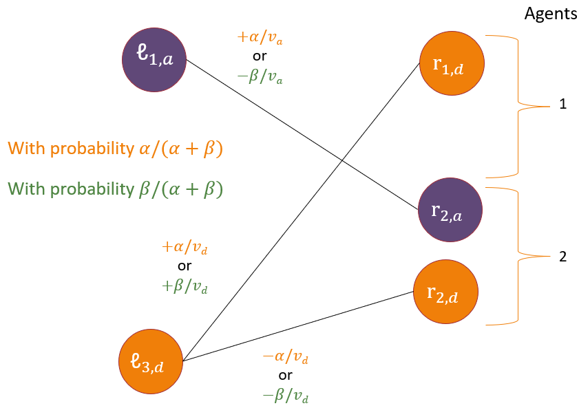
Now we shed light on what we mean by carefully rounding the paths of the CCC/CCW $\mathcal{P}$ . But first we build some intuition. Focus on $t_{p}$ and $s_{p+1}$ for some fixed $1\leq p\leq q$ in case of a CCC (or $p<q$ in the case of a CCW). Since $t_{p}\sim s_{p+1}$ , whatever rounding procedure we use, we want the relative signs of the changes to $x^{r}(t_{p})$ and $x^{r}(s_{p+1})$ to depend on whether $t_{p}$ and $s_{p+1}$ fall on the same or different sides of $G$ (these sides being “left” and “right” corresponding to vertex sets $L$ and $R$ ; equivalently, left and right of “ $=$ ” in (1d)). This way (1d) is preserved after rounding. Likewise, the magnitudes of fractional degree changes to $t_{p}$ and $s_{p+1}$ must be balanced depending on $v_{p}$ and $v_{p+1}$ so that (1d) is preserved for $i$ corresponding to $t_{p},s_{p+1}\in\kappa(i)$ . Intuitively, we round $\mathcal{P}$ carefully (1d) by ensuring i) the signs of the changes depend on which side of the equation tehy appear on, and ii), the magnitudes of said changes are weighted by the values of the items they represent. We make this precise via roundable colorings. If $a$ and $b$ are vertices belonging to different sides of the graph, we say $a\perp b$ ; otherwise we say $a\not\perp b$ .

Definition 0 (Roundable coloring).

The CCC $\mathcal{P}=$ $\langle s_{i}\leadsto t_{i}\rangle_{i\in[q]}$ has a roundable coloring if there exists $f:V(\mathcal{P})\to\{-1,1\}$ such that i) for all $i\in[q]$ , $f(s_{i})=f(t_{i})$ if and only if $s_{i}\perp t_{i}$ ; and ii) for all $i\in[q]$ , $f(t_{i})=f(s_{i+1})$ if and only if $t_{i}\perp s_{i+1}$ . A roundable coloring for a CCW is defined the same way except ii) becomes $\forall i\in[q-1]$ , $f(t_{i})=f(s_{i+1})$ if and only if $t_{i}\perp s_{i+1}$ .

Property i) will ensure $a,b\in V(\mathcal{P})$ see same-sign fractional degree change if and only if $f(a)=f(b)$ , which happens if and only if they appear on the same side (1d). Property ii) is equivalent to Remark 1 and verifies each $s_{i}\leadsto t_{i}$ is roundable in GKPS-DR-inspired manner.

Lemma 5.0.

Every CCC and CCW admits an efficiently computable roundable coloring $f$ .

Proof of Lemma 7.

Consider the following heuristic to find a roundable coloring of $\mathcal{P}=\langle s_{i}\leadsto t_{i}\rangle_{i\in[q]}$ . Assign an arbitrary color to $s_{1}$ , say $f(s_{1})=1$ . Because $f$ only has two colors, this immediately determines the color of $t_{1}$ , which depends on whether $s_{1}$ and $t_{1}$ are same-side vertices. Again, this immediately determines the color of $s_{2}$ , which in turn determines the color of $t_{2}$ , and so on.

If $\mathcal{P}$ is a CCW then $s_{1}$ and $t_{q}$ are partnerless so their colors do not affect the first property. The vertices are colored in the order $s_{1},t_{1},s_{2},t_{2},\dots,s_{q},t_{q}$ ensuring that both properties hold. Therefore, this scheme produces a roundable coloring for CCW’s in time $\mathcal{O}(|L|+|R|)$ .

Instead suppose $\mathcal{P}$ is a CCC. It only remains to check that $f(t_{q})=f(s_{1})$ . We now verify this. Observe that the greedy algorithm ensures

\forall i\in[q],\;f(t_{i})=f(s_{i})\cdot(-1)^{\mathbbm{1}(t_{i}\perp s_{i})}

and

\forall i\in[q-1],\;f(s_{i+1})=f(t_{i})\cdot(-1)^{\mathbbm{1}(t_{i}\not\perp s_{i+1})}

where $\mathbbm{1}(\cdot)$ equals 1 if “ $\cdot$ ” is true and 0 otherwise; this is a slight abuse of notation since $\perp$ is a relation but we are treating it as a boolean function. Expanding by repeated application of the above observations, we have

	$\displaystyle f(t_{q})$	$\displaystyle=f(s_{1})\cdot(-1)^{\sum_{i\in[q]}\mathbbm{1}(t_{1}\not\perp s_{i})+\sum_{i\in[q-1]}\mathbbm{1}(t_{i}\not\perp s_{i+1})}$
		$\displaystyle=f(s_{1})\cdot(-1)^{p+\psi_{q-1}}$

where $p$ is the number of same-side paths and $\psi_{q-1}$ is the number of same-side partners not counting the pair $t_{q}$ and $s_{1}$ . Then ensuring we have a roundable coloring reduces to ensuring that $t_{q}\perp s_{1}\implies p+\psi_{q-1}$ is even and $t_{q}\not\perp s_{1}\implies p+\psi_{q-1}$ is odd. Letting $\psi$ be the total number of same-side partners, the above is equivalent to asking $p+\psi$ be even, which we now prove.

Let $d$ be the number of different-side paths, and let $c_{L}$ , $c_{R}$ , $c_{LR}$ respectively be the number of left-left, right-right, and left-right partner pairs. So,

(3)

p+d=q=\psi+c_{LR}.

Let $n_{L}$ be the number of left vertices in the CCC. Clearly, $n_{L}=2c_{L}+c_{LR}$ . Look at $n_{L}-d$ , this is the number of left vertices remaining after removing the different-side paths in $\langle s_{i}\leadsto t_{i}\rangle_{i\in[q]}$ . Since these vertices must be covered by same side paths we must have $n_{L}-d$ even. Then, with all congruences taken modulo $2$ ,

0\equiv n_{L}-d=2c_{L}+c_{LR}-d\equiv c_{LR}-d.

Plugging the above into (3) gives $p=\psi+c_{LR}-d\equiv\psi$ . Therefore, $\psi+p\equiv\psi+\psi\equiv 0$ . ∎

5.3.2. Using roundable colorings

Roundable colorings will ensure the sings of changes are as desired. We now introduce notation to use the roundable colorings and ensure that the magnitudes of said changes is done in proportion to the value of items involved.

Although the notation used next is cumbersome, the intuition is to fix $\alpha,\beta>0$ “small enough” that all edge variables stay in $[0,1]$ and vertex fractional degrees stay within their current ceilings and floors but “large enough” that at least one edge or vertex is settled. First, fix the roundable coloring $f$ , which is possible per Lemma 7. Next, decompose each path $s_{i}\leadsto t_{i}$ into alternating matchings $M_{-1}^{i}$ and $M_{1}^{i}$ such that $\forall a\in\{s_{i},t_{i}\},\;\exists e\in M_{f(a)}^{i}$ such that $e\in N(a)$ ; property ii) of $f$ guarantees this is possible. In other words, vertex $a\in\{s_{i},t_{i}\}$ is present in $M_{f(a)}^{i}$ . For readability drop the $r$ superscripts briefly and let

	$\displaystyle\Gamma_{-1}^{i}(\gamma)\equiv$	$\displaystyle\bigvee_{e\in M_{-1}^{i}}(x_{e}+\gamma=1)\vee\bigvee_{e\in M_{1}^{i}}(x_{e}-\gamma=0)$
		$\displaystyle\vee\bigvee_{a\in\{s_{i},t_{i}\}}(f(a)=-1\implies x(a)+\gamma=\lceil x(a)\rceil)\phantom{\Gamma_{-1}^{i}(\gamma)\equiv}$
(4)			$\displaystyle\vee\bigvee_{a\in\{s_{i},t_{i}\}}(f(a)=1\implies x(a)-\gamma=\lfloor x(a)\rfloor),$

and, symmetrically,

	$\displaystyle\Gamma_{1}^{i}(\gamma)\equiv$	$\displaystyle\bigvee_{e\in M_{1}^{i}}(x_{e}+\gamma=1)\vee\bigvee_{e\in M_{-1}^{i}}(x_{e}-\gamma=0)$
		$\displaystyle\vee\bigvee_{a\in\{s_{i},t_{i}\}}(f(a)=1\implies x(a)+\gamma=\lceil x(a)\rceil)$
(5)			$\displaystyle\vee\bigvee_{a\in\{s_{i},t_{i}\}}(f(a)=-1\implies x(a)-\gamma=\lfloor x(a)\rfloor).$

Finally, the magnitudes fixed (in analogy to Section 2) are

(6)

\alpha:=\min\left\{\gamma>0:\bigvee_{i\in[q]}\Gamma_{-1}^{i}\left(\frac{1}{v_{i}}\gamma\right)\right\},\;\beta:=\min\left\{\gamma>0:\bigvee_{i\in[q]}\Gamma_{1}^{i}\left(\frac{1}{v_{i}}\gamma\right)\right\}.

Both $\alpha$ and $\beta$ are well defined as they are the minima of non-empty finite sets. The update proceeds probabilistically as follows: $\forall i\in[q],\forall e\in s_{i}\leadsto t_{i}$ ,

(7)

\text{w.p.}\;\frac{\beta}{\alpha+\beta},\;x_{e}^{r+1}=\begin{cases}x_{e}^{r}+\frac{1}{v_{i}}\alpha,&e\in M_{-1}^{i}\\ x_{e}^{r}-\frac{1}{v_{i}}\alpha,&e\in M_{1}^{i}\end{cases};

(8)

\text{else, w.p.}\;\frac{\alpha}{\alpha+\beta},\;\;x_{e}^{r+1}=\begin{cases}x_{e}^{r}-\frac{1}{v_{i}}\beta,&e\in M_{-1}^{i}\\ x_{e}^{r}+\frac{1}{v_{i}}\beta,&e\in M_{1}^{i}\end{cases}.

At a high level $\alpha$ and $\beta$ are large enough that every rounding iteration at least one vertex or edge is settled. Adding the $\pm\frac{1}{v_{i}}$ terms ensures term appearing in (1d) will cancel out nicely, as seen in the proof of Lemma 9.

5.4. Algorithm analysis

Proof sketch of Theorem 3

Except for (J2), the proofs for the invariants are almost identical to those in (Gandhi et al., 2006). This is because BarterDR is crafted so as to be similar to GKPS-DR in the ways necessary for this analysis to carry over. Owing to proofs’ similarities, we defer their full treatment to Appendix B. The proof proceeds via the following invariants maintained at each iteration $r$ of BarterDR.

(J1)

$\forall e\in E$ , $\mathbb{E}[x_{e}^{r}]=x_{e}^{0}$ .
(J2)

$\forall a\in L\cup R$ and with probability 1, $\lfloor x^{0}(a)\rfloor\leq x^{r}(a)\leq\lceil x^{0}(a)\rceil$ .
(J3)

$\forall a\in L\cup R,\;\forall S\subseteq N(a),\;\forall c\in\{0,1\}$ , $\mathbb{E}[\prod_{e\in S}x_{e}^{r+1}]\leq\mathbb{E}[\prod_{e\in S}x_{e}^{r}]$ .

The main place where our proof deviates results from BarterDR choosing $\alpha$ and $\beta$ differently. In particular, GKPS-DR selects a single path and at least one of its edges becomes settled each iteration. In BarterDR the guarantee says, among all paths of the fixed CCC/CCW, at least one edge or vertex becomes settled each iteration.

Lemma 5.0.

BarterDR achieves optimal objective in expectation and $\forall i\in[n],\;\mathbb{E}[D_{i}]=0$ .

Proof of Lemma 8.

Given a $\mathsf{BarterSV}$ instance, let $\operatorname{OPT_{IP}}$ and $\operatorname{OPT_{LP}}$ be the optimal objectives of the corresponding IP (1) and the corresponding $\mathsf{BarterSV\text{-}LP}$ . Let $\{X_{e}^{*}\}_{e\in E}$ and $\{x_{e}^{*}\}_{e\in E}$ be optimal solutions to the IP and LP, respectively. Then $\operatorname{OPT_{IP}}=\sum_{e\in E}w_{e}X_{e}^{*}\leq\sum_{e\in E}w_{e}x_{e}^{*}=\operatorname{OPT_{LP}}$ . Per Theorem 3, BarterDR satisfies (P1) when rounding $\{x_{e}^{*}\}_{e\in E}$ to $\{X_{e}\}\in\{0,1\}^{|E|}$ . Therefore, $\mathbb{E}[\sum_{e\in E}w_{e}X_{e}]=\sum_{e\in E}w_{e}\mathbb{E}[X_{e}]=\sum_{e\in E}w_{e}x_{e}^{*}=\operatorname{OPT_{LP}}$ .

By the linearity of expectation and (P1),

	$\displaystyle\mathbb{E}[D_{i}]$	$\displaystyle=\mathbb{E}[\sum_{a\in L_{i}}X(a)v_{a}-\sum_{b\in R_{i}}X(b)v_{b}]$
		$\displaystyle=\sum_{b\in L_{i}}\mathbb{E}[X(b)]v_{b}-\sum_{a\in R_{i}}\mathbb{E}[X(a)]v_{a}$
		$\displaystyle=\sum_{b\in L_{i}}x^{}(b)v_{b}-\sum_{a\in R_{i}}x^{}(a)v_{a}=D_{i}^{0}=0.$

The last equation follows because $\{x^{*}_{e}\}_{e\in E}$ satisfies (1d) as argued in the proof of Theorem 3. ∎

Lemma 5.0.

If $D_{i}^{r}=0$ and there exists distinct floating $a,b\in f(i)$ , then $D_{i}^{r+1}=0$ .

Proof of Lemma 9.

If no vertex from $L_{i}\cup R_{i}$ appears in the CCC/CCW’s endpoints $V(\mathcal{P}):=\bigcup_{i\in[q]}\{s_{i},t_{i}\}$ then we are done. So suppose $a\in L_{i}\cup R_{i}$ and $a\in V(\mathcal{P})$ in this $r$ -th rounding iteration. By assumption there exists another floating vertex, namely $b\in L_{i}\cup R_{i}$ in iteration $r$ when $\langle s_{i}\leadsto t_{i}\rangle_{i\in[q]}$ was constructed. Therefore, $a$ is not partnerless hence it cannot be the endpoint of a CCW so there exists $b\in V(\mathcal{P})$ such that $a\sim b$ . Moreover, by property 2 of the definition of a CCC/CCW, said $b$ is unique. Therefore, $a$ and $b$ are the only vertices in $V(\mathcal{P})$ affecting $D_{i}$ this iteration $r$ ; i.e., $\forall d\in(L_{i}\cup R_{i})-\{a,b\},\;x^{r}(d)=x^{r+1}(d)$ . Since $a\sim b$ , we may assume without loss of generality that $a=t_{k}$ and $b=s_{k+1}$ for some $k\in[q]$ (or $k\in[q-1]$ for a CCW); recall $s_{q+1}\equiv s_{1}$ . We know $f(a)=f(b)$ if and only if $a$ and $b$ belong to opposite graph sides where $f$ is the valid coloring function corresponding to $\mathcal{P}$ , which can be fixed efficiently per Lemma 7.

Consider the two possible rounding events, described in (7). Call these events $\theta_{1}$ and $\theta_{2}$ . Suppose $a$ and $b$ are opposite-side vertices, hence $f(a)=f(b)$ . Focus on event $\theta_{1}$ (the proof for $\theta_{2}$ is exactly the same but replacing $\alpha$ with $-\beta$ ). Under event $\theta_{1}$ we have

x^{r+1}(a)=x^{r}(a)-f(a)\frac{1}{v_{a}}\alpha\quad\text{and}\quad x^{r+1}(b)=x^{r}(b)-f(b)\frac{1}{v_{b}}\alpha.

A moment’s notice here shows that $x^{r+1}(a),x^{r+1}(b)\in[0,1]$ per the definitions of Sections 5.3.2, 5.3.2 and 6. Note the factor of “ $-f(a)$ ” appears because $a$ belongs to $M^{i}_{f(a)}$ for some $i$ . Conveniently, this leaves us with

(9)		$\displaystyle x^{r+1}(a)v_{a}-f(a)f(b)x^{r+1}(b)v_{b}$	$\displaystyle=x^{r}(a)v_{a}-f(a)f(b)x^{r}(b)v_{b}-f(a)\alpha+f(a)\alpha$
(10)			$\displaystyle=x^{r}(a)v_{a}-f(a)f(b)x^{r}(b)v_{b},$

using the fact $f(b)\cdot f(b)=1$ . Without loss of generality let $a\in L_{i}$ . Therefore, expanding $D_{i}^{r+1}$ :

(11)

D_{i}^{r+1}=\sum_{s\in L_{i}}x^{r+1}(s)v_{t}-\sum_{t\in R_{i}}x^{r+1}(t)v_{t}.

Having fixed $a\in L_{i}$ , we know $f(a)f(b)=1$ if and only if $b\in R_{i}$ . Thus, take out $x^{r+1}(a)$ and $x^{r+1}(b)$ from the sums and substitute (10) to have

(12)

\sum_{s\in L_{i}-\{a,b\}}x^{r+1}(s)v_{t}-\sum_{t\in R_{i}-\{b\}}x^{r+1}(t)v_{t}+x^{r}(a)v_{a}-f(a)f(b)x^{r}(b)v_{b}.

Now observe that $x^{r+1}(p)=x^{r}(p)$ for all $p\in(L_{i}\cup R_{i})-\{a,b\}$ . Moreover, $b\in R_{i}$ if and only if $f(a)f(b)=1$ , so we can reabsorb the terms “ $x^{r}(a)v_{a}$ ” and “ $x^{r}(b)v_{b}$ ” into their respective summations; thus yielding $\sum_{s\in L_{i}}x^{r}(s)v_{t}-\sum_{t\in R_{i}}x^{r}(t)v_{t}$ . But this is precisely $D_{i}^{r}$ , which we’ve assumed to be 0. ∎

Proof of Theorem 1.

It is straightforward to check that after solving $\mathsf{BarterSV\text{-}LP\text{-}Caps}$ there are at most $|E|$ floating edges. Each iteration of the pre-processing step finds a cycle, say using depth-first-search, and rounds said cycle in time $\mathcal{O}(|L|+|R|)$ with at least one edge being settled every time a cycle is rounded. Therefore, the pre-processing step takes time at most $\mathcal{O}(|E|\cdot(|L|+|R|))$ . Similarly, FindCCC takes time $\mathcal{O}(|L|+|R|)$ to find and round a CCC or CCW. Each iteration a CCC/CCW is rounded either one edge or vertex becomes settled. Therefore BarterDR runs in time $\mathcal{O}((|L|+|R|)\cdot(|L|+|R|+|E|))$ .

Let $D_{i}^{r}$ be $D_{i}$ like in (2) but with variables $x_{e}^{r}$ instead of $X_{e}$ . Then Lemma 9 guarantees that for each agent $i$ , $D_{i}^{r}=0$ implies $D_{i}^{r+1}=0$ until $L_{i}\cup R_{i}$ has exactly one floating vertex (if this happens at all). This means if in some iteration the number of floating vertices in $L_{i}\cup R_{i}$ went from at least 2 to 0, then $D_{i}=0$ by the degree preservation invariant (J2), proved in the proof of Theorem 3, and we are done. Therefore, the only case we must consider is when there is a solitary floating vertex $d\in L_{i}\cup R_{i}$ . Let $t^{\prime}$ be the first iteration that started with $L_{i}\cup R_{i}$ having a sole vertex $d$ with $x^{t^{\prime}}(d)\not\in\mathbb{Z}$ . Then by expanding

(13)	$\displaystyle D_{i}$	$\displaystyle\leq\left\|\sum_{a\in L_{i}}v_{a}X(a)-\sum_{b\in R_{i}}v_{b}X(b)\right\|$
(14)		$\displaystyle=\left\|\sum_{a\in L_{i}}v_{a}X(a)-\sum_{a\in L_{i}}v_{a}x^{t^{\prime}}(a)+\sum_{b\in R_{i}}v_{b}x^{t^{\prime}}(b)-\sum_{b\in R_{i}}v_{b}X(b)\right\|$
(15)		$\displaystyle=\left\|\sum_{a\in L_{i}}v_{a}(X(a)-x^{t^{\prime}}(a))+\sum_{b\in R_{i}}v_{b}(x^{t^{\prime}}(b)-X(b))\right\|$
(16)		$\displaystyle\leq\sum_{a\in(L_{i}\cup R_{i})-\{d\}}v_{a}\left\|X(a)-x^{t^{\prime}}(a)\right\|+v_{d}\left\|x^{t^{\prime}}(d)-X(d)\right\|$
(17)		$\displaystyle<v_{d}\leq v_{i}^{*},$

which is our desired $D_{i}$ bound for Theorem 1. Equation (14) follows because we assume $D_{i}^{1}=0$ (as $D_{i}^{0}$ corresponds to the LP solution and the pre-processing step thus guarantees $D_{i}^{1}=0$ ) and $t^{\prime}$ is the first iteration where $L_{i}\cup R_{i}$ contains exactly one floating vertex; therefore, by induction and Lemma 9, $D_{i}^{t^{\prime}}=0$ . Inequality (16) follows from the triangle inequality. The strict inequality in (17) follows because $d$ was the sole floating vertex of $L_{i}\cup R_{i}$ in iteration $t^{\prime}$ ; hence by Lemma 2, $\forall a\in(L_{i}\cup R_{i})-\{d\},\;X(a)-x^{t^{\prime}}(a)=0$ and $|x^{t^{\prime}}(d)-X(d)|<1$ .

By assumption, $D_{i}^{1}=0$ for all $i$ since $\{x_{e}^{0}\}_{e\in E}$ is an optimal solution to the corresponding $\mathsf{BarterSV\text{-}LP}$ and the pre-processing step ensures $D_{i}^{0}=0\implies D_{i}^{1}=0$ . Then, by Lemma 9, the only $D_{i}$ ’s that are not necessarily preserved are those where $L_{i}\cup R_{i}$ ends up with exactly one floating vertex in some algorithm iteration $t^{\prime}$ . As argued above, this case leads to $D_{i}<v_{i}^{*}$ . Together with Lemma 8 this completes the proof. ∎

Consequently from Theorems 1 and 3:

Corollary 0.

$\mathsf{BarterSV\text{-}LP}$ with all items having equal values is integral.

To see this note that if all item values are equal then setting them all equal to $1$ gives an equivalent $\mathsf{BarterSV}$ instance with $v^{*}=1$ . Then the $D_{i}<v^{*}$ guarantee recovers $D_{i}=0$ . In this special case, our randomized algorithm recovers an integral solution to the LP, proving its integrality.

6. Extension of $\mathsf{BarterSV}$ to multiple copies of each item

In Section 1.1 we formulated $\mathsf{BarterSV}$ where each agent has and wants at most one copy of any item $j\in\mathcal{I}$ . We now consider $\mathsf{BarterSV\text{-}Caps}$ the natural generalization where agents may swap an arbitrary number item copies. In addition to the previous inputs, for each agent $i\in\mathcal{N}$ , we take capacity functions $\eta_{i}:\mathcal{I}\to\mathbb{Z}^{+}$ and $\omega_{i}:\mathcal{I}\to\mathbb{Z}^{+}$ denoting the (non-negative) number of copies owned and desired of each $j\in\mathcal{I}$ . For simplicity we define $\eta(j)=0$ for $j\not\in H_{i}$ and $\omega_{i}(j)=0$ for $j\not\in W_{i}$ . Analogously, now $g:\mathcal{N}\times\mathcal{N}\times\mathcal{I}\to\mathbb{Z}^{+}$ and $g(i,i^{\prime},j)=k$ says agent $i$ gives $k$ copies of item $j$ to agent $i^{\prime}$ . Much like before, a valid allocation is one where each agent $i\in\mathcal{N}$ (i) receives only desired items within capacity, meaning $\sum_{i^{\prime}\in\mathcal{N}}g(i^{\prime},i,j)\leq\omega_{i}(j)$ ; and (ii) gives away only items they possess within capacity, thus $\sum_{i^{\prime}\in\mathcal{N}}g(i,i^{\prime},j)\leq\eta_{i}(j)$ . The goal of $\mathsf{BarterSV\text{-}Caps}$ remains the same: to find a valid allocation of maximum utility (now defined as $\sum_{i\in\mathcal{N}}\sum{i^{\prime}\in\mathcal{N}}\sum_{j\in\mathcal{I}}w(i,i^{\prime},j)g(i,i^{\prime},j)$ ) subject to no agent giving away more value than they receive (where the values given and received by agent $i$ are now $\sum{i^{\prime}\in\mathcal{N}}\sum_{j\in\mathcal{I}}v_{j}g(i,i^{\prime},j)$ and $\sum{i^{\prime}\in\mathcal{N}}\sum_{j\in\mathcal{I}}v_{j}g(i^{\prime},i,j)$ , respectively).

Like before, $\mathsf{BarterSV\text{-}Caps}$ admits the following similar IP formulation with LP relaxation $\mathsf{BarterSV\text{-}LP\text{-}Caps}$ after relaxing (18e). For $e=(\ell_{i,j},r_{i^{\prime},j})$ we relax $y_{e}$ to be in $[0,\min\{\eta_{i}(j),\omega_{i^{\prime}}(j)\}]$ .


(18a)	$\displaystyle\max\quad$	$\displaystyle\sum_{e\in E}w_{e}x_{e}$
(18b)	subj. to	$\displaystyle x(\ell_{ij})\leq\eta_{i}(j),$	$\displaystyle i\in[n],\ell_{ij}\in L_{i}$
(18c)		$\displaystyle x(r_{ij})\leq\omega_{i}(j),$	$\displaystyle i\in[n],r_{ij}\in R_{i}$
(18d)		$\displaystyle\sum_{a\in L_{i}}x(a)v_{a}=\sum_{b\in R_{i}}x(b)v_{b},$	$\displaystyle i\in[n]$
(18e)		$\displaystyle x_{e}\in\mathbb{Z}^{+},$	$\displaystyle e=(\ell_{ij},r_{i^{\prime}j})\in E$	.

6.1. Equivalence of $\mathsf{BarterSV}$ -Caps with single item copies

By explicitly making distinct items for each capacitated item in a $\mathsf{BarterSV\text{-}Caps}$ instance we can reduce said instance to one of $\mathsf{BarterSV}$ . Although, the resulting $\mathsf{BarterSV}$ and $\mathsf{ValBalMatching}$ formulation now has a number of vertices exponential in the size of the input, this is not a problem. We only use this $\mathsf{BarterSV}$ instance as a thought experiment to establish that BarterDR will give correct output. To avoid solving any large instances we first solve the polynomial-sized $\mathsf{BarterSV\text{-}LP\text{-}Caps}$ and subsequently observe BarterDR actually has polynomial size input in Lemma 2.

Lemma 6.0.

Any instance of $\mathsf{BarterSV\text{-}Caps}$ has a corresponding (larger but) equivalent $\mathsf{BarterSV}$ instance with unit capacities.

Proof of Lemma 1.

The instance with unit copies of each item will be large but it is only a thought experiment; we do not directly solve the corresponding LP nor write the full graph down. Fix an agent $i$ and an item $j$ in $H_{i}$ . Make $\eta_{i}(j)$ copies of this vertex each with unit capacity, say $\ell_{ij1},\ell_{ij2},\dots,\ell_{ij\eta_{i}(j)}$ . Similarly, for an item $j^{\prime}\in W_{i}$ , make $\omega_{i}(j^{\prime})$ copies $r_{ij^{\prime}1},r_{ij^{\prime}2},\dots,r_{ij^{\prime}\omega_{i}(j^{\prime})}$ . Like before add edges between all vertices corresponding to the same original items. Keep all edge weights the same and use the same corresponding weights for edges between copies i.e., if $e=(\ell_{ijk_{1}},r_{i^{\prime}jk_{2}})$ and $f=(\ell_{ij},\ell_{i^{\prime}j})$ then $w_{e}=w_{f}$ . Call this new set of edges over vertex copies $E^{\prime}$ .

To see the two formulations are equivalent, we show $x$ , $\forall e\in E,x_{e}\geq 0$ is feasible to $\mathsf{BarterSV\text{-}LP\text{-}Caps}$ if and only if $z$ , $\forall e\in E^{\prime},z_{e}\in[0,1]$ is feasible to $\mathsf{BarterSV\text{-}LP}$ . Moreover, $x$ and $z$ have the same objective value. Let $e=(\ell_{ij},r_{i^{\prime}j})$ then $x_{e}=k+r$ for $k\in\mathbb{Z}^{+}$ and $0\leq r<1$ . Correspondingly let $e_{p}=(\ell_{ijp},r_{i^{\prime}jp})\in E^{\prime}$ and set $z_{e_{1}},z_{e_{2}},\dots,z_{e_{k}}$ all equal to $1$ and $z_{e_{k+1}}=r$ . $k+r\leq\min\{\eta_{i}(j),\omega_{i}(j)\}$ if and only if $x$ and $z$ are feasible. Moreover, both $x_{e}$ and $(z_{e_{1}},\dots,z_{e_{k+1}})$ each contribute $(k+r)w_{e}$ to the objective and $(k+r)v_{j}$ value given by agent $i$ and received by agent $i^{\prime}$ .

Therefore we always write and solve $\mathsf{BarterSV\text{-}LP\text{-}Caps}$ and use $\mathsf{BarterSV\text{-}LP}$ only as a thought experiment to facilitate the presentation of the problem. It is straightforward to check that the size of $\mathsf{BarterSV\text{-}LP\text{-}Caps}$ is $\operatorname{poly}(|\mathcal{I}|,n,\log\eta,\log\omega)$ where $\eta=\max_{i\in[n],j\in H_{i}}\eta_{i}(j)$ and similarly $\omega=\max_{i\in[n],j\in H_{i}}\omega_{i}(j)$ . ∎

Let $E^{\prime}$ correspond to the graph with vertex copies as outlined in the proof of Lemma 1.

Lemma 6.0.

A solution $\{y_{e}\}_{e\in E^{\prime}}$ to $\mathsf{BarterSV\text{-}LP}$ has at most $|E|$ floating variables.

Proof of Lemma 2.

Like in the proof of Lemma 1, corresponding to each group of $z_{e_{1}},z_{e_{2}},\dots$ there is at most one $z_{e_{p}}=r$ for $0<r<1$ . Therefore, the number of floating edges is at most $|E|$ . ∎

In conclusion, by Lemmas 1 and 2, BarterDR is also an efficient algorithm for the more general $\mathsf{BarterSV\text{-}Caps}$ .

7. Fairness

Fairness is an important consideration when resource allocation algorithms are deployed in the real-world. Theorem 3 allows for adding fairness constraints to $\mathsf{BarterSV\text{-}LP}$ . Previous works such as (Duppala et al., 2023; Esmaeili et al., 2022, 2023) studied various group fairness notions, and formulated the fair variants of problems like Clustering, Set Packing, etc., by adding fairness constraints to the Linear Programs of the respective optimization problems.

Consider a toy example of such an approach where we are given $\ell$ communities $G_{1},\dots,G_{\ell}\subseteq[n]$ of agents coming together to thicken the market. In order to incentivize said communities to join the centralized exchange, the algorithm designer may promise that each community $G_{p}$ will receive at least $\mu_{p}$ units of value on average. By adding the constraints

(19)

\sum_{i\in G_{p}}x(r_{ij})v_{j}\geq\mu_{p},\quad p\in[\ell]

to the $\mathsf{BarterSV\text{-}LP}$ , the algorithm designer ensures that the expected utility of each group $G_{p}$ is at least $\mu_{p}$ . More precisely, (P1) and the linearity of expectation ensures

	$\displaystyle\mathbb{E}[\sum_{i\in G_{p}}X(r_{ij})v_{j}]$	$\displaystyle=\sum_{i\in G_{p}}\mathbb{E}[X(r_{ij})]v_{j}$
		$\displaystyle=\sum_{i\in G_{p}}x(r_{ij})v_{j}\geq\mu_{p}.$

The same rationale can be extended to provide individual guarantees (in expectation) by adding analogous constraints for each agent. We conclude this brief discussion by highlighting the versatility of LPs and, as a result, of BarterDR.

8. Hardness of $\mathsf{BarterSV}$

We first prove Theorem 2: it is NP-Hard to find any non-empty allocation satisfying $D_{k}=0$ for all agents $k$ . By non-empty we mean the corresponding LP solution $x\neq 0$ , i.e., at least one agent gives away an item. The proof proceeds by reducing from the NP-hard problem of Partition.

Definition 0 (Partition).

A Partition instance takes a set $S=\{a_{1},a_{2},\dots,a_{n}\}$ of $n$ positive integers summing to an integer $2T$ . The goal of Partition is to determine if $S$ can be partitioned into disjoint subsets $S_{1}$ and $S_{2}$ such that each subset sums exactly to an integer $T$ .

Lemma 8.0.

Given a Partition instance, it can be reduced in polynomial time to a corresponding $\mathsf{BarterSV}$ instance with two agents.

Proof.

Consider an instance $I=(S,2T)$ of partition problem where $S=\{a_{1},a_{2},\dots,a_{n}\}$ is a set of integers where $\sum_{i\in[n]}a_{i}=2T$ . Given $I$ , the corresponding $\mathsf{BarterSV}$ instance is constructed as follows.

Let the set of items $\mathcal{I}=\{i_{1},i_{2},\dots,i_{n},i_{n+1}\}$ with item values $v_{j}:=a_{j}$ for each item $i_{j},j\in[n]$ and $v_{n+1}:=T$ for item $i_{n+1}$ . There are only two agents. Agent $1$ has item lists $H_{1}:=\{i_{1},\dots,i_{n}\}$ and $W_{1}:=\{i_{n+1}\}$ . Symmetrically, agent $2$ has item lists $W_{2}:=\{i_{j}:j\in[n]\}$ and $H_{2}:=\{i_{n+1}\}$ . The particular weights $w_{e}$ of allocating items (i.e., allocation’s utility) do not matter as we only care about whether some non-empty allocation exists. ∎

Recall the goal is to show there exists a non-empty allocation such that for each agent $k\in[2]$ , $D_{k}=0$ if and only if the corresponding Partition instance has a solution.

Lemma 8.0.

There exists a polynomial time algorithm to find a non-empty allocation of items with $D_{k}=0$ for each agent $k$ in the $\mathsf{BarterSV}$ instance if and only if there exists a polynomial time algorithm to the corresponding Partition instance.

Proof.

Forward direction (Partition $\implies$ $\mathsf{BarterSV}$ ). Given a solution $(S_{1},S_{2})$ to the Partition instance, the corresponding $\mathsf{BarterSV}$ instance has a solution in the following manner. Allocate the items $\{i_{j}:j\in S_{1}\}\subseteq H_{1}$ to agent $2$ and allocate the item $i_{n+1}\in H_{2}$ to agent $1$ . Thus, the value of the items received and given by both the agents is exactly $T$ resulting in a non-empty allocation with $D_{1}=D_{2}=0$ .

Backward Direction ( $\mathsf{BarterSV}$ $\implies$ Partition). Take a non-empty allocation of items $\mathcal{I}$ to each agent $k\in[2]$ with $D_{k}=0$ . Such a non-empty allocation must have agent $1$ giving away their only item, which has value $T$ . Therefore $D_{1}=0$ implies agent $1$ received $T$ units of value. Let the items agent $1$ received be $i_{j_{1}},i_{j_{2}},\dots,i_{j_{\ell}}$ , letting $J=\{j_{1},\dots,j_{\ell}\}$ . Thus, $\sum_{p\in J}v_{p}=T$ . Therefore, the corresponding partition instance has solution $S_{1}=\{a_{p}:p\in J\}$ and $S_{2}=\{a_{p}:p\not\in J\}$ . ∎

Together, Lemmas 2 and 3 prove Theorem 2: it is NP-hard to find a non-empty allocation of items with $D_{k}=0$ for any agent $k$ .

8.1. LP approaches will not beat $D_{i}<v^{*}$

A natural follow-up question: is it possible to guarantee $D_{i}<v^{*}-\epsilon$ for some $\epsilon>0$ ? At least using $\mathsf{BarterSV\text{-}LP}$ , this is not be possible. Consider the family of $\mathsf{BarterSV}$ instances $\Pi(n)$ wherein two agents have one item each and desire each other’s item. The agent’s items are $j_{1}$ and $j_{2}$ , respectively, with values $v_{j_{1}}=1$ and $v_{j_{2}}=1/n$ . Let the utility be that of maximizing the total value reallocated (i.e., for $e=(a,b)$ , $w_{e}=v_{a}=v_{b}$ , $\forall e\in E$ in the corresponding VBM instance). The LP solution corresponds to agent 1 giving a $1/n$ -fraction of her item away and agent 2 giving his entire item away for an optimal objective value of $2/n$ . Even if agent $2$ always gives his item away, the objective achieved is only $1/n$ . Therefore, to achieve the optimal objective agent $1$ must give away her item with positive probability. This leads to the worst case, $D_{1}\geq 1-1/n=v^{*}-1/n$ . Therefore,

Remark 2.

For any $\epsilon>0$ , there exists $n$ such that $\Pi(n)$ achieves $D_{i}\geq v^{*}-\epsilon$ .

A moment’s reflection makes it clear that the only feasible (integral) reallocation to this family of instances is the empty reallocation i.e., the zero vector. A direction to bypass this ”integrality gap”-like barrier in $D_{i}$ might be to write $\mathsf{BarterSV\text{-}LP}$ only for instances in which we know $D_{i}=0$ has a feasible non-empty integral reallocation. However, this is in and of itself a hard problem as proved in Theorem 2.

9. Conclusion

We introduce and study $\mathsf{BarterSV}$ , a centralized barter exchange problem where each item has a value agreed upon by the participating agents. The goal is to find an allocation/exchange that (i) maximizes the collective utility of the allocation such that (ii) the total value of each agent’s items before and after the exchange is equal. Though it is NP-hard to solve $\mathsf{BarterSV}$ exactly, we can efficiently compute allocations with optimal expected utility where each agent’s net value loss is at most a single item’s value. Our problem is motivated by the proliferation of large scale web markets on social media websites with 50,000-60,000 active users eager to swap items with one another. We formulate and study this novel problem with several real-world exchanges of video games, board games, digital goods and more. These exchanges have large communities, but their decentralized nature leaves much to be desired in terms of efficiency.

Future directions of this work include accounting for arbitrary item valuations i.e., different agents may value items differently. Directly applying our algorithm does not work because we rely on the paths of $G$ consisting of items with all-equal values. Additionally, we briefly touch on how some fairness criteria interact with our model algorithm; however, the exploration of many important fairness criteria is left for future work. Finally, we argue why our specific LP-based approach cannot guarantee better than $D_{i}<v^{*}$ . It remains an open question whether other approaches (LP-based or not) can beat this bound or whether improving this result is NP-hard altogether.

Acknowledgements.

Sharmila Duppala, Juan Luque and Aravind Srinivasan are all supported in part by NSF grant CCF-1918749.

References

(1)
Abbassi et al. (2013) Zeinab Abbassi, Laks V. S. Lakshmanan, and Min Xie. 2013. Fair Recommendations for Online Barter Exchange Networks. In International Workshop on the Web and Databases.
Abraham et al. (2007) David J. Abraham, Avrim Blum, and Tuomas Sandholm. 2007. Clearing Algorithms for Barter Exchange Markets: Enabling Nationwide Kidney Exchanges. In Proceedings of the 8th ACM Conference on Electronic Commerce (EC ’07). Association for Computing Machinery, New York, NY, USA, 295–304. https://doi.org/10.1145/1250910.1250954
Ashlagi et al. (2018) Itai Ashlagi, Adam Bingaman, Maximilien Burq, Vahideh Manshadi, David Gamarnik, Cathi Murphey, Alvin E. Roth, Marc L. Melcher, and Michael A. Rees. 2018. Effect of Match-Run Frequencies on the Number of Transplants and Waiting Times in Kidney Exchange. American Journal of Transplantation 18, 5 (2018), 1177–1186. https://doi.org/10.1111/ajt.14566
Aziz et al. (2021) Haris Aziz, Ioannis Caragiannis, Ayumi Igarashi, and Toby Walsh. 2021. Fair Allocation of Indivisible Goods and Chores. Auton Agent Multi-Agent Syst 36, 1 (Nov. 2021), 3. https://doi.org/10.1007/s10458-021-09532-8
Biró et al. (2009) Péter Biró, David F. Manlove, and Romeo Rizzi. 2009. Maximum Weight Cycle Packing in Directed Graphs, with Application to Kidney Exchange Programs. Discrete Math. Algorithm. Appl. 01, 04 (Dec. 2009), 499–517. https://doi.org/10.1142/S1793830909000373
Brubach et al. (2017) Brian Brubach, Karthik Abinav Sankararaman, Aravind Srinivasan, and Pan Xu. 2017. Algorithms to Approximate Column-sparse Packing Problems. ACM Transactions on Algorithms (TALG) 16 (2017), 1 – 32.
Carvalho et al. (2021) Margarida Carvalho, Xenia Klimentova, Kristiaan Glorie, Ana Viana, and Miguel Constantino. 2021. Robust models for the kidney exchange problem. INFORMS Journal on Computing 33, 3 (2021), 861–881.
Chekuri et al. (2010) Chandra Chekuri, Jan Vondrák, and Rico Zenklusen. 2010. Dependent randomized rounding via exchange properties of combinatorial structures. In 2010 IEEE 51st Annual Symposium on Foundations of Computer Science. IEEE, 575–584.
Constantino et al. (2013) Miguel Constantino, Xenia Klimentova, Ana Viana, and Abdur Rais. 2013. New insights on integer-programming models for the kidney exchange problem. European Journal of Operational Research 231, 1 (2013), 57–68.
Duppala et al. (2023) Sharmila Duppala, Juan Luque, John Dickerson, and Aravind Srinivasan. 2023. Group Fairness in Set Packing Problems. In Proceedings of the Thirty-Second International Joint Conference on Artificial Intelligence, IJCAI-23, Edith Elkind (Ed.). International Joint Conferences on Artificial Intelligence Organization, 391–399. https://doi.org/10.24963/ijcai.2023/44 Main Track.
Esmaeili et al. (2023) Seyed Esmaeili, Sharmila Duppala, Davidson Cheng, Vedant Nanda, Aravind Srinivasan, and John P Dickerson. 2023. Rawlsian fairness in online bipartite matching: Two-sided, group, and individual. In Proceedings of the AAAI Conference on Artificial Intelligence, Vol. 37. 5624–5632.
Esmaeili et al. (2022) Seyed A. Esmaeili, Sharmila Duppala, John P. Dickerson, and Brian Brubach. 2022. Fair Labeled Clustering. https://doi.org/10.48550/arXiv.2205.14358 arXiv:2205.14358 [cs]
Fang et al. (2015) Wenyi Fang, Aris Filos-Ratsikas, Søren Kristoffer Stiil Frederiksen, Pingzhong Tang, and Song Zuo. 2015. Randomized assignments for barter exchanges: Fairness vs. efficiency. In Algorithmic Decision Theory: 4th International Conference, ADT 2015, Lexington, KY, USA, September 27–30, 2015, Proceedings. Springer, 537–552.
Farnadi et al. (2021) Golnoosh Farnadi, William St-Arnaud, Behrouz Babaki, and Margarida Carvalho. 2021. Individual Fairness in Kidney Exchange Programs. Proceedings of the AAAI Conference on Artificial Intelligence 35, 13 (May 2021), 11496–11505.
Gandhi et al. (2006) Rajiv Gandhi, Samir Khuller, Srinivasan Parthasarathy, and Aravind Srinivasan. 2006. Dependent Rounding and Its Applications to Approximation Algorithms. J. ACM 53, 3 (May 2006), 324–360. https://doi.org/10.1145/1147954.1147956
Glorie et al. (2014) Kristiaan M Glorie, J Joris van de Klundert, and Albert PM Wagelmans. 2014. Kidney exchange with long chains: An efficient pricing algorithm for clearing barter exchanges with branch-and-price. Manufacturing & Service Operations Management 16, 4 (2014), 498–512.
Herlihy (2018) Maurice Herlihy. 2018. Atomic cross-chain swaps. In ACM Symposium on Principles of Distributed Computing (PODC). 245–254.
Jevons (1879) William Stanley Jevons. 1879. The Theory of Political Economy. Macmillan and Company.
Klimentova et al. (2021) Xenia Klimentova, Ana Viana, João Pedro Pedroso, and Nicolau Santos. 2021. Fairness models for multi-agent kidney exchange programmes. Omega 102 (2021), 102333.
McElfresh et al. (2020) Duncan McElfresh, Michael Curry, Tuomas Sandholm, and John Dickerson. 2020. Improving Policy-Constrained Kidney Exchange via Pre-Screening. In Advances in Neural Information Processing Systems, Vol. 33. 2674–2685.
Noothigattu et al. (2020) Ritesh Noothigattu, Dominik Peters, and Ariel D Procaccia. 2020. Axioms for learning from pairwise comparisons. Advances in Neural Information Processing Systems 33 (2020), 17745–17754.
Plaut et al. (2016) Benjamin Plaut, John Dickerson, and Tuomas Sandholm. 2016. Fast optimal clearing of capped-chain barter exchanges. In Proceedings of the AAAI Conference on Artificial Intelligence, Vol. 30.
Thyagarajan et al. (2022) Sri AravindaKrishnan Thyagarajan, Giulio Malavolta, and Pedro Moreno-Sanchez. 2022. Universal atomic swaps: Secure exchange of coins across all blockchains. In IEEE Symposium on Security and Privacy (S&P). IEEE, 1299–1316.

Appendix A Direct application of GKPS-DR fails

Example 1 is a worst case instance where a direct application of GKPS-DR to the fractional optimal solution of $\mathsf{BarterSV}$ results in a net loss of $\sum_{j\in L_{i}}v_{j}$ for some agent $i$ ; i.e., agent $i$ gives away all their items and does not receive any item from its wishlist.

Example 0.

Consider an instance of $\mathsf{BarterSV}$ with two agents where $W_{1}=\{1,2\},W_{2}=\{3,4\}$ and $H_{1}=\{3,4\},H_{2}=\{1,2\}$ . Let the values of the items be $v(1)=v(2)=10$ and $v(3)=v(4)=20$ .

Figure 3 shows the bipartite graph of the $\mathsf{BarterSV}$ instance from Example 1. The edges are unweighted and the optimal LP solution is $x=[0.5,0.5,1,1]$ . The first two coordinates of $x$ correspond to items given by agent $1$ . GKPS-DR will round both of these co-ordinates to $0$ with positive probability thus resulting in agent $2$ incurring a net loss of $\sum_{a\in L_{2}}v_{a}=20$ units of value.

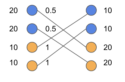
Observation 1.

GKPS-DR rounding $x$ results in the vector $X=[0,0,1,1]$ with positive probability; this is the worst case for agent $2$ where their net loss is $\sum_{a\in L_{2}}v_{a}=20$ units of value.

The above example can be easily generalized to instances with larger item-lists and more agents where some agent $i$ achieves net value loss $\sum_{a\in L_{i}}v_{a}$ with positive probability.

Appendix B Proof of Theorem 3

Lemma B.0.

BarterDR satisfies (J1).

Proof.

The property holds trivially for $r=0$ . Recall $r=1$ corresponds to the output of the pre-processing step. This fact is proved in (Gandhi et al., 2006). Therefore, focus on some fixed $r>1$ and proceed by induction. Fix $e\in E$ and the CCC/CCW to be rounded $\mathcal{P}=\langle s_{i}\leadsto t_{i}\rangle_{i\in[q]}$ . Proceed by considering the following two events.

Event $A$ : $e$ does not appear in $\mathcal{P}$ so $e$ does not change this iteration. Thus by the induction hypothesis $\mathbb{E}[x_{e}^{r+1}\mid(x_{e}^{r}=z)\wedge A]=z$ .
Event $B$ : $e$ appears in $\mathcal{P}$ , say, in path $s_{i}\leadsto t_{i}$ for a fixed $i$ . Recall values $\alpha$ and $\beta$ from (6) are fixed and $x_{e}^{r}$ is modified according to (7). Assuming $e\in M^{i}_{-1}$ then

\mathbb{E}[x_{e}^{r+1}\mid(x_{e}^{r}=z)\wedge B]=z+\frac{\alpha}{v_{i}}\left(\frac{\beta}{\alpha+\beta}\right)-\frac{\beta}{v_{i}}\left(\frac{\alpha}{\alpha+\beta}\right)=z.

The same holds if instead $e\in M^{i}_{1}$ . Hence

	$\displaystyle\mathbb{E}[x_{e}^{r+1}\mid(x_{e}^{r}=z)]$	$\displaystyle=\mathbb{E}[x_{e}^{r+1}\mid(x_{e}^{r}=z)\wedge B]\cdot\Pr(B)$
		$\displaystyle\phantom{=}+\mathbb{E}[x_{e}^{r+1}\mid(x_{e}^{r}=z)\wedge A]\cdot\Pr(A)$
		$\displaystyle=z(\Pr(A)+\Pr(B))=z.$

Let $Z$ be the set of possible values for $x_{e}^{r}$ .

	$\displaystyle\mathbb{E}[x_{e}^{r+1}]$	$\displaystyle=\sum_{z\in Z}\mathbb{E}[x_{e}^{r+1}\mid(x_{e}^{r}=z)]\cdot\Pr(x_{e}^{r}=z)$
		$\displaystyle=\sum_{z\in Z}z\cdot\Pr(x_{e}^{r}=z)=\mathbb{E}[x_{e}^{r}].$

By the IH, then $\mathbb{E}[x_{e}^{r+1}]=x_{e}^{0}$ . ∎

Lemma B.0.

BarterDR satisfies (J2).

Proof.

The property holds trivially for $r=0$ . Recall $r=1$ corresponds to the output of the pre-processing step. This fact is proved in (Gandhi et al., 2006). Therefore, focus on some fixed $r>1$ and proceed by induction. Fix $a\in L\cup R$ and the CCC/CCW to be rounded $\mathcal{P}=\langle s_{i}\leadsto t_{i}\rangle_{i\in[q]}$ . Recall $V(\mathcal{P})$ denotes the endpoints of the paths of $\mathcal{P}$ . Proceed by cases.

Case $A$ : $a\not\in V(\mathcal{P})$ . Then either $a$ does not appear in $\mathcal{P}$ or $a$ appears in $\mathcal{P}$ but with two edges incident on it. In the former case clearly $x_{a}^{r+1}=x_{a}^{r}$ . In the latter case, the change of each incident edge is equal in magnitude and opposite in sign (since one edge belongs to $M^{i}_{-1}$ and the other to $M^{i}_{1}$ ) therefore $x_{a}^{r+1}=x_{a}^{r}$ as well. Thus by the IH $\lfloor x^{0}(a)\rfloor\leq x^{r+1}(a)\leq\lceil x^{0}(a)\rceil$ .

Case $B$ : $a\in V(\mathcal{P})$ . There is a single incident edge $e\in N(a)$ . Without loss of generality, said edge belongs path $s_{i}\leadsto t_{i}$ and thus to $M^{i}_{-1}$ (the proof for $M^{i}_{1}$ is identical). Then either $x^{r+1}(a)=x^{r}(a)+\alpha/v_{i}$ or $x^{r+1}(a)=x^{r}(a)-\beta/v_{i}$ . In either case, by definition of $\alpha$ and $\beta$ (i.e., (6)), $\alpha$ and $\beta$ are small enough that $\lfloor x^{r}(a)\rfloor\leq x^{r+1}(a)\leq\lceil x^{r}(a)\rceil$ . Observe $\lfloor x^{0}(a)\rfloor=\lfloor x^{r}(a)\rfloor$ and $\lceil x^{0}(a)\rceil=\lceil x^{r}(a)\rceil$ .

Having handled exhaustive cases, the proof is complete. ∎

Lemma B.0.

BarterDR satisfies (J3).

Proof.

The property holds trivially for $r=0$ . Recall $r=1$ corresponds to the output of the pre-processing step. This fact is proved in (Gandhi et al., 2006). Therefore, focus on some fixed $r>1$ and proceed by induction. Fix a vertex $a$ and a subset of edges $S$ incident on $a$ like in (J3). Also fix the CCC/CCW to be rounded $\mathcal{P}=\langle s_{i}\leadsto t_{i}\rangle_{i\in[q]}$ . Proceed based on the following events.

Event $A$ : no edge in $S$ has its value modified. Then $\mathbb{E}[\prod_{e\in S}x^{r+1}_{e}\mid A]=\mathbb{E}[\prod_{e\in S}x^{r}_{e}\mid A]$ .

Event $B$ : two edges $e_{1},e_{2}\in S$ have their values modified. Said edges must both belong to $s_{i}\leadsto t_{i}$ , for some fixed $i$ , with one belonging to $M^{i}_{-1}$ and the other to $M^{i}_{1}$ ; say $e_{1}\in M^{i}_{1}$ and $e_{2}\in M^{i}_{-1}$ . Then

(x_{e_{1}}^{r+1},x_{e_{2}}^{r+1})=\begin{cases}(x_{e_{1}}^{r}+\alpha/v_{i},x_{e_{2}}^{r}-\alpha/v_{i})\text{ with probability }\beta/(\alpha+\beta)\\ (x_{e_{1}}^{r}-\beta/v_{i},x_{e_{2}}^{r}+\beta/v_{i})\text{ with probability }\alpha/(\alpha+\beta)\end{cases}

where $\alpha$ and $\beta$ are fixed per (6). Let $S_{1}=S-\{e_{1},e_{2}\}$ . Then

\mathbb{E}\left[\prod_{e\in S}x_{e}^{r+1}\mid(\forall e\in S,x_{e}^{r}=z_{e})\wedge B\right]=\mathbb{E}\left[x_{e_{1}}^{r}\cdot x_{e_{2}}^{r}\mid(\forall e\in S,x_{e}^{r}=z_{e})\wedge B\right]\prod_{e\in S_{1}}z_{e}.

The above expectation can be written as $(\Psi+\Phi)\prod_{e\in S_{1}}z_{e}$ , where

	$\displaystyle\Psi$	$\displaystyle=(\beta/(\alpha+\beta))\cdot(z_{e_{1}}+\alpha)\cdot(z_{e_{2}}-\alpha)\text{ and }$
	$\displaystyle\Phi$	$\displaystyle=(\alpha/(\alpha+\beta))\cdot(z_{e_{1}}-\beta)\cdot(z_{e_{2}}+\beta).$

It is easy to s how $\Psi+\Phi\leq z_{e_{1}}z_{e_{2}}$ . Thus, for any fixed $\{e_{1},e_{2}\}\subseteq S$ and for any fixed $(\alpha,\beta)$ , and for fixed values of $z_{e}$ , the following holds:

\mathbb{E}\left[\prod_{e\in S}x_{e}^{r+1}\mid(\forall e\in S,x_{e}^{r}=z_{e})\wedge B\right]\leq\prod_{e\in S}z_{e}.

Hence, $\mathbb{E}[\prod_{e\in S}x_{e}^{r+1}\mid B]\leq\mathbb{E}[\prod_{e\in S}x_{e}^{r}\mid B]$ .

Event $C$ : exactly one edge in the set $S$ has its value modified. Let $C$ denote the event that edge $e_{1}\in S$ has its value changed in the following probabilistic way

x_{e_{1}}^{r+1}=\begin{cases}x_{e_{1}}^{r}+\alpha\text{ with probability }\beta/(\alpha+\beta)\\ x_{e_{1}}^{r}-\beta\text{ with probability }\alpha/(\alpha+\beta).\end{cases}

Thus, $\mathbb{E}[x_{e_{1}}^{r+1}\mid(\forall e\in S,x_{e}^{r}=z_{e})\wedge C]=z_{e_{1}}$ . Letting $S_{1}=S-\{e_{1}\}$ , we get that $\mathbb{E}[\prod_{e\in S}x_{e}^{r+1}\mid(\forall e\in S,x_{e}^{r}=z_{f})\wedge C]$ equals

E[x_{e_{1}}^{r+1}\mid(\forall e\in S,x_{e}^{r}=z_{f})\wedge C]\prod_{e\in S_{1}}z_{e}=\prod_{e\in S}z_{e}.

Since the equation holds for any $e_{1}\in S$ , for any values of $z_{e}$ , and for any $(\alpha,\beta)$ , we have $\mathbb{E}[\prod_{e\in S}x_{e}^{r+1}\mid C]=\mathbb{E}[\prod_{e\in S}x_{e}^{r}]$ . ∎

Proof of Theorem 3.

By Lemmas 1 and 2 BarterDR satisfies (P1) and (P2). Let $T$ be the last iteration of BarterDR. From Lemma 3 we have

\Pr(\bigwedge_{e\in S}(X_{e}=1))=\mathbb{E}[\prod_{e\in S}x_{e}^{T+1}]\leq\mathbb{E}[\prod_{e\in S}x_{e}^{1}]=\prod_{e\in S}x_{e}^{0}=\prod_{e\in S}\Pr(X_{e}=1).

The proof for $c=0$ (i.e., $\Pr(X_{e}=0)$ ) is identical. Therefore, BarterDR satisfies (P3). ∎

Barter Exchange with Shared Item Valuations

Abstract.

1. Introduction

1.1. Problem formulation: 𝖡𝖺𝗋𝗍𝖾𝗋𝖲𝖵\mathsf{BarterSV}

Definition 0.

Lemma 1.0.

Proof.

Corollary 0.

1.2. LP formulation of VBM

Lemma 1.0.

Proof.

2. Preliminaries: GKPS dependent rounding

Remark 1.

3. Related work

4. Outline of our contributions and the paper

Theorem 1.

Theorem 2.

Theorem 3.

Outline of the paper

5. BarterDR: dependent rounding algorithm for 𝖡𝖺𝗋𝗍𝖾𝗋𝖲𝖵\mathsf{BarterSV}

Notation

Algorithm and analysis outline.

5.1. Pre-processing: remove cycles in GG

Lemma 5.0.

Proof.

Lemma 5.0.

Proof.

Lemma 5.0.

Proof.

5.2. Construction of CCC’s and CCW’s via FindCCC

Definition 0.

Uncrossing the half-CCWs.

Lemma 5.0.

Proof of Lemma 5.

Runtime of FindCCC

5.3. Rounding CCC’s and CCW’s

5.3.1. Roundable colorings

Definition 0 (Roundable coloring).

Lemma 5.0.

Proof of Lemma 7.

5.3.2. Using roundable colorings

5.4. Algorithm analysis

Proof sketch of Theorem 3

Lemma 5.0.

Proof of Lemma 8.

Lemma 5.0.

Proof of Lemma 9.

Proof of Theorem 1.

Corollary 0.

6. Extension of 𝖡𝖺𝗋𝗍𝖾𝗋𝖲𝖵\mathsf{BarterSV} to multiple copies of each item

6.1. Equivalence of 𝖡𝖺𝗋𝗍𝖾𝗋𝖲𝖵\mathsf{BarterSV}-Caps with single item copies

Lemma 6.0.

Proof of Lemma 1.

Lemma 6.0.

Proof of Lemma 2.

7. Fairness

8. Hardness of 𝖡𝖺𝗋𝗍𝖾𝗋𝖲𝖵\mathsf{BarterSV}

Definition 0 (Partition).

Lemma 8.0.

Proof.

Lemma 8.0.

Proof.

8.1. LP approaches will not beat Di<v∗D_{i}<v^{*}

Remark 2.

9. Conclusion

Acknowledgements.

References

Appendix A Direct application of GKPS-DR fails

Example 0.

Observation 1.

Appendix B Proof of Theorem 3

Lemma B.0.

Proof.

Lemma B.0.

Proof.

Lemma B.0.

Proof.

Proof of Theorem 3.

1.1. Problem formulation: $\mathsf{BarterSV}$

5. BarterDR: dependent rounding algorithm for $\mathsf{BarterSV}$

5.1. Pre-processing: remove cycles in $G$

6. Extension of $\mathsf{BarterSV}$ to multiple copies of each item

6.1. Equivalence of $\mathsf{BarterSV}$ -Caps with single item copies

8. Hardness of $\mathsf{BarterSV}$

8.1. LP approaches will not beat $D_{i}<v^{*}$