Baseband control of superconducting qubits with shared microwave drives
Abstract
Accurate control of qubits is the central requirement for building functional quantum processors. For the current superconducting quantum processor, high-fidelity control of qubits is mainly based on independently calibrated microwave pulses, which could differ from each other in frequencies, amplitudes, and phases. With this control strategy, the needed physical resource could be challenging, especially when scaling up to large-scale quantum processors is considered. Inspired by Kane’s proposal for spin-based quantum computing, here, we explore theoretically the possibility of baseband flux control of superconducting qubits with only shared and always-on microwave drives. In our strategy, qubits are by default far detuned from the drive during system idle periods, qubit readout and baseband flux-controlled two-qubit gates can thus be realized with minimal impacts from the always-on drive. By contrast, during working periods, qubits are tuned on resonance with the drive and single-qubit gates can be realized. Therefore, universal qubit control can be achieved with only baseband flux pulses and always-on shared microwave drives. We apply this strategy to the qubit architecture where tunable qubits are coupled via a tunable coupler, and the analysis shows that high-fidelity qubit control is possible. Besides, the baseband control strategy needs fewer physical resources, such as control electronics and cooling power in cryogenic systems, than that of microwave control. More importantly, the flexibility of baseband flux control could be employed for addressing the non-uniformity issue of superconducting qubits, potentially allowing the realization of multiplexing and cross-bar technologies and thus controlling large numbers of qubits with fewer control lines. We thus expect that baseband control with shared microwave drives can help build large-scale superconducting quantum processors.
I Introduction
For quantum processors built with superconducting qubits, both the control accuracy and the qubit number have shown steady improvement over the past two decades Kjaergaard2020 . Notably, quantum gate operations, which are generally implemented by using microwave or baseband flux pulses Krantz2019 , with errors reaching the fault-tolerant thresholds have been achieved in quantum processors with several tens of qubits Arute2019 ; Zhu2022 ; Acharya2022 ; Kim2021 . Nevertheless, it is known that fulfilling the full promises of quantum computing requires the implementation of fault-tolerant schemes, which will need the high-fidelity control of millions of qubits Fowler2012 ; Gidney2021 . In such large-scale superconducting quantum processors, the needed physical resource, such as control electronics and cooling power in cryogenic systems, could be the most challenging obstacle for achieving accurate control of qubits, let alone solving the wiring problem Frankea2019 ; Reilly2019 ; Martinis2020 and the device yield problem Hertzberg2021 ; Kreikebaum2020 .
In superconducting quantum processors each qubit has typically a different set of parameters: frequency, anharmonicity, coupling efficiency and signal attenuations in control lines. Thus, in current small-scale quantum processors, to ensure accurate qubit control, each qubit should have its dedicated control pulse with different parameter settings Kelly2018 ; Klimov2020 . This means that the microwave control pulses could differ from each other in their amplitudes, frequencies, and phases, while for the baseband flux pulse, their amplitudes could be different. Moreover, these control pulses are generated at room temperature, and then delivered to qubits in the cryogenic system through a series of attenuators and filters for suppressing harmful noises, such as thermal noise Krantz2019 ; Chen2018 ; Krinner2019 . Considering these general arguments, the physical resource for realizing qubit control could be highly related to the type of employed control. To be more specific, the microwave control and its signal synthesis are more complicated and expensive than that of the baseband flux control, for which only a single digital-to-analog converter (DAC) per qubit is needed Krantz2019 ; Chen2018 ; Krinner2019 . Moreover, given the limited available cooling power in cryogenic systems, the microwave control lines generally need the attenuation of (about at the mixing chamber plate (MXC), for which the available cooling power is smallest), leading to heating loads larger than that of the baseband flux lines (about , need no attenuation at the MXC stage) Arute2019 ; Chen2018 ; Krinner2019 . Additionally, in large-scale quantum processors, microwave control requires higher-density control lines, making it challenging to suppress the microwave crosstalk Wenner2011 ; Rosenberg2019 ; Huang2021M and thus to achieve high-fidelity qubit control. By contrast, with baseband flux control, there exists only a single control parameter, potentially allowing the application of multiplexing technologies and cross-bar technologies to address the challenges, e.g., the wiring problem, toward large-scale quantum computing Hill2015 ; Vandersypen2017 ; Veldhorst2017 ; Li2018 .
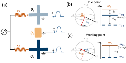
Given the above discussion, when scaling up to large-scale quantum processors, implementing baseband flux control could make requirements less stringent than that of microwave control. However, currently, microwave control is generally the essential one for implementing qubit addressing and single-qubit gate operations Motzoi2009 ; Chen2016 ; Krantz2019 , and even for two-qubit gates, such as cross-resonance gates Chow2011 . In this work, we explore theoretically the possibility of developing the baseband flux control of frequency-tunable qubits with the help of always-on shared microwave drives. It should be noted that previous works on studying baseband control of superconducting qubits mainly focus on low-frequency qubits, e.g., the composite qubit Campbell2020 and heavy-fluxonium qubit Zhang2021 , here we focus on the transmon qubits Koch2007 that have been widely used in current superconducting quantum processors. The basic idea of our control strategy is sketched in Fig. 1(a), where two qubits are coupled via a coupler and the always-on microwave drive (XY line) is shared by both qubits (in principle, can be extended to multi-qubit cases), the qubit control and the single-qubit addressing can be realized only through the flux (Z) control lines. Our work is motivated by Kane’s proposal for realizing spin-based quantum computing Kane1998 , where the spin qubit is by default off-resonance with the global always-on microwave magnetic field (i.e., at the idle point) and single-qubit gate operations are realized by tuning the spin qubit on-resonance with the field (i.e., at the working point) Wolfowicz2014 ; Laucht2015 , as shown in Figs. 1(b) and 1(c). Due to the always-on shared drive, the computational states are the basis states of the microwave-dressed qubit Liu2006 ; Zhao2022 ; Wei2022 , and accordingly, in the present work, all the qubit control are analyzed based on this microwave-dressed basis. As an example application of this baseband control strategy, in a system comprising two frequency-tunable transmon qubits coupled via a tunable coupler Yan2018 , we study the feasibility of this strategy for achieving high-fidelity gate operations. By theoretical analysis, we will show that:
(i) To implement single-qubit gate operations, especially, gates, the baseband Z(flux)-control provides great flexibility in the gate tune-up procedure. This flexibility could be used to relieve stringent requirements on qubit frequency, drive strength, and gate time for implementing single-qubit gates, and thus can even compensate for the non-uniformity of qubit parameters, potentially allowing to perform multiplexed control of qubits.
(ii) Since the transmon qubit has a weak anharmonicity, in the traditional microwave control setup, leakage during gate operations can be suppressed by using the derivative removal by adiabatic gate (DRAG) scheme Motzoi2009 . In our setup, while the DRAG scheme can no longer be directly utilized, we show that by using a modified fast-adiabatic scheme, the leakage can also be suppressed heavily.
(iii) While the always-on microwave drive is detuned from the qubits, it can induce ac-Stark frequency shifts on the qubits Tuorila2010 ; Schneider2018 ; Liu2006 ; Zhao2022 ; Wei2022 . Consequently, any fluctuations in the drive amplitude will cause qubit dephasing. By numerical simulation, we study the effect of the amplitude-dependent noise on the qubit and show that the fluctuation-induced dephasing can be eliminated by tuning the qubit away from the drive. Similarly, by numerical simulation of qubit readout dynamics, the impacts of the always-on drive on the readout fidelity can also be neglected safely when the drive detuning is far larger than the drive strength.
(iv) In the qubit architecture with tunable coupling, we show that with the baseband control strategy and the modified fast-adiabatic scheme, high-fidelity single-qubit gates are achievable. We also outline the leading error mechanisms that should be considered carefully when applying baseband control in large-scale quantum systems. Additionally, we further show that with the always-on microwave drive, baseband-controlled two-qubit CZ gates can still be achieved with high gate fidelity and short gate length.
The rest of the paper is organized as follows. In Sec. II, we provide an overview of the baseband control scheme. In Sec. III, we consider an example application of the baseband control strategy for achieving high-fidelity single- and two-qubit gates in a qubit architecture with tunable coupling. In Sec. IV, we will provide discussions of the challenges and opportunities for realizing the baseband control strategy in superconducting quantum processors. Finally, we provide a summary of our work in Sec. V.
II Overview of the baseband control setup
Here, we provide an overview of the baseband control setup schematically illustrated in Fig. 1(a). In our setup, frequency-tunable transmon qubits are driven simultaneously by a single always-on global drive with a constant amplitude and each qubit has its dedicated flux control lines, i.e., Z lines. Same to Kane’s proposal Kane1998 , single-qubit addressing or single-qubit gate operations can be implemented by tuning the qubits on-resonance with the global drive, as shown in Fig. 1(c). By contrast, when biasing at the idle point, as shown in Fig. 1(b), the qubit is far detuned from the drive, thus in principle, qubit readout and baseband-controlled two-qubit gates can be realized with minimal impacts from the always-on drive. To evaluate the feasibility of the control scheme, in the following, we first consider implementing universal control of an ideal two-level system, which is subjected to an always-on drive, using only Z-control. Next, we consider a more practical case of transmon qubits, which has a weak qubit anharmonicity, making qubits particularly susceptible to leakage during gate operations. We will show that with a fast-adiabatic scheme Martinis2014b , Z-controlled single-qubit gate operations can be achieved with fast speed and low leakage. Finally, by biasing the qubit at the idle point, we further study the impact of the always-on drive on the qubit dephasing and qubit readout.
II.1 Z-control of an ideal two-level system
For a baseband controlled two-level system (TLS) subjected to an always-on global drive, the system Hamiltonian is (hereinafter, we set )
| (1) |
where is the bare qubit frequency and can change according to the Z control pulse, and are the frequency and the amplitude of the drive, respectively. Moving into the rotating frame with respect to the global drive and after applying the rotating wave approximation (RWA), the Hamiltonian reads
| (2) |
where denotes the drive detuning. Note that unless otherwise stated, the RWA is used throughout this work.
At the idle point, the drive detuning is far large than the drive strength, thus the Bloch vector is slightly tilted towards the X-axis, as shown in Fig. 1(b). Generally, the dressed eigenstates defined by this tilted Bloch vector are chosen to be the logical computational states. The tilted angle and the dressed states can be quantitatively obtained by diagonalization of the Hamiltonian in Eq. (2), giving rise to
| (3) |
where is the tilted angle and . From the above discussions, when , one can neglect the angle, as well as the difference between the bare states and the dressed states.
As shown in Eq. (3), by biasing the qubit at the idle point, the Z rotations can be easily realized by choosing suitable delay times between Z pulses, i.e.,
| (4) |
Note here that compared with the traditional microwave control, Virtual-Z (VZ) gate scheme McKay2017 is not suitable for the present baseband control. However, similar to the VZ gate, besides time delay, here, no actual control pulses are needed for implementing Z rotations.
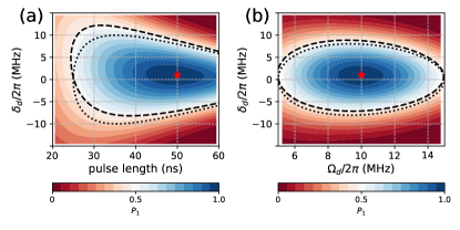
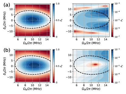
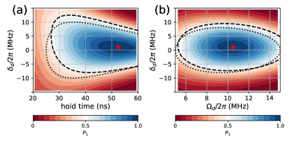
Generally, as shown in Fig. 1(c), by tuning the qubit on-resonance with the global drive, single-qubit X rotations can be achieved. However, we note that since the initial Bloch vector is slightly tilted, as shown in Fig. 1(b), a small drive detuning is needed for enabling ideal X rotations with respect to the initial Bloch vector defined by Eq. (3). Thus, according to Z control pulses, X rotations can be realized by tuning the qubit from the idle point to the working point with a small overshoot Barends2019 . This fact is further illustrated by the results shown in Fig. 2. By initializing the qubit in state and using square pulses (results with cosine-decorated square pulses can be found in Appendix A), Figure 2(a) shows populations , i.e., the population in state at the end of the applied pulse, versus the drive detuning and the pulse length. Here, the drive amplitude is and the detuning at the idle point is . Similarly, given a fixed pulse length of , Figure 2(b) shows versus and . The optimal parameters for X rotations are indicated by the red stars. Indeed, we find that a small frequency overshoot is needed for X rotations.
In the present work, note that choosing gates as the native gates could simplify the tune-up procedure of single-qubit gate operations. This is because:
(i) arbitrary single-qubit rotations can be generated by two gates and three Z gates McKay2017 , i.e., , with ;
(ii) compared with the native X gate, the implementation of gates does not pose stringent requirements on the on-resonance condition, i.e., even the qubit is slightly off-resonance with the drive, gates can still be achieved. This can be captured by the analytical expression of Rabi oscillations for the two-level system initialized in state , i.e., Rabi’s formula
| (5) |
From Eq. (5), implementing gates requires at the end of the applied pulse, giving rise to the relations among the pulse length, the drive detuning , and the drive amplitude , as illustrated by the dotted lines of Fig. 2. Accordingly, the results based on numerical simulations are also presented, as indicated by the dashed line of Fig. 2. Note here that the derivation of the analytical equation ignores the slight tilt at the idle point, and this explains the discrepancy between the analytical and numerical results. Both the analytical and numerical results show that compared to X rotations, the available parameter ranges of rotations can provide great flexibility in its tune-up procedure.
Generally, due to the flexibility of rotations, for tuning-up gates, the above-mentioned overshoot can be ignored. In the next subsection, we will show that following this way, given a fixed drive detuning, gates can be realized by only optimizing the ramp times of control pulses, as suggested by Fig. 2(a). Meanwhile, in large-scale quantum systems with multiplexed control, this flexibility can be the most encouraging advantage as to mitigate single-qubit gate error due to stray coupling between qubits and to compensate for the non-uniformity of qubit parameters. This will be discussed in detail in Sec. IV.
II.2 Baseband control of qubit with fast-adiabatic ramps
In the above discussion, the single-qubit baseband control is discussed for an ideal two-level system. Nevertheless, for practical superconducting qubits, such as the transmon qubit, the weak qubit anharmonicity makes single-qubit gate operations particularly prone to leakage outside the qubit subspace. For one such baseband control transmon qubit, which is driven by an always-on global drive, the system Hamiltonian is (hereafter, transmon qubits are modeled as anharmonic oscillators Koch2007 )
| (6) |
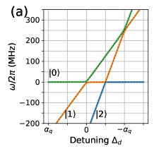
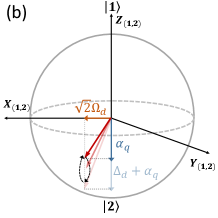
Here, is the annihilation (creation) operator. Figure 3(a) shows the energy spectrum of the driven qubit versus the drive detuning with qubit anharmonicity , drive frequency , and drive amplitude . One can find that due to the global drive, there exits an off-resonance coupling between states and , which can cause leakage to state when performing X rotations, i.e., biasing the qubit from its idle point to the working point. Note that there exist two leakage channels, caused by the and interactions, as shown in Fig. 3(a). Since the interaction involves second-order processes, generally, the induced leakage error is far smaller than that of the interaction. Here, we thus mainly focus on the leakage error caused by the interaction. However, we note that in our numerical analysis, all the leakage channels, including the interaction, are taken into consideration. While this leakage issue can be addressed by using the DRAG scheme in the traditional microwave control setup, this scheme cannot be directly utilized for the baseband flux control setup, as here only Z control is available.
Additionally, in principle, at the idle point, qubits could be far detuned above or below the frequency of the always-on drive. However, to avoid possible leakage error during qubit control, such as gate operations, qubit initialization, and readout, we prefer to bias the qubit away from the harmful avoid crossing caused by coupling between states and , as shown in Fig. 3(a). In this way, during the baseband-controlled gate operations, the qubit system will not sweep through or operate nearby this harmful avoid crossing, generally allowing the suppression of the leakage to state . Considering this fact, hereafter, we consider biasing the qubit below the drive frequency at the idle point. Even in the setting, during Z-controlled single-qubit gate operations, leakage error can still occur due to the non-adiabatic error, as shown in Fig. 3(b). In the following, we will consider using a fast-adiabatic control scheme for suppressing the leakage further.
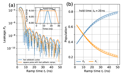
As shown in Fig. 3(b), the leakage error occurs when one non-adiabatically varies the driving detuning. Considering that coherence times of superconducting qubits are still limited, our target is to find a good flux control pulse, thus the non-adiabatic error is suppressed while maintaining a fast operation speed. Fortunately, this issue has already been addressed successfully by using a fast-adiabatic scheme introduced in Ref. Martinis2014b . Within the scheme, optimal control pulses can be obtained for minimizing non-adiabatic errors for any pulse longer than the chosen pulse length. However, we note that the original scheme only addresses the non-adiabatic error in the pulse ramps. Thus, here, to address the leakage issue in our setting, we consider using a square control pulse with optimal fast-adiabatic ramps, which is obtained following the fast-adiabatic scheme Martinis2014b (see Appendix B for details). The inset of Fig. 4(a) shows the optimal ramp pulse (solid blue line), which is used for generating our target control pulse with a flat middle part and fast-adiabatic ramps (solid orange line). Hereafter, we refer to this pulse as the fast-adiabatic flat-top pulse.
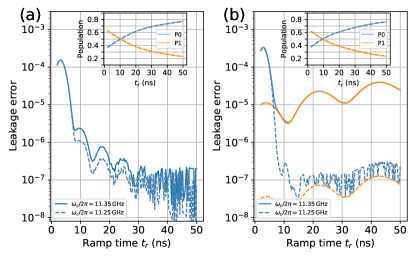
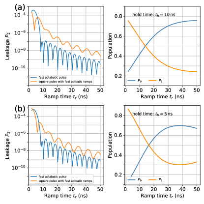
Here, we turn to evaluate the efficiency of the proposed fast-adiabatic flat-top pulse. We consider that the qubit idle frequency is and during the implementation of single-qubit X rotations, the drive detuning varies from the idle point at to the work point at and then coming back, according to the fast-adiabatic flat-top pulse. By initializing the qubit in state , Figure 4(a) shows the population leakage to state as a function of ramp times with the hold time of 20 ns and the qubit anharmonicities . For easy comparison, the results for applying only the fast-adiabatic pulse are also presented. One can find that by using the fast-adiabatic flat-top pulse, the leakage can be suppressed below for ramp times longer than 10 ns, and inserting a square pulse in the fast-adiabatic pulse does not change the efficiency of the original fast-adiabatic scheme. In Fig. 4(b), we also show the populations in and versus the ramp times. Additionally, Appendix B presents further results for different drive strengths.
From the results shown in Fig. 4, one can find that rotations can be realized with the ramp time at about 10 ns, giving rise to the total pulse length of about 30 ns. Meanwhile, same as the case for two-level systems (in Sec.II.1), here, single-qubit Z rotations can be easily implemented by controlling the time delay between Z pulses. Therefore, we could reasonably expect that with the help of the fast-adiabatic scheme, fast-speed single-qubit operations could be achieved with low leakage errors (we will evaluate the single-qubit gate performance in detail in the following section).
II.3 Dephasing due to fluctuations in the drive amplitude
Within the introduced baseband control setup, at the idle point, the global always-on drive acts as an off-resonance drive and can induce ac-Stark frequency shifts on the qubits. For the two-level system studied in Sec.II.1, the shift is given as , while, taking the higher energy levels of the transmon qubit into consideration, the shift is Schneider2018
| (7) |
From Eq. (7), the shift has a quadratic-dependent on the drive amplitude, making the qubit frequency more susceptible to possible amplitude noise. Therefore, fluctuations in the drive amplitude can cause qubit dephasing, which has been recently observed in superconducting qubits Wei2022 .
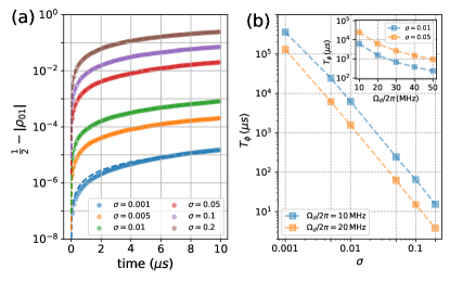
Here, to numerically study the amplitude-fluctuation-induced qubit dephasing, we consider an amplitude-dependent noise, i.e., amplitude fluctuations are proportional to the amplitudes. By assuming the drive subject to zero-mean Gaussian noise, i.e., , we numerically simulate the time evolution of the off-diagonal matrix element for the qubit initialized in state . After averaging over 2000 trajectories (i.e., realizations of noise), the magnitudes of the off-diagonal matrix element display a clear exponential decay, as shown in Fig. 5(a). Here, the evolution time is , the other used parameters are: , , and , giving rise to . By fitting the decay curves to , Figure 5(b) shows the dephasing time versus the noise variance . Here, we also show the results for . Additionally, in the inset, we further show the dephasing times versus the drive amplitudes.
From the results shown in Fig. 5(b), and given the typical noise variance of , we can conclude that the amplitude-noise induced dephasing can be safely neglected by detuning the qubit far from the drive frequency. Meanwhile, we note that to ensure high-fidelity gate operations within sub-100 ns, the drive amplitude itself should be larger than . Finally, we note that besides the qubit dephasing, when the always-on drive is shared by multiple qubits, there are two additional potential issues related to the drive and its fluctuation:
(i) qubit decoherence due to the excess quasiparticles (QPs) Catelani2011 . Previous works have demonstrated that QPs can be injected into a qubit by applying a high-power microwave pulse resonance with its readout resonator Vool2014 ; Wang2014 . However, at the present setting, the strength of the always-on drive is far smaller than that of the former case, we thus expect that the contribution of the always-on drive to the excess QPs is negligible.
(ii) when the always-on shared (global) drive is shared by multiple qubits, fluctuations in the drive can result in errors on multiple qubits. At first glance, this can cause correlated errors. However, as discussed in Ref. Fowler2014 , provided the fluctuation is small and quantum error correction is frequent, the fluctuation in the shared drive can result in a correlated probability of error on multiple qubits, but the errors themselves will not be correlated. Additionally, as suggested in Fig.5(b) and Eq.(7), by increasing the qubit-drive detuning, the fluctuation-induced dephasing (error) can be heavily suppressed at the system idle time. And during single-qubit gate operations, with the currently available control electronics, single-qubit gates with gate errors below 0.0001 have been demonstrated Somoroff2021 ; Li2023 . Thus, we argue that fluctuations in the shared drive itself can indeed cause errors, but probably a rather small one (). In this case, the control-noise-induced error may still be handled by the error correction schemes Fowler2014 .
II.4 Impact of the always-on drive on the qubit readout
As mentioned in Sec. I and Sec. II.1, due to the presence of the always-on drive, in this work, the microwave dressed states are defined as the computational states. Here, since the available control over the always-on drive is limited, the previous method Zhao2022 ; Huang2021 , in which the dressed state is first mapped back to the corresponding bare state, and then the traditional dispersive readout is employed for inferring the qubit information Wallraff2005 , cannot be directly utilized. However, as discussed in Sec. II.1, when the drive detuning is far larger than the drive amplitude, i.e., , the difference between dressed states and bare states can be neglected. Therefore, we expect that by keeping a large ratio of the drive detuning to the drive amplitude, the qubit information can be directly inferred using the traditional dispersive readout scheme.
To explore the possible impact of the always-on drive on the qubit dispersive readout, we numerically simulate the system dynamics during the dispersive readout. By applying a 250-ns square readout pulse with frequency and amplitude to the readout resonator with decay rate , the full system dynamics are governed by the Hamiltonian
| (8) | ||||
where denotes the qubit Hamiltonian given in Eq. (6), is the frequency of the readout resonator, is the annihilation (creation) operator of the resonator, and denotes the strength of the qubit-resonator coupling. In this following, the qubit information is encoded into single quadrature, i.e., -quadrature, by choosing the readout frequency to be Wallraff2005 . Here, and denote the dressed resonator frequencies with the qubit in states and , respectively. The other system parameters are: , , , , , , and .
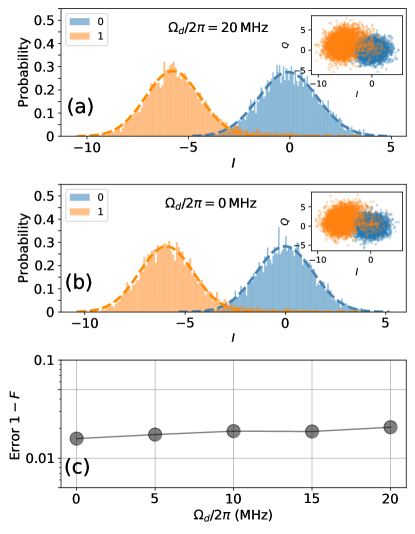
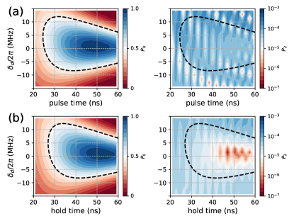
According to Eq. (8), we simulate the system dynamics based on solving the stochastic master equation Johansson2012 . Then, following Ref. Walter2017 , we further caulate the integrated readout quadrature with an optimal weight function (see Appendix C for details). With 5000 repetitions of the simulation for each qubit basis state, i.e., and , Figure 6(a) shows the two histograms of the integrated readout quadrature with the qubit prepared in states and , respectively. Here, the drive magnitude is . For easy comparison, we also present the result for the global drive is absent, as shown in Fig. 6(b).
Fitting the histograms to Gaussian functions gives the state-decision threshold at the intersection point of the two fitted distributions. Accordingly, the readout fidelity can be calculated as , where () denotes the error probability that the qubit initialized in state () is identified as in state (). Accordingly, Figure 6(c) shows the readout error versus the drive strength. One can find that when increasing the drive amplitude from to , while the error shows an upward trend, the increased error is below . Moreover, the upward trend also suggests that by further increasing the ratio , the increased error should be heavily suppressed.
III An Application in qubit architectures with tunable coupling
Given the overview of the baseband control scheme, in this section, we will present the application of this scheme in a qubit architecture with tunable coupling. As depicted in Fig. 1(a), we consider that two frequency-tunable transmon qubit and are coupled via a tunable coupler (i.e., an auxiliary transmon qubit) and both qubits are driven by an always-on global drive. After applying RWA, the system Hamiltonian is given by
| (9) | ||||
where and are the bare qubit frequency and the qubit anharmonicity of , is the associated annihilation (creation) operator, and denotes strength of the coupling between and . Hereafter, the system state is denoted by the notation and the used system parameters are: the qubit anharmonicity , the coupler anharmonicity , the direct qubit-qubit coupling strength (at ), the qubit-coupler coupling strength (at ), the drive amplitude , and the drive frequency .
Note here that the RWA is used for simplifying numerical simulation (otherwise, given the always-on drive, Floquet methods could be employed here Huang2021 ; Shirley1965 ; Sambe1973 ; Petrescu2021 ). However, in the present two-qubit system with tunable coupling, the non-RWA terms in the original Hamiltonian (see Appendix D for details) can significantly affect the effective coupling between qubits and can shift the bare qubit frequency. Thus, here, considering non-RWA terms while still working within the RWA formalism, we keep second-order corrections from the non-RWA terms and find that with this correction (details on its derivation can be found in Appendix D), the results agree well with the results without applying the RWA. Accordingly, the corrections are taken into consideration throughout the following discussion.
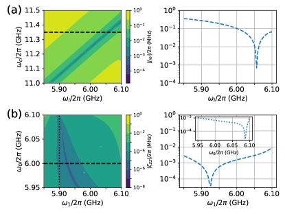
Before going into details of the baseband controlled gate operations, we give a few brief discussions of the tunable coupling architecture. For performing gate operations in multiqubit systems, the key benefit of the introduced tunable coupler is that the inter-qubit coupling strength can be tuned off by biasing the coupler at a certain frequency point, i.e., zero-coupling point. However, the zero-coupling point can change when the qubit is just biased slightly away from its idle point. Fortunately, in the tunable coupling architecture, biasing the qubit slightly away, generally, only causes a small increase in the residual inter-qubit coupling. This can be found in Fig. 7. Figure 7(a) shows the strengths of the residual resonance XY coupling versus the qubit frequency and the coupler frequency, while Figure 7(b) shows the residual ZZ coupling versus the frequencies of the two qubits with the coupler frequency fixed at . Here, the XY coupling and the ZZ coupling are numerically calculated by the diagonalization of the Hamiltonian Eq. (9) in the rotating frame defined by the always-on drive. To be more specific, the XY coupling is extracted as half the energy difference between dressed eigenstates and , while the ZZ coupling is . Here, denotes the energy of dressed eigenstate , which is adiabatically connected to the bare state Ghosh2013 .
According to the above results, in the following discussion, we consider that at the system idle point, the frequency of qubit and qubit are and , respectively, and the frequency of coupler is . Therefore, the residual ZZ coupling is below at the system idle point. Moreover, during the gate operations based on slightly tuning qubit frequency, such as implementing single-qubit gates by tuning the qubit from its idle point to the working point (e.g., at ), the residual inter-qubit ZZ coupling can always be below .
III.1 Single-qubit gate operation
Following the scheme introduced in Sec. II.2, here, Z-controlled single-qubit gates are realized by using the fast-adiabatic flat-top pulse. Note here that in the present two-qubit system, single-qubit gate operations for one qubit are tuned up and characterized with the other qubit in its ground state .
Figure 8 shows the leakage versus the ramp time of the pulse with the qubit initialized in its excited state . One can find that while for , the result is in line with our theory discussed in Sec. II.2, i.e., by increasing the ramp time, the leakage can be further suppressed, the result of seems unreasonable at first glance. However, during gate operations applied to , is tuned from its idle point at to the working point at about , according to the fast-adiabatic pulse, while is fixed at its idle point at . Therefore, during the pulse ramp, will sweep through a tiny avoided crossing formed by the residual resonance XY coupling between and at . On contrast, during single-qubit gate operations, will not sweep through . As shown in Fig. 7(a), the strength of the residual XY coupling is about . Thus, sweeping through this avoided crossing slowly will generally cause more leakage into the nearby qubit , as shown in Fig. 8(b), where the orange solid line denotes the population of in state . One can find that for , the leakage into gives the leading contributions to the total leakage error. These results suggest that there exists a trade-off between gate error resulting from the qubit itself and error from spectator qubits, i.e., suppressing leakage into favors longer gate times, while mitigating the leakage into the favors short gate times. This observation is in agreement with that in previous work Zhao2022b .
To address the above issue, one can change the idling coupler frequency, the XY coupling can thus be further suppressed at the resonance point, i.e., . By biasing the coupler at , the residual XY coupling is suppressed below . Accordingly, the leakage into is indeed suppressed heavily, as shown in Fig. 8(b), where the dashed lines show the results with the coupler biased at .
Here, we turn to evaluate the gate performance of the baseband controlled single-qubit gates, and use the metric of the state-average gate fidelity Pedersen2007 in the following discussion (details on the fidelity calculation can also be found in Ref. Zhao2022b ). As mentioned in Sec. II.1, in the present work, we focus on the implementation of gates. From the inset of Figs. 8(a) and 8(b), one can find that for both qubits, gates can be realized with a ramp time of about , giving rise to the total gate time of about . Moreover, even by biasing the coupler at , Figure 8 shows that when the ramp time is about , the leakage error can still be suppressed below for both qubits. This is to be expected, since sweeping through the tiny avoided crossing with fast speed could suppress leakage. By optimizing the ramp times, we find that for both qubits, up to single-qubit Z rotations, gates can be achieved with gate fidelity exceeding (for , the gate fidelity is and the optimal gate time is , while for , are the and ). As mentioned before, Z gates can be easily realized by choosing suitable time delays between flux pulses. In this way, universal single-qubit gates can be achieved by combining Z gates and gates.
III.2 Two-qubit CZ gate
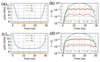
Having discussed the single-qubit control, we now turn to the two-qubit case. Here, we consider the implementation of CZ gates in the two-qubit system with an always-on drive. During the gate operations, is fixed at its idle point, i.e., , is tuned from its idle point () to the working point, where a complete oscillation between states and can occur. Meanwhile, the coupler is tuned from its idle point at to a working point at about , giving rise to the CZ coupling strength of (see Appendix D).
Figure 9(a) shows the typical control pulse, i.e., the pulse with a flat middle part and cosine-shaped ramps (see Appendix A for details), with a pulse length of for the CZ implementation. By numerically optimizing the working points of and , the gate fidelity of the implemented CZ gate (up to single-qubit Z phases) is . After inspecting the qubit dynamics during the gates, one can find that the leading error source is the population swap between two qubits, as shown in Fig. 9(b). Following the fast-adiabatic scheme discussed in Sec. II.2 and the previous work Martinis2014b ; Sung2021 , here, the fast-adiabatic flap-top pulses, as shown in Fig. 9(c), with a hold time of , is used to suppress the population swap. Accordingly, the population swap is indeed largely suppressed, as shown in Fig. 9(d), improving the CZ gate fidelity to with a gate time of . Additionally, we note that generally, by increasing the gate length, the residual gate error can be further suppressed (see also in Appendix E).
The above results show that although there exists an always-on global drive, high-fidelity two-qubit gates can still be achieved in a short time. This success is mainly based on the fact that during the gate operations, the global drive is far detuned from both qubits and the coupler.
IV discussion
Given the above theoretical analysis of the implementation of the baseband flux control in tunable coupling architecture, in the following, we will give a few discussions of the challenges and opportunities for realizing the baseband control strategy in large-scale superconducting quantum processors.
IV.1 Practical challenges
While our theoretical study shows that baseband controlled gate operations can be realized with high fidelity and fast speed, we note that besides the qubit decoherence, there exist several practical experimental issues that will limit the available gate performance:
(i) Flux pulse distortion. Flux pulse distortion has been demonstrated as a critical issue faced by baseband flux-controlled gate operations Jerger2019 ; Rol2020 ; Foxen2019 . Moreover, the above-demonstrated high-fidelity gate operations are achieved by using pulse shaping technologies, thus, the impact of flux pulse distortion can become more prominent in our setting.
(ii) Stray coupling beyond nearest neighbors. Generally, in our setting, the always-on drive is shared by multiple qubits. When performing single-qubit gates in parallel, multi-qubit will be tuned on-resonance with the same drive. This means that any stray coupling between these qubits will cause population swaps among these qubits, as discussed in Sec. III.1, leading to additional gate errors compared to isolated gates. While near-neighbor couplings between qubits can be controlled well in the tunable coupling architecture, parasitic coupling beyond nearest neighbors can still exist due to, such as stray capacitive coupling, in multi-qubit systems Barends2014 ; Zajac2021 ; Yanay2022 ; Zhao2022b . This will degrade the efficiency of the baseband control strategy in large-scale quantum processors.
(iii) Defect modes, such as TLSs Muller2019 . Same as in (ii), when performing single-qubit gates, the working frequencies of multi-qubit are almost limited to a fixed one, i.e., the frequency of the shared drive. This will limit the ability to mitigate the impacts from defect modes by tuning the qubit away from the defects Klimov2018 .
(iv) Keeping track of the single-qubit phase accumulation. In our setting, the qubit frequency at its idle point is detuned from the always-on drive. Thus, the single-qubit phase will accumulate at the speed of the drive detuning during the idle time. While the accumulated phase can be employed to realize single-qubit Z gates, on the other hand, when performing gate sequences or quantum circuits, the accumulated phase should be tracked carefully over the whole time domain. Compared with the traditional microwave control, this could complicate the implementation of quantum circuits.
In addition, we note that owing to the great flexibility of Z-controlled gates, as discussed in Sec.II.1, the issues, related to (ii) and (iii), may be addressed. From the results shown in Fig. 2, we can find that given a fixed drive amplitude or a fixed pulse length, gates can be achieved with a small drive detuning, for which its magnitude can even be compared with that of the always-on drive. Thus, when implementing isolated or paralleled single-qubit gates, the working frequencies of qubits can be biased intentionally at different frequency points, thus impacts of sub-MHz stray coupling can be mitigated. Similarly, the defect’s impact can be suppressed by biasing qubits away from the leading defect modes.
IV.2 Opportunities for solving challenges towards large-scale quantum processors
Currently, in small-scale superconducting quantum processors, each qubit has its dedicated control lines, such as XY lines and flux (Z) lines. Moreover, due to the non-uniformity of qubit parameters, such as qubit frequency and anharmonicity, the coupling efficiency between qubits and control lines, and the signal attenuation and the distortion in control lines, control pulses can differ from qubit to qubit. Thus, generally, microwave control pulses differ with each other in their amplitudes, frequencies, and phases, while for the baseband flux pulse, their amplitudes could be different. When scaling up to large-scale quantum computing, such strategy is not scalable.
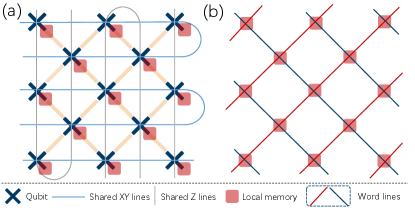
Given the recent progress in the pursuit of scalable spin-based quantum computing with multiplexing technologies and crossbar technologies Hill2015 ; Vandersypen2017 ; Veldhorst2017 ; Li2018 , we may also consider how to utilize these technologies for solving the above-mentioned challenges toward large-scale superconducting quantum processors. One possible example is schematically illustrated in Fig. 10(a), where both the XY and Z lines are shared by multiple qubits in a square lattice of frequency-tunable qubits. Similarly, in qubit architectures with tunable couplers, the Z-line shared scheme could be employed for controlling tunable couplers, thus enabling the implementation of baseband-controlled two-qubit gates in parallel.
Note that in principle, the shared control scheme should be applicable for driving all qubits with a single continuous microwave source. As a practical application, we expect that the shared scheme could be feasible for tens of superconducting qubits. With this strategy, the number of needed microwave drive lines is, at least, an order of magnitude less than that in the traditional setting. Additionally, to integrate with the widely used flip-chip technology, the shared drive may be applied to multiple qubits through a shared XY line. According to the discussion given in Ref. Krinner2019 , we estimate that when the strength of the always-on microwave drive is about 10 MHz ( gates with a gate time of 30 ns), the required power is about -14 dBm at the room temperature, and through a series of attenuators and filters (giving rise to the total attenuation of 60 dB), the actual power delivered to the qubit chip is about -74 dBm. As in the traditional setting, the average required power per qubit drive line is about -78 dBm (to the qubit chip) Krinner2019 , we expect that the heating issue of the present shared control scheme can be addressed.
Compared with the spin qubit, it seems that the superconducting qubit can provide more flexible control over its physical size and qubit parameters Martinis2020 ; Barends2014 ; Zhao2020N ; Mamin2022 ; Zhao2022c ; Chow2015 , yet, it can also show prominent non-uniformity. Unfortunately, the success of the multiplexing technologies and crossbar technologies highly hinges on the uniformity of qubit parameters. This can be more prominent for superconducting quantum processors based on individual microwave control. In the context of the implementation of multiplex control of superconducting qubits, baseband flux control may alleviate this issue of non-uniformity. Within our baseband control setup, and applying the multiplexing technologies shown in Fig. 10(a), there are three main leading challenges from the qubit non-uniformity:
(i) The non-uniform amplitude of the shared microwave drive or (ii) flux pulse felt by qubits (caused by, such as the different coupling efficiency between qubits and the global XY/Z line and the signal attenuation in control lines);
(iii) Independently calibrated parameters of flux pulse, including pulse length and pulse shape, for implementing accurate control on individual qubits.
However, as discussed in Sec.II.1, for two-level systems, given a fixed pulse length and pulse shape (i.e., square shape, see Appendix A for results with smooth pulses), owing to the flexibility of Z-controlled single-qubit gates (based on gates), the available parameter ranges (i.e., the drive amplitude and the drive detuning) can be explored for compensating the non-uniform of drive amplitude. This exciting feature is illustrated in Fig. 2(b). Furthermore, similar results can also be obtained for superconducting qubits, such as transmon qubits. Figures 11(a) and 11(b) present the results for transmon qubits with - square pulses and smooth pulses (i.e., cosine-decorated square pulse with a hold time of and a ramp time of ), respectively. Here, the qubit anharmonicity is and the other used parameters are same as in Fig. 2. In addition, we note that to achieve uniform control pulses, the Z gate scheme based on time-delay and the proposed fast-adiabatic scheme cannot be employed. Here, we can instead use cosine-decorated square pulses for implementing Z gates by tuning the qubit from the idle point, and for suppressing leakage. From Figs. 11(a) and 11(b), one can find that by adding cosine-shaped ramps, the leakage error can be suppressed below , while for the square pulse the leakage can approach . To further suppress the leakage error, one can increase the ramp time or decrease the drive amplitude. However, this will increase gate length and thus cause more decoherence errors.
Considering the above results, the above three challenges can be effectively overcome by only addressing the non-uniformity issue of flux pulse amplitudes. This non-uniformity issue could be removed by developing on-chip programmable memory, such as the one demonstrated by using Single Flux Quantum (SFQ) logic Johnson2010 ; McDermott2010 , which could be used to compensate for the remaining non-uniformity. In this way, combined with the word lines for digital addressing, as shown in Fig. 10(b), it is possible using only a few global XY and Z lines to achieve parallel control of large numbers of qubits Hill2015 ; Vandersypen2017 ; Veldhorst2017 ; Li2018 . Nevertheless, given the practical experimental limitations, such as the limited cooling power, the realization of the local programmable memory, which is compatible with superconducting qubits, is still rarely explored Johnson2010 , and undoubtedly, will be one of the most crucial challenges for implementing multiplexing control technologies. Last, but not least, we must stress that before solving the issue of pulse distortion, the efficiency of the above-discussed scheme could be limited for implementing gate-based quantum computing.
V conclusion
In this work, we propose and theoretically study the possibility of implementing baseband control of superconducting qubits, which are subjected to an always-on global drive. Our results provide a general understanding and the basic principles of realizing the baseband control scheme for superconducting qubits, such as frequency-tunable transmon qubits. In the qubit architecture with tunable coupling, we show that high-fidelity and fast-speed gate operations are possible by employing this baseband control scheme. Additionally, we have further discussed potential challenges and opportunities for implementing such baseband control strategy toward large-scale superconducting quantum processors.
Acknowledgements.
We acknowledge helpful discussions with Zhaohua Yang, Yanwu Gu, and Zhi-Hai Liu. This work was supported by the National Natural Science Foundation of China (Grants No.12204050, No.11890704, and No.11905100), the Beijing Natural Science Foundation (Grant No.Z190012), and the Key-Area Research and Development Program of Guang Dong Province (Grant No. 2018B030326001). P.X. was supported by the National Natural Science Foundation of China (Grant Nos. 12105146, 12175104).Note added.– During the preparation of this manuscript, we became aware of a recent related work Bejanin2022 , which presents the experimental demonstration of baseband-controlled single-qubit gates in superconducting transmon qubits.
Appendix A Flexibility of rotations
In Fig. 2, we show the dynamics of Z-controlled two-level systems subjected to an always-on drive. Here, as shown in Fig. 12, we further present the result for the case with cosine-decorated square pulses, i.e.,
| (10) |
where, denotes the peak pulse amplitude, is the ramp time, and represents the total pulse length. One can find that same as that with square pulses, to implement X rotations, a small overshoot is needed, as indicated by the red stars. Accordingly, as shown in Fig. 13, we also give the results, including both the population in state and the leakage into state , for the transmon qubit. Here the qubit anharmonicity is , and the transmon qubit is prepared in state .
Appendix B fast-adiabatic pulse
As discussed in the main text, the fast-adiabatic scheme is employed for designing an optimal control pulse for suppressing leakage Martinis2014b . Our strategy is using the Slepian-based method to design an optimal ramp pulse, and then inserting a square pulse into the optimal pulse. In this way, the target fast-adiabatic flat-top pulse is synthesized for implementing low-leakage X rotations. Therefore, here we only focus on finding the optimal ramp pulse. As shown in Fig. 3(a), the leakage error results from the non-adiabatic evolution in the leakage subspace. Generally, during X rotations i.e., the drive detuning varies from the idle point with the control angle to the working point with the control angle , and then comes back. Following Ref. Martinis2014b , the ramp pulse with a length of can be parameterized in terms of Fourier basis functions, and is given by
| (11) |
with constraints on the coefficients . Here, to find the optimal pulse, we consider keeping three Fourier terms. Following Ref. Martinis2014b , the three optimized coefficients can be obtained numerically by minimizing the integrated spectral density of the pulse above a chosen frequency.
In the main text, the efficiency of the above-discussed optimal pulse is only evaluated with the drive amplitude of . Here, we present more results with different drive strengths. In Figs. 14(a) and 14(b), we show the results with and , respectively. Similar to the results shown in Fig. 4, we find that fast-speed rotations can be realized with low leakage.
Appendix C readout
Here for easy reference, following Ref. Walter2017 , we briefly describe the processing of the recording obtained from continuous measurement to infer qubit states. As mentioned in the main text, by encoding the qubit information into single quadrature, i.e., in-phase quadrature , the qubit state can be inferred by recoding during the continuous measurement. To maximize the readout fidelity with a given measurement time (here is ), the records of are integrated over the measurement time with a weight function, giving rise to the integrated readout quadrature value
| (12) |
with the weight function
| (13) |
Here, and represent the expectation values of for the qubit prepared in and , respectively.
Appendix D RWA and corrections
For two frequency-tunable transmon qubits ( and ) coupled via a tunable coupler , the system Hamiltonian is given by
| (14) | ||||
After applying the RWA, the non-RWA term, i.e., the terms in the third line of Eq. (14), is omitted, giving rise to
| (15) | ||||
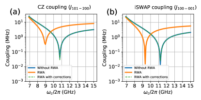
As mentioned in the main text, the non-RWA term can significantly affect the effective coupling between qubits and shift the bare qubit frequency. This can be found in Fig. 15, where the numerically calculated XY coupling strengths for iSWAP coupling (the resonance coupling between and ) and CZ coupling (the resonance coupling between and ) are presented based on Eq. (14) and Eq. (15).
To remove the discrepancy within the RWA formalism, we consider eliminating the non-RWA terms in Eq. (14) by using the unitary transformation Zueco2009 ; Yan2018
| (16) |
with . This gives . Expanding the above equation and keeping term up to second-order in the small parameters , we have
| (17) | ||||
with the renormalized qubit frequency and coupler frequency
| (18) | ||||
and the effective strength of qubit-qubit coupling
| (19) |
Taking the above-obtained corrections into consideration, the results (dashed lines) with the RWA show a great agreement with the results without the RWA, as shown in Fig. 15. Finally, we note that in our numerical analysis, each transmon qubit is modeled as an anharmonic oscillator truncated with five levels. Additionally, to further reduce the computational expenses, we further project the full system Hamiltonian to a smaller subspace where at most five excitations are permitted. We justify this choice by checking the resulting gate error compared to models with more energy levels or excitations and find that the variation of the gate error is below .
Appendix E CZ gate error
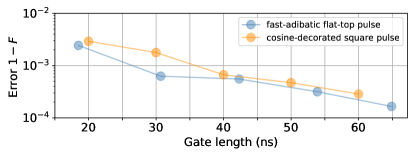
As mentioned in the main text, generally, increasing the gate length can further suppress the parasitic interaction (i.e., qubit-qubit swap interactions and qubit-coupler swap interactions) induced gate errors. Here, we provide more numerical results on this issue. Figure 16 shows the gate error versus gate length for the discussed two types of pulses, i.e., the fast-adiabatic flat-top pulse and the cosine-decorated square pulse.
References
- (1) M. Kjaergaard, M. E. Schwartz, J. Braumüller, P. Krantz, J. I.-J. Wang, S. Gustavsson, and W. D. Oliver, Superconducting qubits: Current state of play, Annu. Rev. Condens. Matter Phys. 11, 369 (2020).
- (2) P. Krantz, M. Kjaergaard, F. Yan, T. P. Orlando, S. Gustavsson, and W. D. Oliver, A Quantum Engineer’s Guide to Superconducting Qubits, Appl. Phys. Rev. 6, 021318 (2019).
- (3) F. Arute, K. Arya, R. Babbush, D. Bacon, J. C. Bardin, R. Barends, R. Biswas, S. Boixo, F. G. Brandao, D. A. Buell et al., Quantum supremacy using a programmable superconducting processor, Nature 574, 505 (2019).
- (4) Q. Zhu, S. Cao, F. Chen, M.-C. Chen, X. Chen, T.-H. Chung, H. Deng, Y. Du, D. Fan, M. Gong et al., Quantum Computational Advantage via 60-Qubit 24-Cycle Random Circuit Sampling, Sci. Bull. 67, 240 (2022).
- (5) Q. Acharya, I. Aleiner, R. Allen, T. I. Andersen, M. Ansmann, F. Arute, K. Arya, A. Asfaw, J. Atalaya, R. Babbush et al., Suppressing quantum errors by scaling a surface code logical qubit, arXiv:2207.06431.
- (6) Y. Kim, C. J. Wood, T. J. Yoder, S. T. Merkel, J. M. Gambetta, K. Temme, and A. Kandala, Scalable error mitigation for noisy quantum circuits produces competitive expectation values, arXiv:2108.09197.
- (7) A. G. Fowler, M. Mariantoni, J. M. Martinis, and A. N. Cleland, Surface codes: Towards practical large-scale quantum computation, Phys. Rev. A 86, 032324 (2012).
- (8) A. Gidney and M. Ekerå, How to factor 2048 bit RSA integers in 8 hours using 20 million noisy qubits, Quantum 5, 433 (2021).
- (9) D. P. Frankea, J. S. Clarkeb, L. M. K. Vandersypenab, and M. Veldhorsta, Rent’s rule and extensibility in quantum computing, Microprocess. Microsy. 67, 1 (2019).
- (10) D. J. Reilly, Challenges in Scaling-up the Control Interface of a Quantum Computer, 2019 IEEE International Electron Devices Meeting (IEDM), 31.7 (2019).
- (11) J. M. Martinis, Information Constraints for Scalable Control in a Quantum Computer, arXiv:2012.14270.
- (12) J. B. Hertzberg, E. J. Zhang, S. Rosenblatt, E. Magesan, J. A. Smolin, J.-B. Yau, V. P. Adiga, M. Sandberg, M. Brink, Je. M. Chow, and J. S. Orcutt, Laser-annealing Josephson junctions for yielding scaled-up superconducting quantum processors, npj Quantum Inf. 7, 129 (2021).
- (13) J. M. Kreikebaum, K. P. O’Brien, A. Morvan, and I. Siddiqi, Improving wafer-scale Josephson junction resistance variation in superconducting quantum coherent circuits, Supercond. Sci. Technol. 33, 06LT02 (2020).
- (14) J. Kelly, P. O’Malley, M. Neeley, H. Neven, and J. M. Martinis, Physical qubit calibration on a directed acyclic graph, arXiv:1803.03226.
- (15) P. V. Klimov, J. Kelly, J. M. Martinis, and H. Neven, The snake optimizer for learning quantum processor control parameters, arXiv:2006.04594.
- (16) Z. Chen, Metrology of Quantum Control and Measurement in Superconducting Qubits, Ph.D. thesis. University of California, Santa Barbara, 2018.
- (17) S. Krinner, S. Storz, P. Kurpiers, P. Magnard, J. Heinsoo, R. Keller, J. Lütolf, C. Eichler, and A. Wallraff,, Engineering cryogenic setups for 100-qubit scale superconducting circuit systems, EPJ Quantum Technology 6, 2 (2019).
- (18) J. Wenner, M. Neeley, R. C. Bialczak, M. Lenander, E. Lucero, A. D. ÓConnell, D. Sank, H. Wang, M. Weides, A. N. Cleland, and J. M. Martinis, Wirebond cross talk and cavity modes in large chip mounts for superconducting qubits, Supercond. Sci. Technol. 24, 065001 (2011).
- (19) D. Rosenberg, S. Weber, D. Conway, D. Yost, J. Mallek, G. Calusine, R. Das, D. Kim, M. Schwartz, W. Woods, J. L. Yoder, and W. D. Oliver, 3D integration and packaging for solid-state qubits, arXiv:1906.11146.
- (20) S. Huang, B. Lienhard, G. Calusine, A. Vepsäläinen, J. Braumüller, D. K. Kim, A. J. Melville, B. M. Niedzielski, J. L. Yoder, B. Kannan, T. P. Orlando, S. Gustavsson, and W. D. Oliver, Microwave Package Design for Superconducting Quantum Processors, PRX Quantum 2, 020306 (2021).
- (21) C. D. Hill, E Peretz, S J. Hile, M. G. House, M. Fuechsle, S Rogge, M. Y. Simmons, and L. C. L. Hollenberg, A surface code quantum computer in silicon, Sci. Adv. 1, e1500707 (2015).
- (22) L. M. K. Vandersypen, H. Bluhm, J. S. Clarke, A. S. Dzurak, R. Ishihara, A. Morello, D. J. Reilly, L. R. Schreiber, and M. Veldhorst, Interfacing spin qubits in quantum dots and donors-hot, dense, and coherent, npj Quantum Inf. 3, 34 (2017).
- (23) M. Veldhorst, H. G. J. Eenink, C. H. Yang, and A. S. Dzurak, Silicon CMOS architecture for a spin-based quantum computer, Nat. Commun. 8, 1766 (2017).
- (24) R. Li, L. Petit, D. P. Franke, J. P. Dehollain, J. Helsen, M. Steudtner, N. K. Thomas, Z. R. Yoscovits, K. J. Singh, and S. Wehner et al., A Crossbar Network for Silicon Quantum Dot Qubits, Sci. Adv. 4, eaar3960 (2018).
- (25) F. Motzoi, J. M. Gambetta, P. Rebentrost, and F. K. Wilhelm, Simple Pulses for Elimination of Leakage in Weakly Nonlinear Qubits, Phys. Rev. Lett. 103, 110501 (2009).
- (26) Z. Chen, J. Kelly, C. Quintana, R. Barends, B. Campbell, Y. Chen, B. Chiaro, A. Dunsworth, A. G. Fowler, E. Lucero, E. Jeffrey, A. Megrant, J. Mutus, M. Neeley, C. Neill, P. J. J. ÓMalley, P. Roushan, D. Sank, A. Vainsencher, J. Wenner, T. C. White, A. N. Korotkov, and J. M. Martinis, Measuring and Suppressing Quantum State Leakage in a Superconducting Qubit, Phys. Rev. Lett. 116, 020501 (2016).
- (27) J. M. Chow, A. D. Córcoles, J. M. Gambetta, C. Rigetti, B. R. Johnson, J. A. Smolin, J. R. Rozen, G. A. Keefe, M. B. Rothwell, M. B. Ketchen, and M. Steffen, Simple All-Microwave Entangling Gate for Fixed-Frequency Superconducting Qubits, Phys. Rev. Lett. 107, 080502 (2011).
- (28) D. L. Campbell, Y.-P. Shim, B. Kannan, R. Winik, D. K. Kim, A. Melville, B. M. Niedzielski, J. L. Yoder, C. Tahan, S. Gustavsson, and W. D. Oliver, Universal Nonadiabatic Control of Small-Gap Superconducting Qubits, Phys. Rev. X 10, 041051 (2020).
- (29) H. Zhang, S. Chakram, T. Roy, N. Earnest, Y. Lu, Z. Huang, D. K. Weiss, J. Koch, and D. I. Schuster, Universal Fast-Flux Control of a Coherent, Low-Frequency Qubit, Phys. Rev. X 11, 011010 (2021).
- (30) J. Koch, T. M. Yu, J. Gambetta, A. A. Houck, D. I. Schuster, J. Majer, A. Blais, M. H. Devoret, S. M. Girvin, and R. J. Schoelkopf, Charge-insensitive qubit design derived from the cooper pair box, Phys. Rev. A 76, 042319 (2007).
- (31) B. E. Kane, A silicon-based nuclear spin quantum computer, Nature (London) 393, 133 (1998).
- (32) G. Wolfowicz, M. Urdampilleta, M. L. W. Thewalt, H. Riemann, N. V. Abrosimov, P. Becker, H.-J. Pohl, and J. J. L. Morton, Conditional Control of Donor Nuclear Spins in Silicon Using Stark Shifts, Phys. Rev. Lett. 113, 157601 (2014).
- (33) A. Laucht, J. T. Muhonen, F. A. Mohiyaddin, R. Kalra, J. P. Dehollain, S. Freer, F. E. Hudson, M. Veldhorst, R. Rahman, G. Klimeck, K. M. Itoh, D. N. Jamieson, J. C. McCallum, A. S. Dzurak, and A. Morello, Electrically controlling single-spin qubits in a continuous microwave field, Sci. Adv. 1, e1500022 (2015).
- (34) Y.-x. Liu, C. P. Sun, and F. Nori, Scalable superconducting qubit circuits using dressed states, Phys. Rev. A 74, 052321 (2006).
- (35) P. Zhao, T. Ma, Y. Jin, and H. Yu, Combating fluctuations in relaxation times of fixed-frequency transmon qubits with microwave-dressed states, Phys. Rev. A 105, 062605 (2022).
- (36) K. X. Wei, E. Magesan, I. Lauer, S. Srinivasan, D. F. Bogorin, S. Carnevale, G. A. Keefe, Y. Kim, D. Klaus, W. Landers, N. Sundaresan, C. Wang, E. J. Zhang, M. Steffen, O. E. Dial, D. C. McKay, and A. Kandala, Hamiltonian Engineering with Multicolor Drives for Fast Entangling Gates and Quantum Crosstalk Cancellation, Phys. Rev. Lett. 129, 060501 (2022).
- (37) F. Yan, P. Krantz, Y. Sung, M. Kjaergaard, D. L. Campbell, T. P. Orlando, S. Gustavsson, and W. D. Oliver, Tunable Coupling Scheme for Implementing High-Fidelity Two-Qubit Gates, Phys. Rev. Appl. 10, 054062 (2018).
- (38) J. Tuorila, M. Silveri, M. Sillanpää, E. Thuneberg, Y. Makhlin, and P. Hakonen, Stark Effect and Generalized Bloch-Siegert Shift in a Strongly Driven Two-Level System, Phys. Rev. Lett. 105, 257003 (2010).
- (39) A. Schneider, J. Braumüller, L. Guo, P. Stehle, H. Rotzinger, M. Marthaler, A. V. Ustinov, and M. Weides, Local sensing with the multilevel ac stark effect, Phys. Rev. A 97, 062334 (2018).
- (40) J. M. Martinis and M. R. Geller, Fast adiabatic qubit gates using only control, Phys. Rev. A 90, 022307 (2014).
- (41) D. C. McKay, C. J. Wood, S. Sheldon, J. M. Chow, and J. M. Gambetta, Efficient z gates for quantum computing, Phys. Rev. A 96, 022330 (2017).
- (42) R. Barends, C. M. Quintana, A. G. Petukhov, Y. Chen, D. Kafri, K. Kechedzhi et al., Diabatic Gates for Frequency-Tunable Superconducting Qubits, Phys. Rev. Lett. 123, 210501 (2019).
- (43) G. Catelani, R. J. Schoelkopf, M. H. Devoret, and L. I. Glazman, Relaxation and frequency shifts induced by quasiparticles in superconducting qubits, Phys. Rev. B 84, 064517 (2011).
- (44) U. Vool, I. M. Pop, K. Sliwa, B. Abdo, C. Wang, T. Brecht, Y. Y. Gao, S. Shankar, M. Hatridge, G. Catelani, M. Mirrahimi, L. Frunzio, R. J. Schoelkopf, L. I. Glazman, and M. H. Devoret, Non-Poissonian Quantum Jumps of a Fluxonium Qubit due to Quasiparticle Excitations, Phys. Rev. Lett. 113, 247001 (2014).
- (45) C. Wang, Y.Y. Gao, I.M. Pop, U. Vool, C. Axline, T. Brecht, R.W. Heeres, L. Frunzio, M.H. Devoret, G. Catelani, L.I. Glazman, and R.J. Schoelkopf, Measurement and control of quasiparticle dynamics in a superconducting qubit, Nat. Commun. 5, 5836 (2014).
- (46) A. G. Fowler and J. M. Martinis, Quantifying the effects of local many-qubit errors and nonlocal two-qubit errors on the surface code, Phys. Rev. A 89, 032316 (2014).
- (47) A. Somoroff, Q. Ficheux, R. A. Mencia, H. Xiong, R. V. Kuzmin, and V. E. Manucharyan, Millisecond coherence in a superconducting qubit, arXiv:2103.08578.
- (48) Zhiyuan Li, Pei Liu, Peng Zhao, Zhenyu Mi, Huikai Xu, Xuehui Liang, Tang Su, Weijie Sun, Guangming Xue, Jing-Ning Zhang, Weiyang Liu, Yirong Jin, Haifeng Yu, Error per single-qubit gate below in a superconducting qubit, arXiv:2302.08690.
- (49) Z. Huang, P. S. Mundada, A. Gyenis, D. I. Schuster, A. A. Houck, and J. Koch, Engineering Dynamical Sweet Spots to Protect Qubits from Noise, Phys. Rev. Appl. 15, 034065 (2021).
- (50) A. Wallraff, D. I. Schuster, A. Blais, L. Frunzio, J. Majer, M. H. Devoret, S. M. Girvin, and R. J. Schoelkopf, Approaching Unit Visibility for Control of a Superconducting Qubit with Dispersive Readout, Phys. Rev. Lett. 95, 060501 (2005).
- (51) T. Walter, P. Kurpiers, S. Gasparinetti, P. Magnard, A. Potočnik, Y. Salathé, M. Pechal, M. Mondal, M. Oppliger, C. Eichler, and A. Wallraff, Rapid High-Fidelity Single-Shot Dispersive Readout of Superconducting Qubits, Phys. Rev. Applied 7, 054020 (2017).
- (52) J. Johansson, P. Nation, and F. Nori, QuTiP: An open-source Python framework for the dynamics of open quantum systems , Comput. Phys. Commun. 183, 1760 (2012).
- (53) J. H. Shirley, Solution of the Schrödinger Equation with a Hamiltonian Periodic in Time , Phys. Rev. 138, B979 (1965).
- (54) H. Sambe, Steady States and Quasienergies of a Quantum-Mechanical System in an Oscillating Field, Phys. Rev. A 7, 2203 (1973).
- (55) A. Petrescu, C. L. Calonnec, C. Leroux, A. D. Paolo, P. Mundada, S. Sussman, A. Vrajitoarea, A. A. Houck, and A. Blais, Accurate methods for the analysis of strong-drive effects in parametric gates, arXiv:2107.02343.
- (56) J. Ghosh, A. Galiautdinov, Z. Zhou, A. N. Korotkov, J. M. Martinis, and M. R. Geller, High-fidelity controlled- gate for resonator-based superconducting quantum computers, Phys. Rev. A 87, 022309 (2013).
- (57) P. Zhao, K. Linghu, Z. Li, P. Xu, R. Wang, G. Xue, Y. Jin, and H. Yu, Quantum Crosstalk Analysis for Simultaneous Gate Operations on Superconducting Qubits, PRX Quantum 3, 020301 (2022).
- (58) L. H. Pedersen, N. M. Møller, and K. Mølmer, Fidelity of quantum operations, Phys. Lett. A 367, 47 (2007).
- (59) Y. Sung, L. Ding, J. Braumüller, A. Vepsäläinen, B. Kannan, M. Kjaergaard, A. Greene, G. O. Samach, C. McNally, D. Kim, A. Melville, B. M. Niedzielski, M. E. Schwartz, J. L. Yoder, T. P. Orlando, S. Gustavsson, and W. D. Oliver, Realization of High-Fidelity CZ and ZZ-Free iSWAP Gates with a Tunable Coupler, Phys. Rev. X 11, 021058 (2021).
- (60) M. Jerger, A. Kulikov, Z. Vasselin, and A. Fedorov, In Situ Characterization of Qubit Control Lines: A Qubit as a Vector Network Analyzer, Phys. Rev. Lett. 123, 150501 (2019).
- (61) M. A. Rol, L. Ciorciaro, F. K. Malinowski, B. M. Tarasinski, R. E. Sagastizabal, C. C. Bultink, Y. Salathe, N. Haandbaek, J. Sedivy, and L. DiCarlo, Time-domain characterization and correction of on-chip distortion of control pulses in a quantum processor, Appl. Phys. Lett. 116, 054001 (2020).
- (62) B. Foxen, J. Y. Mutus, E. Lucero, E. Jeffrey, D. Sank, R. Barends, K. Arya, B. Burkett, Y. Chen, Z. Chen, B. Chiaro, A. Dunsworth, A. Fowler, C. Gidney, M. Giustina et al., High speed flux sampling for tunable superconducting qubits with an embedded cryogenic transducer, Supercond. Sci. Technol. 21, 015012 (2019).
- (63) R. Barends, J. Kelly, A. Megrant, A. Veitia, D. Sank, E. Jeffrey, T. C. White, J. Mutus, A. G. Fowler, B. Campbell, Y. Chen, Z. Chen, B. Chiaro, A. Dunsworth, C. Neill, P. O’Malley, P. Roushan, A. Vainsencher, J. Wenner, A. N. Korotkov, A. N. Cleland, and J. M. Martinis, Superconducting quantum circuits at the surface code threshold for fault tolerance, Nature 508, 500 (2014).
- (64) D. M. Zajac, J. Stehlik, D. L. Underwood, T. Phung, J. Blair, S. Carnevale, D. Klaus, G. A. Keefe, A. Carniol, M. Kumph, M. Steffen, O. E. Dial, Spectator Errors in Tunable Coupling Architectures, arXiv:2108.11221.
- (65) Y. Yanay, J. Braumüller, T. P. Orlando, S. Gustavsson, C. Tahan, and W. D. Oliver, Mediated Interactions beyond the Nearest Neighbor in an Array of Superconducting Qubits, Phys. Rev. Appl. 17, 034060 (2022).
- (66) C. Müller, J. H. Cole, and J. Lisenfeld, Towards understanding two-level-systems in amorphous solids: insights from quantum circuits, Rep. Prog. Phys. 82, 124501 (2019).
- (67) P. V. Klimov, J. Kelly, Z. Chen, M. Neeley, A. Megrant, B. Burkett, R. Barends, K. Arya, B. Chiaro, Y. Chen et al., Fluctuations of Energy-Relaxation Times in Superconducting Qubits, Phys. Rev. Lett. 121, 090502 (2018).
- (68) J. M. Chow, S. J. Srinivasan, E. Magesan, A. D. Córcoles, D. W. Abraham, J. M. Gambetta, and M. Steffen, Characterizing a four-qubit planar lattice for arbitrary error detection, Proc. SPIE 9500, Quantum Inf. Comput. 13, 95001G (2015).
- (69) R. Zhao, S. Park, T. Zhao, M. Bal, C. R. H. McRae, J. Long, and D. P. Pappas, Merged-Element Transmon , Phys. Rev. Appl. 14, 064006 (2020).
- (70) H. J. Mamin, E. Huang, S. Carnevale, C. T. Rettner, N. Arellano, M. H. Sherwood, C. Kurter, B. Trimm, M. Sandberg, R. M. Shelby, M. A. Mueed, B. A. Madon, A. Pushp, M. Steffen, and D. Rugar, Merged-Element Transmons: Design and Qubit Performance, Phys. Rev. Appl. 16, 024023 (2021).
- (71) P. Zhao, Y. Zhang, G. Xue, Y. Jin, and H. Yu, Tunable coupling of widely separated superconducting qubits: A possible application toward a modular quantum device, Appl. Phys. Lett. 121, 032601 (2022).
- (72) M. W. Johnson, P. Bunyk, F. Maibaum, E. Tolkacheva, A. J. Berkley, E. M. Chapple, R. Harris, J. Johansson, T. Lanting, and I. Perminov et al., A Scalable Control System for a Superconducting Adiabatic Quantum Optimization Processor, Supercond. Sci. Technol. 23, 065004 (2010).
- (73) R. McDermott, M. G. Vavilov, B. L. T. Plourde, F. K. Wilhelm, P. J. Liebermann, O. A. Mukhanov, and T. A. Ohki, Quantum-classical interface based on single flux quantum digital logic,Quantum Sci. Technol. 3, 024004 (2018).
- (74) J. H. Béjanin, C. T. Earnest, and M. Mariantoni, The Quantum Socket and DemuXYZ-Based Gates with Superconducting Qubits, arXiv:2211.00143.
- (75) D. Zueco, G. M. Reuther, S. Kohler, and P. Hänggi, Qubit-oscillator dynamics in the dispersive regime: Analytical theory beyond the rotating-wave approximation, Local sensing with the multilevel ac stark effect, Phys. Rev. A 80, 033846 (2009).