Basil: A Fast and Byzantine-Resilient Approach for Decentralized Training
Abstract
Decentralized (i.e., serverless) training across edge nodes can suffer substantially from potential Byzantine nodes that can degrade the training performance. However, detection and mitigation of Byzantine behaviors in a decentralized learning setting is a daunting task, especially when the data distribution at the users is heterogeneous. As our main contribution, we propose Basil, a fast and computationally efficient Byzantine-robust algorithm for decentralized training systems, which leverages a novel sequential, memory-assisted and performance-based criteria for training over a logical ring while filtering the Byzantine users. In the IID dataset setting, we provide the theoretical convergence guarantees of Basil, demonstrating its linear convergence rate. Furthermore, for the IID setting, we experimentally demonstrate that Basil is robust to various Byzantine attacks, including the strong Hidden attack, while providing up to absolute higher test accuracy over the state-of-the-art Byzantine-resilient decentralized learning approach. Additionally, we generalize Basil to the non-IID setting by proposing Anonymous Cyclic Data Sharing (ACDS), a technique that allows each node to anonymously share a random fraction of its local non-sensitive dataset (e.g., landmarks images) with all other nodes. Finally, to reduce the overall latency of Basil resulting from its sequential implementation over the logical ring, we propose Basil+ that enables Byzantine-robust parallel training across groups of logical rings, and at the same time, it retains the performance gains of Basil due to sequential training within each group. Furthermore, we experimentally demonstrate the scalability gains of Basil+ through different sets of experiments.
Index Terms:
decentralized training, federated learning, Byzantine-robustness.I Introduction
Thanks to the large amounts of data generated on and held by the edge devices, machine learning (ML) applications can achieve significant performance [1, 2]. However, privacy concerns and regulations [3] make it extremely difficult to pool clients’ datasets for a centralized ML training procedure. As a result, distributed machine learning methods are gaining a surge of recent interests. The key underlying goal in distributed machine learning at the edge is to learn a global model using the data stored across the edge devices.
Federated learning (FL) has emerged as a promising framework [4] for distributed machine learning. In federated learning, the training process is facilitated by a central server. In an FL architecture, the task of training is federated among the clients themselves. Specifically, each participating client trains a local model based on its own (private) training dataset and shares only the trained local model with the central entity, which appropriately aggregates the clients’ local models. While the existence of the parameter server in FL is advantageous for orchestrating the training process, it brings new security and efficiency drawbacks [5, 4]. Particularly, the parameter server in FL is a single point of failure, as the entire learning process could fail when the server crashes or gets hacked. Additionally, the parameter server can become a performance bottleneck itself due to the large number of the mobile devices that need to be handled simultaneously.
Training using a decentralized setup is another approach for distributed machine learning without having to rely on a central coordinator (e.g., parameter server), thus avoiding the aforementioned limitations of FL. Instead, it only requires on-device computations on the edge nodes and peer-to-peer communications. In fact, many decentralized training algorithms have been proposed for the decentralized training setup. In particular, a class of gossip-based algorithms over random graphs has been proposed, e.g., [6, 7, 8], in which all the nodes participate in each training round. During training, each node maintains a local model and communicates with others over a graph-based decentralized network. More specifically, every node updates its local model using its local dataset, as well as the models received from the nodes in its neighborhood. For example, a simple aggregation rule at each node is to average the locally updated model with the models from the neighboring nodes. Thus, each node performs both model training and model aggregation.
Although decentralized training provides many benefits, its decentralized nature makes it vulnerable to performance degradation due to system failures, malicious nodes, and data heterogeneity [4]. Specifically, one of the key challenges in decentralized training is the presence of different threats that can alter the learning process, such as the software/hardware errors and adversarial attacks. Particularly, some clients can become faulty due to software bugs, hardware components which may behave arbitrarily, or even get hacked during training, sending arbitrary or malicious values to other clients, thus severely degrading the overall convergence performance. Such faults, where client nodes arbitrarily deviate from the agreed-upon protocol, are called Byzantine faults [9]. To mitigate Byzantine nodes in a graph-based decentralized setup where nodes are randomly connected to each other, some Byzantine-robust optimization algorithms have been introduced recently, e.g., [10, 11]. In these algorithms, each node combines the set of models received from its neighbors by using robust aggregation rules, to ensure that the training is not impacted by the Byzantine nodes. However, to the best of our knowledge, none of these algorithms have considered the scenario when the data distribution at the nodes is heterogeneous. Data heterogeneity makes the detection of Byzantine nodes a daunting task, since it becomes unclear whether the model drift can be attributed to a Byzantine node, or to the very heterogeneous nature of the data. Even in the absence of Byzantine nodes, data heterogeneity can degrade the convergence rate [4].
The limited computation and communication resources of edge devices (e.g., IoT devices) are another important consideration in the decentralized training setting. In fact, the resources at the edge devices are considered as a critical bottleneck for performing distributed training for large models [4, 1]. In prior Byzantine-robust decentralized algorithms (e.g., [10, 11]), which are based on parallel training over a random graph, all nodes need to be always active and perform training during the entire training process. Therefore, they might not be suitable for the resource constrained edge devices, as the parallel training nature of their algorithms requires them to be perpetually active which could drain their resources. In contrast to parallel training over a random graph, our work takes the view that sequential training over a logical ring is better suited for decentralized training in resource constrained edge setting. Specifically, sequential training over a logical ring allows each node to become active and perform model training only when it receives the model from its counterclockwise neighbor. Since nodes need not be active during the whole training time, the sequential training nature makes it suitable for IoT devices with limited computational resources.
I-A Contributions
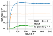
To overcome the aforementioned limitations of prior graph-based Byzantine-robust algorithms, we propose Basil, an efficient Byzantine mitigation algorithm, that achieves Byzantine robustness in a decentralized setting by leveraging the sequential training over a logical ring. To highlight some of the benefits of Basil, Fig. 1(a) illustrates a sample result that demonstrates the performance gains and the cost reduction compared to the state-of-the-art Byzantine-robust algorithm UBAR that leverages the parallel training over a graph-based setting. We observe that Basil retains a higher accuracy than UBAR with an absolute value of . Additionally, we note that while UBAR achieves its highest accuracy in rounds, Basil achieves UBAR’s highest accuracy in just rounds. This implies that for achieving UBAR’s highest accuracy, each client in Basil uses lesser computation and communication resources compared to that in UBAR confirming the gain attained from the sequential training nature of Basil.
In the following, we further highlight the key aspects and performance gains of Basil:
-
•
In Basil, the defense technique to filter out Byzantine nodes is a performance-based strategy, wherein each node evaluates a received set of models from its counterclockwise neighbors by using its own local dataset to select the best candidate.
-
•
We theoretically show that Basil for convex loss functions in the IID data setting has a linear convergence rate with respect to the product of the number of benign nodes and the total number of training rounds over the ring. Thus, our theoretical result demonstrates scalable performance for Basil with respect to the number of nodes.
-
•
We empirically demonstrate the superior performance of Basil compared to UBAR, the state-of-the-art Byzantine-resilient decentralized learning algorithm over graph, under different Byzantine attacks in the IID setting. Additionally, we study the performance of Basil and UBAR with respect to the wall-clock time in Appendix H showing that the training time for Basil is comparable to UBAR.
-
•
For extending the superior benefits of Basil to the scenario when data distribution is non-IID across devices, we propose Anonymous Cyclic Data Sharing (ACDS) to be applied on top of Basil. To the best of our knowledge, no prior decentralized Byzantine-robust algorithm has considered the scenario when the data distribution at the nodes is non-IID. ACDS allows each node to share a random fraction of its local non-sensitive dataset (e.g., landmarks images captured during tours) with all other nodes, while guaranteeing anonymity of the node identity. As highlighted in Section I-B, there are multiple real-world use cases where anonymous data sharing is sufficient to meet the privacy concerns of the users.
-
•
We experimentally demonstrate that using ACDS with only data sharing on top of Basil provides resiliency to Byzantine behaviors, unlike UBAR which diverges in the non-IID setting (Fig. 1(c)).
-
•
As the number of participating nodes in Basil scales, the increase in the overall latency of sequential training over the logical ring topology may limit the practicality of implementing Basil. Therefore, we propose a parallel extension of Basil, named Basil+, that provides further scalability by enabling Byzantine-robust parallel training across groups of logical rings, while retaining the performance gains of Basil through sequential training within each group.


I-B Related Works
Many Byzantine-robust strategies have been proposed recently for the distributed training setup (federated learning) where there is a central server to orchestrate the training process [12, 13, 14, 15, 16, 17, 18, 19, 20, 21, 22]. These Byzantine-robust optimization algorithms combine the gradients received by all workers using robust aggregation rules, to ensure that training is not impacted by malicious nodes. Some of these strategies [15, 16, 19, 17, 18] are based on distance-based approaches, while some others are based on performance-based criteria [12, 13, 14, 21]. The key idea in distance-based defense solutions is to filter the updates that are far from the average of the updates from the benign nodes. It has been shown that distance-based solutions are vulnerable to the sophisticated Hidden attack proposed in [23]. In this attack, Byzantine nodes could create gradients that are malicious but indistinguishable from benign gradients in distance. On the other hand, performance-based filtering strategies rely on having some auxiliary dataset at the server to evaluate the model received from each node.
Compared to the large number of Byzantine-robust training algorithms for distributed training in the presence of a central server, there have been only a few recent works on Byzantine resiliency in the decentralized training setup with no central coordinator. In particular, to address Byzantine failures in a decentralized training setup over a random graph under the scenario when the data distribution at the nodes is IID, the authors in [11] propose using a trimmed mean distance-based approach called BRIDGE to mitigate Byzantine nodes. However, the authors in [10] demonstrate that BRIDGE is defeated by the hidden attack proposed in [23]. To solve the limitations of the distance-based approaches in the decentralized setup, [10] proposes an algorithm called UBAR in which a combination of performance-based and distance-based stages are used to mitigate the Byzantine nodes, where the performance-based stage at a particular node leverages only its local dataset. As demonstrated numerically in [10], the combination of these two strategies allows UBAR to defeat the Byzantine attack proposed in [23]. However, UBAR is not suitable for the training over resource-constrained edge devices, as the training is carried out in parallel and nodes remain active all the time. In contrast, Basil is a fast and computationally efficient Byzantine-robust algorithm, which leverages a novel sequential, memory-assisted and performance-based criteria for training over a logical ring while filtering the Byzantine users.
Data heterogeneity in the decentralized setting has been studied in some recent works (e.g., [24]) in the absence of Byzantine nodes. In particular, the authors of TornadoAggregate [24] propose to cluster users into groups based on an algorithm called Group-BY-IID and CLUSTER where both use EMD (earth mover distance) that can approximately model the learning divergences between the models to complete the grouping. However, EMD function relies on having a publicly shared data at each node which can be collected similarly as in [25]. In particular, to improve training on non-IID data in federated learning, [25] proposed sharing of small portions of users’ data with the server. The parameter server pools the received subsets of data thus creating a small subset of the data distributed at the clients, which is then globally shared between all the nodes to make the data distribution close to IID. However, the aforementioned data sharing approach is considered insecure in scenarios where users are fine with sharing some of their datasets with each other but want to keep their identities anonymous, i.e., data shares should not reveal who the data owners are.
There are multiple real-world use cases where anonymous data sharing is sufficient for privacy concerns. For example, mobile users maybe fine with sharing some of their own text data, which does not contain any personal and sensitive information with others, as long as their personal identities remain anonymous. Another example is sharing of some non-private data (such as landmarks images) collected by a person with others. In this scenario, although data itself is not generated at the users, revealing the identity of the users can potentially leak private information such as personal interests, location, or travel history. Our proposed ACDS strategy is suitable for such scenarios as it guarantees that the owner identity of the shared data points are kept hidden.
As a final remark, we point out that for anonymous data sharing, [26] proposed an approach which is based on utilizing a secure sum operation along with anonymous ID assignment (AIDA). This involves computational operations at the nodes such as polynomial evaluations and some arithmetic operations such as modular operations. Thus, this algorithm may fail in the presence of Byzantine faults arising during these computations. Particularly, computation errors or software bugs can be present during the AIDA algorithm thus leading to the failure of anonymous ID assignment, or during the secure sum algorithm which can lead to distortion of the shared data.
II Problem Statement
We formally define the decentralized learning system in the presence of Byzantine faults.
II-A Decentralized System Model
We consider a decentralized learning setting in which a set of nodes collaboratively train a machine learning (ML) model , where is the model size, based on all the training data samples that are generated and stored at these distributed nodes, where the size of each local dataset is data points.
In this work, we are motivated by the edge IoT setting, where users want to collaboratively train an ML model, in the absence of a centralized parameter server. The communication in this setting leverages the underlay communication fabric of the internet that connects any pair of nodes directly via overlay communication protocols. Specifically, we assume that there is no central parameter server, and consider the setup where the training process is carried out in a sequential fashion over a clockwise directed ring. Each node in this ring topology takes part in the training process when it receives the model from the previous counterclockwise node. In Section III-A, we propose a method in which nodes can consensually agree on a random ordering on a logical ring at the beginning of the training process, so that each node knows the logical ring positions of the other nodes. Therefore, without loss of generality, we assume for notation simplification that the indices of nodes in the ring are arranged in ascending order starting from node . In this setup, each node can send its model update to any set of users in the network.
In this decentralized setting, an unknown -proportion of nodes can be Byzantine, where , meaning they can send arbitrary and possibly malicious results to the other nodes. We denote (with cardinality ) and (with cardinality ) as the sets of benign nodes and Byzantine nodes, respectively. Furthermore, Byzantine nodes are uniformly distributed over the ring due to consensus-based random order agreement. Finally, we assume nodes can authenticate the source of a message, so no Byzantine node can forge its identity or create multiple fake ones [27].
II-B Model Training
Each node in the set of benign nodes uses its own dataset to collaboratively train a shared model by solving the following optimization problem in the presence of Byzantine nodes:
| (1) |
where is the optimization variable, and is the expected loss function of node such that . Here, denotes the loss function for model parameter for a given realization , which is generated from a distribution .
The general update rule in this decentralized setting is given as follows. At the -th round, the current active node updates the global model according to:
| (2) |
where is the selected model by node according to the underlying aggregation rule , is the stochastic gradient computed by node by using a random sample from its local dataset , and is the learning rate in round used by node .
Threat model: Byzantine node could send faulty or malicious update , where “” denotes that can be an arbitrary vector in . Furthermore, Byzantine nodes cannot forge their identities or create multiple fake ones. This assumption has been used in different prior works (e.g., [27]).
Our goal is to design an algorithm for the decentralized training setup discussed earlier, while mitigating the impact of the Byzantine nodes. Towards achieving this goal, we propose Basil that is described next.
III The Proposed Basil Algorithm
Now, we describe Basil, our proposed approach for mitigating both malicious updates and faulty updates in the IID setting, where the local dataset at node consists of IID data samples from a distribution , where for , and characterize the complexity of Basil. Note that, in Section IV, we extend Basil to the non-IID setting by integrating it to our proposed Anonymous Cyclic Data Sharing scheme.
III-A Basil for IID Setting
Our proposed Basil
algorithm that is given in Algorithm 1 consists of two phases; initialization phase and training phase which are described below.
Phase 1: Order Agreement over the Logical Ring.
Before the training starts, nodes consensually agree on their order on the ring by using the following simple steps. 1) All users first share their IDs with each other, and we assume WLOG that nodes’ IDs can be arranged in ascending order. 2) Each node locally generates the order permutation for the users’ IDs by using a pseudo random number generator (PRNG) initialized via a common seed (e.g., ). This ensures that all nodes will generate the same IDs’ order for the ring.
Phase 2: Robust Training. As illustrated in Fig. 2, Basil leverages sequential training over the logical ring to mitigate the effect of Byzantine nodes. At a high level, in the -th round, the current active node carries out the model update step in (2), and then multicasts its updated model to the next clockwise nodes, where is the worst case number of Byzantine nodes. We note that multicasting each model to the next neighbors is crucial to make sure that the benign subgraph, which is generated by excluding the Byzantine nodes, is connected. Connectivity of the benign subgraph is important as it ensures that each benign node can still receive information from a few other non-faulty nodes, i.e., the good updates can successfully propagate between the benign nodes. Even in the scenario where all Byzantine nodes come in a row, multicasting each updated model to the next clockwise neighbors allows the connectivity of benign nodes.

We now describe how the aggregation rule in Basil, that node implements for obtaining the model for carrying out the update in (2), works. Node stores the latest models from its previous counterclockwise neighbors. As highlighted above, the reason for storing models is to make sure that each stored set of models at node contains at least one good model. When node is active, it implements our proposed performance-based criteria to pick the best model out of its stored models. In the following, we formally define our model selection criteria:
Definition 1
(Basil Aggregation Rule) In the -th round over the ring, let be the set of latest models from the counterclockwise neighbors of node . We define to be a random sample from the local dataset , and let to be the loss function of node evaluated on the model , by using a random sample . The proposed Basil aggregation rule is defined as
| (3) |
In practice, node can sample a mini-batch from its dataset and leverage it as validation data to test the performance (i.e., loss function value) of each model of the neighboring models, and set to be the model with the lowest loss among the stored models. As demonstrated in our experiments in Section VI, this practical mini-batch implementation of the Basil criteria in Definition 3 is sufficient to mitigate Byzantine nodes in the network, while achieving superior performance over state-of-the-art.
In the following, we characterize the communication, computation, and storage costs of Basil.
Proposition 1. The communication, computation, and storage complexities of Basil algorithm are all for each node at each iteration, where is the model size.
The complexity of prior graph-based Byzantine-robust decentralized algorithms UBAR [10] and Bridge [11] is , where is the number of neighbours (e.g., connectivity parameter) of node on the graph. So we conclude that Basil maintains the same per round complexity as Bridge and UBAR, but with higher performance as we will show in Section VI.
The costs in Proposition 1 can be reduced by relaxing the connectivity parameter to while guaranteeing the success of Basil (benign subgraph connectivity) with high probability, as formally presented in the following.
Proposition 2. The number of models that each benign node needs to receive, store and evaluate from its counterclockwise neighbors for ensuring the connectivity and success of Basil can be relaxed to while guaranteeing the success of Basil (benign subgraph connectivity) with high probability. Additionally, the failure probability of Basil is given by
| (4) |
where , are the total number of nodes, and Byzantine nodes, respectively. The proofs of Proposition 1-2 are given in Appendix A.
Remark 1
In order to further illustrate the impact of choosing on the probability of failure given in (4), we consider the following numerical examples. Let the total number of nodes in the system be , where of them are Byzantine, and the storage parameter . The failure event probability in (4) turns out to be , which is negligible. For the case when , the probability of failure becomes , which remains reasonably small.
III-B Theoretical Guarantees
We derive the convergence guarantees of Basil under the following standard assumptions.
Assumption 1 (IID data distribution). Local dataset at node consists of IID data samples from a distribution , where for . In other words, . Hence, the global loss function .
Assumption 2 (Bounded variance). Stochastic gradient is unbiased and variance bounded, i.e., , and , where is the stochastic gradient computed by node by using a random sample from its local dataset .
Assumption 3 (Smoothness). The loss functions are L-smooth and twice differentiable, i.e., for any , we have .
Let be the number of counterclockwise Byzantine neighbors of node . We divide the set of stored models at node in the -th round into two sets. The first set contains the benign models, where . We consider scenarios with , where is the total number of Byzantine nodes in the network. Without loss of generality, we assume the models in this set are arranged such that the first model is the closest benign node in the neighborhood of node , while the last model is the farthest node. Similarly, we define the second set to be the set of models from the counterclockwise Byzantine neighbors of node such that .
Theorem 1
When the learning rate for node in round satisfies , the expected loss function of node evaluated on the set of models in can be arranged as follows:
| (5) |
where is the set of benign models stored at node . Hence, the Basil aggregation rule in Definition 1 is reduced to . Hence, the model update step in (2) can be simplified as follows:
| (6) |
Remark 2
For the Basil aggregation rule in Definition 1, (1) in Theorem 1 implies that for convergence analysis, we can consider only the benign sub-graph which is generated by removing the Byzantine nodes. As described in Section III-A, the benign sub-graph is connected. Furthermore, due to (6) in Theorem 1, training via Basil reduces to sequential training over a logical ring with only the set of benign nodes and connectivity parameter .
Leveraging the results in Theorem 1 and based on the discussion in Remark 1, we prove the linear convergence rate for Basil, under the additional assumption of convexity of the loss functions.
Theorem 2
Assume that is convex. Under Assumptions 1-3 stated in this section, Basil with a fixed learning rate at all users achieves linear convergence with a constant error as follows:
| (7) |
where , is the total number of rounds over the ring and is the number of benign nodes. Here represents the model after update steps starting from the initial model , where with and . Furthermore, is the optimal solution in (1) and is defined in Assumption 2.
Remark 3
The error bound for Basil decreases with increasing the total number of benign nodes , where .
To extend Basil to be robust against software/hardware faults in the non-IID setting, i.e., when the local dataset at node consists of data samples from a distribution with for and , we present our Anonymous Cyclic Data Sharing algorithm (ACDS) in the following section.
IV Generalizing Basil to Non-IID Setting via Anonymous Cyclic Data Sharing
We propose Anonymous Cyclic Data Sharing (ACDS), an algorithm that can be integrated on the top of Basil to guarantee robustness against software/hardware faults in the non-IID setting. This algorithm allows each node to anonymously share a fraction of its local non-sensitive dataset with other nodes. In other words, ACDS guarantees that the identity of the owner of the shared data is kept hidden from all other nodes under no collusion between nodes.

IV-A ACDS Algorithm
The ACDS procedure has three phases which are formally described next. The overall algorithm has been summarized in Algorithm 2 and illustrated in Fig. 3.
Phase 1: Initialization. ACDS starts by first clustering the nodes into groups of rings, where the set of nodes in each group is denoted by . Here, node is the starting node in ring , and without loss of generality, we assume all groups have the same size . Node for divides its dataset into sensitive () and non-sensitive () portions, which can be done during the data processing phase by each node. Then, for a given hyperparameter , each node selects points from its local non-sensitive dataset at random, where , and then partitions these data points into batches denoted by , where each batch has data points.
Phase 2: Within Group Anonymous Data Sharing. In this phase, for , the set of nodes in group anonymously share their data batches with each other. The anonymous data sharing within group takes rounds. In particular, as shown in Fig. 3, within group and during the first round , node sends the first batch to its clockwise neighbor, node . Node then stores the received batch. After that, node augments the received batch with its own first batch and shuffles them together before sending them to node . More generally, in the intra-group cyclic sharing over the ring, node stores the received set of shuffled data points from batches from its counterclockwise neighbor node . Then, it adds its own batch to the received set of data points, and shuffles them together, before sending the combined and shuffled dataset to node .
For round , as shown in Fig. 3-(round 2), node has the data points from the set of batches which were received from node at the end of round . It first removes its old batch of data points and then stores the remaining set of data points. After that, it adds its -th batch, to this remaining set, and then shuffles the entire set of data points in the new set of batches , before sending them to node . More generally, in the -th round for , node first removes its batch from the received set of batches and then stores the set of remaining data points. Thereafter, node adds its to the set , and then shuffles the set of data points in the new set of batches before sending them to node .
After intra-group communication iterations within each group as described above, all nodes within each group have completely shared their batches with each other. However, due to the sequential nature of unicast communications, some nodes are still missing the batches shared by some clients in the round. For instance, in Fig. 3, after the completion of the second round, node is missing the last batches and . Therefore, we propose a final dummy round, in which we repeat the same procedure adopted in rounds , but with the following slight modification: node replaces its batch with a dummy batch . This dummy batch could be a batch of public data points that share the same feature space that is used in the learning task. This completes the anonymous cyclic data sharing within group .
Phase 3: Global Sharing. For each , node shares the dataset , which it has gathered in phase 2, with all other nodes in the other groups.
We note that implementation of ACDS only needs to be done once before training. As we demonstrate later in Section VI, the one-time overhead of the ACDS algorithm dramatically improves convergence performance when data is non-IID. In the following proposition, we describe the communication cost/time of ACDS.
Proposition 3 (Communication cost/time of ACDS). Consider ACDS algorithm with a set of nodes divided equally into groups with nodes in each group. Each node has batches each of size data points, where is the fraction of shared local data, such that and is the local data size. By letting to be the size of each data point in bits, we have the following:
(1) Worst case communication cost per node ()
| (8) |
(2) Total communication time for completing ACDS () When the upload/download bandwidth of each node is b/s, we have the following
| (9) |
Remark 4
The worst case communication cost in (8) is with respect to the first node , for , that has more communication cost than the other nodes in group for its participation in the global sharing phase of ACDS.
Remark 5
To illustrate the communication overhead resulting from using ACDS, we consider the following numerical example. Let the total number of nodes in the system be and each node has images from the CIFAR10 dataset, where each image of size Kbits111Each image in CIFAR10 dataset has channels each of size pixels, and each pixel takes value from .. When the communication bandwidth at each node is Mb/s (e.g., 4G speed), and each node shares only of its dataset in the form of batches each with size images, the latency, and communication cost of ACDS with groups are seconds and Mbits, respectively. We note that the communication cost for ACDS and completion time of the algorithm are small with respect to the training process that requires sharing large model for large number of iteration as demonstrated in Section VI.
The proof of Proposition 3 is presented in Appendix D.
In the following, we discuss the anonymity guarantees of ACDS.
IV-B Anonymity Guarantees of ACDS
In the first round of the scheme, node will know that the source of the received batch is node . Similarly and more general, node will know that each data point in the received set of batches is generated by one of the previous counterclockwise neighbors. However, in the next rounds, each received data point by any node will be equally likely generated from any one of the remaining nodes in this group. Hence, the size of the candidate pool from which each node could take a guess for the owner of each data point is small specially for the first set of nodes in the ring. In order to provide anonymity for the entire data and decrease the risk in the first round of the ACDS scheme, the size of the batch can be reduced to just one data point. Therefore, in the first round node will only know one data point from node . This comes on the expense of increasing the number of rounds. Another key consideration is that the number of nodes in each group trades the level of anonymity with the communication cost. In particular, the communication cost per node in the ACDS algorithm is , while the anonymity level, which we measure by the number of possible candidates for a given data point, is . Therefore, increasing , i.e., decreasing the number of groups , will decrease the communication cost but increase the anonymity level.
V Basil+: Parallelization of Basil
In this section, we describe our modified protocol Basil+ which allows for parallel training across multiple rings, along with sequential training over each ring. This results in decreasing the training time needed for completing one global epoch (visiting all nodes) compared to Basil which only considers sequential training over one ring.
V-A Basil+ Algorithm
At a high level, Basil+ divides nodes into groups such that each group in parallel performs sequential training over a logical ring using Basil algorithm. After rounds of sequential training within each group, a robust circular aggregation strategy is implemented to have a robust average model from all the groups. Following the robust circular aggregation stage, a final multicasting step is implemented such that each group can use the resulting robust average model. This entire process is repeated for global rounds.
We now formalize the execution of Basil+ through the following four stages.
Stage 1: Basil+ Initialization. The protocol starts by clustering the set of nodes equally into groups of rings with nodes in each group. The set of nodes in group is denoted by , where node is the starting node in ring , where . The clustering of nodes follows a random splitting agreement protocol similar to the one in Section III-A (details are presented in Section V-B). The connectivity parameter within each group is set to be , where b is the worst-case number of Byzantine nodes. This choice of guarantees that each benign subgraph within each group is connected with high probability, as described in Proposition 3.
Stage 2: Within Group Parallel Implementation of Basil. Each group in parallel performs the training across its nodes for rounds using Basil algorithm.
Stage 3: Robust Circular Aggregation Strategy. We denote
| (10) |
to be the set of counterclockwise neighbors of node . The robust circular aggregation strategy consists of steps performed sequentially over the groups, where the groups form a global ring. At step , where , the set of nodes send their aggregated models to each node in the set . The reason for sending models from one group to another is to ensure the connectivity of the global ring when removing the Byzantine nodes. The average aggregated model at node is given as follows:
| (11) |
where is the local updated model at node in ring after rounds of updates according to Basil algorithm. Here, is the selected model by node from the set of received models from the set . More specifically, by letting
| (12) |
be the set of average aggregated models sent from the set of nodes to each node in the set , we define to be the model selected from by node using the Basil aggregation rule as follows:
| (13) |
Stage 4: Robust Multicasting. The final stage is the multicasting stage. The set of nodes in send the final set of robust aggregated models to . Each node in the set applies the aggregation rule in (13) on the set of received models . Finally, each benign node in the set sends the filtered model to all nodes in this set , where is defined as follows
| (14) |
Finally, all nodes in this set use the aggregation rule in (13) to get the best model out of this set before updating it according to (2). These four stages are repeated for rounds.
We compare between the training time of Basil and Basil+ in the following proposition.
Proposition 4. Let , , and respectively denote the time needed to multicast/receive one model, the time to evaluate models according to Basil performance-based criterion, and the time to take one step of model update. The total training time for completing one global round when using Basil algorithm, where one global round consists of sequential rounds over the ring, is
| (15) |
compared to the training time for Basil+ algorithm, which is given as follows
| (16) |
Remark 6
According to this proposition, we can see the training time of Basil is polynomial in , while in Basil+, the training time is linear in both and . The proof of Proposition 4 is given in Appendix E.
In the following section, we discuss the random clustering method used in the Stage 1 of Basil+.
V-B Random Clustering Agreement
In practice, nodes can agree on a random clustering by using similar approach as in Section III-A by the following simple steps. 1) All nodes first share their IDs with each other, and we assume WLOG that nodes’ IDs can be arranged in ascending order, and Byzantine nodes cannot forge their identities or create multiple fake ones [27]. 2) Each node locally random splits the nodes into subsets by using a pseudo random number generator (PRNG) initialized via a common seed (e.g., N). This ensures that all nodes will generate the set of nodes. To know the nodes order within each local group, the method in Section III-A can be used.
V-C The Success of Basil+
We will consider different scenarios for the connectivity parameter while evaluating the success of Basil+. Case 1: We set the connectivity parameter for Basil+ to . By setting when , this ensures the connectivity of each ring (after removing the Byzantine nodes) along with the global ring. On the other hand, by setting if , Basil+ would only fail if at least one group has a number of Byzantine nodes of or . We define to be the failure event in which the number of Byzantine nodes in a given group is or . The failure event follows a Hypergeometric distribution with parameters , where , , and are the total number of nodes, total number of Byzantine nodes, number of nodes in each group, respectively. The probability of failure is given as follows
| (17) |
where (a) follows from the union bound.
In order to further illustrate the impact of choosing the group size when setting on the probability of failure given in (17), we consider the following numerical examples. Let the total number of nodes in the system be , where of them are Byzantine. By setting nodes in each group, the probability in (17) turns out to be , which is negligible. For the case when , the probability of failure becomes , which remains reasonably small.
Case 2: Similar to the failure analysis of Basil given in Proposition 2, we relax the connectivity parameter as stated in the following proposition.
Proposition 5. The connectivity parameter in Basil+ can be relaxed to while guaranteeing the success of the algorithm (benign local/global subgraph connectivity) with high probability. The failure probability of Basil+ is given by
| (18) |
where , , , and are the number of total nodes, number of nodes in each group, number of groups, the connectivity parameter, and the number of Byzantine nodes.
The proof of Proposition 5 is presented in Appendix F.
Remark 7
In order to further illustrate the impact of choosing on the probability of failure given in (18), we consider the following numerical examples. Let the total number of nodes in the system be , where of them are Byzantine and , and the connectivity parameter . The probability of failure event in (18) turns out to be , which is negligible. For the case when , the probability of failure becomes , which remains reasonably small.
VI Numerical Experiments
We start by evaluating the performance gains of Basil. After that, we give the set of experiments of Basil+. We note that in Appendix H, we have included additional experiments for Basil including the wall-clock time performance compared to UBAR, performance of Basil and ACDS for CIFAR100 dataset, and performance comparison between Basil and Basil+.
VI-A Numerical Experiments for Basil
Schemes: We consider four schemes as described next.
-
•
G-plain: This is for graph based topology. At the start of each round, nodes exchange their models with their neighbors. Each node then finds the average of its model with the received neighboring models and uses it to carry out an SGD step over its local dataset.
-
•
R-plain: This is for ring based topology with . The current active node carries out an SGD step over its local dataset by using the model received from its previous counterclockwise neighbor.
-
•
UBAR: This is the prior state-of-the-art for mitigating Byzantine nodes in decentralized training over graph, and is described in Appendix G.
-
•
Basil: This is our proposal.
Datasets and Hyperparameters: There are a total of nodes, in which are benign. For decentralized network setting for simulating UBAR and G-plain schemes, we follow a similar approach as described in the experiments in [10] (we provide the details in Appendix H-B). For Basil and R-plain, the nodes are arranged in a logical ring, and of them are randomly set as Byzantine nodes. Furthermore, we set for Basil which gives us the connectivity guarantees discussed in Proposition 2. We use a decreasing learning rate of . We consider CIFAR10 [28] and use a neural network with convolutional layers and fully connected layers. The details are included in Appendix H-A. The training dataset is partitioned equally among all nodes. Furthermore, we report the worst test accuracy among the benign clients in our results. We also conduct similar evaluations on the MNIST dataset. The experimental results lead to the same conclusion and can be found in Appendix H. Additionally, we emphasize that Basil is based on sequential training over a logical ring, while UBAR is based on parallel training over a graph topology. Hence, for consistency of experimental evaluations, we consider the following common definition for training round:
Definition 2 (Training round)
With respect to the total number of SGD computations, we define a round over a logical ring to be equivalent to one parallel iteration over a graph. This definition aligns with our motivation of training with resource constrained edge devices, where user’s computation power is limited.


Byzantine Attacks: We consider a variety of attacks, that are described as follows. Gaussian Attack: Each Byzantine node replaces its model parameters with entries drawn from a Gaussian distribution with mean and standard distribution . Random Sign Flip: We observed in our experiments that the naive sign flip attack, in which Byzantine nodes flip the sign of each parameter before exchanging their models with their neighbors, is not strong in the R-plain scheme. To make the sign-flip attack stronger, we propose a layer-wise sign flip, in which Byzantine nodes randomly choose to flip or keep the sign of the entire elements in each neural network layer. Hidden Attack: This is the attack that degrades the performance of distance-based defense approaches, as proposed in [23]. Essentially, the Byzantine nodes are assumed to be omniscient, i.e., they can collect the models uploaded by all the benign clients. Byzantine nodes then design their models such that they are undetectable from the benign ones in terms of the distance metric, while still degrading the training process. For hidden attack, as the key idea is to exploit similarity of models from benign nodes, thus, to make it more effective, the Byzantine nodes launch this attack after rounds of training.
Results (IID Setting): We first present the results for the IID data setting. The training dataset is first shuffled randomly and then partitioned among the nodes. As can be seen from Fig. 4(a), Basil converges much faster than both UBAR and G-plain even in the absence of any Byzantine attacks, illustrating the benefits of ring topology based learning over graph based topology. We note that the total number of gradient updates after rounds in the two setups are almost the same. We can also see that R-plain gives higher performance than Basil. This is because in Basil, a small mini-batch is used for performance evaluation, hence in contrast to R-plain, the latest neighborhood model may not be chosen in each round resulting in the loss of some update steps. Nevertheless, Figs. 4(b), (c) and 4(d) illustrate that Basil is not only Byzantine-resilient, it maintains its superior performance over UBAR with improvement in test accuracy, as opposed to R-plain that suffers significantly. Furthermore, we would like to highlight that as Basil uses a performance-based criterion for mitigating Byzantine nodes, it is robust to the Hidden attack as well. Finally, by considering the poor convergence of R-plain under different Byzantine attacks, we conclude that Basil is a good solution with fast convergence, strong Byzantine resiliency and acceptable computation overhead.
Results (non-IID Setting): For simulating the non-IID setting, we sort the training data as per class, partition the sorted data into subsets, and assign each node partition. By applying ACDS in the absence of Byzantine nodes while trying different values for , we found that gives a good performance while a small amount of shared data from each node. Fig. 5(a) illustrates that test accuracy for R-plain in the non-IID setting can be increased by up to when each node shares only of its local data with other nodes. Fig. 5(c), and Fig. 5(d) illustrate that Basil on the top of ACDS with is robust to software/hardware faults represented in Gaussian model and random sign flip. Furthermore, both Basil without ACDS and UBAR completely fail in the presence of these faults. This is because the two defenses are using performance-based criterion which is not meaningful in the non-IID setting. In other words, each node has only data from one class, hence it becomes unclear whether a high loss value for a given model can be attributed to the Byzantine nodes, or to the very heterogeneous nature of the data. Additionally, R-plain with completely fail in the presence of these faults.
Furthermore, we can observe in Fig. 5(b) that Basil with gives low performance. This confirms that non-IID data distribution degraded the convergence behavior. For UBAR, the performance is completely degraded, since in UBAR each node selects the set of models which gives a lower loss than its own local model, before using them in the update rule. Since performance-based is not meaningful in this setting, each node might end up only with its own model. Hence, the model of each node does not completely propagate over the graph, as also demonstrated in Fig. 5(b), where UBAR fails completely. This is different from the ring setting, where the model is propagated over the ring.


In Fig. 5, we showed that UBAR performs quite poorly for non-IID data setting, when no data is shared among the clients. We note that achieving anonymity in data sharing in graph based decentralized learning in general and UBAR in particular is an open problem. Nevertheless, in Fig. 6, we further show that even data sharing is done in UBAR, performance remains quite low in comparison to Basil+ACDS.
Now, we compute the communication cost overhead due to leveraging ACDS for the experiments associated with Fig. 5. By considering the setting discussed in Remark 5 for ACDS with groups for data sharing and each node sharing fraction of its local dataset, we can see from Fig. 5 that Basil takes rounds to get test accuracy. Hence, given that the model used in this section is of size Mbits ( trainable parameters each represented by bits), the communication cost overhead resulting from using ACDS for data sharing is only .
Further ablation studies: We perform ablation studies to show the effect of different parameters on the performance of Basil: number of nodes , number of Byzantine nodes , connectivity parameter , and the fraction of data sharing . For the ablation studies corresponding to , , , we consider the IID setting described previously, while for the , we consider the non-IID setting.
Fig. 7(a) demonstrates that, unlike UBAR, Basil performance scales with the number of nodes . This is because in any given round, the sequential training over the logical ring topology accumulates SGD updates of clients along the logical ring, as opposed to parallel training over the graph topology in which an update from any given node only propagates to its neighbors. Hence, Basil has better accuracy than UBAR. Additionally, as described in Section V, one can also leverage Basil+ to achieve further scalability for large by parallelizing Basil. We provide the experimental evaluations corresponding to Basil+ in Section VI-B.
To study the effect of different number of Byzantine nodes in the system, we conduct experiments with different . Fig. 7(b) demonstrates that Basil is quite robust to different number of Byzantine nodes.
Fig. 7(c) demonstrates the impact of the connectivity parameter . Interestingly, the convergence rate decreases as increases. We posit that due to the noisy SGD based training process, the closest benign model is not always selected, resulting in loss of some intermediate update steps. However, decreasing too much results in larger increase in the connectivity failure probability of Basil. For example, the upper bound on the failure probability when is less than . However, for an extremely low value of , we observed consistent failure across all simulation trials, as also illustrated in Fig. 7(c). Hence, a careful choice of is important.
Finally, to study the relationship between privacy and accuracy when Basil is used alongside ACDS, we carry out numerical analysis by varying in the non-IID setting described previously. Fig. 7(d) demonstrates that as is increased, i.e., as the amount of shared data is increased, the convergence rate increases as well. Furthermore, we emphasize that even having gives reasonable performance when data is non-IID, unlike UBAR which fails completely.
VI-B Numerical Experiments for Basil+
In this section, we demonstrate the achievable gains of Basil+ in terms of its scalability, Byzantine robustness, and superior performance over UBAR.
Schemes: We consider three schemes, as described next.
-
•
Basil+: Our proposed scheme.
-
•
R-plain+: We implement a parallel extension of R-plain. In particular, nodes are divided into groups. Within each group, a sequential R-plain training process is carried out, wherein the current active node carries out local training using the model received from its previous counterclockwise neighbor. After rounds of sequential R-plain training within each group, a circular aggregation is carried out along the groups. Specifically, the model from the last node in each group gets averaged. The average model from each group is then used by the first node in each group in the next global round. This entire process is repeated for global rounds.
Setting: We use CIFAR10 dataset [28] and use the neural network with convolutional layers and fully connected layers described in Section VI. The training dataset is partitioned uniformly among the set of all nodes, where . We set the batch size to for local training and performance evaluation in Basil+ as well as UBAR. Furthermore, we consider epoch based local training, where we set the number of epochs to . We use a decreasing learning rate of , where denotes the global round. For all schemes, we report the average test accuracy among the benign clients. For Basil+, we set the connectivity parameter to and the number of intra-group rounds to . The implementation of UBAR is given in Section H-B.


Results: For studying how the three schemes perform when more nodes participate in the training process, we consider different cases for the number of participating nodes , where . Furthermore, for the three schemes, we set the total number of Byzantine nodes to be with .
Fig. 8 shows the performance of Basil+ in the presence of Gaussian attack when the number of groups increases, i.e., when the number of participating nodes increases. Here, for all the four scenarios in Fig. 8, we fix the number of nodes in each group to nodes. As we can see Basil+ is able to mitigate the Byzantine behavior while achieving scalable performance as the number of nodes increases. In particular, Basil+ with groups (i.e., nodes) achieves a test accuracy which is higher by an absolute margin of compared to the case of (i.e., nodes). Additionally, while Basil+ provides scalable model performance when the number of groups increases, the overall increase in training time scales gracefully due to parallelization of training within groups. In particular, the key difference in the training time between the two cases of and is in the stages of robust aggregation and global multicast. In order to get further insight, we set , and in equation (29) to one unit of time. Hence, using (29), one can show that the ratio of the training time for with nodes to the training time for with nodes is just . This further demonstrates the scalability of Basil+.
In Fig. 9, we compare the performance of the three schemes for different numbers of participating nodes . In particular, in both Basil+ and R-plain+, we have , where denotes the number of groups, while for UBAR, we consider a parallel graph with nodes. As can be observed from Fig. 9, Basil+ is not only robust to the Byzantine nodes, but also gives superior performance over UBAR in all the 4 cases shown in Fig. 9. The key reason of Basil+ having higher performance than UBAR is that training in Basil+ includes sequential training over logical rings within groups, which has better performance than graph based decentralized training.
VII Conclusion and Future Directions
We propose Basil, a fast and computationally efficient Byzantine-robust algorithm for decentralized training over a logical ring. We provide the theoretical convergence guarantees of Basil demonstrating its linear convergence rate. Our experimental results in the IID setting show the superiority of Basil over the state-of-the-art algorithm for decentralized training. Furthermore, we generalize Basil to the non-IID setting by integrating it with our proposed Anonymous Cyclic Data Sharing (ACDS) scheme. Finally, we propose Basil+ that enables a parallel implementation of Basil achieving further scalability.
One interesting future direction is to explore some techniques such as data compression or data placement and coded shuffling to reduce the communication cost resulting from using ACDS. Additionally, it is interesting to see how some differential privacy (DP) methods can be adopted by adding noise to the shared data in ACDS to provide further privacy while studying the impact of the added noise in the overall training performance.
References
- [1] J. Devlin, M.-W. Chang, K. Lee, and K. Toutanova, “BERT: Pre-training of deep bidirectional transformers for language understanding,” North American Chapter of the Association for Computational Linguistics: Human Language Technologies, pp. 4171–4186, 2019.
- [2] A. Dosovitskiy, L. Beyer, A. Kolesnikov, D. Weissenborn, X. Zhai, T. Unterthiner, M. Dehghani, M. Minderer, G. Heigold, S. Gelly et al., “An image is worth 1616 words: Transformers for image recognition at scale,” International Conference on Learning Representations (ICLR), 2021.
- [3] E. L. Feld, “United States Data Privacy Law: The Domino Effect After the GDPR,” in N.C. Banking Inst., vol. 24. HeinOnline, 2020, p. 481.
- [4] P. Kairouz, H. B. McMahan, and e. a. Brendan, “Advances and open problems in federated learning,” preprint arXiv:1912.04977, 2019.
- [5] X. Lian, C. Zhang, H. Zhang, C.-J. Hsieh, W. Zhang, and J. Liu, “Can decentralized algorithms outperform centralized algorithms? a case study for decentralized parallel stochastic gradient descent,” 2017.
- [6] A. Koloskova, S. Stich, and M. Jaggi, “Decentralized stochastic optimization and gossip algorithms with compressed communication,” in Proceedings of the 36th International Conference on Machine Learning, ser. Proceedings of Machine Learning Research, K. Chaudhuri and R. Salakhutdinov, Eds., vol. 97. PMLR, 09–15 Jun 2019, pp. 3478–3487.
- [7] R. Dobbe, D. Fridovich-Keil, and C. Tomlin, “Fully decentralized policies for multi-agent systems: An information theoretic approach,” ser. NIPS’17. Red Hook, NY, USA: Curran Associates Inc., 2017, p. 2945–2954.
- [8] S. Sundhar Ram, A. Nedić, and V. V. Veeravalli, “Asynchronous gossip algorithms for stochastic optimization,” in Proceedings of the 48h IEEE Conference on Decision and Control (CDC) held jointly with 2009 28th Chinese Control Conference, 2009, pp. 3581–3586.
- [9] L. Lamport, R. Shostak, and M. Pease, “The byzantine generals problem,” ACM Trans. Program. Lang. Syst., vol. 4, no. 3, p. 382–401, Jul. 1982.
- [10] S. Guo, T. Zhang, H. Yu, X. Xie, L. Ma, T. Xiang, and Y. Liu, “Byzantine-resilient decentralized stochastic gradient descent,” IEEE Transactions on Circuits and Systems for Video Technology, pp. 1–1, 2021.
- [11] Z. Yang and W. U. Bajwa, “Bridge: Byzantine-resilient decentralized gradient descent,” preprint arXiv:1908.08098, 2019.
- [12] J. Regatti, H. Chen, and A. Gupta, “Bygars: Byzantine sgd with arbitrary number of attackers,” preprint arXiv:2006.13421, 2020.
- [13] C. Xie, S. Koyejo, and I. Gupta, “Zeno: Distributed stochastic gradient descent with suspicion-based fault-tolerance,” in Proceedings of the 36th International Conference on Machine Learning, ser. Proceedings of Machine Learning Research, K. Chaudhuri and R. Salakhutdinov, Eds., vol. 97. PMLR, 09–15 Jun 2019, pp. 6893–6901.
- [14] ——, “Zeno++: Robust fully asynchronous SGD,” in Proceedings of the 37th International Conference on Machine Learning, ser. Proceedings of Machine Learning Research, H. D. III and A. Singh, Eds., vol. 119. PMLR, 13–18 Jul 2020, pp. 10 495–10 503.
- [15] P. Blanchard, E. M. El Mhamdi, R. Guerraoui, and J. Stainer, “Machine learning with adversaries: Byzantine tolerant gradient descent,” in Proceedings of the 31st International Conference on Neural Information Processing Systems, ser. NIPS’17. Curran Associates Inc., 2017, p. 118–128.
- [16] D. Yin, Y. Chen, R. Kannan, and P. Bartlett, “Byzantine-robust distributed learning: Towards optimal statistical rates,” in Proceedings of the 35th International Conference on Machine Learning, ser. Proceedings of Machine Learning Research, J. Dy and A. Krause, Eds., vol. 80. Stockholmsmässan, Stockholm Sweden: PMLR, 10–15 Jul 2018, pp. 5650–5659.
- [17] A. R. Elkordy and A. Salman Avestimehr, “Heterosag: Secure aggregation with heterogeneous quantization in federated learning,” IEEE Transactions on Communications, pp. 1–1, 2022.
- [18] J. So, B. Güler, and A. S. Avestimehr, “Byzantine-resilient secure federated learning,” IEEE Journal on Selected Areas in Communications, 2020.
- [19] K. Pillutla, S. M. Kakade, and Z. Harchaoui, “Robust aggregation for federated learning,” preprint arXiv:1912.13445, 2019.
- [20] L. Zhao, S. Hu, Q. Wang, J. Jiang, S. Chao, X. Luo, and P. Hu, “Shielding collaborative learning: Mitigating poisoning attacks through client-side detection,” IEEE Transactions on Dependable and Secure Computing, pp. 1–1, 2020.
- [21] S. Prakash, H. Hashemi, Y. Wang, M. Annavaram, and S. Avestimehr, “Byzantine-resilient federated learning with heterogeneous data distribution,” arXiv preprint arXiv:2010.07541, 2020.
- [22] T. Zhang, C. He, T.-S. Ma, M. Ma, and S. Avestimehr, “Federated learning for internet of things: A federated learning framework for on-device anomaly data detection,” ArXiv, vol. abs/2106.07976, 2021.
- [23] E. M. El Mhamdi, R. Guerraoui, and S. Rouault, “The hidden vulnerability of distributed learning in Byzantium,” in Proceedings of the 35th International Conference on Machine Learning, ser. Proceedings of Machine Learning Research, J. Dy and A. Krause, Eds., vol. 80. Stockholmsmässan, Stockholm Sweden: PMLR, 10–15 Jul 2018, pp. 3521–3530.
- [24] J. woo Lee, J. Oh, S. Lim, S.-Y. Yun, and J.-G. Lee, “Tornadoaggregate: Accurate and scalable federated learning via the ring-based architecture,” preprint arXiv:1806.00582, 2020.
- [25] Y. Zhao, M. Li, L. Lai, N. Suda, D. Civin, and V. Chandra, “Federated learning with non-iid data,” preprint arXiv:1806.00582, 2018.
- [26] L. A. Dunning and R. Kresman, “Privacy preserving data sharing with anonymous id assignment,” IEEE Transactions on Information Forensics and Security, vol. 8, no. 2, pp. 402–413, 2013.
- [27] M. Castro, B. Liskov, and et al., “Practical byzantine fault tolerance,” OSDI, vol. 173–186, 1999.
- [28] A. Krizhevsky, “Learning multiple layers of features from tiny images,” 2009.
- [29] Y. LeCun, C. Cortes, , and C. Burges, “The mnist database of handwritten digits,” http://yann.lecun.com/exdb/mnist/, 1998.
- [30] A. Krizhevsky, G. Hinton et al., “Learning multiple layers of features from tiny images,” 2009.
Overview
In the following, we summarize the content of the appendix.
Appendix A Proof of Proposition 1 and Proposition 2
Proposition 1. The communication, computation, and storage complexities of Basil algorithm are all for each node in each iteration, where is the model size.
Proof. Each node receives and stores the latest models, calculates the loss by using each model out of the stored models, and multicasts its updated model to the next clockwise neighbors. Thus, this results in communication, computation, and storage costs.
Proposition 2. The number of models that each benign node needs to receive, store and evaluate from its counterclockwise neighbors for ensuring the connectivity and success of Basil can be relaxed to while guaranteeing the success of Basil (benign subgraph connectivity) with high probability.
Proof. This can be proven by showing that the benign subgraph, which is generated by removing the Byzantine nodes, is connected with high probability when each node multicasts its updated model to the next clockwise neighbors instead of neighbors. Connectivity of the benign subgraph is important as it ensures that each benign node can still receive information from a few other non-faulty nodes. Hence, by letting each node store and evaluate the latest model updates, this ensures that each benign node has the chance to select one of the benign updates.
More formally, when each node multicasts its model to the next clockwise neighbors, we define to be the failure event in which Byzantine nodes come in a row where is the starting node of these nodes. When occurs, there is at least one pair of benign nodes that have no link between them. The probability of is given as follows:
| (19) |
where the second equality follows from the definition of factorial, while , and are the number of Byzantine nodes and the total number of nodes in the system, respectively. Thus, the probability of having a disconnected benign subgraph in Basil, i.e., Byzantine nodes coming in a row, is given as follows:
| (20) |
where (a) follows from the union bound and (b) follows from (19).
Appendix B Convergence Analysis
In this section, we prove the two theorems presented in Section III.B in the main paper. We start the proofs by stating the main assumptions and the update rule of Basil.
Assumption 1 (IID data distribution). Local dataset at node consists of IID data samples from a distribution , where for . In other words, . Hence, the global loss function .
Assumption 2 (Bounded variance). Stochastic gradient is unbiased and variance bounded, i.e., , and , where is the stochastic gradient computed by node by using a random sample from its local dataset .
Assumption 3 (Smoothness). The loss functions are L-smooth and twice differentiable, i.e., for any , we have .
Let be the number of Byzantine nodes out of the counterclockwise neighbors of node . We divide the set of stored models at node in the -th round into two sets. The first set contains the benign models, where . We consider scenarios with , where is the total number of Byzantine nodes in the network. Without loss of generality, we assume the models in this set are arranged such that the first model is from the closest benign node in the neighborhood of node , while the last model is from the farthest node. Similarly, we define the second set to be the set of models from the counterclockwise Byzantine neighbors of node such that .
The general update rule in Basil is given as follows. At the -th round, the current active node updates the global model according to the following rule:
| (21) |
where is given as follows
| (22) |
B-A Proof of Theorem 1
We first show that if node completed the performance-based criteria in (22) and selected the model , and updated its model as follows:
| (23) |
we will have
| (24) |
where is the loss function of node evaluated on a random sample by using the model .
The proof of (24) is as follows: By using Taylor’s theorem, there exists a such that
| (25) | ||||
| (26) |
where is the stochastic Hessian matrix. By using the following assumption
| (27) |
for all random samples and any model , where is the Lipschitz constant, we get
| (28) |
By taking the expected value of both sides of this expression (where the expectation is taken over the randomness in the sample selection), we get
| (29) |
where (a) follows from that the samples are drawn from independent data distribution, while (b) from Assumption 1 along with
| (30) |
Let , which implies that . By selecting the learning rate as , we get
| (31) |
Note that, nodes can just use a learning rate , since , while still achieving (31). This completes the first part of the proof.
By using (31), it can be easily seen that the update rule in equation (21) can be reduced to the case where each node updates its model based on the model received from the closest benign node (23) in its neighborhood, where this follows from using induction.
Let’s consider this example. Consider a ring with nodes and by using while ignoring the Byzantine nodes for a while (assume all nodes are benign nodes). We consider the first round . With a little abuse of notations, we can get the following, the updated model by node 1 (the first node in the ring) is a function of the initial model (updated by using the model ). Now, node 2 has to select one model from the set of two models . The selection is performed by evaluating the expected loss function of node 2 by using the criteria given in (22) on the models on the set . According to (31), node 2 will select the model which results in lower expected loss. Now, node 2 updates its model based on the model , i.e., . After that, node 3 applies the aggregation rule in (22) to selects one model from this set of models . By using (31) and Assumption 1, we get
| (32) |
and node 3 model will be updated according to the model , i.e., .
More generally, the set of stored benign models at node is given by , where is the number of benign models in the set . According to (31), we will have the following
| (33) |
where the last inequality in (33) follows from the fact that the Byzantine nodes are sending faulty models and their expected loss is supposed to be higher than the expected loss of the benign nodes.
According to this discussion and by removing the Byzantine nodes thanks to (33), we can only consider the benign subgraph which is generated by removing the Byzantine nodes according to the discussion in Section III-A in the main paper. Note that by letting each active node send its updated model to the next nodes, where is the total number of Byzantine nodes, the benign subgraph can always be connected. By considering the benign subgraph (the logical rings without Byzantine nodes), we assume without loss of generality that the indices of benign nodes in the ring are arranged in ascending order starting from node 1 to node . In this benign subgraph, the update rule will be given as follows
| (34) |
B-B Proof of Theorem 2
By using Taylor’s theorem, there exists a such that
| (35) |
where (a) follows from the update rule in (34), while is the global loss function in equation (1) in the main paper, and (b) from Assumption 3 where . Given the model , we take expectation over the randomness in selection of sample (the random sample used to get the model ). We recall that is drawn according to the distribution and is independent of the model ). Therefore, we get the following set of equations:
| (36) |
where (a) follows from (B-A), and (b) by selecting . Furthermore, in the proof of Theorem 1, we choose the learning to be . Therefore, the learning rate will be given by . By the convexity of the loss function , we get the next inequality from the inequality in (36)
| (37) |
We now back-substitute into (B-B) by using and :
| (38) |
By completing the square of the middle two terms to get:
| (39) |
For rounds and benign nodes, we note that the total number of SGD steps are . We let represent the number of updates happen to the initial model , where and . Therefore, can be written as . With the modified notation, we can now take the expectation in the above expression over the entire sampling process during training and then by summing the above equations for , while taking , we have the following:
| (40) |
By using the convexity of , we get
| (41) |
Appendix C Joining and Leaving of Nodes
Basil can handle the scenario of 1) node dropouts out of the available nodes 2) nodes rejoining the system.
C-A Nodes Dropout
For handling node dropouts, we allow for extra communication between nodes. In particular, each active node can multicast its model to the clockwise neighbors, where and are respectively the number of Byzantine nodes and the worst case number of dropped nodes, and each node can store only the latest model updates. By doing that, each benign node will have at least 1 benign update even in the worst case where all Byzantine nodes appear in a row and (out of ) counterclockwise nodes drop out.
C-B Nodes Rejoining
To address a node rejoining the system, this rejoined node can re-multicast its ID to all other nodes. Since benign nodes know the correct order of the nodes (IDs) in the ring according to Section III-A, each active node out of the counterclockwise neighbors of the rejoined node sends its model to it, and this rejoined node stores the latest models. We note that handling participation of new fresh nodes during training is out of scope of our paper, as we consider mitigating Byzantine nodes in decentralized training with a fixed number of nodes
Appendix D Proof of Proposition 3
We first prove the communication cost given in Proposition 3, which corresponds to node , for . We recall from Section IV that in ACDS, each node has batches each of size data points. Furthermore, for each group , the anonymous cyclic data sharing phase (phase 2) consists of rounds. The communication cost of node in the first round is bits, where is the size of one batch and is the size of one data point in bits. The cost of each round is , where node sends the set of shuffled data from the batches to node . Hence, the total communication cost for node in this phase is given by . In phase 3, node multicasts its set of shuffled data from batches to all nodes in the other groups at a cost of bits. Finally, node receives set of batches at a cost of . Hence, the communication cost of the third phase of ACDS is given by . By adding the cost of Phase 2 and Phase 3, we get the first result in Proposition 3.
Now, we prove the communication time of ACDS by first computing the time needed to complete the anonymous data sharing phase (phase-2), and then compute the time for the multicasting phase. The second phase of ACDS consists of rounds. The communication time of the first round is given by , where is the number of nodes in each group. Here, is the time needed to send one batch of size data points with being the communication bandwidth in b/s, and is the size of one data points in bits. On the other hand, the time for each round , is given by , where each node sends batches. Finally, the time for completing the dummy round, the -th round, is given by where only the first nodes in the ring participate in this round as discussed in Section IV. Therefore, the total time for completing the anonymous cyclic data sharing phase (phase 2 of ACDS) is given by as this phase happens in parallel for all the groups. The time for completing the multicasting phase is , where each node in group receives batches from each node in group . By adding and , we get the communication time of ACDS given in Proposition 3.
Appendix E Proof of Proposition 4
We recall from Section III that the per round training time of Basil is divided into four parts. In particular, each active node (1) receives the model from the counterclockwise neighbors; (2) evaluates the models using the Basil aggregation rule; (3) updates the model by taking one step of SGD; and (4) multicasts the model to the next clockwise neighbors.
Assuming training begins at time , we define to be the wall-clock time at which node finishes the training in round . We also define to be the time to receive one model of size elements each of size bits, where each node receives only one model at each step in the ring as the training is sequential. Furthermore, we let to be the time needed to evaluate models and perform one step of SGD update.
We assume that each node becomes active and starts evaluating the models (using (3)) and taking the SGD model update step (using (2)) only when it receives the model from its counter clock-wise neighbor. Therefore, for the first round, we have the following time recursion:
| (42) | ||||
| (43) | ||||
| (44) |
where (42) follows from the fact that node just takes one step of model update using the initial model . Each node receives the model from its own node, evaluates the received model and then takes one step of model update. For node , each node will have models to evaluate, and the time recursion follows (44).
The time recursions, for the remaining rounds, where the training is assumed to happen over rounds, are given by
| (45) | |||
| (46) | |||
| (47) |
By telescoping (42)-(47), we get the upper bound in (15).
The training time of Basil+ in (V-A) can be proven by computing the time of each stage of the algorithm: In Stage 1, all groups in parallel apply Basil algorithm within its group, where the training is carried out sequentially. This results in a training time of . The time of the robust circular aggregation stage is given by . Here, in the first term comes from the fact that each node in the set in parallel evaluates models received from the nodes in . The second term in comes from the fact that each node in receives models from the nodes in . The term in stage 2 results from the sequential aggregation over the groups. The time of the final stage (multicasting stage) is given by , where the first term from the fact all nodes in the set evaluates the robust average model in parallel, while the second term follows from the time needed to receive the robust average model by each corresponding node in the remaining groups. By combining the time of the three stages, we get the training time given in (V-A).
Appendix F Proof of Proposition 5
Proposition 5. The connectivity parameter in Basil+ can be relaxed to while guaranteeing the success of the algorithm (benign local/global subgraph connectivity) with high probability. The failure probability of Basil+ is given by
| (48) |
where , , , and are the number of total nodes, number of nodes in each group, number of groups, the connectivity parameter, and the number of Byzantine nodes.
Proof. At a high level, Basil+ would fail if at least one group out of the groups failed (the set of models sent from the set in any particular group to the group are faulty). According to the discussion in the proof of proposition 2, group fails, when we Byzantine nodes comes in a row.
Now, we formally prove the failure probability of Basil+. We start our proof by defining the failure event of Basil+ by
| (49) |
where is the failure event of group and is the number of groups. The failure probability of group is given by
| (50) |
where is the number of Byzantine nodes in group . Equation (50) follows the law of total probability. The conditional probability in (50) represents the failure probability of group given nodes in that group are Byzantine nodes. This conditional group failure probability can be derived similarly to the failure probability in (20) in Proposition 2. In particular, the conditional probability is formally given by
| (51) |
where is the failure event in which Byzantine nodes come in a row, where is the starting node of these nodes given that there are Byzantine nodes in that group. The probability is given as follows
| (52) |
where is the number of Byzantine nodes in group and is the connectivity parameter in that group. By combining (52) with (51), we get the conditional probability in the first term in (50) which is given as follows
| (53) |
The probability in the second term of (50) follows a Hypergeometric distribution with parameter where , , and are the total number of nodes, total number of Byzantine nodes, number of nodes in each group, respectively. This probability is given by
| (54) |
By substituting (54) and (53) in (50), we get the failure probability of one group in Basil+, which is given as follows
| (55) |
Finally, the failure probability of Basil+ is given by
| (56) |
where (a) follows the union bound.
Appendix G UBAR
In this section, we describe UBAR [10], the SOTA Byzantine resilient approach for parallel decentralized training.
G-A Algorithm
This decentralized training setup is defined over undirected graph: , where denotes a set of nodes and denotes a set of edges representing communication links. Filtering Byzantine nodes is done over two stages for each training iteration. At the first stage, each benign node performs a distance-based strategy to select a candidate pool of potential benign nodes from its neighbors. This selection is performed by comparing the Euclidean distance of its own model with the model from its neighbors. In the second stage, each benign node performs a performance-based strategy to pick the final nodes from the candidate pool resulted from stage 1. It reuses the training sample as the validation data to compute the loss function value of each model. It selects the models whose loss values are smaller than the value of its own model, and calculates the average of those models as the final updated value. Formally, the update rule in UBAR is given by
| (57) |
where is the set of neighbors of Node , is the local gradient of node evaluated on a random sample from the local dataset of node while using its own model, is the training round, and is given as follows:
| (58) |
where there are two stages of filtering:
| (1) | |||
| (2) |
G-B Time Analysis for UBAR
The training time of UBAR is divided into two parts; computation time and communication time. We start by discussing the communication time. For modeling the communication time, we assume that each node in parallel can multicast its model to its neighbors and receive the models from the neighbor nodes, where each node is assumed to be connected to neighbors. Hence, the time to multicast models can be calculated as , where is the model size and each element of the model is represented by bits and is the communication BW in b/s. On the other hand, the time to receives different models from the neighbor nodes is given by . We assume that in UBAR, each node starts the model evaluations and model update after receiving the models (the same assumption is used when computing the training time for Basil). Therefore, given that each node starts the training procedure only when it receives the models while all the communications happen in parallel in the graph, the communication time in one parallel round in UBAR is given as follows:
| (59) |
The computation time of UBAR is given by
| (60) |
where , , and are respectively the times to apply the distance-based strategy, the performance-based strategy, the aggregation, and one step of SGD model update. Hence, the total training time when using UBAR for training rounds is given by
| (61) |
where .
Appendix H
In this section, we provide the details of the neural networks used in our experiments, some key details regarding the UBAR implementation, and multiple additional experiments to further demonstrate the superiority of our proposed algorithms. We start in Section H-A by describing the model that is used in our experiments in Section VI and the additional experiments given in this section. In Section H-B, we discuss the implementation of UBAR. After that, we run additional experiments by using MNIST dataset [29] in Section H-C. In Section H-D, we study the computation time of Basil compared to UBAR, and the training performance of Basil and UBAR with respect to the training time. Finally, we study the performance of Basil and ACDS for CIFAR100 dataset with non-IID data distribution in Section H-E, and the performance comparison between Basil and Basil+ in Section H-F.


H-A Models
We provide the details of the neural network architectures used in our experiments. For MNIST, we use a model with three fully connected layers, and the details for the same are provided in Table I. Each of the first two fully connected layers is followed by ReLU, while softmax is used at the output of the third one fully connected layer.
| Parameter | Shape |
|---|---|
| fc1 | |
| fc2 | |
| fc3 |
For CIFAR10 experiments in the main paper, we consider a neural network with two convolutional layers, and three fully connected layers, and the specific details of these layers are provided in Table II. ReLU and maxpool is applied on the convolutional layers. The first maxpool has a kernel size and a stride of and the second maxpool has a kernel size of and a stride of . Each of the first two fully connected layers is followed by ReLU, while softmax is used at the output of the third one fully connected layer.
We initialize all biases to . Furthermore, for weights in convolutional layers, we use Glorot uniform initializer, while for weights in fully connected layers, we use the default Pytorch initialization.
| Parameter | Shape |
|---|---|
| conv1 | |
| conv2 | |
| fc1 | |
| fc2 | |
| fc3 |
H-B Implementing UBAR
We follow a similar approach as described in the experiments in [10]. Specifically, we first assign connections randomly among benign nodes with a probability of unless otherwise specified, and then randomly assign connections from the benign nodes to the Byzantine nodes, with a probability of unless otherwise specified. Furthermore, we set the Byzantine ratio for benign nodes as .
H-C Performance of Basil on MNIST
We present the results for MNIST in Fig. 10 and Fig. 11 under IID and non-IID data distribution settings, respectively. As can be seen from Fig. 10 and Fig. 11 that using Basil leads to the same conclusions shown in CIFAR10 dataset in the main paper in terms of its fast convergence, high test accuracy, and Byzantine robustness compared to the different schemes. In particular, Fig. 10 under IID data setting demonstrates that Basil is not only resilient to Byzantine attacks, it maintains its superior convergence performance over UBAR. Furthermore, Fig. 10(a) and Fig. 10(b) illustrate that the test accuracy when using Basil and R-plain under non-IID data setting increases when each node shares of its local data with other nodes in the absence of Byzantine nodes. It can also be seen from Fig. 10(c) and Fig. 10(d) that ACDS with on the top of Basil provides the same robustness to software/hardware faults represented in Gaussian model and random sign flip as concluded in the main paper. Additionally, we observe that both Basil without ACDS and UBAR completely fail in the presence of these faults.
H-D Wall-Clock Time Performance of Basil
In this section, we show the training performance of Basil and UBAR with respect to the training time instead of the number of rounds. To do so, we consider the following setting.


Experimental setting. We consider the same setting discussed in Section VI-A in the main paper where there exists a total of nodes, in which are benign. For the dataset, we use CIFAR10. We also consider the Gaussian attack. We set the connectivity parameter for the two algorithms to be .
Now, we start by giving the computation/communication time of Basil and UBAR.
Computation time. We measured the computation time of Basil and UBAR on a server with AMD EPYC 7502 32-Core CPU Processor. In particular, in TABLE III, we report the average running time of each main component (function) of UBAR and Basil. To do that, we take the average computation time over runs of each component in the mitigation strategy on each training round for rounds. These functions (components of the mitigation strategy) are the performance-based evaluation for Basil given in Section III, while for UBAR these functions are the performance-based evaluation and the distance-based evaluation along with the model aggregation for UBAR given in Appendix G. We can see from TABLE III that the average time each benign node in UBAR takes to evaluate the received set of models and take one step of model update using SGD is the one in Basil. The reason is that each benign node in UBAR performs two extra stages before taking the model update step: (1) distance-based evaluation and (2) model aggregation. The distance-based stage includes a comparison between the model of each benign node and the received set of models which is a time-consuming operation compared to the performance-based as shown in Table III.
| Algorithm | Average evaluation time per node (s) |
|
|
|
|||||||
|---|---|---|---|---|---|---|---|---|---|---|---|
|
|
||||||||||
| Basil | - | - | |||||||||
| UBAR | |||||||||||
Communication time. We consider an idealistic simulation, where the communication time of the trained model is proportional to the number of elements of the model. In particular, we simulate the communication time taken to send the model as used in Section VI and described in Appendix H-(B) to be given by , where the model size is given by parameters where each is represented by bits and is the bandwidth in Mb/s. To get the training time after rounds, we use the per round time result for Basil and UBAR that are given in Proposition 4 in Section VI and Appendix G-(B), respectively, while considering to be the number of training rounds.
Results. Fig. 13 demonstrates the performance of Basil and UBAR with respect to the training time. As we can observe in Fig. 13, the time it takes for UBAR to reach its maximum accuracy is almost the same as the time for Basil to reach UBAR’s maximum achievable accuracy. We recall from Section VI that UBAR needs more computation/communication resources than Basil to get test accuracy. The performance of Basil and UBAR with respect to the training time is not surprising as we know that Basil takes much less training rounds to reach the same accuracy that UBAR can reach as shown in Fig. 4. As a result, the latency resulting from the sequential training does not have high impact in comparison to UBAR. Finally, we can see that the communication time is the bottleneck in this setting as when the BW increases from Mb/s to Mb/s the training time decreases significantly.
H-E Performance of Basil for Non-IID Data Distribution using CIFAR100
To demonstrate the practicality of ACDS and simulate the scenario where each node shares data only from its non-sensitive dataset portion, we have considered the following experiment.
Dataset and hyperparameters. We run image classification task on CIFAR100 dataset [30]. This dataset is similar to CIFAR10 in having the same dimension (), except it has classes containing images each, where each class has its own feature distribution. There are training images and testing images per class. The classes in the CIFAR100 are grouped into superclasses. For instance, the superclass Fish includes these five subclasses; Aquarium fish, Flatfish, Ray, Shark and Trout. In this experiment, we consider a system of a total of nodes, in which are benign. We have set the connectivity parameter of Basil to . We use a decreasing learning rate of , where denotes the training round. For the classification task, we only consider the superclasses as the target labels, i.e., we have labels for our classification task.
Model architecture. We use the same neural network that is used for CIFAR10 in the main paper which consists of convolutional layers and fully connected layers, with the modification that the output of the last layer has a dimension of . The details for this network are included in Appendix H-A.
Data distribution. For simulating the non-IID setting, we first shuffle the data within each superclass, then partition each superclass into portions, and assign each node one partition. Hence, each node will have only data from one superclass and includes data from each of the corresponding subclasses.
Data sharing. To simulate the case where each node shares data from the non-sensitive portion of its local data, we take the advantage of the variation of the feature distribution across subclasses and simulate the sensitive and non-sensitive data as per subclasses. Towards achieving this partition goal, we define to represent the fraction of subclasses that a node considers their data as non-sensitive out of its available subclasses. For instance, implies that all the subclasses are considered non-sensitive and nodes can share data from them (e.g., nodes can share data from their entire local data). On the other hand, means that all nodes only consider the first two subclasses of their data as non-sensitive and only share data from them. We note that for nodes that share the same superclass, we consider the order of the subclasses are the same among them (e.g., if node 1 and node 2 have data from the same superclass Fish, hence the subclass Aquarium fish is the first subclass at both of them). This ensures that for data in subclasses per each superclass will never be shared by any user. Finally, we allow each node to share data points, where is the local data set size at each node, from the subclasses, and .

Results Fig. 14 shows the performance of Basil in the presence of the Gaussian attack under different values. As we can see that even when each node shares data from only two subclasses ( out of the five available subclasses, Basil is giving a comparable performance to the case where each node shares data from its entire dataset (). The intuition behinds getting a good performance in the presence of Byzantine nodes is the fact that although data from the three subclasses in each superclass is never shared, there are nodes in the system originally that have data from these sensitive classes, and when they train the model on their local dataset, the augmented side information from the shared dataset helps to maintain the model performance and resiliency to Byzantine faults. Furthermore, we can see that R-plain fails in the presence of the attack, demonstrating that the ACDS data sharing is quite crucial for good performance when data is non-IID.
H-F Performance Comparison Between Basil and Basil+
We compare the performance of Basil and Basil+ under the following setting:


Setting. We consider a setting of nodes in which of them are Byzantine nodes. For the dataset, we use CIFAR10 dataset, while considering inverse attack for the Byzantine nodes. We use a connectivity parameter of for both Basil and Basil+, and consider epoch based local training, where we set the number of epochs to .
Results: As we can see from Fig. 15, Basil and Basil+ for different groups retain high test accuracy over UBAR in the presence of the inverse attack. We can also see from Fig. 15-(b) that when we have a large number of nodes in the system increasing the number of groups (e.g., ) makes the worst case training performance of the benign nodes more stable across the training rounds compared to Basil that has high fluctuation for large setting (e.g., nodes).