Bayesian Distance Weighted Discrimination
Abstract
Distance weighted discrimination (DWD) is a linear discrimination method that is particularly well-suited for classification tasks with high-dimensional data. The DWD coefficients minimize an intuitive objective function, which can solved very efficiently using state-of-the-art optimization techniques. However, DWD has not yet been cast into a model-based framework for statistical inference. In this article we show that DWD identifies the mode of a proper Bayesian posterior distribution, that results from a particular link function for the class probabilities and a shrinkage-inducing proper prior distribution on the coefficients. We describe a relatively efficient Markov chain Monte Carlo (MCMC) algorithm to simulate from the true posterior under this Bayesian framework. We show that the posterior is asymptotically normal and derive the mean and covariance matrix of its limiting distribution. Through several simulation studies and an application to breast cancer genomics we demonstrate how the Bayesian approach to DWD can be used to (1) compute well-calibrated posterior class probabilities, (2) assess uncertainty in the DWD coefficients and resulting sample scores, (3) improve power via semi-supervised analysis when not all class labels are available, and (4) automatically determine a penalty tuning parameter within the model-based framework. R code to perform Bayesian DWD is available at https://github.com/lockEF/BayesianDWD.
Keywords: Cancer genomics, distance weighted discrimination, high-dimensional data, probabilistic classification, support vector machines.
1 Introduction
High-dimensional data occur when a massive number of features are available for each unit of observation in a sample set. Such data are now very common across a variety of application areas, and this has motivated a large number of data analysis methods that were developed specifically for the high-dimensional context. For supervised analysis, where the task is to predict or describe an outcome, methods that are appropriate for the high-dimensional context often begin with an objective function to be optimized but lack a clear model-based framework for statistical inference. One reason for this is because fitting statistical models directly via (e.g.) maximum likelihood is prone to over-fitting and lack of identifiability in the high-dimensional context, especially when the number of features is larger than the sample size. Thus, objective functions that admit more regularization are required, and these often do not have a model-based interpretation in the frequentist framework. For example, a common approach in the high-dimensional context is to incorporate penalty terms that enforce shrinkage or sparsity (e.g., or penalization) within a classical predictive model (e.g., generalized linear models).
A Bayesian framework provides more flexibility for model-based supervised analysis of high-dimensional data, as appropriate regularization can be induced through the specified prior distribution. Indeed, there are a number of instances in which optimizing a commonly used penalized objective function was later shown to give the mode of a posterior distribution under a particular Bayesian model. For example, a Bayesian linear model with a normally distributed outcome and a normal prior on the coefficients corresponds to solving an penalized least squares objective (i.e., ridge regression) (Hsiang, 1975). Similarly, the mode of the posterior under a Bayesian framework with a double-exponential prior on the model coefficients corresponds to penalization (i.e., the lasso) (Park and Casella, 2008). Such equivalences can be very useful to better understand and interpret the original optimization problem, and also provide a potential framework for statistical inference that is based on the original objective.
In this article we introduce a Bayesian formulation for Distance Weighted Discrimination (DWD) (Marron et al., 2007). DWD is a popular approach for supervised analysis with a binary outcome and high-dimensional data. It aims to identify a linear combination of the features that distinguish the sample groups corresponding to the binary outcomes (i.e., projections onto a separating hyperplane); in this respect, it is comparable to various versions of the Support Vector Machine (SVM) (Cortes and Vapnik, 1995) or penalized Fisher’s Linear Discriminant Analysis (LDA) (Witten and Tibshirani, 2011). However, relative to its competitors, DWD often has superior generalizability for settings in which the sample size is small relative to the dimension, i.e., the high dimension low sample size (HDLSS) context. In its original formulation, DWD minimizes the inverse distances of the observed units from the separating hyperplane with a penalty term. This circumvents the “data piling” issue of SVM, wherein projections tend to pile up at the margins of the separating hyperplane for HDLSS data as a symptom of over-fitting and lack of generalizability. Since its inception, many other versions of DWD have been developed, including extensions that allow more than two classes (Huang et al., 2013), sparsity (Wang and Zou, 2016), non-linear kernels (Wang and Zou, 2019), multi-way (i.e., tensor) data (Lyu et al., 2017), and sample weighting for unbalanced data (Qiao et al., 2010). These useful extensions modify the optimization task used for DWD, but remain model-free. Resampling methods such as permutation testing (Wei et al., 2016), cross-validation, and bootstrapping (Lyu et al., 2017) have been used with DWD to address inferential questions that involve uncertainty. However, while various model-based versions of SVM have been proposed (Sollich, 2002; Henao et al., 2014), DWD is yet to be cast into a fully specified probability model.
We show that DWD identifies the mode of a proper Bayesian posterior distribution. The corresponding density of the posterior distribution is a monotone function of the DWD objective. The underlying model is given by a particular link function for the class probabilities and a shrinkage-inducing proper prior distribution on the model coefficients. In addition to providing a model-based context for DWD, we demonstrate how this Bayesian framework can be used to extend and enhance present applications of DWD in four specific ways:
-
1.
Posterior class inclusion probabilities can be used for “soft” classification, and we find that these probabilities are well-calibrated across different contexts.
-
2.
Posterior credible intervals can be used to visualize uncertainty in the coefficients and the sample scores (i.e., projections).
-
3.
Semi-supervised analyses, in which only some of the class labels are observed in the training data, fit naturally into the Bayesian framework and can improve power.
-
4.
A penalty tuning parameter for the DWD objective can be subsumed within the Bayesian framework and given its own prior, to allow for model-based selection of this parameter.
We describe a relatively efficient Markov chain Monte Carlo (MCMC) algorithm to simulate from the posterior distribution. Alternatively, we show that the posterior is asymptotically multivariate normal; we derive the asymptotic mean and covariance, which are readily computable using existing software.
In what follows, we introduce our formal framework and notation in Section 2, formally describe the DWD objective in Section 3, and then present and discuss the Bayesian model and its estimation in Sections 4, 5, 6, and 7. We present simulation results to illustrate and validate different aspects of the approach in Section 8, and we present an application to subtype classification in breast cancer genomics in Section 9.
2 Framework and notation
Throughout this article bold lower-case characters denote vectors, bold upper-case characters denote matrices, and greek characters denote unknown model parameters. Probability density functions are denoted by , and discrete probabilities by .
Let be a -dimensional vector and be a corresponding class indicator for sampled observations . Let be the matrix . Let be the -dimensional vector of outcomes . Our task is to predict the outcomes from the data .
3 Distance weighted discrimination
Distance weighted discrimination (DWD) identifies coefficients (weights) and an intercept such that the linear combinations (scores) discriminate the classes. The optimization problem for DWD was originally formulated as
| (1) |
subject to and for and . In practice the classification decision rule is determined by the sign of , and thus the can be interpreted as a penalty for misclassification. The tuning parameter controls the relative weight of this misclassification penalty compared to the inverse distances from the separating hyperplane . An appealing property of DWD is that its objective accounts for the projections of all the data observations, rather than just those at the margins. Liu et al. (2011) show that the DWD objective (1) is equivalent to the following “loss+penalty” formulation
| (2) |
where is a penalty tuning parameter, and
| (3) |
The objectives (1) and (2) are equivalent in that, with a one-to-one correspondence between the penalty parameters and , the estimated coefficients and resulting sample scores are proportional.
4 Bayesian model
Here we show that the DWD objective (2) gives the mode of a posterior distribution for under a Bayesian framework. Let give the objective function that is minimized by DWD,
The posterior density for is the following monotone transformation of ,
| (4) |
Under general conditions (4) is integrable over , and therefore defines a proper probability density function; we state this formally in Theorem 1.
Theorem 1
If , , and where for some and for some , then in (4) gives a proper probability density function over .
In what follows, we “work backward” from this posterior to complete the specification of the model and discuss its implications.
4.1 Conditional distribution of
Treating as a discrete random vector, it follows directly from (4) that its entries are conditionally independent and that
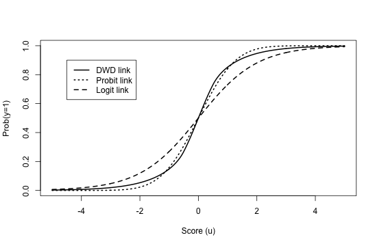
The conditional distribution for thus depends on its unconditional class probability , and its corresponding score :
| (5) |
Choice of does not influence posterior inference for in (4), but it is nevertheless important for the calibration of the predictive model and is discussed further in Section 6.1. Given , (5) defines a link function from to a probability in ; this function is smooth and comparable to a probit or logit link. Figure 1 plots this function under equal class proportions, .
4.2 Prior distribution of
Estimating and via maximizing the likelihood under model (5) would perform poorly in the HDLSS context, analogous to the poor performance of unconstrained probit or logistic regression models. However, the posterior distribution (4) also implies a “prior” distribution for that is not conditional on :
| (6) |
where
| (7) |
and
| (8) |
This prior facilitates shrinkage in two important ways that improve performance in HDLSS settings. Term (8) gives the kernel of a multivariate normal distribution for , in which the ’s are independent with mean and variance . This derives from the penalty in (2). There is a vast literature on the connection between -regularized regression (e.g., ridge regression) and using Gaussian priors on the coefficients in a Bayesian framework, as mentioned in Section 1. This shrinks the inferred coefficients toward , which improves performance in the HDLSS setting or in the presence of multicollinearity. Term (7) favors that correspond to directions in with high variability or bimodality. To illustrate, Figure 2 plots a single term of the product as a function of the DWD score when ,
| (9) |
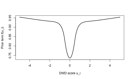
This term gives higher prior density to directions in for which the corresponding scores are not concentrated near , and are therefore more useful for discriminating a negative class from a positive class.
Theorem 2
The prior (6) does not define a proper density for . Improper priors are commonly used for a variety of Bayesian applications, and still provide a valid framework for inference if the posterior is proper (Taraldsen and Lindqvist, 2010; Sun et al., 2001). Nevertheless, it would be straightforward to modify the model to allow for shrinkage of , if one desired it to have a proper probability density without conditioning on .
4.3 Distribution of
No explicit probabilistic assumptions on are needed for the validity of the posterior and prior distributions in the previous two sections. However, it is informative to consider the broader implications of the model with respect to the distribution for . Without loss of generality we set and assume . Note that
where
Given any marginal density for (which may depend on ), ,
Thus, a marginal prior for exists but it depends on the distribution . Moreover,
implies that
Thus, given any marginal distribution for the data , it is possible to obtain the conditional distribution of given its class membership and the DWD vector .
5 Asymptotic normality of
It follows from the Bernstein-von Mises theorem (i.e., the “Bayesian central limit theorem”) (Ghosal, 1997) that the posterior distribution for approximates a multivariate normal distribution as . The limiting distribution can be derived precisely via a second-order Taylor expansion of the log of (4), about the mode . The resulting mean and covariance matrix are provided in Theorem 3.
Theorem 3
Note that this asymptotic approximation always exists and is directly computable given the DWD solution .
6 Extensions
6.1 Marginal class probabilities
The prior class probabilities and in (5) do not affect the posterior for in (4). Thus, they need not be specified for tasks that do not require a predictive model for , such as exploratory visualization or batch adjustment (Huang et al., 2012). However, their specification is important to obtain appropriately calibrated probabilities for classification. In particular, they must be considered carefully when the proportions in the training data differ from that of the target population. The ability to adjust the marginal class probabilities for out-of-sample prediction is useful, as the decision boundary for DWD () is sensitive to the class proportions used for training (Qiao et al., 2010; Qiao and Zhang, 2015). We let each observation have the same class membership probability a priori:
and by default we set . In other situations may be known and fixed at another value, or estimated as the sample proportion from class . Alternatively, one can give its own prior (e.g., ) and infer it with the rest of the Bayesian model; such an approach may be useful in (e.g.,) situation for which the ’s are only partially observed and the population class proportions are of interest.
6.2 Inference for
Rather than fixing the penalty parameter a priori, we recommend inferring its value within the Bayesian framework. For a given prior density , the conditional density for is
| (10) | ||||
where
| (11) |
In practice we use a prior for that is uniform over a large range, by default, . The impact of depends on the scale of and the number of observations , so the prior may need to be suitably modified for other scenarios.
6.3 Semi-supervised learning
The conditional distribution of on in (6) is not flat, and therefore observations for which are not observed can still inform . Consider the context in which observations are fully observed , have missing outcome , and . The full posterior distribution for is
This full posterior can be used for semi-supervised learning.
7 Posterior approximation
7.1 MCMC algorithm, fixed
To simulate from the posterior distribution for (4), we implement a “Metropolis-in-Gibbs” algorithm (Carlin and Louis, 2008). That is, we iteratively draw each from its conditional distribution given the current values of the rest of the parameters , ; each conditional draw is accomplished via a Metropolis sub-step. For the Metropolis step, we generate proposals from a normal distribution with mean given by the previous value for and a variance that is adaptively scaled over the course of the algorithm. We initialize the Markov chain at the posterior mode, which can be identified using existing software for DWD; we use the sdwd package for this initialization.
7.2 Inference for
Inference for can be accomplished by iteratively simulating from its full conditional distribution (10) to update its value within the Gibbs sampling algorithm in Section 7.1. However, this is not straightforward, because the integral (11) does not have a closed form. In our implementation, we first estimate over a grid of values that span the range of the prior for . For this, we utilize the fact that resembles a Gaussian kernel to approximate the integral via Monte Carlo with simulated random normal vectors. Given for ,
Using this approximation, we estimate for each , and then linearly interpolate on the log-scale to approximate the full function over the range of the prior for . Posterior estimation then proceeds as in Section 7.1, with an additional Metropolis sub-step to update the value of . The full algorithm for posterior sampling is given in Appendix B.
7.3 Computational considerations
In practice, we find that MCMC cycles yield appropriate coverage of the posterior when is fixed (see Section 8.1) and are sufficient when is inferred. On a single CPU, MCMC iterations takes approximately minutes for a dataset of size (comparable to the data considered in Section 9) and computing time scales linearly with the dimension . Thus, full posterior inference via MCMC is feasible for most applications (with patience), but computing time can be a limitation.
8 Simulations
We consider three distinct simulation scenarios, and multiple conditions under each scenario, to illustrate and validate several aspects of Bayesian DWD.
In Section 8.1 we simulate from a data generating scheme that matches the assumed prior and likelihood exactly. Under this scenario, we confirm that posterior inferences using the MCMC algorithms in Section 7 are appropriately calibrated regardless of the marginal distribution for . We compare to results using the normal approximation in Section 5 and a bootstrapping approach.
In Section 8.2 we consider a scenario in which the two classes are defined by different multivariate normal distributions. Under this scenario we demonstrate the robustness of Bayesian DWD to its model assumptions, assess the sensitivity of results to the tuning parameter , and validate model-based inference for .
In Section 8.3 we consider different scenarios for which not all of the outcomes are observed to illustrate potential benefits and limitations of the semi-supervised approach.
8.1 Assumed model simulation
Here we fix and simulate data from the assumed model as follows:
-
1.
Generate according to a specified probability distribution,
-
2.
Generate from its conditional prior (via a Metropolis-Hastings algorithm), given
-
3.
For , compute the score and generate according to its class probabilities defined by (5).
As manipulated conditions, we consider three values for ( or ), two configurations of and ( or ), and three different probability distributions for : (1) entries are simulated independently from a Uniform distribution, (2) entries are simulated independently from an Exponential distribution centered to have mean , and (3) each column is simulated from the following mixture of multivariate normal distributions:
| (12) |
where the entries of and are generated independently from a N distribution.
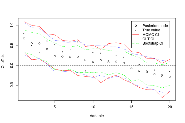
For each set of manipulated conditions, we generate datasets under the assumed model and approximate the posterior distribution for using the MCMC algorithm in Section 7.1. We construct 95% Bayesian credible intervals for and the scores based on the posterior samples. We also consider credible intervals constructed using the posterior mode and the asymptotic approximation in Theorem 3 (i.e., the CLT approximation), and confidence intervals based on the percentiles of non-parametric bootstrap resamples as in Lyu et al. (2017).
Table 1 gives the average coverage rates for the true values under each set of conditions and the three different approaches to inference. The credible intervals using MCMC all have nominal coverage rates, which validates the algorithm. The CLT approximation gives appropriate coverage in several instances, even when . However, it performs less well when is smaller and has relatively lower coverage rates for the scores . The bootstrap percentile approach yields more narrow intervals and tends to undercover in all cases. As a representative example, Figure 3 plots the mode and 95% intervals for the coefficients for an instance under the Uniform scenario with , and ; this shows close agreement between the MCMC and CLT intervals, and the bootstrap intervals are universally more narrow.
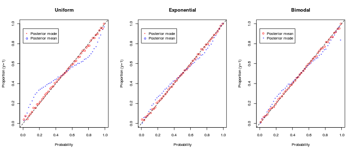
To assess the calibration of estimated class probabilities, we generate a new set of observations under the true model as a “test” set for each instance of the simulation. We compute the class probabilities for each test case, given the posterior fit to the or training cases. We group the estimated probabilities into narrow bins of length (, etc.) and consider the proportion of cases with in each bin. Figure 4 plots these proportions, aggregated across all conditions, vs. the midpoint of each bin. Using the posterior mean, the empirical proportions match the estimated probabilities perfectly, confirming that the model is well-calibrated and again validating the MCMC procedure. Using the posterior mode, the relationship deviates slightly but still tends to provide a reasonable fit in most cases.
| MCMC | CLT | BOOT | |||||||
|---|---|---|---|---|---|---|---|---|---|
| Distribution | |||||||||
| Uniform | 0.94 | 0.94 | 0.95 | 0.85 | 0.16 | 0.42 | |||
| Uniform | 0.94 | 0.94 | 0.95 | 0.85 | 0.23 | 0.50 | |||
| Uniform | 0.94 | 0.94 | 0.95 | 0.96 | 0.20 | 0.45 | |||
| Uniform | 0.94 | 0.94 | 0.92 | 0.85 | 0.46 | 0.55 | |||
| Uniform | 0.95 | 0.95 | 0.95 | 0.95 | 0.53 | 0.65 | |||
| Uniform | 0.94 | 0.94 | 0.95 | 0.95 | 0.24 | 0.32 | |||
| Exponential | 0.96 | 0.94 | 0.92 | 0.91 | 0.61 | 0.69 | |||
| Exponential | 0.95 | 0.95 | 0.96 | 0.95 | 0.62 | 0.71 | |||
| Exponential | 0.94 | 0.94 | 0.96 | 0.96 | 0.34 | 0.41 | |||
| Exponential | 0.94 | 0.95 | 0.92 | 0.85 | 0.39 | 0.49 | |||
| Exponential | 0.94 | 0.95 | 0.94 | 0.91 | 0.53 | 0.63 | |||
| Exponential | 0.94 | 0.94 | 0.95 | 0.96 | 0.40 | 0.52 | |||
| Bimodal | 0.95 | 0.96 | 0.94 | 0.91 | 0.61 | 0.66 | |||
| Bimodal | 0.94 | 0.95 | 0.96 | 0.95 | 0.66 | 0.73 | |||
| Bimodal | 0.93 | 0.94 | 0.96 | 0.96 | 0.39 | 0.46 | |||
| Bimodal | 0.94 | 0.94 | 0.92 | 0.85 | 0.37 | 0.47 | |||
| Bimodal | 0.95 | 0.95 | 0.94 | 0.90 | 0.51 | 0.60 | |||
| Bimodal | 0.94 | 0.95 | 0.96 | 0.96 | 0.40 | 0.61 | |||
8.2 Two-class multivariate normal simulation
Here we generate data according to a two-class multivariate normal distribution, in which each class has a different mean vector, as follows:
-
1.
Generate -dimensional mean vectors and , with independent entries from a N distribution.
-
2.
Set for and for .
-
3.
For , generate via
Note that this scenario differs from the ‘Bimodal’ case in Section 8.1 (12); for that scenario, membership in a given mixture component (defined by and ) does not necessarily correspond to the supervised class labels . The present scenario does not precisely match our assumed model. The “true” (i.e., oracle) probabilistic link between and in this scenario corresponds to a probit link with coefficients that are proportional to the mean difference vector ; as shown in Figure 1 the link for Bayesian DWD is not a probit, but it is close.
We fix and consider different levels of signal () and different dimensions () as manipulated conditions. For each instance, we approximate the posterior separately with fixed at each of possible values, that range from to and are equally spaced on a log scale. For each case we compute the Kullback-Leibler divergence (KL-divergence) of the estimated class probabilities from the oracle model. For each case we also generate a test set of samples and evaluate (1) the misclassification rate on the test samples using a posterior predictive probability of as a threshold, and the mean squared error (MSE) of the predicted class probabilities for class 1 () from the true class memberships as
Figure 5 plots these metrics as a function of for the different conditions. In general, lower values of perform better when the distinguishing signal is stronger. This is intuitive, as can be considered an inverse scale parameter for , and larger magnitudes for correspond to probabilities closer to and . The misclassification rate is robust to the value of , but its specification is important to achieve well-calibrated probabilities.
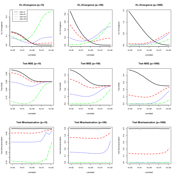
Motivated by the sensitivity of the estimated probabilities to , we also approximate the posterior with a uniform prior on as in Section 6.2. Table 2 summarizes the posterior mean for under each set of conditions, and compares the performance of the model with uniform prior on with that of the best performing fixed value of for each metric. The model with a uniform prior performs comparatively well across the different scenarios, and the posterior mean for appropriately ranges from very high values when the signal is nonexistent to low values when the signal is strong. However, for the conditions with and strong signal the posterior mean is substantially larger than the best performing values of ; this is likely because the model fits well and perfectly classifies the data with probabilities close to or for a wide range of values (see Figure 5), so there is not strong evidence to distinguish between different values of in this range.
| s2n ( | KL() | KL() | MSE() | MSE() | ||||
|---|---|---|---|---|---|---|---|---|
| 70.21 | 128.00 | 128.00 | 0.00 | 0.00 | 0.25 | 0.25 | ||
| 70.82 | 2.00 | 2.00 | 0.02 | 0.02 | 0.25 | 0.25 | ||
| 31.27 | 0.50 | 1.00 | 0.06 | 0.02 | 0.24 | 0.22 | ||
| 0.10 | 0.12 | 0.12 | 0.06 | 0.05 | 0.11 | 0.11 | ||
| 100 | 74.56 | 128.00 | 64.00 | 0.00 | 0.00 | 0.25 | 0.25 | |
| 100 | 22.55 | 1.00 | 2.00 | 0.15 | 0.10 | 0.24 | 0.22 | |
| 100 | 0.14 | 0.12 | 0.50 | 0.11 | 0.10 | 0.11 | 0.10 | |
| 100 | 0.11 | 0.01 | 0.02 | 0.03 | 0.01 | 0.00 | 0.00 | |
| 1000 | 44.79 | 128.00 | 128.00 | 0.02 | 0.00 | 0.25 | 0.25 | |
| 1000 | 3.11 | 0.03 | 0.50 | 0.21 | 0.06 | 0.11 | 0.09 | |
| 1000 | 0.63 | 0.01 | 0.03 | 0.07 | 0.01 | 0.00 | 0.00 | |
| 1000 | 1.82 | 0.01 | 0.01 | 0.04 | 0.00 | 0.00 | 0.00 |
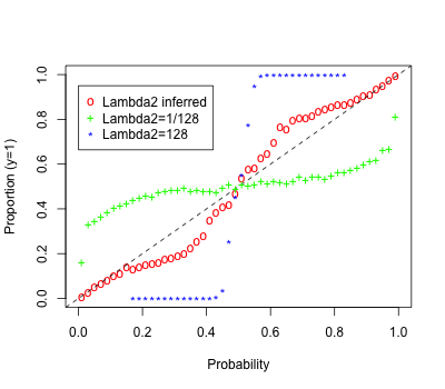
In Figure 6 we consider the overall calibration of the fitted probabilities across the different conditions, as in Section 8.1. This shows clearly that fixing at a large value () can yield overly conservative estimated probabilities and a relatively small value () can yield overly confident probabilities. The model in which is inferred with a uniform prior is mostly well-calibrated but does show some deviations from the estimated probabilities and empirical proportions. These deviations are likely in part due to the fact that the assumed probabilistic link does not perfectly match the true generative model.
8.3 Semi-supervised simulation
Here we generate data in which some of the class labels may be unknown, to illustrate a semi-supervised approach. We consider two scenarios. For the first scenario, the observations are generated exactly as in Section 8.2 with and . For the second scenario, and entries of each are generated independently from a distribution; then class labels are defined deterministically by the sign of , where the entries of are generated from a standard normal distribution. The key difference between these two scenarios, for our purpose, is that the first scenario (bimodal) has an underlying cluster structure that distinguishes the two classes whereas the second (unimodal) does not. So, we expect to improve performance by considering unlabeled data for the bimodal scenario but not the unimodal scenario.
As manipulated conditions, we vary the number of observations with observed ( and with unobserved () in our training set, for each of the bimodal and unimodal scenarios. For each combination of conditions, we generate datasets, use MCMC to approximate the posterior, and consider the resulting misclassification rates for a test set. The average test misclassification rates under each set of conditions are shown in Table 3. This shows that for the bimodal scenario a semi-supervised analysis with a large number of unlabeled observations can improve performance dramatically; the misclassification rates for observed and unobserved are comparable to that with observed. As expected, including data without observed class labels does not help in the unimodal scenario; however, it does not lead to a substantial decrease in performance.
| unobserved () | ||||||
|---|---|---|---|---|---|---|
| Scenario | observed () | |||||
| Bimodal | 0.164 | 0.138 | 0.145 | 0.081 | 0.019 | |
| Bimodal | 0.077 | 0.077 | 0.080 | 0.053 | 0.014 | |
| Bimodal | 0.038 | 0.035 | 0.032 | 0.036 | 0.020 | |
| Bimodal | 0.019 | 0.021 | 0.019 | 0.020 | 0.017 | |
| Unimodal | 0.444 | 0.451 | 0.425 | 0.410 | 0.432 | |
| Unimodal | 0.392 | 0.390 | 0.402 | 0.395 | 0.412 | |
| Unimodal | 0.280 | 0.266 | 0.272 | 0.280 | 0.297 | |
| Unimodal | 0.098 | 0.102 | 0.091 | 0.104 | 0.113 | |
9 Application to breast cancer genomics
As a real data application, we consider classifying breast cancer (BRCA) tumor subtypes using data on microRNA (miRNA) abundance that are publicly available from the Cancer Genome Atlas (TCGA). We use miRNA-Seq data for BRCA tumor samples from different individuals, that was previously curated for a pan-cancer clustering application (Hoadley et al., 2018). The tumors are classified into one of canonical subtypes based on the PAM classifier for gene (mRNA) expression (Parker et al., 2009): Luminal A (LumA) (), Luminal B (LumB) (), Her2 ), and Basal (). Previous exploratory analysis have shown that miRNA data shares some of the same BRCA subtype distinctions as gene expression (Park and Lock, 2020; Lock and Dunson, 2013). Here, we examine the power of miRNAs to distinguish the subtypes using a supervised approach.
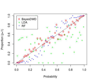
The miRNA expression read counts were log()-transformed and centered to have mean . After transformation, we keep miRNAs with standard deviation greater than , leaving miRNAs. We consider separate classification tasks to discriminate each pair of subtypes, giving comparisons. For each comparison, we apply (1) Bayesian DWD (BayesDWD) with uniform prior on , (2) DWD (i.e., the posterior mode) via the R package sdwd, (3) SVM via the package e1071, (4) random forest classification (Breiman, 2001) via the package randomForest, and (5) LDA via the package MASS. We assess each method by the average misclassification rate on the test sets under 10-fold cross-validation. The results are shown in Table 4. Bayesian DWD, DWD, and SVM have similar classification performance across the different comparisons, while random forests and LDA perform less well by comparison. For methods that give a class probability we consider the calibration of the estimated probabilities on the test sets vs. their empirical class proportions, as in Section 8.1. Figure 7 shows that the probabilities inferred for Bayesian DWD are overall well-calibrated. The probabilities under the random forest are also reasonable, but tend toward being over-conservative. The probabilities for LDA are not well-calibrated. LDA suffers from over-fitting in situations with higher dimension and lower sample size; for this application, the vast majority (93%) of predicted probabilities using LDA are below or above , leaving limited data for the remaining bins.
| Comparison | BayesDWD | DWD | SVM | RF | LDA |
|---|---|---|---|---|---|
| LumA vs. LumB | 0.168 | 0.156 | 0.158 | 0.186 | 0.296 |
| LumA vs. Her2 | 0.054 | 0.045 | 0.059 | 0.070 | 0.178 |
| LumA vs. Basal | 0.026 | 0.028 | 0.025 | 0.030 | 0.084 |
| LumB vs. Her2 | 0.129 | 0.124 | 0.155 | 0.169 | 0.188 |
| LumB vs. Basal | 0.046 | 0.043 | 0.044 | 0.047 | 0.137 |
| Her2 vs. Basal | 0.066 | 0.064 | 0.053 | 0.075 | 0.111 |
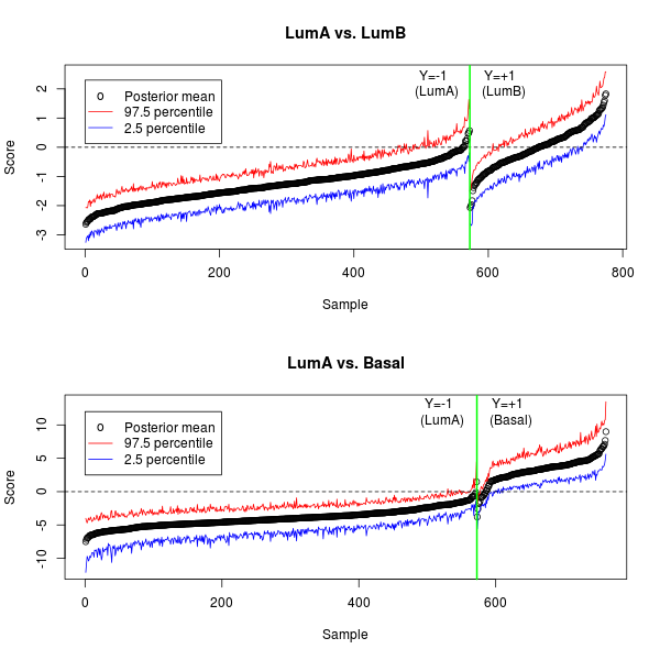
To illustrate the Bayesian DWD results, we focus on the comparison with the best classification accuracy from Table 4 (LumA vs. Basal) and the comparison with the worst classification accuracy (LumA vs. LumB). Figure 8 plots the posterior mean of the DWD scores and their credible intervals for each comparison. Note that the DWD scores are almost perfectly separated for LumA vs. Basal, but not for LumA vs. LumB. The credible intervals for each plot help to understand the level of uncertainty in the discriminating projections.
10 Discussion
The Bayesian formulation of DWD is straightforward to modify or extend via changes to the likelihood or prior. As a future direction, we are interested in extending the model to accommodate multiple sources of data (e.g., multiple ’omics or clinical sources) or data with multiway structure (Lyu et al., 2017). In this article we have focused on the original and most widely used version of DWD, but the Bayesian framework may be extended for other versions including multi-class DWD (Huang et al., 2013), weighted DWD (Qiao et al., 2010), sparse DWD (Wei et al., 2016), and kernel DWD (Wang and Zou, 2018, 2019). Additionally, a generalized version of DWD was introduced in (Hall et al., 2005), wherein the distances in (2) are raised to a power . The choice of modifies the loss function in (3) (Wang and Zou, 2018), which in turn affects the probabilistic link (5); the Bayesian formulation is potentially very useful in this context, because one can put a prior on and infer it within the model.
Computing time and resources can limit a fully Bayesian treatment of DWD for some applications, as discussed in Section 7.3. In such cases, the DWD solution can still be interpreted as a posterior mode to give point estimates for class probabilities, and the normal approximation in Section 5 can be used to quickly assess uncertainty in the estimated coefficients. Alternative computational approaches that facilitate a fully Bayesian treatment for massive datasets are worth pursuing.
Acknowledgments
This work was supported by the National Institutes of Health (NIH) grant R01-GM130622.
A Proofs
Theorem 1
If , , and where for some and for some , then in (4) gives a proper probability density function.
Proof Without loss of generality assume and . Define
By (4), . It suffices to show that (i) is non-negative and (ii) has finite integral over and . Condition (i) is trivially satisfied. For condition (ii), note that , where is defined in (3). Thus,
Let define the -norm, and note that . For fixed ,
It follows that
Theorem 2
Proof Define , where and are defined in (7) and (8). Note that and are always non-negative, and term is alway less than . Thus,
B Algorithm
Here we describe in detail the algorithm to simulate draws from their joint posterior distribution . First, estimate the normalizing function as described in Section 7.2. Then, initialize to a positive value (e.g., ) and initialize to the conditional posterior mode using the sdwd package (Wang and Zou, 2016) or other software. The algorithm is given below for iterations .
-
1.
For , update as follows:
-
(a)
Generate proposal
-
(b)
Set and
-
(c)
Compute , with the numerator and denominator given by (4)
-
(d)
Generate
-
(e)
If set , otherwise set .
-
(a)
-
2.
Update as follows:
-
(a)
Generate proposal
-
(b)
Compute , with the numerator and denominator given by (4)
-
(c)
Generate
-
(d)
If set , otherwise set .
-
(a)
-
3.
Update as follows:
-
(a)
Generate proposal by where
-
(b)
Compute
-
(c)
Generate
-
(d)
If set , otherwise set .
-
(a)
-
4.
Set to half of the sample variance of .
Note that if is fixed, step (c) above can be skipped. The adaptive updating of the proposal variance in step (d) is not necessary for the validity of the algorithm, but can improve mixing considerably when the approximate scale of the coefficients is uncertain.
References
- Breiman (2001) L. Breiman. Random forests. Machine learning, 45(1):5–32, 2001.
- Carlin and Louis (2008) B. P. Carlin and T. A. Louis. Bayesian methods for data analysis. CRC Press, 2008.
- Cortes and Vapnik (1995) C. Cortes and V. Vapnik. Support-vector networks. Machine learning, 20(3):273–297, 1995.
- Ghosal (1997) S. Ghosal. A review of consistency and convergence of posterior distribution. In Varanashi Symposium in Bayesian Inference, Banaras Hindu University, 1997.
- Hall et al. (2005) P. Hall, J. S. Marron, and A. Neeman. Geometric representation of high dimension, low sample size data. Journal of the Royal Statistical Society: Series B (Statistical Methodology), 67(3):427–444, 2005.
- Henao et al. (2014) R. Henao, X. Yuan, and L. Carin. Bayesian nonlinear support vector machines and discriminative factor modeling. In Advances in neural information processing systems, pages 1754–1762, 2014.
- Hoadley et al. (2018) K. A. Hoadley, C. Yau, T. Hinoue, D. M. Wolf, A. J. Lazar, E. Drill, R. Shen, A. M. Taylor, A. D. Cherniack, V. Thorsson, et al. Cell-of-origin patterns dominate the molecular classification of 10,000 tumors from 33 types of cancer. Cell, 173(2):291–304, 2018.
- Hsiang (1975) T. Hsiang. A Bayesian view on ridge regression. Journal of the Royal Statistical Society: Series D (The Statistician), 24(4):267–268, 1975.
- Huang et al. (2012) H. Huang, X. Lu, Y. Liu, P. Haaland, and J. Marron. R/DWD: distance-weighted discrimination for classification, visualization and batch adjustment. Bioinformatics, 28(8):1182–1183, 2012.
- Huang et al. (2013) H. Huang, Y. Liu, Y. Du, C. M. Perou, D. N. Hayes, M. J. Todd, and J. S. Marron. Multiclass distance-weighted discrimination. Journal of Computational and Graphical Statistics, 22(4):953–969, 2013.
- Liu et al. (2011) Y. Liu, H. H. Zhang, and Y. Wu. Hard or soft classification? large-margin unified machines. Journal of the American Statistical Association, 106(493):166–177, 2011.
- Lock and Dunson (2013) E. F. Lock and D. B. Dunson. Bayesian consensus clustering. Bioinformatics, 29(20):2610–2616, 2013.
- Lyu et al. (2017) T. Lyu, E. F. Lock, and L. E. Eberly. Discriminating sample groups with multi-way data. Biostatistics, 18(3):434–450, 2017.
- Marron et al. (2007) J. Marron, M. J. Todd, and J. Ahn. Distance-weighted discrimination. Journal of the American Statistical Association, 102(480):1267–1271, 2007.
- Park and Lock (2020) J. Y. Park and E. F. Lock. Integrative factorization of bidimensionally linked matrices. Biometrics, 76(1):61–74, 2020.
- Park and Casella (2008) T. Park and G. Casella. The Bayesian lasso. Journal of the American Statistical Association, 103(482):681–686, 2008.
- Parker et al. (2009) J. S. Parker, M. Mullins, M. C. Cheang, S. Leung, D. Voduc, T. Vickery, S. Davies, C. Fauron, X. He, Z. Hu, et al. Supervised risk predictor of breast cancer based on intrinsic subtypes. Journal of clinical oncology, 27(8):1160, 2009.
- Qiao and Zhang (2015) X. Qiao and L. Zhang. Flexible high-dimensional classification machines and their asymptotic properties. The Journal of Machine Learning Research, 16(1):1547–1572, 2015.
- Qiao et al. (2010) X. Qiao, H. H. Zhang, Y. Liu, M. J. Todd, and J. S. Marron. Weighted distance weighted discrimination and its asymptotic properties. Journal of the American Statistical Association, 105(489):401–414, 2010.
- Sollich (2002) P. Sollich. Bayesian methods for support vector machines: Evidence and predictive class probabilities. Machine learning, 46(1-3):21–52, 2002.
- Sun et al. (2001) D. Sun, R. K. Tsutakawa, and Z. He. Propriety of posteriors with improper priors in hierarchical linear mixed models. Statistica Sinica, pages 77–95, 2001.
- Taraldsen and Lindqvist (2010) G. Taraldsen and B. H. Lindqvist. Improper priors are not improper. The American Statistician, 64(2):154–158, 2010.
- Wang and Zou (2016) B. Wang and H. Zou. Sparse distance weighted discrimination. Journal of Computational and Graphical Statistics, 25(3):826–838, 2016.
- Wang and Zou (2018) B. Wang and H. Zou. Another look at distance-weighted discrimination. Journal of the Royal Statistical Society: Series B (Statistical Methodology), 80(1):177–198, 2018.
- Wang and Zou (2019) B. Wang and H. Zou. A multicategory kernel distance weighted discrimination method for multiclass classification. Technometrics, 61(3):396–408, 2019.
- Wei et al. (2016) S. Wei, C. Lee, L. Wichers, and J. Marron. Direction-projection-permutation for high-dimensional hypothesis tests. Journal of Computational and Graphical Statistics, 25(2):549–569, 2016.
- Witten and Tibshirani (2011) D. M. Witten and R. Tibshirani. Penalized classification using Fisher’s linear discriminant. Journal of the Royal Statistical Society: Series B (Statistical Methodology), 73(5):753–772, 2011.