This paper was converted on www.awesomepapers.org from LaTeX by an anonymous user.
Want to know more? Visit the Converter page.

Bayesian Dynamic Generalized Additive Model for Mortality during COVID-19 Pandemic

Wei Zhang111wei.zhang@usi.ch Università della Svizzera Italiana Antonietta Mira222antonietta.mira@usi.ch Università della Svizzera Italiana Ernst C. Wit333ernst.jan.camiel.wit@usi.ch Università della Svizzera Italiana
Abstract

While COVID-19 has resulted in a significant increase in global mortality rates, the impact of the pandemic on mortality from other causes remains uncertain. To gain insight into the broader effects of COVID-19 on various causes of death, we analyze an Italian dataset that includes monthly mortality counts for different causes from January 2015 to December 2020. Our approach involves a generalized additive model enhanced with correlated random effects. The generalized additive model component effectively captures non-linear relationships between various covariates and mortality rates, while the random effects are multivariate time series observations recorded in various locations, and they embody information on the dependence structure present among geographical locations and different causes of mortality. Adopting a Bayesian framework, we impose suitable priors on the model parameters. For efficient posterior computation, we employ variational inference, specifically for fixed effect coefficients and random effects, Gaussian variational approximation is assumed, which streamlines the analysis process. The optimisation is performed using a coordinate ascent variational inference algorithm and several computational strategies are implemented along the way to address the issues arising from the high dimensional nature of the data, providing accelerated and stabilised parameter estimation and statistical inference.

Keywords: generalized additive model, state space model, variational inference

1 Introduction

The COVID-19 pandemic has had profound impacts across the globe. Researches focus on various aspects such as health disparities linked to racial and socio-economic factors and the healthcare system’s adaptation in terms of testing, contact tracing, and vaccine rollouts (Kretzschmar et al.,, 2020; Peretti-Watel et al.,, 2020; Abedi et al.,, 2021). A key area of investigation is excess mortality, which provides an overarching view of the pandemic’s impact on human health. This includes factors such as government lockdown measures and disruptions to non-COVID healthcare services (Wang et al.,, 2022; Msemburi et al.,, 2023). While excess mortality offers a general perspective, examining the consequences of specific causes of death as a result of these factors during the pandemic is crucial for developing more targeted future mitigation strategies. For example, the pandemic has contributed to increases in deaths from chronic conditions as observed by Shiels et al., (2022). There also has been a rise in accidental deaths, homicides or suicides (Pell et al.,, 2020; Mitchell and Li,, 2021; Dmetrichuk et al.,, 2022). Contributing to this research field, we analyze Italian monthly death counts recorded in 21 Italian regions from 2015 to 2020, categorized according to the International Classification of Diseases, 10th Revision (ICD-10) (WHO,, 1992), to understand the effects on specific human mortality during the pandemic better.

We apply the generalized additive model (GAM) (Hastie and Tibshirani,, 1987; Hastie,, 2017) to study non-linear relationships between response, cause-specific mortality rate, and continuous covariates, including lockdown intensity level and age, in terms of smooth functions. GAMs have demonstrated considerable potential to study COVID-19 mortality (Koum Besson et al.,, 2021; Zhu et al.,, 2021; Basellini and Camarda,, 2022). In the more general context of spatial-temporal data modeling, GAMs are well-suited for analyzing changes over time and across different geographic regions, crucial in understanding the differentiating consequences. One way of employing GAMs to model the change of spatial pattern over time is via a tensor product smoother (Wood,, 2017; Feng,, 2022). Alternatively, Clark and Wells, (2023) introduce dynamic GAMs where extra dynamic spatial random effects are incorporated into the mean of response variable, offering a solution to forecasting discrete time series while estimating relevant nonlinear predictor associations that conventional generalized linear models (GLM) plus spatial temporal random effects are not able to account for (Nazia et al.,, 2022; Yin et al.,, 2023). In our study, we follow Clark and Wells, (2023)’s approach and assume that the mortality rate of specific cause in a region for a certain month combines a GAM regression component and random effects. The random effects are further assumed to be correlated as opposed to being independent, facilitating statistical inference on dependence structure between geographical regions and various causes of death (Rao and Molina,, 2015; Smith et al.,, 2015). We adopt a Bayesian approach and assign suitable priors on model parameters to better infer correlation structure from the data.

The model framework is a special case of non-Gaussian state space models where the observation equation is Poisson distribution. Inference with state space models includes filtering to estimate the current state given past observations and smoothing to estimate past states given all observations up to the current time (Petris et al.,, 2009; Durbin and Koopman,, 2012). Filtering and smoothing is exact in linear Gaussian state space models where Kalman Filter can be applied. When the model is non-Gaussian, particle filter approximates the states using a set of weighted particles (Doucet et al.,, 2001). The posterior samples in Clark and Wells, (2023) are drawn either in the Gibbs sampling software JAGS (Plummer et al.,, 2003) or with the Hamiltonian Monte Carlo in Stan (Carpenter et al.,, 2017). However, the approximation for the target deteriorates as the dimension increases (Beskos et al.,, 2014; Van Leeuwen et al.,, 2019). Due to the high dimensionality inherent in the data and model, these sampling algorithms are impractical. To address the issue, we use a variational inference algorithm for fast approximation (Jordan et al.,, 1999; Blei et al.,, 2017); more specifically, the joint variational density of fixed effect coefficients and random effects takes the Gaussian form. Various methods exist for optimizing the mean and variance of this approximating Gaussian distribution. For instance, Titsias and Lázaro-Gredilla, (2014) propose to parameterize the density in terms of its mean and a lower triangular scale matrix whereas Tan and Nott, (2018) incorporate sparsity in the Cholesky factors of the precision matrix. Both developed stochastic gradient methods for optimization. Our approach instead involves Newton’s method and fixed point iteration as in Arridge et al., (2018) to achieve faster convergence in fewer iterations. This aligns with recent advancements with recent development in Gaussian variational approximations for high-dimensional state space models (Quiroz et al.,, 2023), but distincts in that we do not define structure of the proposed variational approximation thanks to our chosen optimization technique.

The rest of the paper is organized as follows. In Section 2, we formulate the model and specify the priors imposed on parameters. In Section 3, we demonstrate how to derive the ELBO in this model setup and present the variational algorithm for posterior inferences. We then apply the model and the algorithm to the Italian monthly mortality data in Section 4. Finally, Section 5 gives some concluding remarks and points to future work.

2 Bayesian dynamic GAM

Let Yn,tY_{n,t} be the mortality count of instance nn at time tt, n=1,,N,t=1,,Tn=1,\dots,N,t=1,\dots,T. For each nn, covariates such as ordinal ana_{n} for age categorical gng_{n} for gender, lnl_{n} for LL geographical locations and knk_{n} for KK different causes of death are available. Additionally, we are interested in the lockdown effect on outcome variable Yn,tY_{n,t}, therefore we include a stringency index that quantifies the intensity of government restriction policies for each geographical location over time and we denote it by rn,tr_{n,t}, which depends on nn through lnl_{n}. We assume that Yn,tY_{n,t} is Poisson random variable with rate equal to

ϵn,texp[𝐱n𝜷𝜷+fr(rn,t)+fa(an)+fk,r(kn,rn,t)+fk,a(kn,an)+fg,a(gn,an)+zn,t]\epsilon_{n,t}\exp\left[\mathbf{x}^{\bm{\beta}}_{n}\bm{\beta}+f^{r}(r_{n,t})+f^{a}(a_{n})+f^{k,r}(k_{n},r_{n,t})+f^{k,a}(k_{n},a_{n})+f^{g,a}(g_{n},a_{n})+z^{*}_{n,t}\right]

where ϵn,t\epsilon_{n,t} is the offset, 𝐱n𝜷𝜷\mathbf{x}^{\bm{\beta}}_{n}\bm{\beta} are parametric terms which include gender effect. fr(rn,t)f^{r}(r_{n,t}) and fa(an)f^{a}(a_{n}) are natural cubic splines for government intervention effect and age effect respectively and they take the form

fr(r)=j=1Jujr(r)βjr,fa(a)=j=1Juja(a)βja,f^{r}\left(r\right)=\sum_{j=1}^{J}u^{r}_{j}\left(r\right)\beta^{r}_{j},\quad f^{a}\left(a\right)=\sum_{j=1}^{J}u^{a}_{j}\left(a\right)\beta^{a}_{j},

where JJ is the number of knots, ujr,ujau^{r}_{j},u^{a}_{j} are natural cubic spline bases, βjr\beta^{r}_{j} and βja\beta^{a}_{j} are coefficients to be estimated. The smoothness penalization terms associated with the bases are defined as

λ1r(𝜷r)S1r𝜷r+λ2r(𝜷r)S2r𝜷r,λ1a(𝜷a)S1a𝜷a+λ2a(𝜷a)S2a𝜷a.\lambda^{r}_{1}(\bm{\beta}^{r})^{\prime}S^{r}_{1}\bm{\beta}^{r}+\lambda^{r}_{2}(\bm{\beta}^{r})^{\prime}S^{r}_{2}\bm{\beta}^{r},\quad\lambda^{a}_{1}(\bm{\beta}^{a})^{\prime}S^{a}_{1}\bm{\beta}^{a}+\lambda^{a}_{2}(\bm{\beta}^{a})^{\prime}S^{a}_{2}\bm{\beta}^{a}.

Here S1r,S1r,S1a,S2aS^{r}_{1},S^{r}_{1},S^{a}_{1},S^{a}_{2} contain known coefficients. 𝜷r=(β1r,,βJr)\bm{\beta}^{r}=\left(\beta^{r}_{1},\dots,\beta^{r}_{J}\right)^{\prime} and 𝜷a=(β1a,,βJa)\bm{\beta}^{a}=\left(\beta^{a}_{1},\dots,\beta^{a}_{J}\right)^{\prime} are vectors of spline coefficients. From a Bayesian perspective, this is equivalent to imposing the following multivariate normal priors on 𝜷r\bm{\beta}_{r} and 𝜷a\bm{\beta}_{a}

𝜷r𝒩(𝟎,(λ1rS1r+λ2rS2r)1)\displaystyle\bm{\beta}^{r}\sim\mathcal{N}\left(\mathbf{0},\left(\lambda^{r}_{1}S^{r}_{1}+\lambda^{r}_{2}S^{r}_{2}\right)^{-1}\right)
𝜷a𝒩(𝟎,(λ1aS1a+λ2aS2a)1).\displaystyle\bm{\beta}^{a}\sim\mathcal{N}\left(\mathbf{0},\left(\lambda^{a}_{1}S^{a}_{1}+\lambda^{a}_{2}S^{a}_{2}\right)^{-1}\right).

λ1r,λ2r,λ1a\lambda^{r}_{1},\lambda^{r}_{2},\lambda^{a}_{1} and λ2a\lambda^{a}_{2} control the level of roughness.

As for the two-way interaction terms, fk,r(k,r)f^{k,r}(k,r) models interactions between cause of death and stringency index in a non-parametric manner. fk,a(k,a)f^{k,a}(k,a) accounts for interactions between causes of death and age while fg,a(g,a)f^{g,a}(g,a) captures interactions between gender and age. The three interactions terms are constructed in the following way. For each level kk of causes of death or each gg of gender, a unique spline is specified (Wood,, 2017). We formulate fk,r(k,r)f^{k,r}(k,r) as an example, fk,a(k,a)f^{k,a}(k,a) and fg,a(g,a)f^{g,a}(g,a) are modeled in a similar way. For each kk other than the baseline, fk,r(k,r)f^{k,r}(k,r) is assumed to be natural cubic spline such that

fk,r(k,r)=j=1Juk,jk,r(r)βk,jk,r.f^{k,r}(k,r)=\sum_{j=1}^{J}u^{k,r}_{k,j}\left(r\right)\beta^{k,r}_{k,j}.

The J(K1)J(K-1) dimensional vector 𝜷k,r=(β2,1k,r,,β2,Jk,r,β3,1k,r,βK,Jk,r)\bm{\beta}^{k,r}=\left(\beta^{k,r}_{2,1},\dots,\beta^{k,r}_{2,J},\beta^{k,r}_{3,1}\dots,\beta^{k,r}_{K,J}\right)^{\prime} is jointly penalised by S1k,rS^{k,r}_{1} and S2k,rS^{k,r}_{2} with smoothing parameters λ1k,r\lambda^{k,r}_{1} and λ2k,r\lambda^{k,r}_{2} and the penalisation term is λ1k,r(𝜷k,r)S1r𝜷k,r+λ2k,r(𝜷k,r)S2r𝜷k,r,\lambda^{k,r}_{1}(\bm{\beta}^{k,r})^{\prime}S^{r}_{1}\bm{\beta}^{k,r}+\lambda^{k,r}_{2}(\bm{\beta}^{k,r})^{\prime}S^{r}_{2}\bm{\beta}^{k,r}, which, in terms of Bayesian prior, translates to

𝜷k,r𝒩(𝟎,(λ1k,rS1k,r+λ2k,rS2k,r)1).\bm{\beta}^{k,r}\sim\mathcal{N}\left(\mathbf{0},\left(\lambda^{k,r}_{1}S^{k,r}_{1}+\lambda^{k,r}_{2}S^{k,r}_{2}\right)^{-1}\right).

The last term zn,tz^{*}_{n,t} embeds the spatial-temporal structure in the data; in fact, zn,tz^{*}_{n,t} depends on nn through lnl_{n} and knk_{n}, therefore in total, we have LKLK time series of length TT. zn,tz^{*}_{n,t} can be modeled with great flexibility. We make the following latent state assumption. Let 𝐳t=(z1,t,,zN,t)\mathbf{z}^{*}_{t}=(z^{*}_{1,t},\dots,z^{*}_{N,t})^{\prime} and 𝐳t=(z1,t,,zLK,t)\mathbf{z}_{t}=(z_{1,t},\dots,z_{LK,t})^{\prime} such that

𝐳t=(ILK𝟏)𝐳t,\mathbf{z}^{*}_{t}=\left(I_{LK}\bigotimes\mathbf{1}\right)\mathbf{z}_{t},

where 𝟏\mathbf{1} stands for a vector whose elements are all equal to 1. The dimension of 𝟏\mathbf{1} is determined by the number of age groups and gender. The assumption implies that residual mortality rates zn,tz^{*}_{n,t} of the same causes of death in the same region are identical regardless of age and gender, which is reasonable since we have already taken into account age and gender effect in GAM component. We further assume that marginally the latent state 𝐳t𝒩(𝝁,Σ)\mathbf{z}_{t}\sim\mathcal{N}\left(\bm{\mu},\Sigma\right) and P(𝐳t𝝁)P\left(\mathbf{z}_{t}-\bm{\mu}\right) follows a simple autoregressive (AR) process such that

P(𝐳t𝝁)=ΦP(𝐳t1𝝁)+ϵt,ϵt𝒩(𝟎,ILKΦΦ),P\left(\mathbf{z}_{t}-\bm{\mu}\right)=\Phi P\left(\mathbf{z}_{t-1}-\bm{\mu}\right)+\bm{\epsilon}_{t},\quad\bm{\epsilon}_{t}\sim\mathcal{N}\left(\mathbf{0},I_{LK}-\Phi\Phi^{\prime}\right),

where PP is an upper triangular matrix such that PP=Ω=Σ1P^{\prime}P=\Omega=\Sigma^{-1}, i.e. P are the Cholesky factors of the precision matrix Ω\Omega. Φ\Phi contains multivariate autoregressive coefficients. For simplicity, we require Φ\Phi to be diagonal with diagonal entries ϕ=c(ϕ1,,ϕLK)\bm{\phi}=c(\phi_{1},\dots,\phi_{LK})^{\prime} such that 1<ϕ1,,ϕLK<1-1<\phi_{1},\dots,\phi_{LK}<1. The pre-multiplying of 𝐳t\mathbf{z}_{t} by PP is to ensure that marginally 𝐳t𝒩(𝟎,Σ),t=0,,T\mathbf{z}_{t}\sim\mathcal{N}\left(\mathbf{0},\Sigma\right),t=0,\dots,T where Σ\Sigma incorporates dependence structure of geographical locations as well as mortality causes. Reorganizing 𝐳t\mathbf{z}_{t} as matrices ZtZ_{t} of size L×KL\times K, we assume that

ZtMN(𝝁,Σk,Σl),Z_{t}\sim\text{MN}\left(\bm{\mu},\Sigma^{k},\Sigma^{l}\right),

which is a matrix normal distribution equivalent to

𝐳t𝒩(𝝁,ΣkΣl),\mathbf{z}_{t}\sim\mathcal{N}\left(\bm{\mu},\Sigma^{k}\bigotimes\Sigma^{l}\right),

where \bigotimes stands for the Kronecker product between Σk\Sigma^{k} and Σl\Sigma^{l}, the covariance matrices of the causes of death dependence and regional dependence respectively. We impose the following priors on the model parameters. Firstly, 𝝁\bm{\mu} is assigned a normal prior 𝒩(𝟎,σμ2ILK)\mathcal{N}\left(\mathbf{0},\sigma^{2}_{\mu}I_{LK}\right). Ωk=(Σk)1\Omega^{k}=\left(\Sigma^{k}\right)^{-1} is the precision matrix that underlines the conditional independence of mortality causes. For simplicity, we stick to the usual Wishart distribution

ΩkWishart(δk,θkIK).\Omega^{k}\sim\text{Wishart}\left(\delta^{k},\theta^{k}I_{K}\right).

The same reasoning applies to the precision matrix Ωl=(Σl)1\Omega^{l}=\left(\Sigma^{l}\right)^{-1} and it follows that

ΩlWishart(δl,θlIL).\Omega^{l}\sim\text{Wishart}\left(\delta^{l},\theta^{l}I_{L}\right).

We complete the model with a hierarchy of prior specification on the linear regression coefficients, on penalization parameters that control smoothness of splines and on the autoregressive coefficients, on the cause specific mean. Denoting by 𝐱n\mathbf{x}_{n} the vector containing 𝐱n𝜷\mathbf{x}^{\bm{\beta}}_{n} and all bases in GAMs for nn, the hierarchical model can be summarized as

Yn,tPoisson[ϵn,texp(𝐱n𝜷+zn,t)],𝜷=(𝜷,(𝜷r),(𝜷a),(𝜷k,r),(𝜷k,a),(𝜷g,a)),\displaystyle Y_{n,t}\sim\text{Poisson}\left[\epsilon_{n,t}\exp\left(\mathbf{x}_{n}\bm{\beta}^{*}+z^{*}_{n,t}\right)\right],\quad\bm{\beta}^{*}=\left(\bm{\beta}^{\prime},\left(\bm{\beta}^{r}\right)^{\prime},\left(\bm{\beta}^{a}\right)^{\prime},\left(\bm{\beta}^{k,r}\right)^{\prime},\left(\bm{\beta}^{k,a}\right)^{\prime},\left(\bm{\beta}^{g,a}\right)^{\prime}\right)^{\prime},
𝜷𝒩(𝟎,σβ2I),𝜷r𝒩(𝟎,(λ1rS1r+λ2rS2r)1),𝜷a𝒩(𝟎,(λ1aS1a+λ2aS2a)1),\displaystyle\bm{\beta}\sim\mathcal{N}\left(\mathbf{0},\sigma^{2}_{\beta}I\right),\quad\bm{\beta}^{r}\sim\mathcal{N}\left(\mathbf{0},\left(\lambda^{r}_{1}S^{r}_{1}+\lambda^{r}_{2}S^{r}_{2}\right)^{-1}\right),\quad\bm{\beta}^{a}\sim\mathcal{N}\left(\mathbf{0},\left(\lambda^{a}_{1}S^{a}_{1}+\lambda^{a}_{2}S^{a}_{2}\right)^{-1}\right),
𝜷k,r𝒩(𝟎,(λ1k,rS1k,r+λ2k,rS2k,r)1),𝜷k,a𝒩(𝟎,(λ1k,aS1k,a+λ2k,aS2k,a)1),\displaystyle\bm{\beta}^{k,r}\sim\mathcal{N}\left(\mathbf{0},\left(\lambda^{k,r}_{1}S^{k,r}_{1}+\lambda^{k,r}_{2}S^{k,r}_{2}\right)^{-1}\right),\quad\bm{\beta}^{k,a}\sim\mathcal{N}\left(\mathbf{0},\left(\lambda^{k,a}_{1}S^{k,a}_{1}+\lambda^{k,a}_{2}S^{k,a}_{2}\right)^{-1}\right),
𝜷g,a𝒩(𝟎,(λ1g,aS1g,a+λ2g,aS2g,a)1),\displaystyle\bm{\beta}^{g,a}\sim\mathcal{N}\left(\mathbf{0},\left(\lambda^{g,a}_{1}S^{g,a}_{1}+\lambda^{g,a}_{2}S^{g,a}_{2}\right)^{-1}\right),
λ1r,λ2r,λ1a,λ2a,λ1k,r,λ2k,r,λ1k,a,λ2k,a,λ1g,a,λ2g,aGamma(αλ,βλ),\displaystyle\lambda^{r}_{1},\lambda^{r}_{2},\lambda^{a}_{1},\lambda^{a}_{2},\lambda^{k,r}_{1},\lambda^{k,r}_{2},\lambda^{k,a}_{1},\lambda^{k,a}_{2},\lambda^{g,a}_{1},\lambda^{g,a}_{2}\sim\text{Gamma}\left(\alpha_{\lambda},\beta_{\lambda}\right),
𝐳t=(ILK𝟏)𝐳t,\displaystyle\mathbf{z}^{*}_{t}=\left(I_{LK}\bigotimes\mathbf{1}\right)\mathbf{z}_{t},
P(𝐳t𝝁)=ΦP(𝐳t1𝝁)+ϵt,ϵt𝒩(𝟎,ILKΦΦ),𝝁𝒩(𝟎,σμ2ILK),\displaystyle P\left(\mathbf{z}_{t}-\bm{\mu}\right)=\Phi P\left(\mathbf{z}_{t-1}-\bm{\mu}\right)+\bm{\epsilon}_{t},\quad\bm{\epsilon}_{t}\sim\mathcal{N}\left(\mathbf{0},I_{LK}-\Phi\Phi^{\prime}\right),\quad\bm{\mu}\sim\mathcal{N}\left(\mathbf{0},\sigma^{2}_{\mu}I_{LK}\right),
Φ=diag(ϕ1,,ϕLK),ϕ1+12,,ϕLK+12i.i,dBeta(αϕ,βϕ),\displaystyle\Phi=\text{diag}\left(\phi_{1},\dots,\phi_{LK}\right),\quad\frac{\phi_{1}+1}{2},\dots,\frac{\phi_{LK}+1}{2}\overset{i.i,d}{\sim}\text{Beta}(\alpha_{\phi},\beta_{\phi}),
PP=Ω=ΩkΩl,ΩkWishart(δk,θkIK),ΩlWishart(δl,θlIL).\displaystyle\quad P^{\prime}P=\Omega=\Omega^{k}\bigotimes\Omega^{l},\quad\Omega^{k}\sim\text{Wishart}\left(\delta^{k},\theta^{k}I_{K}\right),\quad\Omega^{l}\sim\text{Wishart}\left(\delta^{l},\theta^{l}I_{L}\right).

3 Posterior inference via variational approximation

To make posterior inference, one may devise suitable Markov Chain Monte Carlo (MCMC) algorithms to obtain posterior samples. However, the algorithm may fail to deliver desirable convergent output within reasonable time when it is difficult to explore the geometry of the target distribution due to the sheer dimension of the data. Therefore we resort to variational inference approach for fast approximation. The target posterior distribution is

p(\displaystyle p\left(\right. 𝜷,𝝀,𝐳0:T,ϕ,𝝁,Ωk,Ωl𝐲)\displaystyle\bm{\beta}^{*},\bm{\lambda},\mathbf{z}_{0:T},\left.\bm{\phi},\bm{\mu},\Omega^{k},\Omega^{l}\mid\mathbf{y}\right)
p(𝐲𝜷,𝐳0,T)p(𝜷𝝀)p(𝝀)p(𝐳0:Tϕ,𝝁,Ωk,Ωl)p(𝝁)p(ϕ)p(Ωk)p(Ωl),\displaystyle\propto p\left(\mathbf{y}\mid\bm{\beta}^{*},\mathbf{z}_{0,T}\right)p\left(\bm{\beta}^{*}\mid\bm{\lambda}\right)p\left(\bm{\lambda}\right)p\left(\mathbf{z}_{0:T}\mid\bm{\phi},\bm{\mu},\Omega^{k},\Omega^{l}\right)p\left(\bm{\mu}\right)p\left(\bm{\phi}\right)p\left(\Omega^{k}\right)p\left(\Omega^{l}\right),

and the goal is to find the optimal q(𝜷,𝝀,𝐳0:T,𝝁,ϕ,Ωk,Ωl)q^{*}\left(\bm{\beta}^{*},\bm{\lambda},\mathbf{z}_{0:T},\bm{\mu},\bm{\phi},\Omega^{k},\Omega^{l}\right) from a pre-specified family of distributions such that the Kullback–Leibler (KL) divergence, defined as

KL[q()||p(𝐲)]=Eq[logq()p(𝐲)],\text{KL}\left[q\left(\cdot\right)||p\left(\cdot\mid\mathbf{y}\right)\right]=\text{E}_{q}\left[\log\frac{q\left(\cdot\right)}{p\left(\cdot\mid\mathbf{y}\right)}\right],

with expectation taken with respect to q()q\left(\cdot\right), is minimized. This is equivalent to maximizing the evidence lower bound (ELBO) given by

ELBO[p(𝐲)]=Eq[logp(𝐲𝜷,𝐳0,T)p(𝜷𝝀)p(𝐳0:Tϕ,𝝁,Ωk,Ωl)p(𝝀)p(𝝁)p(ϕ)p(Ωk)p(Ωl)q(𝜷,𝐳0:T,𝝀,𝝁,ϕ,Ωk,Ωl)].\begin{aligned} &\text{ELBO}\left[p\left(\cdot\mid\mathbf{y}\right)\right]\\ =&\text{E}_{q}\left[\log\frac{p\left(\mathbf{y}\mid\bm{\beta}^{*},\mathbf{z}_{0,T}\right)p\left(\bm{\beta}^{*}\mid\bm{\lambda}\right)p\left(\mathbf{z}_{0:T}\mid\bm{\phi},\bm{\mu},\Omega^{k},\Omega^{l}\right)p\left(\bm{\lambda}\right)p\left(\bm{\mu}\right)p\left(\bm{\phi}\right)p\left(\Omega^{k}\right)p\left(\Omega^{l}\right)}{q\left(\bm{\beta}^{*},\mathbf{z}_{0:T},\bm{\lambda},\bm{\mu},\bm{\phi},\Omega^{k},\Omega^{l}\right)}\right].\end{aligned}

We further assume that the family of candidate approximation q()q(\cdot) can be factorized as

q(𝜷,𝐳0:T,𝝀,𝝁,ϕ,Ωk,Ωl)=q(𝜷,𝐳0:T)q(𝝀)q(𝝁)q(ϕ)q(Ωk)q(Ωl),q\left(\bm{\beta}^{*},\mathbf{z}_{0:T},\bm{\lambda},\bm{\mu},\bm{\phi},\Omega^{k},\Omega^{l}\right)=q\left(\bm{\beta}^{*},\mathbf{z}_{0:T}\right)q\left(\bm{\lambda}\right)q\left(\bm{\mu}\right)q\left(\bm{\phi}\right)q\left(\Omega^{k}\right)q\left(\Omega^{l}\right), (1)

where q(𝜷,𝐳0:T)q\left(\bm{\beta}^{*},\mathbf{z}_{0:T}\right) is multivariate normal distribution with mean 𝐦\mathbf{m} and covariance matrix MM. This is essentially the variational Gaussian approximation (VGA) that has been widely implemented in literature and its theoretical properties when applied to Poisson data are studied by Arridge et al., (2018). MM can be full or it can be sparse block diagonal matrix so that there is no correlation between 𝜷\bm{\beta}^{*} and 𝐳0:T\mathbf{z}_{0:T}, which means that q(𝜷,𝐳0:T)q\left(\bm{\beta}^{*},\mathbf{z}_{0:T}\right) can be further factorized as the product of two multivariate normal densities, q(𝜷)q\left(\bm{\beta}^{*}\right) and q(𝐳0:T)q\left(\mathbf{z}_{0:T}\right). The sparse version of MM greatly reduces algorithm complexity. However, in our application, since the dimension of 𝐳0:T\mathbf{z}_{0:T} is overwhelmingly larger than 𝜷\bm{\beta}^{*}, the block diagonal assumption does not produce much gain; therefore we stick to the full matrix characterisation of MM. Furthermore, we choose the following variational densities implied by mean field approximation: for each element in 𝝀\bm{\lambda}, it is a point mass at λ1q,r,λ2q,r,λ1q,a,λ2q,a,λ1q,k,r,λ2q,k,r,λ1q,k,a,λ2q,k,a,λ1q,g,a,λ2q,g,a\lambda^{q,r}_{1},\lambda^{q,r}_{2},\lambda^{q,a}_{1},\lambda^{q,a}_{2},\lambda^{q,k,r}_{1},\lambda^{q,k,r}_{2},\lambda^{q,k,a}_{1},\lambda^{q,k,a}_{2},\lambda^{q,g,a}_{1},\lambda^{q,g,a}_{2}. Together they are 𝝀q\bm{\lambda}^{q}. The Dirac measure choice as a variational density avoids evaluating expectation with respect to otherwise non-trivial variational densities. For q(𝝁)q\left(\bm{\mu}\right), we assume independent normal approximation densities q(𝝁)=𝒩(𝝁q,diag[(𝝈q)2])q\left(\bm{\mu}\right)=\mathcal{N}\left(\bm{\mu}^{q},\text{diag}\left[\left(\bm{\sigma}^{q}\right)^{2}\right]\right). For q(ϕ)q\left(\bm{\phi}\right), even though it is analytically possible to compute the expectation when assuming that (ϕ1+1)/2i.i,dBeta(α1q,ϕ,β1q,ϕ),,(ϕLK+1)/2i.i,dBeta(αLKq,ϕ,βLKq,ϕ)(\phi_{1}+1)/2\overset{i.i,d}{\sim}\text{Beta}(\alpha^{q,\phi}_{1},\beta^{q,\phi}_{1}),\dots,(\phi_{LK}+1)/2\overset{i.i,d}{\sim}\text{Beta}(\alpha^{q,\phi}_{LK},\beta^{q,\phi}_{LK}), the optimization scheme we adapt diverges as only the means of beta variational distributions is identifiable, therefore we use Dirac measures on q(ϕ)q\left(\bm{\phi}\right) so they are ϕq\bm{\phi}^{q}. Finally, we set q(Ωk)=Wishart(δq,k,Dq,k)q(\Omega^{k})=\text{Wishart}(\delta^{q,k},D^{q,k}) and q(Ωl)=Wishart(δq,l,Dq,l)q(\Omega^{l})=\text{Wishart}(\delta^{q,l},D^{q,l}).

3.1 ELBO calculation

With (1), the ELBO can be written as the sum of expectations

ELBO[p(𝐲)]\displaystyle\text{ELBO}\left[p\left(\cdot\mid\mathbf{y}\right)\right]
=\displaystyle= Eq[logp(𝐲𝜷,𝐳0,T)p(𝜷𝝀)p(𝐳0:Tϕ,𝝁,Ωk,Ωl)q(𝜷,𝐳0:T)]+Eq(𝝀)[logp(𝝀))q(𝝀))]\displaystyle\text{E}_{q}\left[\log\frac{p\left(\mathbf{y}\mid\bm{\beta}^{*},\mathbf{z}_{0,T}\right)p\left(\bm{\beta}^{*}\mid\bm{\lambda}\right)p\left(\mathbf{z}_{0:T}\mid\bm{\phi},\bm{\mu},\Omega^{k},\Omega^{l}\right)}{q\left(\bm{\beta}^{*},\mathbf{z}_{0:T}\right)}\right]+\text{E}_{q(\bm{\lambda)}}\left[\log\frac{p\left(\bm{\lambda)}\right)}{q\left(\bm{\lambda)}\right)}\right]
+Eq(𝝁)[logp(𝝁)q(𝝁)]+Eq(ϕ)[logp(ϕ)q(ϕ)]+Eq(Ωk)[logp(Ωk)q(Ωk)]+Eq(Ωl)[logp(Ωl)q(Ωl)].\displaystyle+\text{E}_{q(\bm{\mu})}\left[\log\frac{p\left(\bm{\mu}\right)}{q\left(\bm{\mu}\right)}\right]+\text{E}_{q(\bm{\phi})}\left[\log\frac{p\left(\bm{\phi}\right)}{q\left(\bm{\phi}\right)}\right]+\text{E}_{q(\Omega^{k})}\left[\log\frac{p\left(\Omega^{k}\right)}{q\left(\Omega^{k}\right)}\right]+\text{E}_{q(\Omega^{l})}\left[\log\frac{p\left(\Omega^{l}\right)}{q\left(\Omega^{l}\right)}\right].

The first term on the right hand side of the equation bears most importance as it connects likelihood with prior and it is also the most computationally heavy part to optimize due to the dimension of 𝐳0,T\mathbf{z}_{0,T}. Denote the mean and covariance matrix of joint multivariate normal prior on 𝜷\bm{\beta}^{*} and 𝐳0:T\mathbf{z}_{0:T} by 𝐦0\mathbf{m}_{0} and M0M_{0}. M0M_{0} is block diagonal, whose upper diagonal block corresponds to the covariance of 𝜷\bm{\beta}^{*} and lower diagonal block is the vector autoregressive matrix that derives from the assumed 𝐳t\mathbf{z}_{t} dynamics. The lower diagonal block is

(ITP1)(ILKΦΦ2ΦT1ΦILKΦΦT2Φ2ΦILKΦT3ΦT1ΦT2ΦT3ILK)(IT(P1)).\left(I_{T}\bigotimes P^{-1}\right)\begin{pmatrix}I_{LK}&\Phi&\Phi^{2}&\cdots&\Phi^{T-1}\\ \Phi&I_{LK}&\Phi&\cdots&\Phi^{T-2}\\ \Phi^{2}&\Phi&I_{LK}&\cdots&\Phi^{T-3}\\ \vdots&\vdots&\vdots&\ddots&\vdots\\ \Phi^{T-1}&\Phi^{T-2}&\Phi^{T-3}&\cdots&I_{LK}\\ \end{pmatrix}\left(I_{T}\bigotimes\left(P^{-1}\right)^{\prime}\right).

It is more convenient to use the precision matrix as the term repeatedly appears in the object function that we aim to optimize. The precision matrix can be expressed as (ITP)R(ITP)\left(I_{T}\bigotimes P^{\prime}\right)R\left(I_{T}\bigotimes P\right) with

R=((ILKΦ2)1(ILKΦ2)1Φ𝟎𝟎(ILKΦ2)1Φ(ILKΦ2)1(ILK+Φ2)(ILKΦ2)1Φ𝟎𝟎(ILKΦ2)1Φ(ILKΦ2)1(ILK+Φ2)𝟎𝟎𝟎𝟎(ILKΦ2)1).R=\begin{pmatrix}(I_{LK}-\Phi^{2})^{-1}&-(I_{LK}-\Phi^{2})^{-1}\Phi&\mathbf{0}&\cdots&\mathbf{0}\\ -(I_{LK}-\Phi^{2})^{-1}\Phi&(I_{LK}-\Phi^{2})^{-1}(I_{LK}+\Phi^{2})&-(I_{LK}-\Phi^{2})^{-1}\Phi&\cdots&\mathbf{0}\\ \mathbf{0}&-(I_{LK}-\Phi^{2})^{-1}\Phi&(I_{LK}-\Phi^{2})^{-1}(I_{LK}+\Phi^{2})&\cdots&\mathbf{0}\\ \vdots&\vdots&\vdots&\ddots&\vdots\\ \mathbf{0}&\mathbf{0}&\mathbf{0}&\cdots&(I_{LK}-\Phi^{2})^{-1}\\ \end{pmatrix}.

The first terms is hence

Eq[logp(𝐲𝜷,𝐳0,T)p(𝜷𝝀)p(𝐳0:T𝝁,ϕ,Ωk,Ωl)q(𝜷,𝐳0:T)]\displaystyle\text{E}_{q}\left[\log\frac{p\left(\mathbf{y}\mid\bm{\beta}^{*},\mathbf{z}_{0,T}\right)p\left(\bm{\beta}^{*}\mid\bm{\lambda}\right)p\left(\mathbf{z}_{0:T}\mid\bm{\mu},\bm{\phi},\Omega^{k},\Omega^{l}\right)}{q\left(\bm{\beta}^{*},\mathbf{z}_{0:T}\right)}\right]
=\displaystyle= 𝐲X𝐦i=1NTϵiexp(𝐱i𝐦+12𝐱iM𝐱i)12[𝐦Eq(𝐦0)]Eq(M01)[𝐦Eq(𝐦0)]\displaystyle\mathbf{y}^{\prime}X\mathbf{m}-\sum_{i=1}^{NT}\epsilon_{i}\exp\left(\mathbf{x}^{\prime}_{i}\mathbf{m}+\frac{1}{2}\mathbf{x}^{\prime}_{i}M\mathbf{x}_{i}\right)-\frac{1}{2}\left[\mathbf{m}-\text{E}_{q}(\mathbf{m}_{0})\right]^{\prime}\text{E}_{q}\left(M_{0}^{-1}\right)\left[\mathbf{m}-\text{E}_{q}(\mathbf{m}_{0})\right]
12tr[Eq(M01)M]+12log|M|12tr[Eq(M01))COVq(𝐦0)]+12Eq(log|M01|)\displaystyle-\frac{1}{2}\text{tr}\left[\text{E}_{q}(M_{0}^{-1})M\right]+\frac{1}{2}\log|M|-\frac{1}{2}\text{tr}\left[\text{E}_{q}(M_{0}^{-1}))\text{COV}_{q}(\mathbf{m}_{0})\right]+\frac{1}{2}\text{E}_{q}\left(\log|M_{0}^{-1}|\right)
+constant\displaystyle+constant

Here, XX is a two-block design matrix. The left block matrix consists of all regressors while the right block is the kronecker product ILKT𝟏I_{LKT}\bigotimes\mathbf{1}. The length of vector 𝟏\mathbf{1} relies on specific data configuration; in our case, it equals the product between number of age groups and gender. 𝐱i\mathbf{x}_{i} is the column vector of ii-th row of the design matrix XX. The expected value Eq(𝐦0)=(𝟎,(𝟏T𝝁q))\text{E}_{q}(\mathbf{m}_{0})=(\mathbf{0}^{\prime},(\mathbf{1}_{T}\bigotimes\bm{\mu}^{q})^{\prime})^{\prime} and Eq(M01)\text{E}_{q}\left(M_{0}^{-1}\right) is

Eq(M01)=(1σβ2I𝟎𝟎𝟎𝟎λ1q,rS1r+λ2q,rS2r𝟎𝟎𝟎𝟎𝟎𝟎𝟎λ1q,g,aS1g,a+λ2q,g,aS2g,a𝟎𝟎𝟎𝟎𝟎Eq[(ITP)Eq(R)(ITP)]),\text{E}_{q}\left(M_{0}^{-1}\right)=\begin{pmatrix}\frac{1}{\sigma_{\beta}^{2}}I&\mathbf{0}&\cdots&\mathbf{0}&\mathbf{0}\\ \mathbf{0}&\lambda_{1}^{q,r}S_{1}^{r}+\lambda_{2}^{q,r}S_{2}^{r}&\cdots&\mathbf{0}&\mathbf{0}\\ \vdots&\vdots&\ddots&\mathbf{0}&\mathbf{0}\\ \mathbf{0}&\mathbf{0}&\mathbf{0}&\lambda_{1}^{q,g,a}S_{1}^{g,a}+\lambda_{2}^{q,g,a}S_{2}^{g,a}&\mathbf{0}\\ \mathbf{0}&\mathbf{0}&\mathbf{0}&\mathbf{0}&\text{E}_{q}\left[\left(I_{T}\bigotimes P^{\prime}\right)\text{E}_{q}(R)\left(I_{T}\bigotimes P\right)\right]\end{pmatrix},

where

Eq(R)=(Eq1(R)Eq2(R)𝟎𝟎Eq2(R)Eq3(R)Eq2(R)𝟎𝟎Eq2(R)Eq3(R)𝟎𝟎𝟎𝟎Eq1(R)),\text{E}_{q}\left(R\right)=\begin{pmatrix}\text{E}^{1}_{q}\left(R\right)&\text{E}^{2}_{q}\left(R\right)&\mathbf{0}&\cdots&\mathbf{0}\\ \text{E}^{2}_{q}\left(R\right)&\text{E}^{3}_{q}\left(R\right)&\text{E}^{2}_{q}\left(R\right)&\cdots&\mathbf{0}\\ \mathbf{0}&\text{E}^{2}_{q}\left(R\right)&\text{E}^{3}_{q}\left(R\right)&\cdots&\mathbf{0}\\ \vdots&\vdots&\vdots&\ddots&\vdots\\ \mathbf{0}&\mathbf{0}&\mathbf{0}&\cdots&\text{E}^{1}_{q}\left(R\right)\end{pmatrix},

with diagonal matrices

Eq1(R)=diag(11(ϕq)2),Eq2(R)=diag(ϕq1(ϕq)2),Eq3(R)=diag(1+(ϕq)21(ϕq)2).\text{E}^{1}_{q}\left(R\right)=\text{diag}\left(\frac{1}{1-(\bm{\phi}^{q})^{2}}\right),\quad\text{E}^{2}_{q}\left(R\right)=\text{diag}\left(-\frac{\bm{\phi}^{q}}{1-(\bm{\phi}^{q})^{2}}\right),\quad\text{E}^{3}_{q}\left(R\right)=\text{diag}\left(\frac{1+(\bm{\phi}^{q})^{2}}{1-(\bm{\phi}^{q})^{2}}\right).

Here we vectorize the function by writing its arguments in terms of vectors ϕq\bm{\phi}^{q}. The expectation is therefore

Eq[(ITP)Eq(R)(ITP)]=(Eq[PEq1(R)P]Eq[PEq2(R)P]𝟎𝟎Eq[PEq2(R)P]Eq[PEq3(R)P]Eq[PEq2(R)P]𝟎𝟎Eq[PEq2(R)P]Eq[PEq3(R)P]𝟎𝟎𝟎𝟎Eq[PEq1(R)P]).\text{E}_{q}\left[\left(I_{T}\bigotimes P^{\prime}\right)\text{E}_{q}(R)\left(I_{T}\bigotimes P\right)\right]=\begin{pmatrix}\text{E}_{q}\left[P^{\prime}\text{E}^{1}_{q}\left(R\right)P\right]&\text{E}_{q}\left[P^{\prime}\text{E}^{2}_{q}\left(R\right)P\right]&\mathbf{0}&\cdots&\mathbf{0}\\ \text{E}_{q}\left[P^{\prime}\text{E}^{2}_{q}\left(R\right)P\right]&\text{E}_{q}\left[P^{\prime}\text{E}^{3}_{q}\left(R\right)P\right]&\text{E}_{q}\left[P^{\prime}\text{E}^{2}_{q}\left(R\right)P\right]&\cdots&\mathbf{0}\\ \mathbf{0}&\text{E}_{q}\left[P^{\prime}\text{E}^{2}_{q}\left(R\right)P\right]&\text{E}_{q}\left[P^{\prime}\text{E}^{3}_{q}\left(R\right)P\right]&\cdots&\mathbf{0}\\ \vdots&\vdots&\vdots&\ddots&\vdots\\ \mathbf{0}&\mathbf{0}&\mathbf{0}&\cdots&\text{E}_{q}\left[P^{\prime}\text{E}^{1}_{q}\left(R\right)P\right]\end{pmatrix}.

Recall that PP=Ω=ΩkΩlP^{\prime}P=\Omega=\Omega^{k}\bigotimes\Omega^{l}, when the variational densities of precision matrices Ωk\Omega^{k} and Ωl\Omega^{l} are Wishart(δq,k,Dq,k)\text{Wishart}(\delta^{q,k},D^{q,k}) and Wishart(δq,l,Dq,l)\text{Wishart}(\delta^{q,l},D^{q,l}), the derived Cholesky upper triangular matrix PP can be written as P=(AkVq,k)(AlVq,l)P=\left(A^{k}V^{q,k}\right)\bigotimes\left(A^{l}V^{q,l}\right) with (Vq,kAk)AkVq,k=Ωk,(Vq,lAl)AlVq,l=Ωl(V^{q,k}A^{k})^{\prime}A^{k}V^{q,k}=\Omega^{k},(V^{q,l}A^{l})^{\prime}A^{l}V^{q,l}=\Omega^{l}. Vq,k,Vq,lV^{q,k},V^{q,l} are Cholesky factors of Dq,kD^{q,k} and Dq,lD^{q,l} and

Ak=(c1kn1,2kn1,3kn1,Kk0c2kn2,3kn2,Kk00c3kn3,Kk000cKk),Al=(c1ln1,2ln1,3ln1,Kl0c2ln2,3ln2,Kl00c3ln3,Kl000cKl),A^{k}=\begin{pmatrix}c^{k}_{1}&n^{k}_{1,2}&n^{k}_{1,3}&\cdots&n^{k}_{1,K}\\ 0&c^{k}_{2}&n^{k}_{2,3}&\cdots&n^{k}_{2,K}\\ 0&0&c^{k}_{3}&\cdots&n^{k}_{3,K}\\ \vdots&\vdots&\vdots&\ddots&\vdots\\ 0&0&0&\cdots&c^{k}_{K}\end{pmatrix},\quad A^{l}=\begin{pmatrix}c^{l}_{1}&n^{l}_{1,2}&n^{l}_{1,3}&\cdots&n^{l}_{1,K}\\ 0&c^{l}_{2}&n^{l}_{2,3}&\cdots&n^{l}_{2,K}\\ 0&0&c^{l}_{3}&\cdots&n^{l}_{3,K}\\ \vdots&\vdots&\vdots&\ddots&\vdots\\ 0&0&0&\cdots&c^{l}_{K}\end{pmatrix},

with cikχδq,ki+12,cilχδq,li+12,ni,jk,ni,jl𝒩(0,1)c^{k}_{i}\sim\chi^{2}_{\delta^{q,k}-i+1},c^{l}_{i}\sim\chi^{2}_{\delta^{q,l}-i+1},n^{k}_{i,j},n^{l}_{i,j}\sim\mathcal{N}\left(0,1\right) independently. This is known as the Bartlett decomposition (Anderson et al.,, 1958; Smith and Hocking,, 1972). Thanks to the decomposition and diagonal assumption on Φ\Phi, we are able to work out the expectation of the quadratic forms. In the following, we demonstrate the details of deriving Eq[PEq1(R)P]\text{E}_{q}\left[P^{\prime}\text{E}^{1}_{q}\left(R\right)P\right]. Eq[PEq2(R)P]\text{E}_{q}\left[P^{\prime}\text{E}^{2}_{q}\left(R\right)P\right] and Eq[PEq3(R)P]\text{E}_{q}\left[P^{\prime}\text{E}^{3}_{q}\left(R\right)P\right] have similar structures.

Eq[PEq1(R)P]\displaystyle\text{E}_{q}\left[P^{\prime}\text{E}^{1}_{q}\left(R\right)P\right] =Eq[(Vq,kVq,l)(AkAl)Eq1(R)(AkAl)(Vq,kVq,l)]\displaystyle=\text{E}_{q}\left[\left(V^{q,k}\bigotimes V^{q,l}\right)^{\prime}\left(A^{k}\bigotimes A^{l}\right)^{\prime}\text{E}^{1}_{q}\left(R\right)\left(A^{k}\bigotimes A^{l}\right)\left(V^{q,k}\bigotimes V^{q,l}\right)\right]
=(Vq,kVq,l)Eq[(AkAl)Eq1(R)(AkAl)](Vq,kVq,l).\displaystyle=\left(V^{q,k}\bigotimes V^{q,l}\right)^{\prime}\text{E}_{q}\left[\left(A^{k}\bigotimes A^{l}\right)^{\prime}\text{E}^{1}_{q}\left(R\right)\left(A^{k}\bigotimes A^{l}\right)\right]\left(V^{q,k}\bigotimes V^{q,l}\right).

Now the problem simplifies to take the expectation of (AkAl)Eq1(R)(AkAl)\left(A^{k}\bigotimes A^{l}\right)^{\prime}\text{E}^{1}_{q}\left(R\right)\left(A^{k}\bigotimes A^{l}\right) with

AkAl=(c1kAln1,2kAln1,3kAln1,KkAl𝟎c2kAln2,3kAln2,KkAl𝟎𝟎c3kAln3,KkAl𝟎𝟎𝟎cKkAl).A^{k}\bigotimes A^{l}=\begin{pmatrix}c^{k}_{1}A^{l}&n^{k}_{1,2}A^{l}&n^{k}_{1,3}A^{l}&\cdots&n^{k}_{1,K}A^{l}\\ \mathbf{0}&c^{k}_{2}A^{l}&n^{k}_{2,3}A^{l}&\cdots&n^{k}_{2,K}A^{l}\\ \mathbf{0}&\mathbf{0}&c^{k}_{3}A^{l}&\cdots&n^{k}_{3,K}A^{l}\\ \vdots&\vdots&\vdots&\ddots&\vdots\\ \mathbf{0}&\mathbf{0}&\mathbf{0}&\cdots&c^{k}_{K}A^{l}\end{pmatrix}.

Since cik,ni,jkc^{k}_{i},n_{i,j}^{k} are independent, the expected value is a block diagonal matrix with diagonal entries E[(c1k)2]E{(Al)[Eq1(R)]1:LAl}\text{E}\left[\left(c_{1}^{k}\right)^{2}\right]\text{E}\left\{\left(A^{l}\right)^{\prime}\left[\text{E}^{1}_{q}\left(R\right)\right]_{1:L}A^{l}\right\}, E[(n1,2k)2]E{(Al)[Eq1(R)]1:LAl}+E[(c2k)2]E{(Al)[Eq1(R)](L+1):2LAl},,E[(n1,Kk)2]E{(Al)[Eq1(R)]1:LAl}++\text{E}\left[\left(n_{1,2}^{k}\right)^{2}\right]\text{E}\left\{\left(A^{l}\right)^{\prime}\left[\text{E}^{1}_{q}\left(R\right)\right]_{1:L}A^{l}\right\}+\text{E}\left[\left(c_{2}^{k}\right)^{2}\right]\text{E}\left\{\left(A^{l}\right)^{\prime}\left[\text{E}^{1}_{q}\left(R\right)\right]_{(L+1):2L}A^{l}\right\},\dots,\text{E}\left[\left(n_{1,K}^{k}\right)^{2}\right]\text{E}\left\{\left(A^{l}\right)^{\prime}\left[\text{E}^{1}_{q}\left(R\right)\right]_{1:L}A^{l}\right\}+\cdots+

E[(cKk)2]E{(Al)[Eq1(R)]((K1)L+1):KLAl}\text{E}\left[\left(c_{K}^{k}\right)^{2}\right]\text{E}\left\{\left(A^{l}\right)^{\prime}\left[\text{E}^{1}_{q}\left(R\right)\right]_{((K-1)L+1):KL}A^{l}\right\} where [Eq1(R)]1:L\left[\text{E}^{1}_{q}\left(R\right)\right]_{1:L} denotes the diagonal blocks indexed from 1 to LL and so on. By the same reasoning, E{(Al)[Eq1(R)]1:LAl}\text{E}\left\{\left(A^{l}\right)^{\prime}\left[\text{E}^{1}_{q}\left(R\right)\right]_{1:L}A^{l}\right\} is a diagonal matrix whose diagonal entries are E[(c1l)2][Eq1(R)]1\text{E}\left[(c_{1}^{l})^{2}\right]\left[\text{E}^{1}_{q}\left(R\right)\right]_{1}, E[(n1,2l)2][Eq1(R)]1+E[(c2l)2][Eq1(R)]2,,E[(n1,Ll)2][Eq1(R)]1++E[(cLl)2][Eq1(R)]L\text{E}\left[(n_{1,2}^{l})^{2}\right]\left[\text{E}^{1}_{q}\left(R\right)\right]_{1}+\text{E}\left[(c_{2}^{l})^{2}\right]\left[\text{E}^{1}_{q}\left(R\right)\right]_{2},\dots,\text{E}\left[(n_{1,L}^{l})^{2}\right]\left[\text{E}^{1}_{q}\left(R\right)\right]_{1}+\cdots+\text{E}\left[(c_{L}^{l})^{2}\right]\left[\text{E}^{1}_{q}\left(R\right)\right]_{L}. The same structure also holds for the remaining matrix expectations. The last two quantities in the expectation Eq[logp(𝐲𝜷,𝐳0,T)p(𝜷𝝀)p(𝐳0:T𝝁,ϕ,Ωk,Ωl)q(𝜷,𝐳0:T)]\text{E}_{q}\left[\log\frac{p\left(\mathbf{y}\mid\bm{\beta}^{*},\mathbf{z}_{0,T}\right)p\left(\bm{\beta}^{*}\mid\bm{\lambda}\right)p\left(\mathbf{z}_{0:T}\mid\bm{\mu},\bm{\phi},\Omega^{k},\Omega^{l}\right)}{q\left(\bm{\beta}^{*},\mathbf{z}_{0:T}\right)}\right] are

COVq(𝐦0)=(𝟎𝟎𝟎ITdiag[(𝝈q)2]),\text{COV}_{q}\left(\mathbf{m}_{0}\right)=\begin{pmatrix}\mathbf{0}&\mathbf{0}\\ \mathbf{0}&I_{T}\bigotimes\text{diag}\left[\left(\bm{\sigma}^{q}\right)^{2}\right]\end{pmatrix},

and

Eq(log|M01|)=\displaystyle\text{E}_{q}\left(\log|M_{0}^{-1}|\right)= log|λ1q,rS1r+λ2q,rS2r|+log|λ1q,aS1a+λ2aS2q,a|+log|λ1q,k,rS1k,r+λ2q,k,rS2k,r|\displaystyle\log\left|\lambda_{1}^{q,r}S_{1}^{r}+\lambda_{2}^{q,r}S_{2}^{r}\right|+\log\left|\lambda_{1}^{q,a}S_{1}^{a}+\lambda_{2}^{a}S_{2}^{q,a}\right|+\log\left|\lambda_{1}^{q,k,r}S_{1}^{k,r}+\lambda_{2}^{q,k,r}S_{2}^{k,r}\right|
+log|λ1q,k,aS1k,a+λ2q,k,aS2k,a|+log|λ1q,g,aS1g,a+λ2q,g,aS2g,a|\displaystyle+\log\left|\lambda_{1}^{q,k,a}S_{1}^{k,a}+\lambda_{2}^{q,k,a}S_{2}^{k,a}\right|+\log\left|\lambda_{1}^{q,g,a}S_{1}^{g,a}+\lambda_{2}^{q,g,a}S_{2}^{g,a}\right|
+(T1)i=1LKlog(11(ϕiq)2)+LT[log|Dq,k|+k=1Kψ(δq,kk+12)]\displaystyle+\left(T-1\right)\sum_{i=1}^{LK}\log\left(\frac{1}{1-(\phi_{i}^{q})^{2}}\right)+LT\left[\log|D^{q,k}|+\sum_{k=1}^{K}\psi\left(\frac{\delta^{q,k}-k+1}{2}\right)\right]
+KT[log|Dq,l|+l=1Lψ(δq,ll+12)]+constant,\displaystyle+KT\left[\log|D^{q,l}|+\sum_{l=1}^{L}\psi\left(\frac{\delta^{q,l}-l+1}{2}\right)\right]+constant,

with ψ()\psi(\cdot) representing the digamma function. The remaining terms in the ELBO are

Eq(𝝀)[logp(𝝀)q(𝝀)]=\displaystyle\text{E}_{q({\bm{\lambda}})}\left[\log\frac{p\left({\bm{\lambda}}\right)}{q\left({\bm{\lambda}}\right)}\right]= (α1)log𝝀qβ𝝀q+constant\displaystyle\left(\alpha-1\right)\log\bm{\lambda}^{q}-\beta\bm{\lambda}^{q}+constant
Eq(𝝁)[logp(𝝁)q(𝝁)]=\displaystyle\text{E}_{q(\bm{\mu})}\left[\log\frac{p\left(\bm{\mu}\right)}{q\left(\bm{\mu}\right)}\right]= 12σμ2𝝁q𝝁q12σμ2(𝝈q)2+12log[(𝝈q)2]+constant\displaystyle-\frac{1}{2\sigma_{\mu}^{2}}{\bm{\mu}^{q}}^{\prime}\bm{\mu}^{q}-\frac{1}{2\sigma_{\mu}^{2}}\sum\left({\bm{\sigma}^{q}}\right)^{2}+\frac{1}{2}\sum\log\left[\left({\bm{\sigma}^{q}}\right)^{2}\right]+constant
Eq(ϕ)[logp(ϕ)q(ϕ)]=\displaystyle\text{E}_{q({\bm{\phi}})}\left[\log\frac{p\left({\bm{\phi}}\right)}{q\left({\bm{\phi}}\right)}\right]= i=1LK(αϕ1)log(1+ϕi2)+(βϕ1)log(1ϕi2)+constant\displaystyle\sum_{i=1}^{LK}(\alpha_{\phi}-1)\log\left(1+\phi_{i}^{2}\right)+(\beta_{\phi}-1)\log\left(1-\phi_{i}^{2}\right)+constant
Eq(Ωk)[logp(Ωk)q(Ωk)]=\displaystyle\text{E}_{q(\Omega^{k})}\left[\log\frac{p\left(\Omega^{k}\right)}{q\left(\Omega^{k}\right)}\right]= δk2log|Dq,k|+δkδq,k2i=1Kψ(δq,ki+12)δq,k2θktr(Dq,k)\displaystyle\frac{\delta^{k}}{2}\log|D^{q,k}|+\frac{\delta^{k}-\delta^{q,k}}{2}\sum_{i=1}^{K}\psi\left(\frac{\delta^{q,k}-i+1}{2}\right)-\frac{\delta^{q,k}}{2\theta^{k}}\text{tr}(D^{q,k})
+δq,kK2+logΓK(δq,k2)+constant\displaystyle+\frac{\delta^{q,k}K}{2}+\log\Gamma_{K}\left(\frac{\delta^{q,k}}{2}\right)+constant
Eq(Ωl)[logp(Ωl)q(Ωl)]=\displaystyle\text{E}_{q(\Omega^{l})}\left[\log\frac{p\left(\Omega^{l}\right)}{q\left(\Omega^{l}\right)}\right]= δl2log|Dq,l|+δlδq,l2i=1Lψ(δq,li+12)δq,l2θltr(Dq,l)\displaystyle\frac{\delta^{l}}{2}\log|D^{q,l}|+\frac{\delta^{l}-\delta^{q,l}}{2}\sum_{i=1}^{L}\psi\left(\frac{\delta^{q,l}-i+1}{2}\right)-\frac{\delta^{q,l}}{2\theta^{l}}\text{tr}(D^{q,l})
+δq,lL2+logΓL(δq,l2)+constant\displaystyle+\frac{\delta^{q,l}L}{2}+\log\Gamma_{L}\left(\frac{\delta^{q,l}}{2}\right)+constant

Now that we have formulated the ELBO, a coordinate ascent variational inference (CAVI) algorithm is devised and employed to maximize the target; that is we optimize the ELBO with respect to 𝐦,M,𝝀q,ϕq,δq,k,Dq,k,δq,l,Dq,l\mathbf{m},M,\bm{\lambda}^{q},\bm{\phi}^{q},\delta^{q,k},D^{q,k},\delta^{q,l},D^{q,l} sequentially while keeping the other parameters fixed. This is outlined in Algorithm 1.

Input: data set 𝐲,X,ϵ\mathbf{y},X,\bm{\epsilon}
GAM regularization matrices S1r,S2r,S1a,S2a,S1k,r,S2k,r,S1k,a,S2k,a,S1s,a,S2s,aS_{1}^{r},S_{2}^{r},S_{1}^{a},S_{2}^{a},S_{1}^{k,r},S_{2}^{k,r},S_{1}^{k,a},S_{2}^{k,a},S_{1}^{s,a},S_{2}^{s,a}
priors p(𝜷),p(𝝀),p(𝝁),p(ϕ),q(Ωl),q(Ωk)p(\bm{\beta}),p(\bm{\lambda}),p(\bm{\mu}),p(\bm{\phi}),q(\Omega^{l}),q(\Omega^{k})
Output: variational densities q(𝜷,𝐳0:T),q(𝝀),q(𝝁),q(ϕ),q(Ωl),q(Ωk)q(\bm{\beta}^{*},\mathbf{z}_{0:T}),q(\bm{\lambda}),q(\bm{\mu}),q(\bm{\phi}),q(\Omega^{l}),q(\Omega^{k})
Initialization: variational densities q(𝜷,𝐳0:T),q(𝝀),q(𝝁),q(ϕ),q(Ωl),q(Ωk)q(\bm{\beta}^{*},\mathbf{z}_{0:T}),q(\bm{\lambda}),q(\bm{\mu}),q(\bm{\phi}),q(\Omega^{l}),q(\Omega^{k})
while the algorithm has not converged do
       set q(𝜷,𝐳0:T)q(\bm{\beta}^{*},\mathbf{z}_{0:T}) according to 3.2
       set q(𝝀)q(\bm{\lambda}) according to 3.3
       set q(𝝁)q(\bm{\mu}) according to 3.4
       set q(ϕ)q(\bm{\phi}) according to 3.5
       set q(Ωl)q(\Omega^{l}) according to 3.6
       set q(Ωk)q(\Omega^{k}) according to 3.7
      
end while
Algorithm 1 CAVI for Bayesian dynamic GAM

3.2 optimizing with respect to 𝐦\mathbf{m} and MM

The first order conditions of optimal 𝐦,M\mathbf{m},M are

ELBO𝐦=X\displaystyle\frac{\partial\text{ELBO}}{\partial\mathbf{m}}=X^{\prime} 𝐲i=1NTϵiexp(𝐱i𝐦+12𝐱iM𝐱i)𝐱iEq(M01)[𝐦Eq(𝐦0)]\displaystyle\mathbf{y}-\sum_{i=1}^{NT}\epsilon_{i}\exp\left(\mathbf{x}^{\prime}_{i}\mathbf{m}+\frac{1}{2}\mathbf{x}^{\prime}_{i}M\mathbf{x}_{i}\right)\mathbf{x}_{i}-\text{E}_{q}\left(M_{0}^{-1}\right)\left[\mathbf{m}-\text{E}_{q}\left(\mathbf{m}_{0}\right)\right]
ELBOM=12{\displaystyle\frac{\partial\text{ELBO}}{\partial M}=\frac{1}{2}\Biggl{\{} Xdiag[ϵ1exp(𝐱1𝐦+12𝐱1M𝐱1),,\displaystyle-X^{\prime}\text{diag}\biggl{[}\epsilon_{1}\exp\left(\mathbf{x}^{\prime}_{1}\mathbf{m}+\frac{1}{2}\mathbf{x}^{\prime}_{1}M\mathbf{x}_{1}\right),\dots,
ϵNTexp(𝐱NT𝐦+12𝐱NTM𝐱NT)]XEq(M01)+M1}\displaystyle\epsilon_{NT}\exp\left(\mathbf{x}^{\prime}_{NT}\mathbf{m}+\frac{1}{2}\mathbf{x}^{\prime}_{NT}M\mathbf{x}_{NT}\right)\biggl{]}X-\text{E}_{q}\left(M_{0}^{-1}\right)+M^{-1}\Biggl{\}}

We follow the numeric algorithm proposed by Arridge et al., (2018) and update 𝐦\mathbf{m} using Newton’s method, which requires the computation of Hessian matrix

H𝐦ELBO=Xdiag\displaystyle H^{\text{ELBO}}_{\mathbf{m}}=-X^{\prime}\text{diag} [ϵ1exp(𝐱1𝐦+12𝐱1M𝐱1),,\displaystyle\left[\epsilon_{1}\exp\left(\mathbf{x}^{\prime}_{1}\mathbf{m}+\frac{1}{2}\mathbf{x}^{\prime}_{1}M\mathbf{x}_{1}\right),\dots,\right.
ϵNTexp(𝐱NT𝐦+12𝐱NTM𝐱NT)]XEq(M01),\displaystyle\left.\epsilon_{NT}\exp\left(\mathbf{x}^{\prime}_{NT}\mathbf{m}+\frac{1}{2}\mathbf{x}^{\prime}_{NT}M\mathbf{x}_{NT}\right)\right]X-\text{E}_{q}\left(M_{0}^{-1}\right),

and the new 𝐦(h+1)\mathbf{m}^{(h+1)} at iteration h+1h+1 is updated based on the previous value 𝐦(h)\mathbf{m}^{(h)}

𝐦(h+1)=𝐦(h)(H𝐦ELBO)1ELBO𝐦.\mathbf{m}^{(h+1)}=\mathbf{m}^{(h)}-\left(H^{\text{ELBO}}_{\mathbf{m}}\right)^{-1}\frac{\partial\text{ELBO}}{\partial\mathbf{m}}.

To obtain the optimal MM, a fixed-point method is employed and at iteration h+1h+1, it updates MM according to

[split]M(h+1)=g(M(h))=(Xdiag\displaystyle\color[rgb]{0,0,0}\definecolor[named]{pgfstrokecolor}{rgb}{0,0,0}[split]\color[rgb]{0,0,0}\definecolor[named]{pgfstrokecolor}{rgb}{0,0,0}\pgfsys@color@gray@stroke{0}\pgfsys@color@gray@fill{0}M^{(h+1)}=g\left(M^{(h)}\right)=\Bigl{(}X^{\prime}\text{diag} [ϵ1exp(x′1m+12x′1M(h)x1),…,
ϵNTexp(x′NTm+12x′NTM(h)xNT)]X+Eq(M0-1))-1,

where M(h)M^{(h)} stands for the value at iteration hh.

In practice, it is possible that the fixed-point iteration algorithm takes many iterations to converge or it oscillates between two values. Since to compute g(M(h))g(M^{(h)}) is the most expensive step in the whole algorithm due to the matrix inversion operation of the potentially high dimensional matrix, we wish to avoid such situations from happening, therefore we employ the Anderson acceleration technique as outlined in Walker and Ni, (2011). Essentially, the Anderson acceleration algorithm uses a combination of SS previous iterates to form the next iterate, improving convergence rate. The pseudo code of the algorithm is given in Algorithm 2.

Input: function gg, memory SS
Output: fixed point MM^{*}
Initialization: M(0)M^{(0)}
set h=1h=1 and M(1)=g(M(0))M^{(1)}=g(M^{(0)})
while the algorithm has not converged do
       set sh=min{S,h}s_{h}=\min\{S,h\}
       set Fh=(fhsh,,fh)F_{h}=(f_{h-s_{h}},\dots,f_{h}), where fi=vec[g(M(i))M(i)]f_{i}=\text{vec}[g(M^{(i)})-M^{(i)}]
       determine γ(h)=(γ0(h),,γsh(h))\gamma^{(h)}=\left(\gamma^{(h)}_{0},\dots,\gamma^{(h)}_{s_{h}}\right)^{\prime} that solves
minγ=(γ0,,γsh)Fhγ2s.t.i=0shγi=1\min_{\gamma=\left(\gamma_{0},\dots,\gamma_{s_{h}}\right)^{\prime}}||F_{h}\gamma||_{2}\quad\text{s.t.}\quad\sum_{i=0}^{s_{h}}\gamma_{i}=1
       set M(h+1)=i=0shγi(h)g(M(hsh+1))M^{(h+1)}=\sum_{i=0}^{s_{h}}\gamma^{(h)}_{i}g\left(M^{(h-s_{h}+1)}\right)
end while
Algorithm 2 Anderson acceleration for fixed-point iteration solving for MM

3.3 optimizing with respect to 𝝀q\bm{\lambda}^{q}

We optimize 𝝀q\bm{\lambda}^{q} jointly through Newton’s method as well. The steps to obtain first order conditions and Hessian matrices with respect to λ1q,r\lambda_{1}^{q,r} and λ2q,r\lambda_{2}^{q,r} are illustrated as examples and the rest of the smoothing parameters have similar formulas. The first order conditions of λ1q,r,λ2q,r\lambda^{q,r}_{1},\lambda^{q,r}_{2} are

ELBOλ1q,r=\displaystyle\frac{\partial\text{ELBO}}{\partial\lambda_{1}^{q,r}}= 12(𝐦r)S1r𝐦r12tr(S1rMr)+12tr[(λ1q,rS1r+λ2q,rS2r)1S1r]+α1λ1q,rβ,\displaystyle-\frac{1}{2}\left(\mathbf{m}^{r}\right)^{\prime}S_{1}^{r}\mathbf{m}^{r}-\frac{1}{2}\text{tr}\left(S_{1}^{r}M^{r}\right)+\frac{1}{2}\text{tr}\left[\left(\lambda_{1}^{q,r}S_{1}^{r}+\lambda_{2}^{q,r}S_{2}^{r}\right)^{-1}S_{1}^{r}\right]+\frac{\alpha-1}{\lambda_{1}^{q,r}}-\beta,
ELBOλ2q,r=\displaystyle\frac{\partial\text{ELBO}}{\partial\lambda_{2}^{q,r}}= 12(𝐦r)S2r𝐦r12tr(S2rMr)+12tr[(λ1q,rS1r+λ2q,rS2r)1S2r]+α1λ2q,rβ,\displaystyle-\frac{1}{2}\left(\mathbf{m}^{r}\right)^{\prime}S_{2}^{r}\mathbf{m}^{r}-\frac{1}{2}\text{tr}\left(S_{2}^{r}M^{r}\right)+\frac{1}{2}\text{tr}\left[\left(\lambda_{1}^{q,r}S_{1}^{r}+\lambda_{2}^{q,r}S_{2}^{r}\right)^{-1}S_{2}^{r}\right]+\frac{\alpha-1}{\lambda_{2}^{q,r}}-\beta,

where 𝐦r\mathbf{m}^{r} and MrM^{r} take corresponding entries in 𝐦\mathbf{m} and MM that are associated with the spline of stringency index. The Hessian matrix block associated with λ1q,r,λ2q,r\lambda^{q,r}_{1},\lambda^{q,r}_{2} is

Hλ1q,r,λ2q,rELBO=(12tr[(λ1q,rS1r+λ2q,rS2r)1S1r(λ1q,rS1r+λ2q,rS2r)1S1r]α1(λ1q,r)212tr[(λ1q,rS1r+λ2q,rS2r)1S1r(λ1q,rS1r+λ2q,rS2r)1S2r]12tr[(λ1q,rS1r+λ2q,rS2r)1S1r(λ1q,rS1r+λ2q,rS2r)1S2r]12tr[(λ1q,rS1r+λ2q,rS2r)1S2r(λ1q,rS1r+λ2q,rS2r)1S2r]α1(λ2q,r)2).H_{\lambda_{1}^{q,r},\lambda_{2}^{q,r}}^{\text{ELBO}}=\begin{pmatrix}-\frac{1}{2}\text{tr}\left[\left(\lambda_{1}^{q,r}S_{1}^{r}+\lambda_{2}^{q,r}S_{2}^{r}\right)^{-1}S_{1}^{r}\left(\lambda_{1}^{q,r}S_{1}^{r}+\lambda_{2}^{q,r}S_{2}^{r}\right)^{-1}S_{1}^{r}\right]-\frac{\alpha-1}{\left(\lambda_{1}^{q,r}\right)^{2}}&-\frac{1}{2}\text{tr}\left[\left(\lambda_{1}^{q,r}S_{1}^{r}+\lambda_{2}^{q,r}S_{2}^{r}\right)^{-1}S_{1}^{r}\left(\lambda_{1}^{q,r}S_{1}^{r}+\lambda_{2}^{q,r}S_{2}^{r}\right)^{-1}S_{2}^{r}\right]\\ -\frac{1}{2}\text{tr}\left[\left(\lambda_{1}^{q,r}S_{1}^{r}+\lambda_{2}^{q,r}S_{2}^{r}\right)^{-1}S_{1}^{r}\left(\lambda_{1}^{q,r}S_{1}^{r}+\lambda_{2}^{q,r}S_{2}^{r}\right)^{-1}S_{2}^{r}\right]&-\frac{1}{2}\text{tr}\left[\left(\lambda_{1}^{q,r}S_{1}^{r}+\lambda_{2}^{q,r}S_{2}^{r}\right)^{-1}S_{2}^{r}\left(\lambda_{1}^{q,r}S_{1}^{r}+\lambda_{2}^{q,r}S_{2}^{r}\right)^{-1}S_{2}^{r}\right]-\frac{\alpha-1}{\left(\lambda_{2}^{q,r}\right)^{2}}\end{pmatrix}.

Similarly we can derive first order conditions and Hessian matrices with respect to λ1q,a,λ2q,a\lambda_{1}^{q,a},\lambda_{2}^{q,a}, λ1q,a,λ2q,a,λ1q,k,r,λ2q,k,r,λ1q,k,a,λ2q,k,a,λ1q,g,a,λ2q,g,a\lambda_{1}^{q,a},\lambda_{2}^{q,a},\lambda_{1}^{q,k,r},\lambda_{2}^{q,k,r},\lambda_{1}^{q,k,a},\lambda_{2}^{q,k,a},\lambda_{1}^{q,g,a},\lambda_{2}^{q,g,a}. The joint updating of smoothing parameters 𝝀q\bm{\lambda}^{q} at iteration h+1h+1 is then

(𝝀q)(h+1)=(𝝀q)(h)(H𝝀qELBO)1ELBO𝝀q.\left(\bm{\lambda}^{q}\right)^{(h+1)}=\left(\bm{\lambda}^{q}\right)^{(h)}-\left(H^{\text{ELBO}}_{\bm{\lambda}^{q}}\right)^{-1}\frac{\partial\text{ELBO}}{\partial\bm{\lambda}^{q}}. (2)

Here H𝝀qELBOH^{\text{ELBO}}_{\bm{\lambda}^{q}} is a block diagonal matrix with block entries Hλ1q,r,λ2q,rELBO,Hλ1q,a,λ2q,aELBO,Hλ1q,k,r,λ2q,k,rELBOH_{\lambda_{1}^{q,r},\lambda_{2}^{q,r}}^{\text{ELBO}},H_{\lambda_{1}^{q,a},\lambda_{2}^{q,a}}^{\text{ELBO}},H_{\lambda_{1}^{q,k,r},\lambda_{2}^{q,k,r}}^{\text{ELBO}}, Hλ1q,k,a,λ2q,k,aELBOH_{\lambda_{1}^{q,k,a},\lambda_{2}^{q,k,a}}^{\text{ELBO}} and Hλ1q,g,a,λ2q,g,aELBOH_{\lambda_{1}^{q,g,a},\lambda_{2}^{q,g,a}}^{\text{ELBO}}. Note that 𝝀q\bm{\lambda}^{q} is subject to positive constraints, therefore in each step, we apply a projected Newton’s method with backtracking line search to find the optimal solution (Bertsekas,, 1982; Tibshirani,, 2015).

3.4 optimizing with respect to 𝝁q\bm{\mu}^{q} and (𝝈q)2\left(\bm{\sigma}^{q}\right)^{2}

First order conditions with respect to 𝝁iq\bm{\mu}_{i}^{q}, the ii-th element of 𝝁q\bm{\mu}^{q} is

ELBO𝝁iq=Eq(M01)[𝐦Eq(𝐦0)]Eq(𝐦0)𝝁iq1σμ2𝝁iq.\frac{\partial\text{ELBO}}{\partial\bm{\mu}_{i}^{q}}=\text{E}_{q}\left(M_{0}^{-1}\right)\left[\mathbf{m}-\text{E}_{q}(\mathbf{m}_{0})\right]\frac{\partial\text{E}_{q}(\mathbf{m}_{0})}{\partial\bm{\mu}_{i}^{q}}-\frac{1}{\sigma^{2}_{\mu}}\bm{\mu}_{i}^{q}.

The second derivatives are

2ELBO𝝁iq𝝁jq=(Eq(𝐦0)𝝁iq)Eq(M01)Eq(𝐦0)𝝁jq1σμ2\frac{\partial^{2}\text{ELBO}}{\partial\bm{\mu}_{i}^{q}\partial\bm{\mu}_{j}^{q}}=\left(\frac{\partial\text{E}_{q}(\mathbf{m}_{0})}{\partial\bm{\mu}_{i}^{q}}\right)^{\prime}\text{E}_{q}\left(M_{0}^{-1}\right)\frac{\partial\text{E}_{q}(\mathbf{m}_{0})}{\partial\bm{\mu}_{j}^{q}}-\frac{1}{\sigma^{2}_{\mu}}

when i=ji=j and

2ELBO𝝁iq𝝁jq=(Eq(𝐦0)𝝁iq)Eq(M01)Eq(𝐦0)𝝁jq\frac{\partial^{2}\text{ELBO}}{\partial\bm{\mu}_{i}^{q}\partial\bm{\mu}_{j}^{q}}=\left(\frac{\partial\text{E}_{q}(\mathbf{m}_{0})}{\partial\bm{\mu}_{i}^{q}}\right)^{\prime}\text{E}_{q}\left(M_{0}^{-1}\right)\frac{\partial\text{E}_{q}(\mathbf{m}_{0})}{\partial\bm{\mu}_{j}^{q}}

when iji\neq j. Newton’s method is then directly applicable to obtain optimal 𝝁q\bm{\mu}^{q}.

First order conditions to update (𝝈iq)2\left(\bm{\sigma}^{q}_{i}\right)^{2}, the ii-th element of (𝝈q)2\left(\bm{\sigma}^{q}\right)^{2} are

ELBO(𝝈iq)2=12tr[Eq(M01)COVq(𝐦0)(𝝈iq)2]12σμ2+12(𝝈iq)2.\frac{\partial\text{ELBO}}{\partial\left(\bm{\sigma}^{q}_{i}\right)^{2}}=-\frac{1}{2}\text{tr}\left[\text{E}_{q}(M_{0}^{-1})\frac{\text{COV}_{q}(\mathbf{m}_{0})}{\partial\left(\bm{\sigma}^{q}_{i}\right)^{2}}\right]-\frac{1}{2\sigma_{\mu}^{2}}+\frac{1}{2\left(\bm{\sigma}^{q}_{i}\right)^{2}}.

(𝝈q)2\left(\bm{\sigma}^{q}\right)^{2} can be updated by setting first order conditions equal to 0 and then solve the linear system. The positivity constraint is automatically satisfied here.

3.5 optimizing with respect to ϕq\bm{\phi}^{q}

To update a specific ϕiq\phi^{q}_{i} in the ll-th position of sequence 1,,L1,\dots,L and kk-th position of sequence 1,,K1,\dots,K, first note that the term containing ϕiq\phi^{q}_{i} in the expectation of quantity [(Ak)(Al)]Eq1(R)(AkAl)\left[\left(A^{k}\right)^{\prime}\bigotimes\left(A^{l}\right)^{\prime}\right]\text{E}^{1}_{q}\left(R\right)\left(A^{k}\bigotimes A^{l}\right) is

1/(1(ϕiq)2)diag[(0,,0,δq,kk+1,1,,1)(0,,0,δq,ll+1,1,,1)],1/\left(1-(\phi^{q}_{i})^{2}\right)\text{diag}\left[\left(0,\dots,0,\delta^{q,k}-k+1,1,\dots,1\right)^{\prime}\bigotimes\left(0,\dots,0,\delta^{q,l}-l+1,1,\dots,1\right)^{\prime}\right],

with ll-th entry of vector (0,,0,δq,kk+1,1,,1)\left(0,\dots,0,\delta^{q,k}-k+1,1,\dots,1\right)^{\prime} equal to δq,kk+1\delta^{q,k}-k+1 and kk-th entry of vector (0,,0,δq,ll+1,1,,1)\left(0,\dots,0,\delta^{q,l}-l+1,1,\dots,1\right)^{\prime} equal to δq,ll+1\delta^{q,l}-l+1. Similarly, in the expectation of [(Ak)(Al)]Eq2(R)(AkAl)\left[\left(A^{k}\right)^{\prime}\bigotimes\left(A^{l}\right)^{\prime}\right]\text{E}^{2}_{q}\left(R\right)\left(A^{k}\bigotimes A^{l}\right) and [(Ak)(Al)]Eq3(R)(AkAl)\left[\left(A^{k}\right)^{\prime}\bigotimes\left(A^{l}\right)^{\prime}\right]\text{E}^{3}_{q}\left(R\right)\left(A^{k}\bigotimes A^{l}\right), we change 1/(1(ϕiq)2)1/\left(1-(\phi^{q}_{i})^{2}\right) to ϕiq/(1(ϕiq)2)-\phi^{q}_{i}/\left(1-(\phi^{q}_{i})^{2}\right) and (1+(ϕiq)2)/(1(ϕiq)2)\left(1+(\phi^{q}_{i})^{2}\right)/\left(1-(\phi^{q}_{i})^{2}\right) accordingly. The first order condition with respect to ϕiq\phi^{q}_{i} is therefore

ELBOϕiq=12tr{\displaystyle\frac{\partial\text{ELBO}}{\partial\phi^{q}_{i}}=-\frac{1}{2}\text{tr}\Biggl{\{} (ITVq,kVq,l)[𝐦Eq(𝐦0)][𝐦Eq(𝐦0)]\displaystyle\left(I_{T}\bigotimes V^{q,k}\bigotimes V^{q,l}\right)\left[\mathbf{m}-\text{E}_{q}\left(\mathbf{m}_{0}\right)\right]\left[\mathbf{m}-\text{E}_{q}\left(\mathbf{m}_{0}\right)\right]^{\prime}
(ITVq,kVq,l)E(ϕ,δq,l,δq,k)ϕiq}\displaystyle\left(I_{T}\bigotimes V^{q,k}\bigotimes V^{q,l}\right)^{\prime}\frac{\partial\text{E}^{*}\left(\bm{\phi},\delta^{q,l},\delta^{q,k}\right)}{\partial\phi^{q}_{i}}\Biggl{\}}
12tr{\displaystyle-\frac{1}{2}\text{tr}\Biggl{\{} (ITVq,kVq,l)M(ITVq,kVq,l)E(ϕ,δq,l,δq,k)ϕiq}\displaystyle\left(I_{T}\bigotimes V^{q,k}\bigotimes V^{q,l}\right)M\left(I_{T}\bigotimes V^{q,k}\bigotimes V^{q,l}\right)^{\prime}\frac{\partial\text{E}^{*}\left(\bm{\phi},\delta^{q,l},\delta^{q,k}\right)}{\partial\phi^{q}_{i}}\Biggl{\}}
+\displaystyle+ T12(11ϕiq11+ϕiq)+αϕ11+ϕiqβϕ11ϕiq\displaystyle\frac{T-1}{2}\left(\frac{1}{1-\phi^{q}_{i}}-\frac{1}{1+\phi^{q}_{i}}\right)+\frac{\alpha_{\phi}-1}{1+\phi^{q}_{i}}-\frac{\beta_{\phi}-1}{1-\phi^{q}_{i}}

with E(ϕ,δq,l,δq,k)=Eq[(ITAkAl)Eq(R)(ITAkAl)]\text{E}^{*}\left(\bm{\phi},\delta^{q,l},\delta^{q,k}\right)=\text{E}_{q}\left[\left(I_{T}\bigotimes A^{k}\bigotimes A^{l}\right)^{\prime}\text{E}_{q}\left(R\right)\left(I_{T}\bigotimes A^{k}\bigotimes A^{l}\right)\right].

We can further derive the second order condition

2ELBO(ϕiq)2=12tr{\displaystyle\frac{\partial^{2}\text{ELBO}}{\partial(\phi^{q}_{i})^{2}}=-\frac{1}{2}\text{tr}\Biggl{\{} (ITVq,kVq,l)[𝐦Eq(𝐦0)][𝐦Eq(𝐦0)]\displaystyle\left(I_{T}\bigotimes V^{q,k}\bigotimes V^{q,l}\right)\left[\mathbf{m}-\text{E}_{q}\left(\mathbf{m}_{0}\right)\right]\left[\mathbf{m}-\text{E}_{q}\left(\mathbf{m}_{0}\right)\right]^{\prime}
(ITVq,kVq,l)2E(ϕ,δq,l,δq,k)(ϕiq)2}\displaystyle\left(I_{T}\bigotimes V^{q,k}\bigotimes V^{q,l}\right)^{\prime}\frac{\partial^{2}\text{E}^{*}\left(\bm{\phi},\delta^{q,l},\delta^{q,k}\right)}{\partial(\phi^{q}_{i})^{2}}\Biggl{\}}
12tr{\displaystyle-\frac{1}{2}\text{tr}\Biggl{\{} (ITVq,kVq,l)M(ITVq,kVq,l)2E(ϕ,δq,l,δq,k)(ϕiq)2}\displaystyle\left(I_{T}\bigotimes V^{q,k}\bigotimes V^{q,l}\right)M\left(I_{T}\bigotimes V^{q,k}\bigotimes V^{q,l}\right)^{\prime}\frac{\partial^{2}\text{E}^{*}\left(\bm{\phi},\delta^{q,l},\delta^{q,k}\right)}{\partial(\phi^{q}_{i})^{2}}\Biggl{\}}
+\displaystyle+ T12(1(1ϕiq)2+1(1+ϕiq)2)αϕ1(1+ϕiq)2βϕ1(1ϕiq)2\displaystyle\frac{T-1}{2}\left(\frac{1}{\left(1-\phi^{q}_{i}\right)^{2}}+\frac{1}{\left(1+\phi^{q}_{i}\right)^{2}}\right)-\frac{\alpha_{\phi}-1}{\left(1+\phi^{q}_{i}\right)^{2}}-\frac{\beta_{\phi}-1}{\left(1-\phi^{q}_{i}\right)^{2}}

Newton’s method is then applied to update ϕiq\phi^{q}_{i} for i=1,,LKi=1,\dots,LK sequentially. If the number LKLK is large in the application, ϕiq\phi^{q}_{i} can also be updated in parallel as the second order condition involves only ϕiq\phi^{q}_{i}.

3.6 optimizing with respect to δq,l\delta^{q,l} and Vq,lV^{q,l}

δq,l\delta^{q,l} and Vq,lV^{q,l} are updated jointly. First order conditions are

ELBOδq,l=12tr{\displaystyle\frac{\partial\text{ELBO}}{\partial\delta^{q,l}}=-\frac{1}{2}\text{tr}\Biggl{\{} (ITVq,kVq,l)[𝐦Eq(𝐦0)][𝐦Eq(𝐦0)]\displaystyle\left(I_{T}\bigotimes V^{q,k}\bigotimes V^{q,l}\right)\left[\mathbf{m}-\text{E}_{q}\left(\mathbf{m}_{0}\right)\right]\left[\mathbf{m}-\text{E}_{q}\left(\mathbf{m}_{0}\right)\right]^{\prime}
(ITVq,kVq,l)E(ϕ,δq,l,δq,k)δq,l}\displaystyle\left(I_{T}\bigotimes V^{q,k}\bigotimes V^{q,l}\right)^{\prime}\frac{\partial\text{E}^{*}\left(\bm{\phi},\delta^{q,l},\delta^{q,k}\right)}{\partial\delta^{q,l}}\Biggl{\}}
12tr{\displaystyle-\frac{1}{2}\text{tr}\Biggl{\{} (ITVq,kVq,l)M(ITVq,kVq,l)E(ϕ,δq,l,δq,k)δq,l}\displaystyle\left(I_{T}\bigotimes V^{q,k}\bigotimes V^{q,l}\right)M\left(I_{T}\bigotimes V^{q,k}\bigotimes V^{q,l}\right)^{\prime}\frac{\partial\text{E}^{*}\left(\bm{\phi},\delta^{q,l},\delta^{q,k}\right)}{\partial\delta^{q,l}}\Biggl{\}}
+KT4\displaystyle+\frac{KT}{4} l=1Lψ1(δq,ll+12)+δlδq,l4l=1Lψ1(δq,ll+12)12θltr(Dq,l)+L2\displaystyle\sum_{l=1}^{L}\psi_{1}\left(\frac{\delta^{q,l}-l+1}{2}\right)+\frac{\delta^{l}-\delta^{q,l}}{4}\sum_{l=1}^{L}\psi_{1}\left(\frac{\delta^{q,l}-l+1}{2}\right)-\frac{1}{2\theta^{l}}\text{tr}\left(D^{q,l}\right)+\frac{L}{2}

for degree of freedom δq,l\delta^{q,l},

ELBOVi,iq,l=tr{\displaystyle\frac{\partial\text{ELBO}}{\partial V^{q,l}_{i,i}}=-\text{tr}\Biggl{\{} [𝐦Eq(𝐦0)][𝐦Eq(𝐦0)](ITVq,kVq,l)\displaystyle\left[\mathbf{m}-\text{E}_{q}\left(\mathbf{m}_{0}\right)\right]\left[\mathbf{m}-\text{E}_{q}\left(\mathbf{m}_{0}\right)\right]^{\prime}\left(I_{T}\bigotimes V^{q,k}\bigotimes V^{q,l}\right)^{\prime}
E(ϕ,δq,l,δq,k)(ITVq,kVq,l)Vi,iq,l}\displaystyle\text{E}^{*}\left(\bm{\phi},\delta^{q,l},\delta^{q,k}\right)\frac{\partial\left(I_{T}\bigotimes V^{q,k}\bigotimes V^{q,l}\right)}{\partial V^{q,l}_{i,i}}\Biggl{\}}
tr{\displaystyle-\text{tr}\Biggl{\{} M(ITVq,kVq,l)E(ϕ,δq,l,δq,k)(ITVq,kVq,l)Vi,iq,l}+KT+δlVi,iq,lδq,lVi,iq,lθl\displaystyle M\left(I_{T}\bigotimes V^{q,k}\bigotimes V^{q,l}\right)^{\prime}\text{E}^{*}\left(\bm{\phi},\delta^{q,l},\delta^{q,k}\right)\frac{\partial\left(I_{T}\bigotimes V^{q,k}\bigotimes V^{q,l}\right)}{\partial V^{q,l}_{i,i}}\Biggl{\}}+\frac{KT+\delta^{l}}{V^{q,l}_{i,i}}-\frac{\delta^{q,l}V^{q,l}_{i,i}}{\theta^{l}}

for diagonal elements Vi,iq,lV^{q,l}_{i,i}, and

ELBOVi,jq,l=tr{\displaystyle\frac{\partial\text{ELBO}}{\partial V^{q,l}_{i,j}}=-\text{tr}\Biggl{\{} [𝐦Eq(𝐦0)][𝐦Eq(𝐦0)](ITVq,kVq,l)\displaystyle\left[\mathbf{m}-\text{E}_{q}\left(\mathbf{m}_{0}\right)\right]\left[\mathbf{m}-\text{E}_{q}\left(\mathbf{m}_{0}\right)\right]^{\prime}\left(I_{T}\bigotimes V^{q,k}\bigotimes V^{q,l}\right)^{\prime}
E(ϕ,δq,l,δq,k)(ITVq,kVq,l)Vi,jq,l}\displaystyle\text{E}^{*}\left(\bm{\phi},\delta^{q,l},\delta^{q,k}\right)\frac{\partial\left(I_{T}\bigotimes V^{q,k}\bigotimes V^{q,l}\right)}{\partial V^{q,l}_{i,j}}\Biggl{\}}
tr{\displaystyle-\text{tr}\Biggl{\{} M(ITVq,kVq,l)E(ϕ,δq,l,δq,k)(ITVq,kVq,l)Vi,jq,l}δq,lVi,jq,lθl,\displaystyle M\left(I_{T}\bigotimes V^{q,k}\bigotimes V^{q,l}\right)^{\prime}\text{E}^{*}\left(\bm{\phi},\delta^{q,l},\delta^{q,k}\right)\frac{\partial\left(I_{T}\bigotimes V^{q,k}\bigotimes V^{q,l}\right)}{\partial V^{q,l}_{i,j}}\Biggl{\}}-\frac{\delta^{q,l}V^{q,l}_{i,j}}{\theta^{l}},

for off-diagonal elements Vi,jq,lV^{q,l}_{i,j} with i<ji<j. In the Hessian matrix, the second derivatives are

2ELBO(δq,l)2=\displaystyle\frac{\partial^{2}\text{ELBO}}{\left(\partial\delta^{q,l}\right)^{2}}= KT8l=1Lψ2(δq,ll+12)14l=1Lψ1(δq,ll+12)+δlδq,l8l=1Lψ2(δq,ll+12),\displaystyle\frac{KT}{8}\sum_{l=1}^{L}\psi_{2}\left(\frac{\delta^{q,l}-l+1}{2}\right)-\frac{1}{4}\sum_{l=1}^{L}\psi_{1}\left(\frac{\delta^{q,l}-l+1}{2}\right)+\frac{\delta^{l}-\delta^{q,l}}{8}\sum_{l=1}^{L}\psi_{2}\left(\frac{\delta^{q,l}-l+1}{2}\right),
2ELBO(Vi,iq,l)2=tr{\displaystyle\frac{\partial^{2}\text{ELBO}}{\left(\partial V^{q,l}_{i,i}\right)^{2}}=-\text{tr}\Biggl{\{} [𝐦Eq(𝐦0)][𝐦Eq(𝐦0)](ITVq,kVq,l)Vi,iq,l\displaystyle\left[\mathbf{m}-\text{E}_{q}\left(\mathbf{m}_{0}\right)\right]\left[\mathbf{m}-\text{E}_{q}\left(\mathbf{m}_{0}\right)\right]^{\prime}\frac{\left(I_{T}\bigotimes V^{q,k}\bigotimes V^{q,l}\right)^{\prime}}{\partial V^{q,l}_{i,i}}
E(ϕ,δq,l,δq,k)(ITVq,kVq,l)Vi,iq,l}\displaystyle\text{E}^{*}\left(\bm{\phi},\delta^{q,l},\delta^{q,k}\right)\frac{\partial\left(I_{T}\bigotimes V^{q,k}\bigotimes V^{q,l}\right)}{\partial V^{q,l}_{i,i}}\Biggl{\}}
tr{\displaystyle-\text{tr}\Biggl{\{} M(ITVq,kVq,l)Vi,iq,lE(ϕ,δq,l,δq,k)(ITVq,kVq,l)Vi,iq,l}KT+δl(Vi,iq,l)2δq,lθl,\displaystyle M\frac{\left(I_{T}\bigotimes V^{q,k}\bigotimes V^{q,l}\right)^{\prime}}{\partial V^{q,l}_{i,i}}\text{E}^{*}\left(\bm{\phi},\delta^{q,l},\delta^{q,k}\right)\frac{\partial\left(I_{T}\bigotimes V^{q,k}\bigotimes V^{q,l}\right)}{\partial V^{q,l}_{i,i}}\Biggl{\}}-\frac{KT+\delta^{l}}{\left(V^{q,l}_{i,i}\right)^{2}}-\frac{\delta^{q,l}}{\theta^{l}},

and

2ELBO(Vi,jq,l)2=tr{\displaystyle\frac{\partial^{2}\text{ELBO}}{\left(\partial V^{q,l}_{i,j}\right)^{2}}=-\text{tr}\Biggl{\{} [𝐦Eq(𝐦0)][𝐦Eq(𝐦0)](ITVq,kVq,l)Vi,jq,l\displaystyle\left[\mathbf{m}-\text{E}_{q}\left(\mathbf{m}_{0}\right)\right]\left[\mathbf{m}-\text{E}_{q}\left(\mathbf{m}_{0}\right)\right]^{\prime}\frac{\left(I_{T}\bigotimes V^{q,k}\bigotimes V^{q,l}\right)^{\prime}}{\partial V^{q,l}_{i,j}}
E(ϕ,δq,l,δq,k)(ITVq,kVq,l)Vi,jq,l}\displaystyle\text{E}^{*}\left(\bm{\phi},\delta^{q,l},\delta^{q,k}\right)\frac{\partial\left(I_{T}\bigotimes V^{q,k}\bigotimes V^{q,l}\right)}{\partial V^{q,l}_{i,j}}\Biggl{\}}
tr{\displaystyle-\text{tr}\Biggl{\{} M(ITVq,kVq,l)Vi,jq,lE(ϕ,δq,l,δq,k)(ITVq,kVq,l)Vi,jq,l}δq,lθl.\displaystyle M\frac{\left(I_{T}\bigotimes V^{q,k}\bigotimes V^{q,l}\right)^{\prime}}{\partial V^{q,l}_{i,j}}\text{E}^{*}\left(\bm{\phi},\delta^{q,l},\delta^{q,k}\right)\frac{\partial\left(I_{T}\bigotimes V^{q,k}\bigotimes V^{q,l}\right)}{\partial V^{q,l}_{i,j}}\Biggl{\}}-\frac{\delta^{q,l}}{\theta^{l}}.

Off-diagonal entries in the Hessian matrix are

2ELBOδq,lVi,jq,l=tr{\displaystyle\frac{\partial^{2}\text{ELBO}}{\partial\delta^{q,l}\partial V^{q,l}_{i,j}}=-\text{tr}\Biggl{\{} E(ϕ,δq,l,δq,k)δq,l[𝐦Eq(𝐦0)][𝐦Eq(𝐦0)]\displaystyle\frac{\text{E}^{*}\left(\bm{\phi},\delta^{q,l},\delta^{q,k}\right)}{\partial\delta^{q,l}}\left[\mathbf{m}-\text{E}_{q}\left(\mathbf{m}_{0}\right)\right]\left[\mathbf{m}-\text{E}_{q}\left(\mathbf{m}_{0}\right)\right]^{\prime}
(ITVq,kVq,l)(ITVq,kVq,l)Vi,jq,l}\displaystyle\left(I_{T}\bigotimes V^{q,k}\bigotimes V^{q,l}\right)^{\prime}\frac{\partial\left(I_{T}\bigotimes V^{q,k}\bigotimes V^{q,l}\right)}{\partial V^{q,l}_{i,j}}\Biggl{\}}
tr{\displaystyle-\text{tr}\Biggl{\{} E(ϕ,δq,l,δq,k)δq,lM(ITVq,kVq,l)(ITVq,kVq,l)Vi,jq,l}Vi,jq,lθl,\displaystyle\frac{\text{E}^{*}\left(\bm{\phi},\delta^{q,l},\delta^{q,k}\right)}{\partial\delta^{q,l}}M\left(I_{T}\bigotimes V^{q,k}\bigotimes V^{q,l}\right)^{\prime}\frac{\partial\left(I_{T}\bigotimes V^{q,k}\bigotimes V^{q,l}\right)}{\partial V^{q,l}_{i,j}}\Biggl{\}}-\frac{V^{q,l}_{i,j}}{\theta^{l}},

with iji\leq j, and

2ELBOVi1,j1q,lVi2,j2q,l=tr{\displaystyle\frac{\partial^{2}\text{ELBO}}{\partial V^{q,l}_{i_{1},j_{1}}\partial V^{q,l}_{i_{2},j_{2}}}=-\text{tr}\Biggl{\{} [𝐦Eq(𝐦0)][𝐦Eq(𝐦0)](ITVq,kVq,l)Vi2,j2q,l\displaystyle\left[\mathbf{m}-\text{E}_{q}\left(\mathbf{m}_{0}\right)\right]\left[\mathbf{m}-\text{E}_{q}\left(\mathbf{m}_{0}\right)\right]^{\prime}\frac{\partial\left(I_{T}\bigotimes V^{q,k}\bigotimes V^{q,l}\right)^{\prime}}{\partial V^{q,l}_{i_{2},j_{2}}}
E(ϕ,δq,l,δq,k)(ITVq,kVq,l)Vi1,j1q,l}\displaystyle\text{E}^{*}\left(\bm{\phi},\delta^{q,l},\delta^{q,k}\right)\frac{\partial\left(I_{T}\bigotimes V^{q,k}\bigotimes V^{q,l}\right)}{\partial V^{q,l}_{i_{1},j_{1}}}\Biggl{\}}
tr{\displaystyle-\text{tr}\Biggl{\{} [𝐦Eq(𝐦0)][𝐦Eq(𝐦0)](ITVq,kVq,l)\displaystyle\left[\mathbf{m}-\text{E}_{q}\left(\mathbf{m}_{0}\right)\right]\left[\mathbf{m}-\text{E}_{q}\left(\mathbf{m}_{0}\right)\right]^{\prime}\left(I_{T}\bigotimes V^{q,k}\bigotimes V^{q,l}\right)^{\prime}
E(ϕ,δq,l,δq,k)2(ITVq,kVq,l)Vi1,j1q,lVi2,j2q,l}\displaystyle\text{E}^{*}\left(\bm{\phi},\delta^{q,l},\delta^{q,k}\right)\frac{\partial^{2}\left(I_{T}\bigotimes V^{q,k}\bigotimes V^{q,l}\right)}{\partial V^{q,l}_{i_{1},j_{1}}\partial V^{q,l}_{i_{2},j_{2}}}\Biggl{\}}
tr{\displaystyle-\text{tr}\Biggl{\{} M(ITVq,kVq,l)Vi2,j2q,lE(ϕ,δq,l,δq,k)(ITVq,kVq,l)Vi1,j1q,l}\displaystyle M\frac{\partial\left(I_{T}\bigotimes V^{q,k}\bigotimes V^{q,l}\right)^{\prime}}{\partial V^{q,l}_{i_{2},j_{2}}}\text{E}^{*}\left(\bm{\phi},\delta^{q,l},\delta^{q,k}\right)\frac{\partial\left(I_{T}\bigotimes V^{q,k}\bigotimes V^{q,l}\right)}{\partial V^{q,l}_{i_{1},j_{1}}}\Biggl{\}}
tr{\displaystyle-\text{tr}\Biggl{\{} M(ITVq,kVq,l)E(ϕ,δq,l,δq,k)2(ITVq,kVq,l)Vi1,j1q,lVi2,j2q,l}\displaystyle M\left(I_{T}\bigotimes V^{q,k}\bigotimes V^{q,l}\right)^{\prime}\text{E}^{*}\left(\bm{\phi},\delta^{q,l},\delta^{q,k}\right)\frac{\partial^{2}\left(I_{T}\bigotimes V^{q,k}\bigotimes V^{q,l}\right)}{\partial V^{q,l}_{i_{1},j_{1}}\partial V^{q,l}_{i_{2},j_{2}}}\Biggl{\}}

for i1j1,i2j2,i1i2,j1j2i_{1}\leq j_{1},i_{2}\leq j_{2},i_{1}\neq i_{2},j_{1}\neq j_{2}.

By definition δq,l>L1\delta^{q,l}>L-1 and the diagonal entries are real positive numbers. The constrained optimization problem is again solved using projected method with backtracking line search algorithm. The Newton’s method has the merit to converge faster than linear rate to the optimal solution when the current value is in the neighborhood of the solution, however, when the current value is far away from the optimal point, the performance is less satisfying. Therefore, we perform both Newton’s method and Cauchy’s method in each iteration. The Cauchy’s method simply uses the gradient to construct the updating rule and it has superior convergence radius compared to Newton’s method.

3.7 optimizing with respect to δq,k\delta^{q,k} and Vq,kV^{q,k}

The procedure to update δq,k\delta^{q,k} and Vq,kV^{q,k} is essentially identical to the one outlined in Section 3.6. The optimization is performed using a hybrid of Cauchy and Newton’s methods while the constraints are satisfied with projected method with backtracking line search. Below, we formulate first order conditions and the Hessian matrix.

ELBOδq,k=12tr{\displaystyle\frac{\partial\text{ELBO}}{\partial\delta^{q,k}}=-\frac{1}{2}\text{tr}\Biggl{\{} (ITVq,kVq,l)[𝐦Eq(𝐦0)][𝐦Eq(𝐦0)]\displaystyle\left(I_{T}\bigotimes V^{q,k}\bigotimes V^{q,l}\right)\left[\mathbf{m}-\text{E}_{q}\left(\mathbf{m}_{0}\right)\right]\left[\mathbf{m}-\text{E}_{q}\left(\mathbf{m}_{0}\right)\right]^{\prime}
(ITVq,kVq,l)E(ϕ,δq,l,δq,k)δq,k}\displaystyle\left(I_{T}\bigotimes V^{q,k}\bigotimes V^{q,l}\right)^{\prime}\frac{\partial\text{E}^{*}\left(\bm{\phi},\delta^{q,l},\delta^{q,k}\right)}{\partial\delta^{q,k}}\Biggl{\}}
12tr{\displaystyle-\frac{1}{2}\text{tr}\Biggl{\{} (ITVq,kVq,l)M(ITVq,kVq,l)E(ϕ,δq,l,δq,k)δq,k}\displaystyle\left(I_{T}\bigotimes V^{q,k}\bigotimes V^{q,l}\right)M\left(I_{T}\bigotimes V^{q,k}\bigotimes V^{q,l}\right)^{\prime}\frac{\partial\text{E}^{*}\left(\bm{\phi},\delta^{q,l},\delta^{q,k}\right)}{\partial\delta^{q,k}}\Biggl{\}}
+LT4\displaystyle+\frac{LT}{4} k=1Kψ1(δq,kk+12)+δkδq,k4k=1Kψ1(δq,kk+12)12θktr(Dq,k)+K2\displaystyle\sum_{k=1}^{K}\psi_{1}\left(\frac{\delta^{q,k}-k+1}{2}\right)+\frac{\delta^{k}-\delta^{q,k}}{4}\sum_{k=1}^{K}\psi_{1}\left(\frac{\delta^{q,k}-k+1}{2}\right)-\frac{1}{2\theta^{k}}\text{tr}\left(D^{q,k}\right)+\frac{K}{2}

for degree of freedom δq,k\delta^{q,k},

ELBOVi,iq,k=tr{\displaystyle\frac{\partial\text{ELBO}}{\partial V^{q,k}_{i,i}}=-\text{tr}\Biggl{\{} [𝐦Eq(𝐦0)][𝐦Eq(𝐦0)](ITVq,kVq,k)\displaystyle\left[\mathbf{m}-\text{E}_{q}\left(\mathbf{m}_{0}\right)\right]\left[\mathbf{m}-\text{E}_{q}\left(\mathbf{m}_{0}\right)\right]^{\prime}\left(I_{T}\bigotimes V^{q,k}\bigotimes V^{q,k}\right)^{\prime}
E(ϕ,δq,l,δq,k)(ITVq,kVq,l)Vi,iq,l}\displaystyle\text{E}^{*}\left(\bm{\phi},\delta^{q,l},\delta^{q,k}\right)\frac{\partial\left(I_{T}\bigotimes V^{q,k}\bigotimes V^{q,l}\right)}{\partial V^{q,l}_{i,i}}\Biggl{\}}
tr{\displaystyle-\text{tr}\Biggl{\{} M(ITVq,kVq,l)E(ϕ,δq,l,δq,k)(ITVq,kVq,l)Vi,iq,k}+LT+δkVi,iq,kδq,kVi,iq,kθk\displaystyle M\left(I_{T}\bigotimes V^{q,k}\bigotimes V^{q,l}\right)^{\prime}\text{E}^{*}\left(\bm{\phi},\delta^{q,l},\delta^{q,k}\right)\frac{\partial\left(I_{T}\bigotimes V^{q,k}\bigotimes V^{q,l}\right)}{\partial V^{q,k}_{i,i}}\Biggl{\}}+\frac{LT+\delta^{k}}{V^{q,k}_{i,i}}-\frac{\delta^{q,k}V^{q,k}_{i,i}}{\theta^{k}}

for diagonal elements Vi,iq,kV^{q,k}_{i,i}, and

ELBOVi,jq,k=tr{\displaystyle\frac{\partial\text{ELBO}}{\partial V^{q,k}_{i,j}}=-\text{tr}\Biggl{\{} [𝐦Eq(𝐦0)][𝐦Eq(𝐦0)](ITVq,kVq,l)\displaystyle\left[\mathbf{m}-\text{E}_{q}\left(\mathbf{m}_{0}\right)\right]\left[\mathbf{m}-\text{E}_{q}\left(\mathbf{m}_{0}\right)\right]^{\prime}\left(I_{T}\bigotimes V^{q,k}\bigotimes V^{q,l}\right)^{\prime}
E(ϕ,δq,l,δq,k)(ITVq,kVq,l)Vi,jq,k}\displaystyle\text{E}^{*}\left(\bm{\phi},\delta^{q,l},\delta^{q,k}\right)\frac{\partial\left(I_{T}\bigotimes V^{q,k}\bigotimes V^{q,l}\right)}{\partial V^{q,k}_{i,j}}\Biggl{\}}
tr{\displaystyle-\text{tr}\Biggl{\{} M(ITVq,kVq,l)E(ϕ,δq,l,δq,k)(ITVq,kVq,l)Vi,jq,k}δq,kVi,jq,kθk,\displaystyle M\left(I_{T}\bigotimes V^{q,k}\bigotimes V^{q,l}\right)^{\prime}\text{E}^{*}\left(\bm{\phi},\delta^{q,l},\delta^{q,k}\right)\frac{\partial\left(I_{T}\bigotimes V^{q,k}\bigotimes V^{q,l}\right)}{\partial V^{q,k}_{i,j}}\Biggl{\}}-\frac{\delta^{q,k}V^{q,k}_{i,j}}{\theta^{k}},

for off-diagonal elements Vi,jq,kV^{q,k}_{i,j} with i<ji<j. In the Hessian matrix, the second derivatives are

2ELBO(δq,k)2=\displaystyle\frac{\partial^{2}\text{ELBO}}{\left(\partial\delta^{q,k}\right)^{2}}= LT8k=1Kψ2(δq,kk+12)14k=1Kψ1(δq,kk+12)+δkδq,k8k=1Kψ2(δq,kk+12),\displaystyle\frac{LT}{8}\sum_{k=1}^{K}\psi_{2}\left(\frac{\delta^{q,k}-k+1}{2}\right)-\frac{1}{4}\sum_{k=1}^{K}\psi_{1}\left(\frac{\delta^{q,k}-k+1}{2}\right)+\frac{\delta^{k}-\delta^{q,k}}{8}\sum_{k=1}^{K}\psi_{2}\left(\frac{\delta^{q,k}-k+1}{2}\right),
2ELBO(Vi,iq,k)2=tr{\displaystyle\frac{\partial^{2}\text{ELBO}}{\left(\partial V^{q,k}_{i,i}\right)^{2}}=-\text{tr}\Biggl{\{} [𝐦Eq(𝐦0)][𝐦Eq(𝐦0)](ITVq,kVq,l)Vi,iq,k\displaystyle\left[\mathbf{m}-\text{E}_{q}\left(\mathbf{m}_{0}\right)\right]\left[\mathbf{m}-\text{E}_{q}\left(\mathbf{m}_{0}\right)\right]^{\prime}\frac{\left(I_{T}\bigotimes V^{q,k}\bigotimes V^{q,l}\right)^{\prime}}{\partial V^{q,k}_{i,i}}
E(ϕ,δq,l,δq,k)(ITVq,kVq,l)Vi,iq,k}\displaystyle\text{E}^{*}\left(\bm{\phi},\delta^{q,l},\delta^{q,k}\right)\frac{\partial\left(I_{T}\bigotimes V^{q,k}\bigotimes V^{q,l}\right)}{\partial V^{q,k}_{i,i}}\Biggl{\}}
tr{\displaystyle-\text{tr}\Biggl{\{} M(ITVq,kVq,l)Vi,iq,kE(ϕ,δq,l,δq,k)(ITVq,kVq,l)Vi,iq,k}LT+δk(Vi,iq,k)2δq,kθk,\displaystyle M\frac{\left(I_{T}\bigotimes V^{q,k}\bigotimes V^{q,l}\right)^{\prime}}{\partial V^{q,k}_{i,i}}\text{E}^{*}\left(\bm{\phi},\delta^{q,l},\delta^{q,k}\right)\frac{\partial\left(I_{T}\bigotimes V^{q,k}\bigotimes V^{q,l}\right)}{\partial V^{q,k}_{i,i}}\Biggl{\}}-\frac{LT+\delta^{k}}{\left(V^{q,k}_{i,i}\right)^{2}}-\frac{\delta^{q,k}}{\theta^{k}},

and

2ELBO(Vi,jq,k)2=tr{\displaystyle\frac{\partial^{2}\text{ELBO}}{\left(\partial V^{q,k}_{i,j}\right)^{2}}=-\text{tr}\Biggl{\{} [𝐦Eq(𝐦0)][𝐦Eq(𝐦0)](ITVq,kVq,l)Vi,jq,k\displaystyle\left[\mathbf{m}-\text{E}_{q}\left(\mathbf{m}_{0}\right)\right]\left[\mathbf{m}-\text{E}_{q}\left(\mathbf{m}_{0}\right)\right]^{\prime}\frac{\left(I_{T}\bigotimes V^{q,k}\bigotimes V^{q,l}\right)^{\prime}}{\partial V^{q,k}_{i,j}}
E(ϕ,δq,l,δq,k)(ITVq,kVq,l)Vi,jq,k}\displaystyle\text{E}^{*}\left(\bm{\phi},\delta^{q,l},\delta^{q,k}\right)\frac{\partial\left(I_{T}\bigotimes V^{q,k}\bigotimes V^{q,l}\right)}{\partial V^{q,k}_{i,j}}\Biggl{\}}
tr{\displaystyle-\text{tr}\Biggl{\{} M(ITVq,kVq,l)Vi,jq,kE(ϕ,δq,l,δq,k)(ITVq,kVq,l)Vi,jq,k}δq,kθk.\displaystyle M\frac{\left(I_{T}\bigotimes V^{q,k}\bigotimes V^{q,l}\right)^{\prime}}{\partial V^{q,k}_{i,j}}\text{E}^{*}\left(\bm{\phi},\delta^{q,l},\delta^{q,k}\right)\frac{\partial\left(I_{T}\bigotimes V^{q,k}\bigotimes V^{q,l}\right)}{\partial V^{q,k}_{i,j}}\Biggl{\}}-\frac{\delta^{q,k}}{\theta^{k}}.

Off-diagonal entries in the Hessian matrix are

2ELBOδq,kVi,jq,k=tr{\displaystyle\frac{\partial^{2}\text{ELBO}}{\partial\delta^{q,k}\partial V^{q,k}_{i,j}}=-\text{tr}\Biggl{\{} E(ϕ,δq,l,δq,k)δq,k[𝐦Eq(𝐦0)][𝐦Eq(𝐦0)]\displaystyle\frac{\text{E}^{*}\left(\bm{\phi},\delta^{q,l},\delta^{q,k}\right)}{\partial\delta^{q,k}}\left[\mathbf{m}-\text{E}_{q}\left(\mathbf{m}_{0}\right)\right]\left[\mathbf{m}-\text{E}_{q}\left(\mathbf{m}_{0}\right)\right]^{\prime}
(ITVq,kVq,l)(ITVq,kVq,l)Vi,jq,k}\displaystyle\left(I_{T}\bigotimes V^{q,k}\bigotimes V^{q,l}\right)^{\prime}\frac{\partial\left(I_{T}\bigotimes V^{q,k}\bigotimes V^{q,l}\right)}{\partial V^{q,k}_{i,j}}\Biggl{\}}
tr{\displaystyle-\text{tr}\Biggl{\{} E(ϕ,δq,l,δq,k)δq,kM(ITVq,kVq,l)(ITVq,kVq,l)Vi,jq,k}Vi,jq,kθk,\displaystyle\frac{\text{E}^{*}\left(\bm{\phi},\delta^{q,l},\delta^{q,k}\right)}{\partial\delta^{q,k}}M\left(I_{T}\bigotimes V^{q,k}\bigotimes V^{q,l}\right)^{\prime}\frac{\partial\left(I_{T}\bigotimes V^{q,k}\bigotimes V^{q,l}\right)}{\partial V^{q,k}_{i,j}}\Biggl{\}}-\frac{V^{q,k}_{i,j}}{\theta^{k}},

with iji\leq j, and

2ELBOVi1,j1q,kVi2,j2q,k=tr{\displaystyle\frac{\partial^{2}\text{ELBO}}{\partial V^{q,k}_{i_{1},j_{1}}\partial V^{q,k}_{i_{2},j_{2}}}=-\text{tr}\Biggl{\{} [𝐦Eq(𝐦0)][𝐦Eq(𝐦0)](ITVq,kVq,l)Vi2,j2q,k\displaystyle\left[\mathbf{m}-\text{E}_{q}\left(\mathbf{m}_{0}\right)\right]\left[\mathbf{m}-\text{E}_{q}\left(\mathbf{m}_{0}\right)\right]^{\prime}\frac{\partial\left(I_{T}\bigotimes V^{q,k}\bigotimes V^{q,l}\right)^{\prime}}{\partial V^{q,k}_{i_{2},j_{2}}}
E(ϕ,δq,l,δq,k)(ITVq,kVq,l)Vi1,j1q,k}\displaystyle\text{E}^{*}\left(\bm{\phi},\delta^{q,l},\delta^{q,k}\right)\frac{\partial\left(I_{T}\bigotimes V^{q,k}\bigotimes V^{q,l}\right)}{\partial V^{q,k}_{i_{1},j_{1}}}\Biggl{\}}
tr{\displaystyle-\text{tr}\Biggl{\{} [𝐦Eq(𝐦0)][𝐦Eq(𝐦0)](ITVq,kVq,l)\displaystyle\left[\mathbf{m}-\text{E}_{q}\left(\mathbf{m}_{0}\right)\right]\left[\mathbf{m}-\text{E}_{q}\left(\mathbf{m}_{0}\right)\right]^{\prime}\left(I_{T}\bigotimes V^{q,k}\bigotimes V^{q,l}\right)^{\prime}
E(ϕ,δq,l,δq,k)2(ITVq,kVq,l)Vi1,j1q,kVi2,j2q,k}\displaystyle\text{E}^{*}\left(\bm{\phi},\delta^{q,l},\delta^{q,k}\right)\frac{\partial^{2}\left(I_{T}\bigotimes V^{q,k}\bigotimes V^{q,l}\right)}{\partial V^{q,k}_{i_{1},j_{1}}\partial V^{q,k}_{i_{2},j_{2}}}\Biggl{\}}
tr{\displaystyle-\text{tr}\Biggl{\{} M(ITVq,kVq,l)Vi2,j2q,kE(ϕ,δq,l,δq,k)(ITVq,kVq,l)Vi1,j1q,k}\displaystyle M\frac{\partial\left(I_{T}\bigotimes V^{q,k}\bigotimes V^{q,l}\right)^{\prime}}{\partial V^{q,k}_{i_{2},j_{2}}}\text{E}^{*}\left(\bm{\phi},\delta^{q,l},\delta^{q,k}\right)\frac{\partial\left(I_{T}\bigotimes V^{q,k}\bigotimes V^{q,l}\right)}{\partial V^{q,k}_{i_{1},j_{1}}}\Biggl{\}}
tr{\displaystyle-\text{tr}\Biggl{\{} M(ITVq,kVq,l)E(ϕ,δq,l,δq,k)2(ITVq,kVq,l)Vi1,j1q,kVi2,j2q,k}\displaystyle M\left(I_{T}\bigotimes V^{q,k}\bigotimes V^{q,l}\right)^{\prime}\text{E}^{*}\left(\bm{\phi},\delta^{q,l},\delta^{q,k}\right)\frac{\partial^{2}\left(I_{T}\bigotimes V^{q,k}\bigotimes V^{q,l}\right)}{\partial V^{q,k}_{i_{1},j_{1}}\partial V^{q,k}_{i_{2},j_{2}}}\Biggl{\}}

for i1j1,i2j2,i1i2,j1j2i_{1}\leq j_{1},i_{2}\leq j_{2},i_{1}\neq i_{2},j_{1}\neq j_{2}.

4 Italian mortality analysis

To analyze non-linear relationship between mortality rates and covariates as well as evolving mortality trends of COVID-19 and other causes before and during the pandemic, we applied our method to the provisional monthly mortality data from Italy. The data, spanning from January 2015 to December 2020 (a total of T=72T=72 months), includes declarations of 18 different causes of death reported by physicians for all deaths in Italy. These causes of death are listed in Table 1. Additionally, the death counts are compiled across 420 categories, derived from combining 10 age groups, 2 genders, and L=21L=21 Italian regions, which together with mortality causes, gives 7,560 samples. In total, there are 544,320 observations. A detailed description of this mortality data is available at https://www.istat.it/it/archivio/240401. In our analysis, we set K=17K=17 and exclude cause No.14 complications of pregnancy, childbirth and the puerperium. The reasons for discarding this category are the following. First, death counts are almost all 0’s (30,165 out of 30,240); second, estimation with this category is unstable and the convergence rate of the CAVI algorithm drastically slows down; third, excluding one category does not affect the inference on other causes of death. Consequently, we examine N=7,140N=7,140 time series Yn,tY_{n,t} for n=1,,N,t=1,,Tn=1,\dots,N,t=1,\dots,T. In terms of non-Gaussian state space models, the dimension of observations is 7,140 while the dimension of latent states is 357. Due to high-dimensional structure of the data and the model, conventional sampling algorithms are not applicable, which motivates to approximate the posterior distribution in a variational approach.

Table 1: Causes of death according to the ICD-10.
1. COVID-19
2. Some infectious and parasitic diseases
3. Tumors
4. Diseases of the blood and hematopoietic organs and
some disorders of the immune system
5. Endocrine, nutritional and metabolic diseases
6. Psychic and behavioral disorders
7. Diseases of the nervous system and sense organs
8. Diseases of the circulatory system
9. Diseases of the respiratory system
10. Diseases of the digestive system
11. Diseases of the skin and subcutaneous tissue
12. Diseases of the musculoskeletal system and connective tissue
13. Diseases of the genitourinary system
14. Complications of pregnancy, childbirth and the puerperium
15. Some morbid conditions that originate in the perinatal period
16. Congenital malformations and chromosomal anomalies
17. Symptoms, signs, abnormal results and ill-defined causes
18. External causes of trauma and poisoning

We have briefly described covariates included in the model in Section 2 when formulating the GAM component. Now we elaborate more on one key variable, the Italian Stringency Index (ISI) developed by Conteduca and Borin, (2022), analogous to the Oxford Stringency Index (OSI) by Hale et al., (2021), which measures non-pharmaceutical interventions implemented in Italy to combat COVID-19. The index tracks both national and regional intervention intensity and it is ideal for studying mortality rate in regional level. We focus on non-linear interactions fk,r(k,r)f^{k,r}(k,r) between ISI and different causes of death, acknowledging the potential varying impacts of the pandemic on other mortality causes as highlighted in existing studies. As for the offsets ϵn,t\epsilon_{n,t}, we consider days per month, monthly aggregated COVID-19 cases by region, and regional population figures for other causes of death. Notably, for external causes like trauma and poisoning, we incorporate a mobility index from the Google COVID-19 Community Mobility Reports (Google LLC "Google COVID-19 Community Mobility Reports". https://www.google.com/covid19/mobility/), to model mortality rate changes per mobility unit. Parameters in the prior distributions are αλ=1,βλ=1000,αϕ=10,βϕ=10,δk=K=17,δl=L,θk=K2=15,θl=L2=19,σβ2=10,σμ2=1\alpha_{\lambda}=1,\beta_{\lambda}=1000,\alpha_{\phi}=10,\beta_{\phi}=10,\delta^{k}=K=17,\delta^{l}=L,\theta^{k}=K-2=15,\theta^{l}=L-2=19,\sigma^{2}_{\beta}=10,\sigma^{2}_{\mu}=1. To check whether the proposed CAVI method achieves convergence, we start the algorithm from different initialization. The trajectories of ELBO are shown in Figure 1; an optimal ELBO value of 6,564,738 is reached within reasonable steps despite that the initial values are randomly generated.

Refer to caption
Figure 1: ELBO trajectories of the proposed CAVI algorithm. The first two ELBO values of each trajectory are dropped as they are placed distant from y-axis limits. The initalization gives ELBO values of 2.0181×10¹⁰-2.0181\times 10^{10} and 5.0756×10¹¹-5.0756\times 10^{11} respectively.

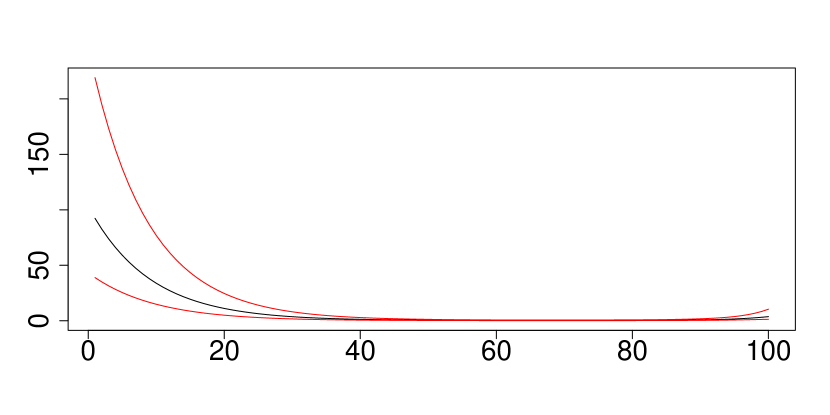
We first discuss the non-linear relationship between mortality rates and ISI. Figure 2 shows that GAMs predict similar smoothing patterns for the following mortality causes, endocrine, nutritional and metabolic diseases in Figure 2(5), psychic and behavioral disorders in Figure 2(6), diseases of the nervous system and sense organs in Figure 2(7), diseases of the circulatory system in Figure 2(8), diseases of the respiratory system in Figure 2(9), and external causes of trauma and poisoning in Figure 2(17). When the Italian government implemented loose intervention measures, the mortality rates went down as the intervention became more strict until intervention reached certain median-to-low level (ISI between 20 and 40), the mortality rates took a reverse trend and went up as more strict policies were carried out. In general, early and mild interventions like social distancing and improved hygiene practices not only reduced the spread of COVID-19 but also other infectious diseases, which could benefit individuals with a wide range of health conditions. The initial stages of the pandemic also led to increased health awareness and changes to more regular lifestyle. However, these benefits subsided as healthcare resources were increasingly diverted to treat COVID-19 patients, individuals with other health conditions might have faced delayed or reduced access to necessary health care. More specifically, for some individuals with psychic and behavioral disorders, when the intervention measures were mild, staying at home might have initially reduced stressors such as workplace pressures or social anxiety, potentially benefiting mental health, however, the potential benefits were replaced by increased isolation and loneliness, heightened anxiety and stress as well as substance abuse when situation deteriorated and higher lockdown levels were enforced. As for diseases of the circulatory system and diseases of the respiratory system, initial reduction of mortality rates at low ISI levels could also be attributed to factors like reduction in air pollution, reduced exposure to allergens, less physical strain from commuting as a result of early intervention procedures. Lastly, we comment on external causes of trauma and poisoning. In the early stages of the pandemic, there was rising public vigilance and a focus on safety, which might have extended beyond COVID-19 precautions to general safety practices, potentially reducing accidents. Meanwhile, people were adapting to new routines which might have included safer practices at home, reducing the risk of domestic accidents or poisonings. When the stringency measures prolonged, people started to be impacted by mental health issues as well as social and economic hardship, which could potentially contribute to the upward trend.

Refer to caption
(1) COVID-19
Refer to caption
(2) Some infectious and parasitic diseases
Refer to caption
(3) Tumors
Refer to caption
(4) Diseases of the blood and hematopoietic organs and some disorders of the immune system
Refer to caption
(5) Endocrine, nutritional and metabolic diseases
Refer to caption
(6) Psychic and behavioral disorders
Refer to caption
(7) Diseases of the nervous system and sense organs
Refer to caption
(8) Diseases of the circulatory system
Refer to caption
(9) Diseases of the respiratory system
Refer to caption
(10) Diseases of the digestive system
Refer to caption
(11) Diseases of the skin and subcutaneous tissue
Refer to caption
(12) Diseases of the musculoskeletal system and connective tissue
Refer to caption
(13) Diseases of the genitourinary system
Refer to caption
(14) Some morbid conditions that originate in the perinatal period
Refer to caption
(15) Congenital malformations and chromosomal anomalies
Refer to caption
(16) Symptoms, signs, abnormal results and ill-defined causes
Refer to caption
(17) External causes of trauma and poisoning
Figure 2: Estimated mortality rates of 17 causes as a function of Italian Stringency Index (ISI). Black lines are estimated values and red lines are 95% credible intervals.

Another common non-linear pattern of predicted mortality rates by ISI shared among some mortality causes is an overall downward trend. The mortality causes exhibiting such behaviors are some infectious and parasitic diseases in Figure 2(2), tumors in Figure 2(3), diseases of the digestive system in Figure 2(10), diseases of the skin and sub-cutaneous tissue in Figure 2(11) and congenital malformations and chromosomal anomalies in Figure 2(15). For these causes, benefits of social distancing due to high stringency levels dominates factors such as disrupted health care access, delayed diagnoses and treatments. We also note that credible intervals are wider when ISI is close to 100, suggesting distinct mortality patterns appearing in different regions and age groups.

We selected to display three representative mortality patterns between age and causes of death in Figure 3. Almost all mortality causes show the same feature that the mortality increases with age, similar to the pattern of some infectious and parasitic diseases shown in Figure 3(2). The mortality rate of COVID-19, however, peaked around slightly over 80 years old. Although there have been studies pointing out that age is a positive predictor of the morality rate (Bonanad et al.,, 2020; Zhang et al.,, 2023), their stratification usually sets 80 years old and above as a group. The age groups in the data set that we analyse are more refined with 4 separate age groups for age 80+. Our result offers new insights on the relationship between COVID-19 mortality and age.
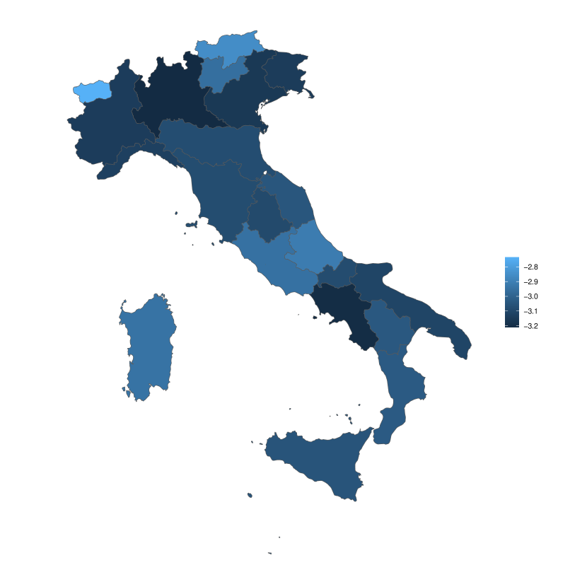
Refer to caption
(1) COVID-19
Refer to caption
(2) Some infectious and parasitic diseases
Refer to caption
(3) Some morbid conditions that originate in the perinatal period
Figure 3: Estimated mortality rates of 3 selected causes as a function of age. Black lines are estimated values and red lines are 95% credible intervals.

As for temporal evolving zn,tz_{n,t}^{*} in the Poisson rates, we focus on three aspects. The approximated posterior distribution of 𝝁\bm{\mu} indicates the average mortality levels of each cause of death in each region unexplained by covariates in the model. From Figure 5, we can see that both tumors in Figure 4(3) and diseases of the circulatory system in Figure 4(8) contribute most to death counts whereas some morbid conditions that originate in the perinatal period shown in Figure 5(5) have the lowest mortality rate on average. Figure 5 also reveals certain geographical disparity. For instance, Piedmont, Liguria, Apulia and Abruzzo are the regions mostly affected by COVID-19 according to Figure 4(1), however this conclusion is in contradiction with the observation that regions such as Lombardy, Veneto, and Campania experienced many cases and deaths. Recall that 𝝁\bm{\mu} measures unexplained mortality rate per 1,000 cases since we include COVID-19 cases in offset ϵn,t\epsilon_{n,t}, the discrepancy could be attributed to factors including healthcare system quality, timing of the outbreak, testing capacity and so on. For example, regions with less comprehensive testing may report fewer mild or asymptomatic cases, resulting in a higher mortality rate, as the total cases are underestimated. Nevertheless, to answer this question, we need access to more covariates. Certain regional gap is more in line with conventional knowledge. Figure 4(5) shows that endocrine, nutritional and metabolic diseases are more deadly in the south as southern regions have higher rates of obesity and diabetes. Temperature is another risk factor behind the phenomenon.

Refer to caption
(1) COVID-19
Refer to caption
(2) Some infectious and parasitic diseases
Refer to caption
(3) Tumors
Refer to caption
(4) Diseases of the blood and hematopoietic organs and some disorders of the immune system
Refer to caption
(5) Endocrine, nutritional and metabolic diseases
Refer to caption
(6) Psychic and behavioral disorders
Refer to caption
(7) Diseases of the nervous system and sense organs
Refer to caption
(8) Diseases of the circulatory system
Refer to caption
(9) Diseases of the respiratory system
Figure 4: Estimated mortality means 𝝁\bm{\mu} of 17 causes in 21 Italian regions.
Refer to caption
(1) Diseases of the digestive system
Refer to caption
(2) Diseases of the skin and subcutaneous tissue
Refer to caption
(3) Diseases of the musculoskeletal system and connective tissue
Refer to caption
(4) Diseases of the genitourinary system
Refer to caption
(5) Some morbid conditions that originate in the perinatal period
Refer to caption
(6) Congenital malformations and chromosomal anomalies
Refer to caption
(7) Symptoms, signs, abnormal results and ill-defined causes
Refer to caption
(8) External causes of trauma and poisoning
Figure 5: Estimated mortality means 𝝁\bm{\mu} of 17 causes in 21 Italian regions.

We now discuss the other two aspects associated with zn,tz^{*}_{n,t}, the dependence structure captured by (Vq,l)Vq,l(V^{q,l})^{\prime}V^{q,l} for the scale matrix Dq,lD^{q,l} of the variational Wishart density and the correlation captured by (Vq,k)Vq,k(V^{q,k})^{\prime}V^{q,k} for the scale matrix Dq,kD^{q,k}. Since Dq,lD^{q,l} contains spatial information that controls the dynamic of zn,tz^{*}_{n,t}, we compute the partial correlation matrix, that is the normalized inverse, of Dq,lD^{q,l} and then set the entries in the inverse matrix whose absolute value are below 0.1 to 0 while replace the remaining entries with 1. Figure 6(1) maps the resulting adjacency matrix into Italy where red edges between two regions stand for 1’s in the adjacency matrix, indicating a direct statistical relationship between them that is not explained by their relationships with other regions. There edges form four clusters; northern Italian regions are connected, and Lombardy appears to be the central hub for disease spread with many edges connected to it, possibly due to higher mobility or being a major transportation center. The remaining three clusters lie in the center and the southern Italy. The behavior indicates that regions inside each cluster might experience similar trends in mortality rates due to migration patterns, economic ties, climate conditions, or population behaviors. On the other hand, the absence of an edge between two regions implies conditional independence, meaning that once the influence of all other regions is controlled for, there is no direct statistical relationship between these two regions. This is the case with most regions.

Lastly, we turn to the correlation structure among various mortality causes. Figure 6(2) shows strong positive correlation inside the following 5 causes of death, endocrine, nutritional and metabolic diseases, psychic and behavioral disorders, diseases of the nervous system and sense organs, diseases of the circulatory system, and diseases of the respiratory system. In terms of the relationship between COVID-19 and other causes of death, we only observe weak negative relationship between COVID-19 and symptoms, signs, abnormal results and ill-defined causes, which suggests that improved detection of COVID-19 death likely reduced the number of deaths classified under ill-defined causes. The lack of correlation between between COVID-19 and other causes of death indicates that after controlling government intervention intensity during the pandemic, COVID-19 itself does not have strong influence on moralities in other death categories.

Refer to caption
(1) regional network from Dq,lD^{q,l}
Refer to caption
(2) correlation matrix from Dq,kD^{q,k}
Figure 6: Partial correlation and correlation derived from the optimal scale matrix of variational Wishart density.

5 Summary and Future Work

We develop an effiecient variational inference procedure for Bayesian dynamic GAMs where the dependent variable follows a Poisson distribution. The GAM component in the Poisson rate captures non-linear relationship between the outcome and covariates while the dynamics in the rate has a state space representation. The latent states in the model are assumed to be stationary with covariance matrix defined using a Kronecker product that disentangles one large covariance matrix into smaller covariance matrices. High-dimensional setting is considered, which prohibits the use of exact sampling algorithms, therefore we adopt variational algorithm to achieve fast convergence. The approach is applied to Italian mortality data to facilitate our understanding of mortality pattern changes during the COVID-19 outbreak.

Even though we concentrate on explanatory power of the model, it is potentially suitable for forecasting as the state space component models dynamics in mortality patterns. Another extension makes more sophisticated assumptions on the covariance matrix of the latent states. For instance, it is interesting to impose hierarchical G-Wishart distribution prior instead of Wishart prior on the precision matrices so that conditional dependence structure can be directly inferred from the model. Alternatively, the covariance matrix can be time-varying, allowing for more flexibility to account for changes in the dependence structure, especially before the COVID-19 pandemic and after the pandemic. We leave these discussion to future work.

References

  • Abedi et al., (2021) Abedi, V., Olulana, O., Avula, V., Chaudhary, D., Khan, A., Shahjouei, S., Li, J., and Zand, R. (2021). Racial, economic, and health inequality and COVID-19 infection in the united states. Journal of Racial and Ethnic Health Disparities, 8:732–742.
  • Anderson et al., (1958) Anderson, T. W., Anderson, T. W., Anderson, T. W., Anderson, T. W., and Mathématicien, E.-U. (1958). An introduction to multivariate statistical analysis, volume 2. Wiley New York.
  • Arridge et al., (2018) Arridge, S. R., Ito, K., Jin, B., and Zhang, C. (2018). Variational gaussian approximation for poisson data. Inverse Problems, 34(2):025005.
  • Basellini and Camarda, (2022) Basellini, U. and Camarda, C. G. (2022). Explaining regional differences in mortality during the first wave of COVID-19 in italy. Population Studies, 76(1):99–118.
  • Bertsekas, (1982) Bertsekas, D. P. (1982). Projected newton methods for optimization problems with simple constraints. SIAM Journal on Control and Optimization, 20(2):221–246.
  • Beskos et al., (2014) Beskos, A., Crisan, D., and Jasra, A. (2014). On the stability of sequential Monte Carlo methods in high dimensions. The Annals of Applied Probability, 24(4):1396 – 1445.
  • Blei et al., (2017) Blei, D. M., Kucukelbir, A., and McAuliffe, J. D. (2017). Variational inference: A review for statisticians. Journal of the American Statistical Association, 112(518):859–877.
  • Bonanad et al., (2020) Bonanad, C., García-Blas, S., Tarazona-Santabalbina, F., Sanchis, J., Bertomeu-González, V., Fácila, L., Ariza, A., Núñez, J., and Cordero, A. (2020). The effect of age on mortality in patients with COVID-19: a meta-analysis with 611,583 subjects. Journal of the American Medical Directors Association, 21(7):915–918.
  • Carpenter et al., (2017) Carpenter, B., Gelman, A., Hoffman, M. D., Lee, D., Goodrich, B., Betancourt, M., Brubaker, M. A., Guo, J., Li, P., and Riddell, A. (2017). Stan: A probabilistic programming language. Journal of Statistical Software, 76.
  • Clark and Wells, (2023) Clark, N. J. and Wells, K. (2023). Dynamic generalised additive models (dgams) for forecasting discrete ecological time series. Methods in Ecology and Evolution, 14(3):771–784.
  • Conteduca and Borin, (2022) Conteduca, F. P. and Borin, A. (2022). A new dataset for local and national COVID-19-related restrictions in italy. Italian Economic Journal, 8(2):435–470.
  • Dmetrichuk et al., (2022) Dmetrichuk, J. M., Rosenthal, J. S., Man, J., Cullip, M., and Wells, R. A. (2022). Retrospective study of non-natural manners of death in ontario: effects of the COVID-19 pandemic and related public health measures. The Lancet Regional Health-Americas, 7:100130.
  • Doucet et al., (2001) Doucet, A., De Freitas, N., Gordon, N. J., et al. (2001). Sequential Monte Carlo methods in practice, volume 1. Springer.
  • Durbin and Koopman, (2012) Durbin, J. and Koopman, S. J. (2012). Time series analysis by state space methods, volume 38. OUP Oxford.
  • Feng, (2022) Feng, C. (2022). Spatial-temporal generalized additive model for modeling COVID-19 mortality risk in toronto, canada. Spatial Statistics, 49:100526.
  • Hale et al., (2021) Hale, T., Angrist, N., Goldszmidt, R., Kira, B., Petherick, A., Phillips, T., Webster, S., Cameron-Blake, E., Hallas, L., Majumdar, S., et al. (2021). A global panel database of pandemic policies (Oxford Covid-19 government response tracker). Nature Human Behaviour, 5(4):529–538.
  • Hastie and Tibshirani, (1987) Hastie, T. and Tibshirani, R. (1987). Generalized additive models: some applications. Journal of the American Statistical Association, 82(398):371–386.
  • Hastie, (2017) Hastie, T. J. (2017). Generalized additive models. In Statistical models in S, pages 249–307. Routledge.
  • Jordan et al., (1999) Jordan, M. I., Ghahramani, Z., Jaakkola, T. S., and Saul, L. K. (1999). An introduction to variational methods for graphical models. Machine Learning, 37:183–233.
  • Koum Besson et al., (2021) Koum Besson, E. S., Norris, A., Bin Ghouth, A. S., Freemantle, T., Alhaffar, M., Vazquez, Y., Reeve, C., Curran, P. J., and Checchi, F. (2021). Excess mortality during the COVID-19 pandemic: a geospatial and statistical analysis in aden governorate, yemen. BMJ Global Health, 6(3):e004564–e004564.
  • Kretzschmar et al., (2020) Kretzschmar, M. E., Rozhnova, G., Bootsma, M. C., van Boven, M., van de Wijgert, J. H., and Bonten, M. J. (2020). Impact of delays on effectiveness of contact tracing strategies for COVID-19: a modelling study. The Lancet Public Health, 5(8):e452–e459.
  • Mitchell and Li, (2021) Mitchell, T. O. and Li, L. (2021). State-level data on suicide mortality during COVID-19 quarantine: early evidence of a disproportionate impact on racial minorities. Psychiatry Research, 295:113629.
  • Msemburi et al., (2023) Msemburi, W., Karlinsky, A., Knutson, V., Aleshin-Guendel, S., Chatterji, S., and Wakefield, J. (2023). The WHO estimates of excess mortality associated with the COVID-19 pandemic. Nature, 613(7942):130–137.
  • Nazia et al., (2022) Nazia, N., Law, J., and Butt, Z. A. (2022). Identifying spatiotemporal patterns of COVID-19 transmissions and the drivers of the patterns in toronto: a bayesian hierarchical spatiotemporal modelling. Scientific Reports, 12(1):9369.
  • Pell et al., (2020) Pell, R., Fryer, E., Manek, S., Winter, L., and Roberts, I. S. (2020). Coronial autopsies identify the indirect effects of COVID-19. The Lancet Public Health, 5(9):e474.
  • Peretti-Watel et al., (2020) Peretti-Watel, P., Seror, V., Cortaredona, S., Launay, O., Raude, J., Verger, P., Fressard, L., Beck, F., Legleye, S., l’Haridon, O., et al. (2020). A future vaccination campaign against COVID-19 at risk of vaccine hesitancy and politicisation. The Lancet Infectious Diseases, 20(7):769–770.
  • Petris et al., (2009) Petris, G., Petrone, S., and Campagnoli, P. (2009). Dynamic linear models with R. Springer Science & Business Media.
  • Plummer et al., (2003) Plummer, M. et al. (2003). Jags: A program for analysis of bayesian graphical models using gibbs sampling. In Proceedings of the 3rd international workshop on distributed statistical computing, volume 124, pages 1–10. Vienna, Austria.
  • Quiroz et al., (2023) Quiroz, M., Nott, D. J., and Kohn, R. (2023). Gaussian variational approximations for high-dimensional state space models. Bayesian Analysis, 18(3):989–1016.
  • Rao and Molina, (2015) Rao, J. N. and Molina, I. (2015). Small area estimation. John Wiley & Sons.
  • Shiels et al., (2022) Shiels, M. S., Haque, A. T., de González, A. B., and Freedman, N. D. (2022). Leading causes of death in the us during the COVID-19 pandemic, march 2020 to october 2021. JAMA Internal Medicine, 182(8):883–886.
  • Smith et al., (2015) Smith, T. R., Wakefield, J., and Dobra, A. (2015). Restricted covariance priors with applications in spatial statistics. Bayesian Analysis, 10(4):965.
  • Smith and Hocking, (1972) Smith, W. and Hocking, R. (1972). Algorithm as 53: Wishart variate generator. Journal of the Royal Statistical Society. Series C (Applied Statistics), 21(3):341–345.
  • Tan and Nott, (2018) Tan, L. S. and Nott, D. J. (2018). Gaussian variational approximation with sparse precision matrices. Statistics and Computing, 28:259–275.
  • Tibshirani, (2015) Tibshirani, R. J. (2015). A general framework for fast stagewise algorithms. Journal of Machine Learning Research, 16(1):2543–2588.
  • Titsias and Lázaro-Gredilla, (2014) Titsias, M. and Lázaro-Gredilla, M. (2014). Doubly stochastic variational bayes for non-conjugate inference. In International conference on machine learning, pages 1971–1979. PMLR.
  • Van Leeuwen et al., (2019) Van Leeuwen, P. J., Künsch, H. R., Nerger, L., Potthast, R., and Reich, S. (2019). Particle filters for high-dimensional geoscience applications: A review. Quarterly Journal of the Royal Meteorological Society, 145(723):2335–2365.
  • Walker and Ni, (2011) Walker, H. F. and Ni, P. (2011). Anderson acceleration for fixed-point iterations. SIAM Journal on Numerical Analysis, 49(4):1715–1735.
  • Wang et al., (2022) Wang, H., Paulson, K. R., Pease, S. A., Watson, S., Comfort, H., Zheng, P., Aravkin, A. Y., Bisignano, C., Barber, R. M., Alam, T., et al. (2022). Estimating excess mortality due to the COVID-19 pandemic: a systematic analysis of COVID-19-related mortality, 2020–21. The Lancet, 399(10334):1513–1536.
  • WHO, (1992) WHO (1992). The ICD-10 classification of mental and behavioural disorders: clinical descriptions and diagnostic guidelines, volume 1. World Health Organization.
  • Wood, (2017) Wood, S. N. (2017). Generalized additive models: an introduction with R. CRC press.
  • Yin et al., (2023) Yin, X., Aiken, J. M., Harris, R., and Bamber, J. L. (2023). Spatio-temporal spread of COVID-19 and its associations with socioeconomic, demographic and environmental factors in england: A bayesian hierarchical spatio-temporal model. arXiv preprint arXiv:2308.09404.
  • Zhang et al., (2023) Zhang, J.-j., Dong, X., Liu, G.-h., and Gao, Y.-d. (2023). Risk and protective factors for COVID-19 morbidity, severity, and mortality. Clinical Reviews in Allergy & Immunology, 64(1):90–107.
  • Zhu et al., (2021) Zhu, G., Zhu, Y., Wang, Z., Meng, W., Wang, X., Feng, J., Li, J., Xiao, Y., Shi, F., and Wang, S. (2021). The association between ambient temperature and mortality of the coronavirus disease 2019 (COVID-19) in Wuhan, China: a time-series analysis. BMC Public Health, 21:1–10.